1–11
Solar and planetary dynamos:
comparison and recent developments
Abstract
While obviously having a common root, solar and planetary dynamo theory have taken increasingly divergent routes in the last two or three decades, and there are probably few experts now who can claim to be equally versed in both. Characteristically, even in the fine and comprehensive book “The magnetic Universe” (Rüdiger & Hollerbach 2004), the chapters on planets and on the Sun were written by different authors. Separate reviews written on the two topics include Petrovay (2000), Charbonneau (2005), Choudhuri (2008) on the solar dynamo and Glatzmaier (2002), Stevenson (2003) on the planetary dynamo. In the following I will try to make a systematic comparison between solar and planetary dynamos, presenting analogies and differences, and highlighting some interesting recent results.
keywords:
magnetic fields, MHD, plasmas, turbulence, Sun: magnetic fields, Sun: interior, Earth, planets and satellites: general1 Approaches to astrophysical dynamos
1.1 Dimensional analysis: mixing-length vs. magnetostrophic balance
Faced with a problem like the dynamo, where the governing equations are well known and the source of difficulties is their complexity, it is advisable to start by order of magnitude estimates of the individual terms in the equations. A clear and detailed account of this is given in Starchenko & Jones (2002).
In the case of the Sun, such considerations point to a balance between buoyancy and inertial forces as the determinant of the resulting flow pattern in the convective zone. Indeed, the order of magnitude equality of these terms is one of the basic formulæ of the mixing length theory of astrophysical convection, as formulated in the 1950s —so this balance is customarily referred to as “mixing length balance” in the dynamo literature.
On the other hand, in rapidly rotating rotating systems the Coriolis term dominates over the inertial term. If the magnetic field is strong enough for Lorentz forces to be comparable to the Coriolis force and the buoyancy, another type of balance known as magnetostrophic balance (or MAC balance) sets in. This kind of balance is now generally thought to prevail in the more “mainstream” planetary dynamos, such as those of Earth, Jupiter, Saturn, and possibly Ganymede.
1.2 Implicit models: Mean field theory
As the smallest and largest structures present in the strongly turbulent astrophysical dynamos are separated by many orders of magnitude, it is hopeless and perhaps unnecessary to set the full explicit treatment of all scales of motion as a goal. In this sense, all models of astrophysical dynamos are necessarily “mean field models”, not resolving scales smaller than a certain level and representing the effect of those scales with some effective diffusivities. Yet the term “mean field theory” is customarily reserved for those models where even the largest scale turbulent motions, thought to be the main contributors to dynamo action, remain unresolved.
Mean field theory has remained the preferred theoretical tool of solar dynamo studies. Even the effect of obviously non-mean-field effects can be included in mean field models in the form of parametrized ad hoc terms. E.g. the emergence of strong magnetic flux loops from the tacholine to the photosphere is now thought by some to be a major contributor to the -effect (the so-called Babcock-Leighton mechanism for ). The motion of magnetized fluid being highly independent of the rest of the plasma, this may appear to be a case where the mean field description is bound to fail —but the problem is circumvented in mean field dynamo models e.g. by the introduction of a non-local -term (Wang et al. 1991) or by using different diffusivity values for poloidal and toroidal fields (Chatterjee et al. 2004).
1.3 Explicit models: Numerical simulations
In contrast to solar dynamo theory, planetary dynamo studies have traditionally focused on models where the large scale, rotationally influenced turbulent motions are explicitly resolved. For a long time such studies were essentially kinematical, prescribing the large scale flows by simple mathematical formulæ that satisfy some more or less well founded basic physical expectations, and solving only the induction equation. Such studies can still significantly contribute to our understanding of dynamos (see e.g. Gubbins 2008 for a recent overview). Yet, from the mid-1990s onwards the rapid increase in computer power has made it possible to develop explicit dynamical models (aka numerical simulations) of the geodynamo, and this has become the main trend in planetary dynamo research.
2 Observational constraints
We are separated from the Earth’s outer core by 3000 km of intransparent rock, while the top of Sun’s convective zone is directly observable across 1 AU of near-empty space. Although magnetic measurements and seismology in principle allow indirect inferences on conditions in the outer core, these are both limited to relatively large-scale (spherical harmonic degree ) magnetic structures, while empirical information on flows in the core is almost completely lacking.
In sharp contrast to this, the brightness of the Sun allows high S/N detection of spectral line profiles, permitting a precise determination of Doppler and Zeeman shifts. This not only provides a wealth of high-resolution observations of flows and magnetic fields at the top of the convective zone: the sensitive detection of waves and oscillations in the solar photosphere also allows a detailed reconstruction of flows and magnetic field patterns in layers lying below the surface.
The different amount of empirical constraints are certainly a major factor in determining the different approaches taken by solar and planetary dynamo studies. The main shortcoming of mean field models impeding progress is the vast number of possibilities available for the choice of parameters and their profiles, which renders the formulation of mean field dynamo models for the planets a rather idle enterprise. The good empirical constraints in the solar case provide an indispensable support by narrowing down the range of admissible models. It is no coincidence that it was the helioseismic determination of the internal rotation profile around 1990 which led to a resurgence in solar mean field dynamo theory.
At the same time, no MHD numerical simulation of the solar convective zone has been able to recover the observed butterfly diagram, and even reproducing the observed differential rotation profile is not trivial (cf. Sect. 6 below). Geodynamo simulations correctly reproduce nearly all the known spatiotemporal variance in the Earth’s magnetic field, and recently there are indications that they could provide a successful general scheme to understand the variety of dynamos seen in the Solar System (see Sect. 8).
3 State of matter, stratification
One obvious difference between planetary and stellar dynamos is that while the conducting matter in stars is ionised gas, in planetary dynamos it’s conducting liquids. The consequences of this are twofold. On the one hand, in planets incompressibility is often a good approximation, whereas in the Sun there many scale heights between the top and bottom of the SCZ and the scale height itself varies by several orders of magnitude. This extreme stratification or “stacking” of structures of vastly different scale is one major obstacle in the way of realistic global simulations of the SCZ.
Another consequence of the different state of matter in stellar and planetary dynamos is that molecular transport coefficients or diffusivities (such as viscosity, resistivity or heat diffusivity) are less accurately and reliably known in planetary interiors, given the more complex material structure. Together with the unsatisfactorily constrained thermal state, this means that the exact position, boundaries and even nature of the dynamo shell is in doubt in some planets. In the water giants (Uranus and Neptune) the resistivity of their electrolytic mantles is very uncertain, affecting the extent and depth of the dynamo layer. In Mercury, the unknown thermal state of the planet and the unknown amount of light constituents make the position and thickness of the liquid outer core rather uncertain. (Evidence for a liquid outer core was recently reported by Margot et al. 2007.)
4 Energetics and importance of chemistry
The energy source of the convective motions giving rise to the dynamo introduces further divisions into astrophysical dynamos. Jupiter, Saturn and the Sun are luminous enough to drive vigorous convection in their interiors by thermal effects alone. For terrestrial planets the available remanent heat may be only barely sufficient or even insufficient to maintain core convection. In these objects, chemical or compositional driving may be an important contribution to maintaining the convective state of their cores. (See e.g. Stevenson 2003 for numerical estimates.) In the case of the Earth, the most likely candidate is the piling up of light constituents like sulphur at the bottom of the outer core, as iron is freezing out onto the inner core and the light elements are locked out of the solid phase. (Arguments for an analoguous mechanism suggested for Saturn, the “helium rain” now seem to have been weakened by the new results of Stixrude & Jeanloz 2008.)
5 Boundaries and adjacent conducting flows
One important new contribution of numerical simulations was the realization of the crucial role that the choice of boundary conditions play in determining the solutions. Indications for this effect had already been found in kinematic dynamo calculations: e.g. the assumed conductivity of the solid inner core in a geodynamo model affects strongly its capability to maintain a dipole dominated field and the frequency of reversals (Hollerbach & Jones 1993). But the most important effect is due to the thermal boundary conditions. Convection is driven by heat input from below and heat loss from the top of the layer. In terrestrial planets the latter occurs by mantle convection, the efficiency of which is then a fundamental determinant of the behaviour of the dynamo. Indeed, as the timescale of mantle flows is very long compared to those in the dynamo, in addition to the overall mantle convection even the instantaneous convection pattern realized now can have a profound effect on the flow structure in the geodynamo (Glatzmaier 2002). The most widely mentioned possibility why Venus does not seem to support a dynamo is that, lacking plate tectonics, Venus’ mantle convection is less efficient, so its heat flux can be transported conductively throughout the core, and no convective instability arises. The resulting slower cooling of the planet may have the additional result that no inner core has solidified yet, depriving Venus even of the alternative energy source for convection that an inverse molecular weight gradient could provide (Stevenson 2003).
The importance of appropriate boundary conditions is now also recognized in simulations of the solar convective zone. Despite repeated attempts with ever more powerful computers, the hydrodynamical simulations of the new millennium had until very recently not been able to reproduce the observed solar internal rotation profile, the resulting isorotation surfaces being cylindrical rather than conical (e.g. Brun & Toomre 2002). The most recent state-of-the-art simulation (Miesch et al. 2008), however, brought a breakthrough in this respect. The breakthrough is not due to the higher computing power available, but to the introduction of a small (%) pole-equator temperature difference at the bottom boundary. While at first sight ad hoc, the introduction of this difference had the beneficial effect of leading to a realistic differential rotation and a realistic meridional circulation at the same time, raising hopes that this may indeed be the right way out of the dilemma. This is so despite the fact that this solution of the problem may strike one as “æsthetically” less attractive, as the conical isorotation surfaces are attributed to a chance cancellation of two opposing effects, rather than to some deeper physical motive.
A further important factor that may fundamentally affect the behaviour of a dynamo is the presence or absence of conducting stable fluid layers in its vicinity. Such a layer, the solar tachocline, is certainly present below the solar convective zone, and is currently thought to play a major role in the global solar dynamo (Forgács-Dajka & Petrovay 2002; Forgács-Dajka 2003). The strong stratification of the solar convective zone discussed above, has long been expected to give rise to pronounced transport effects or “pumping” mechanisms (see Petrovay 1994 for a comprehensive treatment of these effects). These pumping processes can efficiently remove most of the large-scale magnetic flux from the turbulent region, provided there is an adjacent region with high but finite conductivity that can receive and store this flux. Following earlier simpler numerical experiments, recent MHD numerical simulations have indeed shown the pumping of large scale magnetic flux from the convective zone into the tachocline below, where it forms strong coherent toroidal fields (Browning et al. 2006).
Similar conductive layers adjacent to the turbulent dynamo region may be present in some planetary interiors. Even in the case Earth it has been hypothesized that, as a result of convection, lighter elements ultimately pile up below the the CMB, resulting in a stably stratified sublayer within the outer core (Whaler 1980). The effect of such layers on the dynamo has not been studied extensively, but available results indicate that their impact on the observed field may be very important (Schubert et al. 2004).
6 Regime of operation
6.1 Dimensional and nondimensional parameters
The number of parameters uniquely determining a dynamo is quite limited. The geometry is a spherical shell between radii and , with thickness and relative thickness parameter . The shell, rotating with angular velocity , is filled with material of density , characterized by momentum, heat and magnetic diffusivities , and , respectively. Finally, convection in the shell is driven by the buoyancy flux fed in at the bottom of the shell (Olson & Christensen 2006). An internal heating may be added to the list for cases where volumetric heat loss from secular cooling or radioactive decay is significant.
The number of relevant parameters can be reduced further, realizing that the role of some of the variables is just to set characteristic scales. The length scale is clearly set by and the mass cale by . For the timescale it has been traditional for certain theoretical considerations to use the resistive time in dynamo theory. However, it was recently pointed out by Christensen & Aubert (2006) that for rapid rotators offers a more relevant scaling. Nondimensionalizing all parameters by these scales (and ignoring ) we are left with only 4 nondimensional parameters. Following Olson & Christensen (2006) the effective buoyant Rayleigh number can be defined as . The nondimensional measures of the diffusivities are the Ekman numbers
| (1) |
Instead of the three Ekman numbers, one Ekman number and two Prandtl numbers (i.e. diffusivity ratios) are more commonly used:
| (2) |
The specified parameters then, in principle, determine the solution, i.e. the resulting turbulent flow field and magnetic field. These can be characterized by their respective amplitudes and , as well as their typical length scale —say correlation length, integral scale or similar. (For simplicity a single length scale is assumed for both variables, ignoring anisotropy). In fact, these fiducial scales of the solution may even be estimated on dimensional grounds without actually solving the dynamo equations (Starchenko & Jones 2002). From and , turbulent diffusion coefficients can be estimated using the usual Austausch recipe . For the Sun, Earth and gas giants such estimates, summarized in Table 1, are in rough agreement with both observations and simulation results.
As nondimensional measures of and we introduce the Rossby and Lorentz numbers:
| (3) |
where is the Alfvén speed. It arguably makes more sense to use instead of in the above definitions, which leads us to “local” versions of these numbers:
| (4) |
Were we to adopt the diffusive time scales and instead of , the nondimensional measures of and would be the kinetic and magnetic Reynolds numbers:
| (5) |
(Again, using a “local” length parameter instead of may be more relevant.)
| Dynamo | [m/s] | [km] | [m2/s] |
|---|---|---|---|
| Sun (deep SCZ): | |||
| Earth: | 20 | ||
| Jupiter | – |
Let us now consider what the characteristic values of these nondimensional parameters are for astrophysical dynamos and for numerical simulations.
6.2 Ekman numbers (i.e. diffusivities)
Ekman numbers are extremely small in astrophysical dynamos, far below the range – accessible to current numerical simulations. The main obstacle to the further reduction of is that by choosing a realistic Rayleigh number, we fix the input of kinetic and magnetic energy into the system. In a stationary state energy must be dissipated at the same rate as it is fed in. The viscous dissipation rate is where is the smallest resolved scale —so cannot be reduced without also increasing the spatial resolution. The situation is similar for resistive (Ohmic) dissipation.
6.3 Reynolds numbers
It is interesting to note that the magnetic Reynolds number is the only parameter involving a diffusivity whose actual value can be used in current numerical simulations for some planets (including the Earth). Rossby numbers, in contrast, are invariably intractably small in planetary dynamos. The situation in the Sun is the reverse: Rossby numbers are moderate (only slightly below unity in the deep convective zone and actually quite high in shallow layers). Reynolds numbers, however, are all exteremely high in the solar plasma, even in the relatively cool photosphere.
The significance of consists in the existence of a critical value below which no dynamo action is possible. Planetary dynamo simulations have led to the surprising result that has a universal value of about 40, independently of the other parameters, specifically of the Prandtl numbers (Christensen & Aubert 2006). This is a surprising result as the expectation in turbulence theory, confirmed in numerical simulations of small-scale dynamos, has been that should be a sensitive function of (Boldyrev & Cattaneo 2004). The solution of this apparent contradiction is not known.
Elementary estimates show that the convective velocity resulting even for very slightly supercritical Rayleigh numbers results in magnetic Reynolds numbers well above . This implies that the conditions for convection and for dynamo action may be virtually identical in astrophysical fluid bodies with a high conductivity (Stevenson 2003). We have already seen that the apparent lack of dynamo action in Venus is attributed to the lack of convection in its core. Planets with very poorly conductive fluid layers, however, may obviously be convecting without supporting a dynamo. A case in point may be the water giants where the dynamo sustaining layer may potentially only extend to a thin sublayer of the convecting water mantle and/or be only slightly supercritical, unable to generate fields strong enough to reach magnetostrophic equilibrium.
6.4 Rossby number (i.e. velocity amplitude)
An important issue is how the Rossby and Lorentz numbers (i.e. nondimensional velocity and magnetic field amplitudes) scale with the input parameters of the dynamo problem. The significance of this is twofold. Firstly, as current numerical simulations cannot directly access the parameter range relevant for astrophysical dynamos, such scaling laws can be used to extrapolate their results into the physically interesting domain. Secondly, it is of interest to compare the scaling laws derived from simulation results to those predicted by physical considerations based on the concept of magnetostrophic equilibrium.
For the Rossby number, the scaling law extracted from simulations vs. the law theoretically expected for MAG balance are:
| (6) |
Geometrical factors invoked to explain the slight discrepancy in the values of the exponents do not seem to be capable of explaining it (Christensen & Aubert 2006). However, given the above mentioned doubt that the high values of the diffusivities employed may cast on all simulation results, one may also take the point of view that these two laws are actually in fairly good agreement, and no further explanation is needed. (Note that in this case the theoretical value 0.5 must be deemed the more reliable one.)
6.5 Lorentz number (i.e. magnetic field strength)
The scaling of the Lorentz number extracted from dipole-dominated dynamo simulations with no internal heating (Olson & Christensen 2006) viz. the MAC scaling following from the assumption of unit Elsässer number (Starchenko & Jones 2002) are
| (7) |
Assuming that the local Rossby number scales similarly to (6), the latter relation may also be turned into a scaling with , but its exponent (–) is even more discrepant from the value yielded by the simulations than in the previous case.
7 Predictive value
In solar dynamo theory there is a widely held belief that predictions for at least the next activity cycle should be possible. Dozens of methods have been proposed for this. The relatively most successful ones are apparently those based on some measure of solar activity or magnetism at the onset of the new cycle.Recently Cameron & Schüssler (2007) convincingly argued that what stands in the background of all such methods is just the well known Waldmeier effect, relating a cycle’s amplitude to the rate of rise of activity towards the maximum. As solar cycles are known to overlap by – years, the faster rise preceding a stronger cycle will result in an earlier epoch for the minimum —so it is natural to expect that at this time, polar magnetic fields and activity indices have not yet decayed to such low values as they reach during minima preceding weak cycles. Indeed, Cameron & Schüssler (2007) demonstrate that a very simple predictor, the value of the sunspot number three years before the minimum performs embarrassingly well (correlation coefficient 0.95) when it comes to predicting the amplitude of the next maximum, but this good performance is fully explained by the effect described above.
This is not to say that it would be pointless to rely on dynamo models to find a physical basis for activity predictions. Firstly, the Waldmeier effect itself is certainly due to some, as yet unclear, aspect of the dynamo. Second, there are grounds to assume that, at least in certain types of dynamos, there really is a physical relationship between high-latitude magnetic fields during the minimum and the amplitude of the next maximum (Choudhuri et al. 2007). Either way, the persistently low activity during the present solar minimum seems to be a strong indication that cycle 24 will be a rather weak one, in contrast to widely publicized claims based on a certain class of solar dynamo models (Dikpati & Gilman 2006).
Owing to the much longer timescales of planetary dynamos, the possibility for testable temporal predictions is limited. Planetary dynamo models can partly make up for this by the availability of several instances of known planetary dynamos. These inlcude 7 active dynamos (Mercury, Earth, Ganymede and the four giant planets) and one extinct dynamo (Mars), with the remaining planets also providing some important constraints precisely by apparently not supporting a dynamo. A testbed of a certain type of modelling approach, then, may be whether it is capable to provide a unified explanatory scheme for all these systems. Recent results suggest that planetary dynamo simulations may indeed provide such an explanatory scheme.
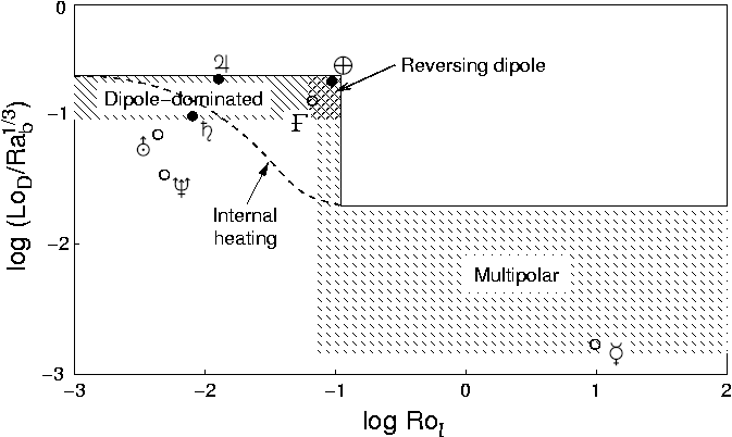
Collecting and homogenizing the results of hundreds of geodynamo simulations, Olson & Christensen (2006) find an interesting scaling (or rather, “non-scaling”) behaviour of the amplitude of the dipolar component of the resulting magnetic field. As mentioned above, considering only dipole-dominated dynamos without internal heating the scaling relationship (7) results for the amplitude of the dipole component. This scaling, however, is not valid for all dynamo models. This is borne out in Figure 1 where the ordinate essentially shows the ratio of the two sides of equation (7). The dipole-dominated cases in this plot will clearly lie along a horizontal line drawn at the ordinate value 0.5, corresponding to the coefficient in equation (7). This is indeed the case for dynamos where the Rossby number is low, i.e. where the driving is relatively weak. However, for Rossby numbers above a critical value of order 0.1, the amplitude of the dipolar component suddenly drops and the solution becomes multipolar. In the case of internally heated models the situation is similar, but the transition between the two regimes is more gradual.
The critical role of the Rossby number in this respect indicates that the underlying cause of the eventual collapse of the dynamo field is the increasing importance of inertial forces in the equation of motion (measured by the Rossby number). This leads to a breakup of the relatively regular columnar structures dominating rapidly rotating convection —the detailed mechanism of this will be discussed further in the next section.
A further interesting finding is that dynamos lying near the top of the Rossby number range of dipolar solutions are generally dipole-dominated, but occasionally undergo excursions and reversals. In a turbulent system this type of behaviour is rather plausible, given that parameters like are expected to fluctuate, and such fluctuations may occasionally take the system into multipolar regime, causing the dipolar field to collapse, and then reform once fluctuations have taken the system back to the dipolar regime.
Olson & Christensen (2006) also attempt to place individual planetary dynamos on the phase plane of Fig. 1, based on known empirical constraints and theoretical considerations. The resulting distribution seems to provide an impressively comprehensive classification system for planetary dynamos. Gas giants lie safely in the dipole-dominated regime, suggesting that their dynamos are in a magnetostrophic state maintaining a nonreversing dipolar field. Earth is found near the limit of the dipole-dominated regime, just where a dipolar dynamo known to be subject to occasional reversals is expected to be. A somewhat surprising conclusion of this scheme is that the planetary dynamo most similar to Earth’s in its behaviour may be Ganymede’s, also expected to maintain a reversing dipole. The fact the dipolar magnetic field amplitude of the water giants is significantly less than relations (7) predict, either be due to a significant amount of internal heating or to the low resistivity in their interiors, which prevents them from reaching magnetostrophic equilibrium. Finally, Fig. 1 would seems to suggest that, despite contrary opinions, Mercury should be expected to sustain a multipolar magnetic field structure.
Some caveats regarding Fig. 1 are in order. All the simulations upon which the figure is based were run with a shell thickness parameter , appropriate for the geodynamo. For planets with significantly different shell geometries, especially for those with thin shells (Mercury?; the water giants?), results may prove to be significantly different.
Note also that the parameter on the abscissa of Fig. 1 is actually a rather particular kind of Rossby number, involving one particular local turbulence timescale, defined in a way similar to the the Taylor microscale. As in current numerical simulations the largest and smallest scales are normally separated by no more than one order of magnitude, this fine distinction between different turbulent scales is not important. But when it comes to application to actual planets, the different turbulent timescales differ by many orders of magnitude, so choosing the right scale is critical. Christensen & Aubert (2006) provide good arguments for the choice of the particular form of used in Fig. 1, but it is still somewhat disconcerting that combining large-scale turbulent velocities with a much smaller length scale, the Rossby number loses its widely used physical interpretation as the ratio of rotational and turbulent turnover timescales. In addition, our limited knowledge on the spectrum of magnetostrophic turbulence (Zhang & Schubert 2000, Nataf & Gagnière 2008) makes it hard to derive a reliable value for the Taylor microscale in planetary dynamos: the Kolmogorov spectrum is just a (not too educated) guess.
8 Characteristic flow and field patterns
It is well known that solar activity phenomena appear collectively, in the form active regions. These regions are the solar atmospheric manifestations of large azimuthally oriented magnetic flux loops emerging through the convective zone. Indeed, the development of extremely successful detailed models of this emergence process, first in the thin fluxtube approximation, then in 3D numerical simulations, was probably the most spectacular success story of solar dynamo theory in the last few decades.
In contrast to our familiarity with the basic magnetic structures determining solar activity, nothing about analoguous structures in planetary dynamos had been known until very recently. This situation has spectacularly changed with the development of new visualization and geometrical analysis techniques, which showed that, just like in the Sun, the magnetic field in planetary dynamos is highly intermittent (25 % of the magnetic energy residing in just 1.6 % of the volume), and led to the recognition of a variety of field and flow structures (Aubert et al. 2008). The two main classes of such structures are magnetic cyclones/anticyclones and magnetic upwellings.
Magnetic cyclones and anticyclones are the MHD equivalent of Busse’s columnar structures, known to dominate rapidly rotating hydrodynamic convection. The simulations indicate that magnetic anticyclones, in particular, play a key role in generating and maintaining a dipole dominated magnetic field in the upper part of the dynamo layer and above. Near the bottom of the shell the field is invariably multipolar, but the thermal wind-driven upflow in the axis of a magnetic anticyclone amplifies the upward convected fields by stretching, so that at the top of the shell a predominantly dipolar field results.
Magnetic upwellings are buoyancy-driven upflows rising nearly radially through the shell owing to their high velocity. They come in two varieties: polar upwellings, limited to the interior of the tangent cylinder of the inner core, emerge more or less in parallel with the cyclonic/anticyclonic structures, while equatorial upwellings cut through those structures, disrupting their integrity. As a result, equatorial upwellings (distant cousines of the emerging magnetic flux loops in the Sun) are capable of interfering with the maintenance of an organized dipolar field by the magnetic anticyclones. As the buoyant driving, and in consequence the turbulent velocity (i.e. the Rossby number) is increased, the number and vigour of upwellings increases, until they can occasionally disrupt the dipolar magnetic field maintained by the magnetic anticyclones. Following such interruptions the dipole may be reformed with a polarity parallel or opposite to its previous polarity: such events correspond to magnetic excursions and reversals, respectively. Finally, with the further increase of the equatorial magnetic upflows permanently discapacitate the anticyclones, and the dominant dipolar field structure collapses. This is the mechanism in the background of the characteristic -dependence of dynamo configurations shown in Fig. 1 and discussed in the previous section. Thus, dynamo studies now seem to have elucidated, at least on a qualitative level, the basic mechanisms underlying the most characteristic phenomena of both solar and planetary dynamos.
Support by the Hungarian Science Research Fund (OTKA) under grant no. K67746 and by the EC SOLAIRE Network (MTRN-CT-2006-035484) is gratefully acknowledged.
References
- Aubert et al. (2008) Aubert, J., Aurnou, J., Wicht, J. 2008, Geophys. J. Intern. 172, 945
- Boldyrev & Cattaneo (2004) Boldyrev, S., Cattaneo, F. 2004, Phys. Rev. Lett. 92(14), 144501
- Browning et al. (2006) Browning, M. K., Miesch, M. S., Brun, A. S., Toomre, J. 2006, ApJ648, L157
- Brun & Toomre (2002) Brun, A. S., Toomre, J. 2002, ApJ570, 865
- Cameron & Schüssler (2007) Cameron, R., Schüssler, M. 2007, ApJ659, 801
- Charbonneau (2005) Charbonneau, P. 2005, Living Rev. Sol. Phys. 2, 2
- Chatterjee et al. (2004) Chatterjee, P., Nandy, D., Choudhuri, A. R. 2004, A&A427, 1019
- Choudhuri (2008) Choudhuri, A. R. 2008, Adv. Space Res. 41, 868
- Choudhuri et al. (2007) Choudhuri, A. R., Chatterjee, P., Jiang, J. 2007, Phys. Rev. Lett. 98(13), 131103
- Christensen & Aubert (2006) Christensen, U. R., Aubert, J. 2006, Geophys. J. Intern. 166, 97
- Dikpati & Gilman (2006) Dikpati, M., Gilman, P. A. 2006, ApJ649, 498
- Forgács-Dajka (2003) Forgács-Dajka, E. 2003, A&A413, 1143
- Forgács-Dajka & Petrovay (2002) Forgács-Dajka, E., Petrovay, K. 2002 A&A389, 629
- Glatzmaier (2002) Glatzmaier, G. 2002, Ann. Rev. Earth Pl. Sci. 30, 237
- Gubbins (2008) Gubbins, D. 2008, Geophys. J. Intern. 173, 79
- Hollerbach & Jones (1993) Hollerbach, R., Jones, C. A. 1993, Nature365, 541
- Margot et al. (2007) Margot, J. L., Peale, S. J., Jurgens, R. F., Slade, M. A., Holin, I. V. 2007, Science 316, 710
- Miesch et al. (2008) Miesch, M. S., Brun, A. S., DeRosa, M. L., Toomre, J. 2008, ApJ673, 557
- Nataf & Gagnière (2008) Nataf, H.-C., Gagnière, N. 2008, ArXiv e-prints, 805
- Olson & Christensen (2006) Olson, P., Christensen, U. R. 2006, Earth Plan. Sci. Lett. 250, 561
- Petrovay (1994) Petrovay, K. 1994, in R. J. Rutten, C. J. Schrijver (eds.), Solar Surface Magnetism, NATO ASI Series C433, Kluwer, Dordrecht, p. 415
- Petrovay (2000) Petrovay, K. 2000, in The Solar Cycle and Terrestrial Climate, ESA Publ. SP-463, p. 3
- Rüdiger & Hollerbach (2004) Rüdiger, G., Hollerbach, R. 2004, The Magnetic Universe, Wiley-VCH, Weinheim
- Schubert et al. (2004) Schubert, G., Chan, K. H., Liao, X., Zhang, K. 2004, Icarus 172, 305
- Starchenko & Jones (2002) Starchenko, S. V., Jones, C. A. 2002, Icarus 157, 426
- Stevenson (2003) Stevenson, D. J. 2003, Earth Pl. Sci. Lett. 208, 1
- Stixrude & Jeanloz (2008) Stixrude, L., Jeanloz, R. 2008, Proc. Natl. Acad. Sci. USA 105, 11071
- Wang et al. (1991) Wang, Y.-M., Sheeley, N. R., Nash, A. G. 1991, ApJ383, 431
- Whaler (1980) Whaler, K. A. 1980, Nature287, 528
- Zhang & Schubert (2000) Zhang, K., Schubert 2000, Ann. Rev. Earth Pl. Sci. 32, 409