Solving a Delay Differential Equation through Fourier Transform
Abstract
In this study, we introduce and explore a delay differential equation that lends itself to explicit solutions in the Fourier-transformed space. Through the careful alignment of the initial function, we can construct a highly accurate solution to the equation. These findings open new avenues for understanding delay systems, demonstrating the efficacy of Fourier transform techniques in capturing transient oscillatory dynamics.
Keywords: Delay, Transient Oscillation, Fourier Transform
1 Introduction
In various fields such as biology, mathematics, economics, and engineering, understanding the effects of delays has become an important issue [1, 2, 3, 4, 5, 6, 7, 8, 9, 10, 11, 12, 13, 14]. Even for simple systems, delays in feedback and/or interactions can induce oscillations and complex behaviors.“Delay Differential Equations” (DDEs) are crucial tools in such research. A representative example is the Mackey–Glass equation [8], which exhibits various types of dynamics, including chaos. Although our understanding of delay systems and DDEs has gradually improved (e.g.[15]), solving DDEs to obtain solutions is considered very difficult.
Typically, the problem of solving delay differential equations is to find a solution for , given the initial function for . We generally cannot obtain such solutions explicitly. Thus, the main analysis of the DDEs focuses on asymptotic stabilities and behaviors. Also, a recent analytical approach to simple DDEs uses the Lambert W function [16], which enables the expression of both formal and approximate solutions of the equation [17, 18, 19].
In this paper, we take an indirect path to obtain the solution of a DDE through the Fourier transform. Specifically, we examine our recently proposed DDE that has a linear time-dependent coefficient [20, 21]. With this DDE, the power spectrum peak of the dynamical trajectory reaches its maximum height when the delay is suitably tuned, indicating frequency resonance. Our focus here, however, is to show that we can solve this DDE explicitly in the Fourier-transformed space. We then numerically take the inverse Fourier transform to construct the solution for . The particular solution for , then, can be obtained if we view this solution by identifying the initial function with the above semi-numerically constructed function over . This provides a new approach to solve DDEs, and our DDE is a rare example where the solutions are obtained with high accuracy.
2 Delay Differential Equation
We proposed and studied the following delay differential equation [20, 21]:
| (1) |
where , , are real parameters, with interpreted as the delay.
This equation falls into a class of equations called non-autonomous DDEs, which have been studied in a more general context. Here, again, solving non-autonomous DDEs poses mathematical challenges[22, 23, 24, 25]. Additionally, we can view equation (1) as a slight modification of the well-studied Hayes equation, with only the second term replaced by a linear function of time rather than a constant. However, its behavior is quite distinct from that of the Hayes equation.
We have shown that for equation (1), oscillatory transient dynamics appear and disappear as the delay increases while maintaining asymptotic stability at . Also, frequency resonance is observed with the power spectrum peak of the dynamical trajectory reaching its maximum height when the delay is suitably tuned.
We list some properties of the special cases of equation (1):
-
•
With the delay and the initial condition , the solution to the equation is as follows:
(2) Thus, this solution exhibits a Gaussian shape with its peak at . Furthermore, with , we also note that equation (1) represents the annihilation operator equation of the quantum simple harmonic oscillator, with interpreted as a position rather than time (e.g.[26]). It has the Gaussian ground state as its solution.
-
•
The case where is a special case of the Hayes equation. In this case, the origin is asymptotically stable only within the range of
(3) However, with with a finite initial function, the asymptotic stability of the origin is kept for all delays. For the finite delays, the solution of equation (1) typically shows oscillatory dynamics.
For the finite delays, the solution of equation (1) typically shows oscillatory dynamics.
2.1 Solution through the Fourier Transform
Let us now explore finding a solution for equation (1) in the entire range of without specifying boundary conditions. We reasonably assume that with , the solution converges to for for finite solutions. Fourier transforming equation (1) yields:
| (4) |
where
| (5) |
Equation (4) can be easily solved, and the solution is given by:
| (6) |
where is an integration constant. Thus, we can assert the following:
The finite solution of equation (1) with in the range can be explicitly solved, and the solution is given by (6) in the Fourier-transformed space. This solution is unique up to the scale factor .
This leads to the following:
The finite solution of equation (1) with in the range can be obtained as follows through the inverse Fourier transform:
| (7) |
Again, the solution is unique up to the scale factor .
We observe that in the special case of , the inverse transform simplifies to the scenario of Gaussian integration. Consequently, we can explicitly express the limit as approaches infinity:
| (8) |
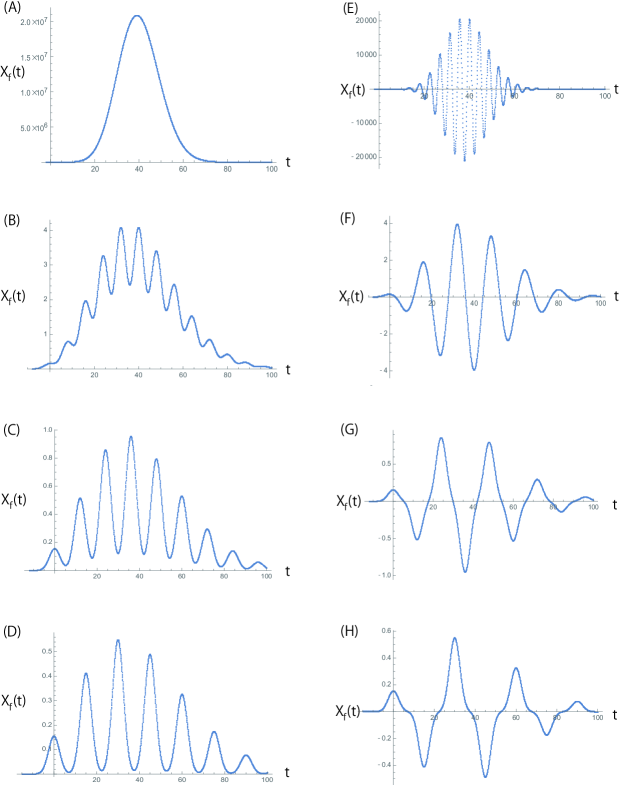
However, for the general case of , analytical integration of (7) is not feasible. Therefore, we resort to numerical integration, and representative results are depicted in Fig. 1.
3 Comparison with Numerical Solutions
Returning to equation (1) with , we seek a real solution in the range given the initial function , . Equation (1) with a general initial function remains unsolvable. However, the earlier findings suggest the following conjecture:
If the initial function is represented by the solution derived in equation (7) for , then the solution of equation (1) is expressed by for .
In other words, if a specific initial function is carefully selected such that it is the same as for , then the solution for is accurately given by for .
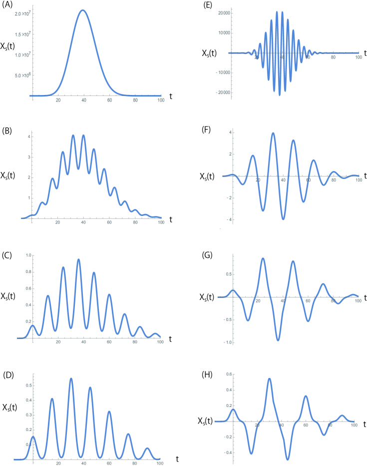
To verify the effectiveness of the proposed method for constructing a specific solution through the Fourier transform, we conducted direct numerical integration of equation (1). The initial condition was approximated by a 10th-order polynomial function: , chosen to closely match for . The corresponding results, aligned with those in Fig. 1, are illustrated in Fig. 2. For comparison, we also show Fig. 3, where the plots of Figs. 1 and 2 are overlaid.
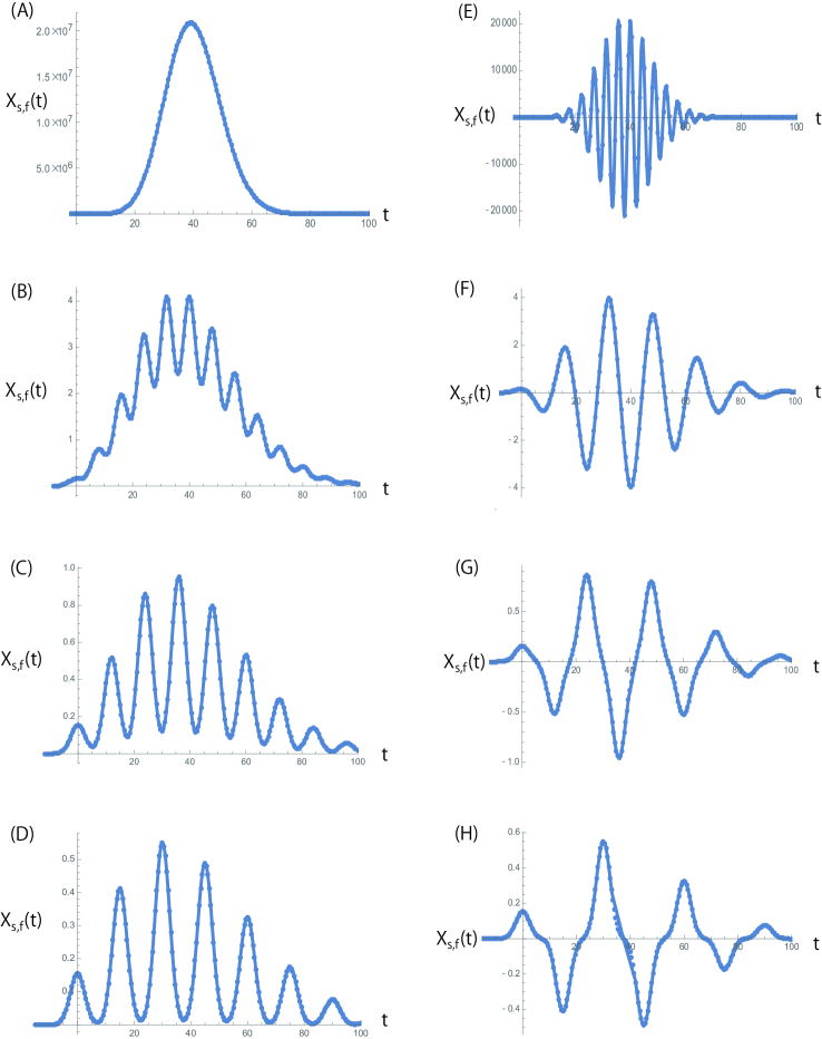
Our observation indicates that the semi-numerical construction of the solution for equation (1) through the Fourier transform can effectively capture the transient dynamics. This lends support to the reliability of our proposed approach.
4 Discussion
Several points warrant discussion regarding the findings presented.
1. Uncommon Capture of Transient Dynamics: It is noteworthy that capturing transient or non-equilibrium dynamical trajectories is often challenging, not only in the context of delay differential equations but also in general nonlinear dynamical systems(e.g. [27, 28]. Despite being semi-numerical, having concrete “solvable” examples, as demonstrated in this study, can contribute to a deeper understanding of non-linear transient phenomena.
2. Analytical Techniques and Challenges: In the analysis of delay differential equations, the predominant tool is often the use of the Laplace transform or equivalent techniques. These approaches are valuable for revealing stability characteristics of solutions. However, in the case of equation (1), the use of the Laplace transform does not yield an explicit solution, as achieved through the Fourier transform. The potential of further developing the Fourier transform approach to gain insight into the transient dynamics of general delay differential equations remains an open area for exploration.
3. Quantum Mechanical Connections: Another intriguing observation is that equation (1) with represents the annihilation operator equation for Quantum harmonic oscillators. Further differentiation of (1) with respect to time yields a second-order delay differential equation. Exploring this direction and potential connections to Quantum mechanics is left for future investigations.
In conclusion, the findings presented in this study offer a potential pathway to advancing our comprehension of delay differential equations. The application of Fourier transform techniques demonstrates promise in capturing transient non-linear dynamics. Also, the identified connections to Quantum mechanics present an intriguing direction for future research and exploration.
Acknowledgments
The authors would like to thank Prof. Hideki Ohira and the members of his research group at Nagoya University for their useful discussions. This work was supported by the “Yocho-gaku” Project sponsored by Toyota Motor Corporation, JSPS Topic-Setting Program to Advance Cutting-Edge Humanities and Social Sciences Research Grant Number JPJS00122674991, JSPS KAKENHI Grant Number 19H01201, and the Research Institute for Mathematical Sciences, an International Joint Usage/Research Center located at Kyoto University.
References
- [1] U. an der Heiden. “Delays in physiological systems,” J. Math. Biol., 8, 345–364 (1979).
- [2] R. Bellman and K. Cooke, Differential-Difference Equations (Academic Press, New York, 1963).
- [3] J. L. Cabrera and J. G. Milton, “On–off intermittency in a human balancing task,” Phys. Rev. Lett., 89, 158702 (2002).
- [4] N. D. Hayes, “Roots of the transcendental equation associated with a certain difference–differential equation,” J. Lond. Math. Soc., 25, 226–232 (1950).
- [5] T. Insperger, “Act-and-wait concept for continuous-time control systems with feedback delay,” IEEE Trans. Control Sys. Technol., 14, 974–977 (2007).
- [6] U. Küchler and B. Mensch, “Langevin’s stochastic differential equation extended by a time-delayed term,” Stoch. Stoch. Rep., 40, 23–42 (1992).
- [7] A. Longtin and J. G. Milton, “Insight into the transfer function, gain and oscillation onset for the pupil light reflex using delay-differential equations,” Biol. Cybern., 61, 51–58 (1989).
- [8] M. C. Mackey and L. Glass, “Oscillation and chaos in physiological control systems,” Science, 197, 287–289 (1977).
- [9] J Mitlon, J. L. Cabrera, T. Ohira, S. Tajima, Y. Tonosaki, C. W. Eurich, and S. A. Campbell, “The time–delayed inverted pendulum: Implications for human balance control,” Chaos, 19, 026110 (2009).
- [10] T. Ohira and T. Yamane. “Delayed stochastic systems,” Phys. Rev. E, 61, 1247–1257 (2000).
- [11] H. Smith, An introduction to delay differential equations with applications to the life sciences (Springer, New York, 2010).
- [12] G. Stépán, Retarded dynamical systems: Stability and characteristic functions ( Wiley & Sons, New York, 1989).
- [13] G. Stépán and T. Insperger, “Stability of time-periodic and delayed systems: a route to act-and-wait control,” Ann. Rev. Control, 30,159–168 (2006).
- [14] M. Szydlowski and A. Krawiec, “The Kaldor–Kalecki model of business cycle as a two-dimensional dynamical system,” J. Nonlinear Math. Phys., 8, 266–271 (2010).
- [15] S. R.Taylor and S. A. Campbell, “Approximating chaotic saddles for delay differential equations,” Phys. Rev. E, 75, 046215 (2007).
- [16] R. M. Corless, G. H. Gonnet, D. E. G. Hare, D. J. Jeffrey, and D. E. Knuth, “On the Lambert W function,” Advances in Computational Mathematics, 5, 329–359 (1996).
- [17] H. Shinozaki and T. Mori, “Robust stability analysis of linear time delay system by Lambert W function,” Automatica, 42, 1791–1799 (2006).
- [18] R. Pusenjak, “Application of Lambert function in the control of production systems with delay,” Int. J. Eng. Sci, 6, 28–38 (2017).
- [19] K. Ohira and T. Ohira, “Delayed Dynamics with Transient Resonating Oscillations,” J. Phys. Soc. Japan, 92, 064002 (2023).
- [20] K. Ohira, “Resonating Delay Equation,” EPL, 137, 23001 (2022).
- [21] K. Ohira and T. Ohira, “Delay, resonance and the Lambert W function,” arXiv:2301.13448 (accepted and to appear in Springer Proceedings in Physics, 2023).
- [22] S. N. Busenberg and K. L. Cooke, “Stability conditons for linear non-autonomous delay differential equations,” Quarterly of Applied Mathematics, 10, 295–396, (1984).
- [23] L. LI. Ming, “Stability for linear non autonomous delay differential equations,” Math. Comput. Modelling, 10, 67–74, (1990).
- [24] N. J. Ford, S. M. Verduyn Lunel, “Characterising small solutions in delay differential equations through numerical approximations,” Applied Mathematics and Computation, 131, 253–270, (2002).
- [25] I. Gy’́ori and L. Horváth, “Sharp estimation for the solution of delay differential and hallway type inequalities,” Discrete and Continuous dynamical systems, 37, 3211-3242, (2017).
- [26] J. J. Sakurai, Modern Quantum Mechanics (Benjamin/Cummings, Menlo Park, California, 1985).
- [27] J. Cantisán, J, M. Seoane and M. A. F Sanjuán, “Transient chaos in time-delayed systems subjected to parameter drift,” J.Phys.Complex., 2, 025001 (2021).
- [28] O. E. Omel’chenko and T. T́el, “Focusing on transient chaos,” J.Phys.Complex., 3, 010201 (2022).