Solving Satisfiability Modulo Counting for Symbolic and Statistical AI Integration
With Provable Guarantees
Abstract
Satisfiability Modulo Counting (SMC) encompasses problems that require both symbolic decision-making and statistical reasoning. Its general formulation captures many real-world problems at the intersection of symbolic and statistical Artificial Intelligence. SMC searches for policy interventions to control probabilistic outcomes. Solving SMC is challenging because of its highly intractable nature (-complete), incorporating statistical inference and symbolic reasoning. Previous research on SMC solving lacks provable guarantees and/or suffers from sub-optimal empirical performance, especially when combinatorial constraints are present. We propose -, a polynomial algorithm with access to NP-oracles, to solve highly intractable SMC problems with constant approximation guarantees. - transforms the highly intractable SMC into satisfiability problems, by replacing the model counting in SMC with SAT formulae subject to randomized XOR constraints. Experiments on solving important SMC problems in AI for social good demonstrate that - outperforms several baselines both in solution quality and running time.
1 Introduction
Symbolic and statistical approaches are two fundamental driving forces of Artificial Intelligence (AI). Symbolic AI, exemplified by SATisfiability (SAT) and constraint programming, finds solutions satisfying constraints but requires rigid formulations and is difficult to include probabilities. Statistical AI captures uncertainty but often lacks constraint satisfaction. Integrating symbolic and statistical AI remains an open field and has gained research attention recently (cpm 2023; nes 2023; Munawar et al. 2023).
Satisfiability Modulo Counting (SMC) is an umbrella problem at the intersection of symbolic and statistical AI. It encompasses problems that carry out symbolic decision-making (satisfiability) mixed with statistical reasoning (model counting). SMC searches for policy interventions to control probabilistic outcomes. Formally, SMC is an SAT problem involving predicates on model counts. Model counting computes the number of models (i.e., solutions) to an SAT formula. Its weighted form subsumes probabilistic inference on Machine Learning (ML) models.
As a motivating SMC application, stochastic connectivity optimization searches for the optimal plan to reinforce the network structure so its connectivity is preserved under stochastic events – a central problem for a city planner who works on securing her residents multiple paths to emergency shelters in case of natural disasters. This problem is useful for disaster preparation (Wu, Sheldon, and Zilberstein 2015), bio-diversity protection (Dilkina and Gomes 2010), internet resilience (Israeli and Wood 2002), social influence maximization (Kempe, Kleinberg, and Tardos 2005), energy security (Almeida et al. 2019), etc. It requires symbolic reasoning (satisfiability) to decide which roads to reinforce and where to place emergency shelters, and statistical inference (model counting) to reason about the number of paths to shelters and the probabilities of natural disasters. Despite successes in many use cases, previous approaches (Williams and Snyder 2005; Conrad et al. 2012; Sheldon et al. 2010; Wu, Sheldon, and Zilberstein 2014) found solutions lack of certifiable guarantees, which are unfortunately in need for policy adoption in this safety-related application. Besides, their surrogate approximations of connectivity may overlook important probabilistic scenarios. This results in suboptimal quality of the generated plans. As application domains for SMC solvers, this paper considers emergency shelter placement and supply chain network management – two important stochastic connectivity optimization problems.
It is challenging to solve SMC because of their highly intractable nature (-complete) (Park and Darwiche 2004) – still intractable even with good satisfiability solvers (Biere et al. 2009; Rossi, van Beek, and Walsh 2006; Braunstein, Mézard, and Zecchina 2005) and model counters (Gomes, Sabharwal, and Selman 2006a; Ermon et al. 2013b; Achlioptas and Theodoropoulos 2017; Chakraborty, Meel, and Vardi 2013; Kisa et al. 2014; Cheng et al. 2012; Gogate and Dechter 2012). Previous research on SMC solves either a special case or domain-specific applications (Belanger and McCallum 2016; Welling and Teh 2003; Yedidia, Freeman, and Weiss 2000; Wainwright and Jordan 2008; Fang, Stone, and Tambe 2015; Conitzer and Sandholm 2006; Sheldon et al. 2010). The special case is called the Marginal Maximum-A-Posterior (MMAP) problem, whose decision version can be formulated as a special case of SMC (Marinescu, Dechter, and Ihler 2014; Liu and Ihler 2013; Mauá and de Campos 2012; Jiang, Rai, and III 2011; Lee et al. 2016; Ping, Liu, and Ihler 2015). Both cases are solved by optimizing the surrogate representations of the intractable model counting in variational forms (Liu and Ihler 2012; Kiselev and Poupart 2014), or via knowledge compilation (Choi, Friedman, and den Broeck 2022; Ping, Liu, and Ihler 2015; Mei, Jiang, and Tu 2018) or via sample average approximation (Kleywegt, Shapiro, and Homem-de-Mello 2002; Shapiro 2003; Swamy and Shmoys 2006; Sheldon et al. 2010; Dyer and Stougie 2006; Wu et al. 2017; Xue, Fern, and Sheldon 2015; Verweij et al. 2003).
Nevertheless, previous approaches either cannot quantify the quality of their solutions, or offer one-sided guarantees, or offer guarantees which can be arbitrarily loose. The lack of tight guarantees results in delayed policy adoption in safety-related applications such as the stochastic connectivity optimization considered in this paper. Second, optimizing surrogate objectives without quantifying the quality of approximation leads to sub-optimal behavior empirically. For example, previous stochastic connectivity optimization solvers occasionally produce suboptimal plans because their surrogate approximations overlook cases of significant probability. This problem is amplified when combinatorial constraints are present.
We propose -, a polynomial algorithm accessing NP-oracles, to solve highly intractable SMC problems with constant approximation guarantees. These guarantees hold with high (e.g. ) probability. The strong guarantees enable policy adoption in safety-related domains and improve the empirical performance of SMC solving (e.g., eliminating sub-optimal behavior and providing constraint satisfaction guarantees). The constant approximation means that the solver can correctly decide the truth of an SMC formula if tightening or relaxing the bounds on the model count by a multiplicative constant do not change its truth value. The embedding algorithms allow us to find approximate solutions to beyond-NP SMC problems via querying NP oracles. It expands the applicability of the state-of-the-art SAT solvers to highly intractable problems.
The high-level idea behind - is as follows. Imagine a magic that randomly filters out half of the models (solutions) to an SAT formula. Model counting can be approximated using this magic and an SAT solver – we confirm the SAT formula has more than models if it is satisfiable after applying this magic times. This magic can be implemented by introducing randomized constraints. The idea is developed by researchers (Valiant and Vazirani 1986; Jerrum, Valiant, and Vazirani 1986; Gomes, Sabharwal, and Selman 2006b, a; Ermon et al. 2013b, a; Kuck et al. 2019; Achlioptas and Theodoropoulos 2017; Chakraborty, Meel, and Vardi 2013; Chakraborty et al. 2014). In these works, model counting is approximated with guarantees using polynomial algorithms accessing NP oracles. - notices such polynomial algorithms can be encoded as SAT formulae. Hence, SAT-Modulo-Counting can be written as SAT-Modulo-SAT (or equivalently SAT), when we embed the SAT formula compiled from algorithms to solve model counting into SMC. The constant approximation guarantee also carries.
We evaluate the performance of - on real-world stochastic connectivity optimization problems. In particular, we consider applied problems of emergency shelter placement and supply chain management. For the shelter placement problem, our - finds high-quality shelter assignments with less computation time and better quality than competing baselines. For wheat supply chain management, the solutions found by our - are better than those found by baselines. - also runs faster than baselines111The code is available at: https://github.com/jil016/xor-smc. Please refer to https://arxiv.org/abs/2309.08883 for the Appendix..
2 Preliminaries
Satisfiability Modulo Theories
Satisfiability Modulo Theory (SMT) determines the SATisfiability (SAT) of a Boolean formula, which contains predicates whose truth values are determined by the background theory. SMT represents a line of successful efforts to build general-purpose logic reasoning engines, encompassing complex expressions containing bit vectors, real numbers, integers, and strings, etc (Barrett et al. 2021). Over the years, many good SMT solvers are built, such as the Z3 (de Moura and Bjørner 2008; Bjørner et al. 2018) and cvc5 (Barbosa et al. 2022). They play a crucial role in automated theorem proving, program analysis (Feser et al. 2020), program verification (K., Shoham, and Gurfinkel 2022), and software testing (de Moura and Bjørner 2007).
Model Counting and Probabilistic Inference
Model counting computes the number of models (i.e., satisfying variable assignments) to an SAT formula. Consider a Boolean formula , where the input is a vector of Boolean variables, and the output is also Boolean. When we use 0 to represent false and 1 to represent true, computes the model count. Model counting is closely related to probabilistic inference and machine learning because the marginal inference on a wide range of probabilistic models can be formulated as a weighted model counting problem (Chavira and Darwiche 2008; Xue et al. 2016).
Exact approaches for probabilistic inference and model counting are often based on knowledge compilation (Darwiche and Marquis 2002; Kisa et al. 2014; Choi, Kisa, and Darwiche 2013; Xue, Choi, and Darwiche 2012). Approximate approaches include Variational methods and sampling. Variational methods (Wainwright and Jordan 2008; Wainwright, Jaakkola, and Willsky 2003; Sontag et al. 2008; Hazan and Shashua 2010; Flerova et al. 2011) use tractable forms to approximate a complex probability distribution. Due to a tight relationship between counting and sampling (Jerrum, Valiant, and Vazirani 1986), sampling-based approaches are important for model counting. Importance sampling-based techniques such as SampleSearch (Gogate and Dechter 2007) is able to provide lower bounds. Markov Chain Monte Carlo is asymptotically accurate. However, they cannot provide guarantees except for a limited number of cases (Jerrum and Sinclair 1997; Madras 2002). The authors of (Papandreou and Yuille 2010; Hazan and Jaakkola 2012; Balog et al. 2017) transform weighted integration into optimization queries using extreme value distribution, which today is often called the “Gumbel trick” (Papandreou and Yuille 2011; Jang, Gu, and Poole 2017).
XOR Counting
There is an interesting connection between model counting and solving satisfiability problems subject to randomized XOR constraints. To illustrate this, hold at , suppose we would like to know if exceeds . Consider the SAT formula:
| (1) |
Here, are randomly sampled XOR constraints. is the logical XOR or the parity of a randomly sampled subset of variables from . In other words, is true if and only if an odd number of these randomly sampled variables in the subset are true.
Formula (1) is likely to be satisfiable if more than different vectors render true. Conversely, Formula (1) is likely to be unsatisfiable if has less than satisfying assignments. The significance of this fact is that it essentially transforms model counting (beyond NP) into satisfiability problems (within NP). An intuitive explanation of why this fact holds is that each satisfying assignment has 50% chance to satisfy a randomly sampled XOR constraint. In other words, each XOR constraint “filters out” half satisfying assignments. For example, the number of models satisfying is approximately half of that satisfying . Continuing this chain of reasoning, if has more than solutions, there are still satisfying assignments left after adding XOR constraints; hence formula (1) is likely satisfiable. The reverse direction can be reasoned similarly. The precise mathematical argument of the constant approximation is in Lemma 1.
Lemma 1.
This idea of transforming model counting problems into SAT problems subject to randomized constraints is rooted in Leslie Valiant’s seminal work on unique SAT (Valiant and Vazirani 1986; Jerrum, Valiant, and Vazirani 1986) and has been developed by a rich line of work (Gomes, Sabharwal, and Selman 2006b, a; Ermon et al. 2013b, a; Kuck et al. 2019; Achlioptas and Theodoropoulos 2017; Chakraborty, Meel, and Vardi 2013; Chakraborty et al. 2014). This idea has recently gathered momentum thanks to the rapid progress in SAT solving (Maneva, Mossel, and Wainwright 2007; Braunstein, Mézard, and Zecchina 2005). The contribution of this work extends the success of SAT solvers to problems with even higher complexity, namely, -complete SMC problems.
3 Problem Formulation
Satisfiability Modulo Counting (SMC) is Satisfiability Modulo Theory (SMT) (Barrett et al. 2009) with model counting as the background theory. A canonical definition of the SMC problem is to determine if there exists and that satisfies the formula:
| (2) |
Here each is a Boolean predicate that is true if and only if the corresponding model count exceeds a threshold. Bold symbols (i.e., , and ) are vectors of Boolean variables. are Boolean functions (i.e., their input is Boolean vectors, and their outputs are also Boolean). We use to represent false and to represent true. Hence computes the number of satisfying assignments (model counts) of . The directions of the inequalities do not matter much because one can always negate each . For instance, let be a Boolean function (output is 0 or 1). can be converted by negating and modifying the threshold to , resulting in an equivalent predicate .
Our - algorithm obtains the constant approximation guarantee to the following slightly relaxed SMC problems. The problem finds a satisfying assignment for:
| (3) |
The only difference compared to the full-scale problem in Eq. (2)) is the replacement of with . This change allows us to derive a concise constant approximation bound. We also mention that all the applied SMC problems considered in this paper can be formulated in this relaxed form. We thank the reviewers for pointing out the work of (Fredrikson and Jha 2014), who came up with a slightly different SMC formulation with focused applications in privacy and an exact solver. Their formulation was a little more general than ours, since theirs allows for predicates like , while ours only allows for constant. However, our formulation can handle by formulating it with and binary searching on .
4 The - Algorithm
The key motivation behind our proposed - algorithm is to notice that Algorithm 1 itself can be written as a Boolean formula due to the Cook-Levin reduction. When we embed this Boolean formula into Eq. (3), the Satisfiability-Modulo-Counting problem translates into a Satisfiability-Modulo-SAT problem, or equivalently, an SAT problem. This embedding also ensures a constant approximation guarantee (see Theorem 2).
To illustrate the high-level idea, let us consider replacing each in Eq. (3) with formula
| (4) |
We denote the previous equation (4) as . This replacement results in the Boolean formula:
| (5) |
We argue that the satisfiability of formula (5) should be closely related to that of formula (3) due to the connection between model counting and satisfiability testing subject to randomized constraints (discussed in Section 2). To see this, Eq. (5) is satisfiable if and only if there exists that render Eq. (5) true (notice are also its variables). Suppose is satisfiable (a.k.a., Eq. (3) is satisfiable when is replaced with ). Let be a satisfying assignment. For any (true) in , we must have . This implies with a good chance, there exists a that renders true. This is due to the discussed connection between model counting and SAT solving subject to randomized constraints. Hence is true. For any (false), the previous equation is true by default. Combining these two facts and is true, we see Eq. (5) is true.
Conversely, suppose is not satisfiable. This implies for every , either is false, or there exists at least one such that is true, but . The first case implies Eq. (5) is false under the assignment. For the second case, implies with a good chance there is no to make true. Combining these two facts, with a good chance Eq. (5) is not satisfiable.
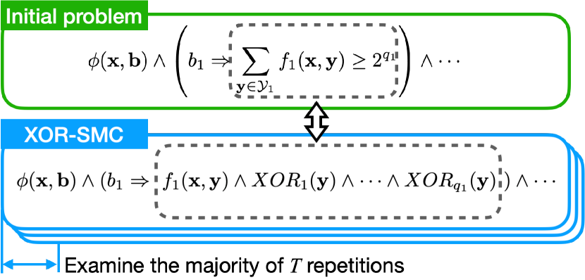
In practice, to reduce the error probability the determination of the model count needs to rely on the majority satisfiability status of a series of equations (4) (instead of a single one). Hence we develop Algorithm 2, which is a little bit more complex than the high-level idea discussed above. The idea is still to transform the highly intractable SMC problem into solving an SAT problem of its polynomial size, while ensuring a constant approximation guarantee. Fig. 1 displays the encoding of Algorithm 2. We can see the core is still to replace the intractable model counting with satisfiability problems subject to randomized constraints. We prove - has a constant approximation guarantee in Theorem 2. We leave the implementation of - in the Appendix B.
Theorem 2.
Let and . Select , we have
-
•
Suppose there exists and , such that is true. In other words,
Then algorithm - (, , , ) returns true with probability greater than .
-
•
Contrarily, suppose is not satisfiable. In other words, for all and ,
then - (, , , ) returns false with probability greater than .
Proof.
Claim 1: Suppose there exists and , such that
| (6) |
holds true. Denote as the number of non-zero bits in . Without losing generality, suppose those non-zero bits are the first bits, i.e., and . Then Eq. (6) can be simplified to:
| (7) |
Consider the Boolean formula defined in the - algorithm (choosing any ). can be simplified by substituting the values of and . After simplification, we obtain:
Let . Observing that . According to Lemma 1, with probability at least , there exists , such that renders true. The probability that is true under is:
Define as a binary indicator variable where
Therefore . when . - returns true if the majority of are true; that is, . Let’s define
When , observing that , we can apply the Chernoff-Hoeffding theorem to obtain:
For , it follows that . Therefore, with a probability at least , we have . In this scenario, - (, , , ) returns true as it discovers , , , for which the majority of Boolean formulae in are true.
Claim 2: Suppose for all and ,
Consider a fixed and , the previous condition with high probability renders most false in Algorithm 2. We prove that the probability is sufficiently low such that - will return false with a high probability after examining all and . The detailed proof is left in Appendix A. ∎
5 Experiment 1: Locate Emergency Shelters
Problem Formulation. Disasters such as hurricanes and floods continue to endanger millions of lives. Shelters are safe zones that protect residents from possible damage, and evacuation routes are the paths from resident zones toward shelter areas. To enable the timely evacuation of resident zones, picking a set of shelter locations with sufficient routing from resident areas should be considered. Given the unpredictability of chaos during natural disasters, it is crucial to guarantee multiple paths rather than one path from residential areas to shelters. This ensures that even if one route is obstructed, residents have alternative paths to safety areas.
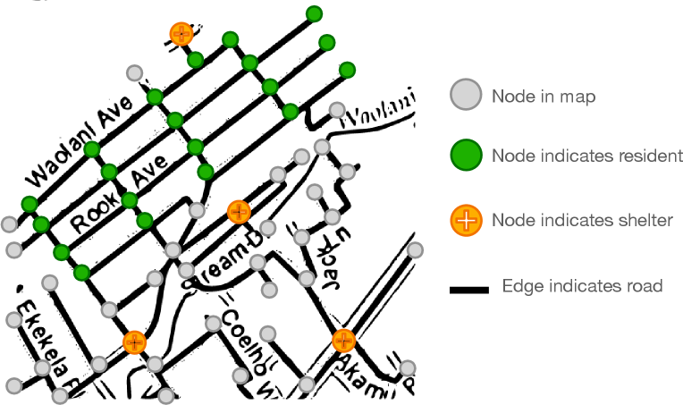
Given a map where nodes in represent areas and an edge indicates a road from to , and denote the number of nodes and edges, respectively. Given a subset of nodes indicates the residential areas, the task is to choose at most nodes as shelters from the rest of the nodes, such that the number of routes that can reach a shelter from each residential area is maximized. Fig. 2 gives an example with shelters and there are sufficiently many roads connecting the resident area to those shelters.
Current methods (Bayram and Yaman 2018; Amideo, Scaparra, and Kotiadis 2019) considered finding shelter locations that have at least one single path from a residential area. However, those proposed methods cannot be generalized to solve the problem that requires sufficient alternative routes from residential area to shelters, primarily because counting the number of paths is intractable. This complexity makes it difficult to solve large-scale problems of this type.
SMC Formulation. - transforms this optimization problem into a decision problem by gradually increasing the path count threshold . The decision problem decides if there are at least paths connecting any residential area with a shelter. The assigned shelters is represented by a vector , where implies node is chosen as shelter. Let represent there are at most shelters. Let be an indicator function that returns one if and only if the selected edges form a path from to . The whole formula is:
We leave the details implementation of in the Appendix C.
Empirical Experiment Analysis
Experiment Setting. We crawl the real-world dataset from the Hawaii Statewide GIS Program website. We extract the real Hawaii map with those major roads and manually label those resident areas on the map. We create problems of different scales by subtracting different sub-regions from the map. 3 major resident areas are picked as , and set .
| Graph Size | |||
|---|---|---|---|
| - (ours) | |||
| GibbsSampler-LS | |||
| QuickSampler-LS | |||
| Unigen-LS | |||
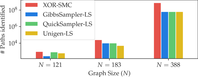
In terms of baselines, we consider the local search algorithm with shelter locations as the state and the number of paths between shelters and resident areas as the heuristic. Due to the intractability of path counting in our formulation, the heuristic is approximated by querying sampling oracles. In particular, we consider 1) Gibbs sampling-based (Geman and Geman 1984) Local Search (Gibbs-LS). 2) Uniform SAT sampler-based (Soos, Gocht, and Meel 2020) Local Search (Unigen-LS). 3) Quick Sampler-based (Dutra et al. 2018) Local Search (Quick-LS). Each baseline runs 5 times, and the best result is included. Each run is until the approach finds a local minimum. For our -, we give a time limit of 12 hours. The algorithm repeatedly runs with increasing until it times out. The time shown in Table 1 and the number of paths in Figure 2 correspond to the cumulative time and the best solutions found before the algorithm times out. For the evaluation metrics, we consider 1) the number of paths identified in the predicted plan by each algorithm, and 2) the total running time of the process.
Result Analysis. In terms of running time (in Table 1), - takes less empirical running time than baselines for finding shelter location assignments over different graphs. In Fig. 3, we evaluate the quality of the predicted shelters by counting the number of connecting paths from residents to the shelters. The path is counted by directly solving the counting predicate by SharpSAT-TD (Korhonen and Järvisalo 2021) with given shelter locations. The shelter locations selected by our - lead to a higher number of paths than those found by the baselines.
| Small Supply Network | Real-world Supply Network | |||||
| Disaster Scale ( of affected edges) | Disaster Scale ( of affected edges) | |||||
| - (ours) | ||||||
| BP-SAA | ||||||
| Gibbs-SAA | ||||||
| IS-SAA | ||||||
| LoopyIS-SAA | ||||||
| Weighted-SAA | ||||||
| Best possible values | ||||||
6 Experiment 2: Robust Supply Chain Design
Problem Formulation. Supply chain management found its importance in operations research and economics. The essence of supply chain management is to integrate the flow of products and finances to maximize value to the consumer. Its importance is underscored by the increasing complexity of business environments, where minor inefficiencies by random disasters result in significant extra costs.
Given a supply chain of suppliers, they form a supply-demand network where each node represents a supplier and edges represent supply-to-demand trades. Each supplier acts as a vendor to downstream suppliers and also as a buyer from upstream suppliers. We assume a conservation of production conditions for each node, i.e., the input-output ratio is 1. To guarantee substantial production, supplier should order necessary raw materials from upstream suppliers in advance. Denote the cost of trade between vendor , and buyer as . Let the amount of goods of the trade between and be and be the total budget to get all his materials ready. Due to unpredictable natural disasters and equipment failure, the trade between and may fail. Denote as the state of different stochastic events, where indicates event occurs. The objective is to design a global trading plan maximizing the expected total production output, accounting for stochastic influences. This is measured by the output of final-tier suppliers, who produce end goods without supplying others.
Existing works in supply chain optimization often gravitate towards mathematical programming approaches. However, when delving into more complex scenarios involving stochastic events—such as uncertain demand or supply disruptions—the task becomes considerably more intricate. Specifically, formulating counting constraints, like guaranteeing a certain amount of supplies across multiple vendors under stochastic events, is intractable. These complexities necessitate innovative approaches that can capture the randomness and dynamism inherent in real-world supply chain systems without sacrificing optimality.
SMC Formulation. Similarly, we transform the maximization into a decision problem by gradually increasing the threshold of the production. Denote the trading plan as , where indicates that purchases raw material from . The decision problem can be formulated into an SMC problem as follows:
| (8) |
where represents final-tier supplier nodes, is a minimum production level to be guaranteed, is the remaining sets of edges after applying trading plan and under the stochastic events of disasters . encodes all essential constraints, e.g., adherence to budget limits, output not exceeding input at each node, etc. We leave the formulation details in Appendix C.
Empirical Experiment Analysis
Experiment Setting. The dataset is the wheat supply chain network from (Zokaee et al. 2017). The dataset only provides the cost of trade, the capacity of transportation, and raw material demand. We further generate stochastic events of disasters (see Appendix C) over different portions of supply-demand edges. The random disasters make the expectation computation intractable. For a better comparison of running time, a small-scale synthetic network is included, in which the cost, budget, and capacities are randomly generated. For the small supply network, the number of nodes in each layer is . For the real-world supply network, the number of nodes in each layer is .
For the baseline, we utilize Sample Average Approximation (SAA)-based methods (Kleywegt, Shapiro, and Homem-de-Mello 2002). These baselines employ Mixed Integer Programming (MIP) to identify a trading plan that directly maximizes the average production across networks impacted by 100 sampled disasters. The average over samples serves as a proxy for the actual expected production. For the sampler, we consider Gibbs sampling (Gibbs-SAA), belief propagation (BP-SAA), importance sampling (IS-SAA), loopy-importance sampling, and weighted sampling (Weighted-SAA). For a fair comparison, we imposed a time limit of 30 seconds for the small-sized network and 2 hours for the real-world network. The time shown in Table 2 for SAA approaches is their actual execution time. Our SMC solver again executes repeatedly with increasing until it times outs. The time shown is the cumulative time it finds the best solution (last one) before the time limit.
To evaluate the efficacy of a trading plan, we calculate its empirical average production under i.i.d. disasters, sampled from the ground-truth distribution. The production numbers are reported in Table 2. This method is adopted due to the computational infeasibility to calculate expectations directly. For SAA approaches that exceed the time limit, the production numbers in Table 2 are for the best solutions found within the time limit.
Result Analysis. Table 2 shows the production and running times of plans derived from various methods. For small networks, while SAA-based methods can complete MIP within the time limit, they remain sub-optimal as they optimize a surrogate expectation derived from sampling, which deviates from the true expectation. In the case of larger networks, these methods further struggle due to the poor scalability of the large MIP formulation. They fail to find good solutions within the 2-hour time limit. In contrast, -, by formulating as an SMC problem, directly optimizes the intractable expectation using XOR counting, and yields superior solution quality and less running time.
7 Conclusion
We presented -, an algorithm with polynomial approximation guarantees to solve the highly intractable Satisfiability Modulo Counting (SMC) problems. Solving SMC problems presents unique challenges due to their intricate nature, integrating statistical inference and symbolic reasoning. Prior work on SMC solving offers no or loose guarantees and may find suboptimal solutions. - transforms the intractable SMC problem into satisfiability problems by replacing intricate model counting with SAT formulae subject to randomized XOR constraints. - also obtains constant approximation guarantees on the solutions obtained. SMC solvers offer useful tools for many real-world problems at the nexus of symbolic and statistical AI. Extensive experiments on two real-world applications in AI for social good demonstrate that - outperforms other approaches in solution quality and running time.
Acknowledgments
We thank all the reviewers for their constructive comments. This research was supported by NSF grant CCF-1918327.
References
- cpm (2023) 2023. AAAI-23 Constraint Programming and Machine Learning Bridge Program.
- nes (2023) 2023. Neuro-symbolic AI for Agent and Multi-Agent Systems (NeSyMAS) Workshop at AAMAS-23.
- Achlioptas and Theodoropoulos (2017) Achlioptas, D.; and Theodoropoulos, P. 2017. Probabilistic Model Counting with Short XORs. In SAT, volume 10491, 3–19. Springer.
- Almeida et al. (2019) Almeida, R.; Shi, Q.; Gomes-Selman, J. M.; Wu, X.; Xue, Y.; Angarita, H.; Barros, N.; Forsberg, B.; García-Villacorta, R.; Hamilton, S.; Melack, J.; Montoya, M.; Perez, G.; Sethi, S.; Gomes, C.; and Flecker, A. 2019. Reducing greenhouse gas emissions of Amazon hydropower with strategic dam planning. Nature Communications, 10.
- Amideo, Scaparra, and Kotiadis (2019) Amideo, A. E.; Scaparra, M. P.; and Kotiadis, K. 2019. Optimising shelter location and evacuation routing operations: The critical issues. Eur. J. Oper. Res., 279(2): 279–295.
- Balog et al. (2017) Balog, M.; Tripuraneni, N.; Ghahramani, Z.; and Weller, A. 2017. Lost Relatives of the Gumbel Trick. In ICML, volume 70, 371–379. PMLR.
- Barbosa et al. (2022) Barbosa, H.; Barrett, C. W.; Brain, M.; Kremer, G.; Lachnitt, H.; Mann, M.; Mohamed, A.; Mohamed, M.; Niemetz, A.; Nötzli, A.; Ozdemir, A.; Preiner, M.; Reynolds, A.; Sheng, Y.; Tinelli, C.; and Zohar, Y. 2022. cvc5: A Versatile and Industrial-Strength SMT Solver. In TACAS, volume 13243, 415–442. Springer.
- Barrett et al. (2009) Barrett, C.; Sebastiani, R.; Seshia, S.; and Tinelli, C. 2009. Satisfiability Modulo Theories, chapter 26, 825–885.
- Barrett et al. (2021) Barrett, C. W.; Sebastiani, R.; Seshia, S. A.; and Tinelli, C. 2021. Satisfiability Modulo Theories. In Handbook of Satisfiability, volume 336, 1267–1329. IOS Press.
- Bayram and Yaman (2018) Bayram, V.; and Yaman, H. 2018. Shelter Location and Evacuation Route Assignment Under Uncertainty: A Benders Decomposition Approach. Transp. Sci., 52(2): 416–436.
- Belanger and McCallum (2016) Belanger, D.; and McCallum, A. 2016. Structured Prediction Energy Networks. In ICML, volume 48, 983–992.
- Biere et al. (2009) Biere, A.; Heule, M. J. H.; van Maaren, H.; and Walsh, T., eds. 2009. Handbook of Satisfiability, volume 185 of Frontiers in Artificial Intelligence and Applications.
- Bjørner et al. (2018) Bjørner, N. S.; de Moura, L.; Nachmanson, L.; and Wintersteiger, C. M. 2018. Programming Z3. In SETSS, volume 11430, 148–201. Springer.
- Braunstein, Mézard, and Zecchina (2005) Braunstein, A.; Mézard, M.; and Zecchina, R. 2005. Survey propagation: an algorithm for satisfiability. Random Struct. Algorithms, 27: 201–226.
- Chakraborty et al. (2014) Chakraborty, S.; Fremont, D. J.; Meel, K. S.; Seshia, S. A.; and Vardi, M. Y. 2014. Distribution-Aware Sampling and Weighted Model Counting for SAT. In AAAI, 1722–1730.
- Chakraborty, Meel, and Vardi (2013) Chakraborty, S.; Meel, K. S.; and Vardi, M. Y. 2013. A Scalable and Nearly Uniform Generator of SAT Witnesses. In CAV, volume 8044, 608–623. Springer.
- Chavira and Darwiche (2008) Chavira, M.; and Darwiche, A. 2008. On probabilistic inference by weighted model counting. Artificial Intelligence, 172(6-7): 772–799.
- Cheng et al. (2012) Cheng, Q.; Chen, F.; Dong, J.; Xu, W.; and Ihler, A. 2012. Approximating the Sum Operation for Marginal-MAP Inference. In AAAI, 1882–1887.
- Choi, Kisa, and Darwiche (2013) Choi, A.; Kisa, D.; and Darwiche, A. 2013. Compiling Probabilistic Graphical Models Using Sentential Decision Diagrams. In ECSQARU, volume 7958, 121–132. Springer.
- Choi, Friedman, and den Broeck (2022) Choi, Y.; Friedman, T.; and den Broeck, G. V. 2022. Solving Marginal MAP Exactly by Probabilistic Circuit Transformations. In AISTATS, volume 151, 10196–10208. PMLR.
- Conitzer and Sandholm (2006) Conitzer, V.; and Sandholm, T. 2006. Computing the optimal strategy to commit to. In EC, 82–90. ACM.
- Conrad et al. (2012) Conrad, J.; Gomes, C. P.; van Hoeve, W.-J.; Sabharwal, A.; and Suter, J. F. 2012. Wildlife corridors as a connected subgraph problem. Journal of Environmental Economics and Management, 63(1).
- Darwiche and Marquis (2002) Darwiche, A.; and Marquis, P. 2002. A Knowledge Compilation Map. J. Artif. Int. Res.
- de Moura and Bjørner (2007) de Moura, L. M.; and Bjørner, N. S. 2007. Efficient E-Matching for SMT Solvers. In CADE, volume 4603 of Lecture Notes in Computer Science, 183–198. Springer.
- de Moura and Bjørner (2008) de Moura, L. M.; and Bjørner, N. S. 2008. Z3: An Efficient SMT Solver. In TACAS, volume 4963, 337–340. Springer.
- Dilkina and Gomes (2010) Dilkina, B.; and Gomes, C. P. 2010. Solving Connected Subgraph Problems in Wildlife Conservation. In CPAIOR, 102–116.
- Dutra et al. (2018) Dutra, R.; Laeufer, K.; Bachrach, J.; and Sen, K. 2018. Efficient sampling of SAT solutions for testing. In ICSE, 549–559. ACM.
- Dyer and Stougie (2006) Dyer, M. E.; and Stougie, L. 2006. Computational complexity of stochastic programming problems. Math. Program., 106(3): 423–432.
- Ermon et al. (2013a) Ermon, S.; Gomes, C. P.; Sabharwal, A.; and Selman, B. 2013a. Embed and Project: Discrete Sampling with Universal Hashing. In NIPS, 2085–2093.
- Ermon et al. (2013b) Ermon, S.; Gomes, C. P.; Sabharwal, A.; and Selman, B. 2013b. Taming the Curse of Dimensionality: Discrete Integration by Hashing and Optimization. In ICML, volume 28, 334–342.
- Fang, Stone, and Tambe (2015) Fang, F.; Stone, P.; and Tambe, M. 2015. When Security Games Go Green: Designing Defender Strategies to Prevent Poaching and Illegal Fishing. In IJCAI.
- Feser et al. (2020) Feser, J. K.; Madden, S.; Tang, N.; and Solar-Lezama, A. 2020. Deductive optimization of relational data storage. Proc. ACM Program. Lang., 4(OOPSLA): 170:1–170:30.
- Flerova et al. (2011) Flerova, N.; Ihler, E.; Dechter, R.; and Otten, L. 2011. Mini-bucket elimination with moment matching. In NIPS Workshop DISCML.
- Fredrikson and Jha (2014) Fredrikson, M.; and Jha, S. 2014. Satisfiability modulo counting: a new approach for analyzing privacy properties. In CSL-LICS, 42:1–42:10. ACM.
- Geman and Geman (1984) Geman, S.; and Geman, D. 1984. Stochastic Relaxation, Gibbs Distributions, and the Bayesian Restoration of Images. IEEE Trans. Pattern Anal. Mach. Intell., 6(6): 721–741.
- Gogate and Dechter (2007) Gogate, V.; and Dechter, R. 2007. SampleSearch: A Scheme that Searches for Consistent Samples. In AISTATS, volume 2, 147–154.
- Gogate and Dechter (2012) Gogate, V.; and Dechter, R. 2012. Importance sampling-based estimation over AND/OR search spaces for graphical models. Artif. Intell., 184-185: 38–77.
- Gomes, Sabharwal, and Selman (2006a) Gomes, C. P.; Sabharwal, A.; and Selman, B. 2006a. Model Counting: A New Strategy for Obtaining Good Bounds. In AAAI, 54–61.
- Gomes, Sabharwal, and Selman (2006b) Gomes, C. P.; Sabharwal, A.; and Selman, B. 2006b. Near-Uniform Sampling of Combinatorial Spaces Using XOR Constraints. In NIPS, 481–488. MIT Press.
- Hazan and Jaakkola (2012) Hazan, T.; and Jaakkola, T. S. 2012. On the Partition Function and Random Maximum A-Posteriori Perturbations. In ICML.
- Hazan and Shashua (2010) Hazan, T.; and Shashua, A. 2010. Norm-Product Belief Propagation: Primal-Dual Message-Passing for Approximate Inference. IEEE Trans. Inf. Theory, 56(12): 6294–6316.
- Israeli and Wood (2002) Israeli, E.; and Wood, R. K. 2002. Shortest-path network interdiction. Networks: An International Journal, 40(2): 97–111.
- Jang, Gu, and Poole (2017) Jang, E.; Gu, S.; and Poole, B. 2017. Categorical Reparameterization with Gumbel-Softmax. In ICLR (Poster).
- Jerrum and Sinclair (1997) Jerrum, M.; and Sinclair, A. 1997. The Markov chain Monte Carlo method: an approach to approximate counting and integration, 482–520. Boston, MA, USA.
- Jerrum, Valiant, and Vazirani (1986) Jerrum, M.; Valiant, L. G.; and Vazirani, V. V. 1986. Random Generation of Combinatorial Structures from a Uniform Distribution. Theor. Comput. Sci., 43: 169–188.
- Jiang, Rai, and III (2011) Jiang, J.; Rai, P.; and III, H. D. 2011. Message-Passing for Approximate MAP Inference with Latent Variables. In NIPS, 1197–1205.
- K., Shoham, and Gurfinkel (2022) K., H. G. V.; Shoham, S.; and Gurfinkel, A. 2022. Solving constrained Horn clauses modulo algebraic data types and recursive functions. Proc. ACM Program. Lang., 6: 1–29.
- Kempe, Kleinberg, and Tardos (2005) Kempe, D.; Kleinberg, J.; and Tardos, É. 2005. Influential nodes in a diffusion model for social networks. In Automata, languages and programming, 1127–1138. Springer.
- Kisa et al. (2014) Kisa, D.; den Broeck, G. V.; Choi, A.; and Darwiche, A. 2014. Probabilistic Sentential Decision Diagrams. In KR.
- Kiselev and Poupart (2014) Kiselev, I.; and Poupart, P. 2014. Policy optimization by marginal-map probabilistic inference in generative models. In AAMAS, 1611–1612. IFAAMAS/ACM.
- Kleywegt, Shapiro, and Homem-de-Mello (2002) Kleywegt, A. J.; Shapiro, A.; and Homem-de-Mello, T. 2002. The Sample Average Approximation Method for Stochastic Discrete Optimization. SIAM J. Optim., 12(2): 479–502.
- Korhonen and Järvisalo (2021) Korhonen, T.; and Järvisalo, M. 2021. Integrating tree decompositions into decision heuristics of propositional model counters (short paper). In 27th International Conference on Principles and Practice of Constraint Programming (CP 2021). Schloss Dagstuhl-Leibniz-Zentrum für Informatik.
- Kuck et al. (2019) Kuck, J.; Dao, T.; Zhao, S.; Bartan, B.; Sabharwal, A.; and Ermon, S. 2019. Adaptive Hashing for Model Counting. In UAI, volume 115, 271–280. AUAI Press.
- Lee et al. (2016) Lee, J.; Marinescu, R.; Dechter, R.; and Ihler, A. 2016. From Exact to Anytime Solutions for Marginal MAP. In AAAI, 3255–3262.
- Liu and Ihler (2012) Liu, Q.; and Ihler, A. 2012. Belief Propagation for Structured Decision Making. In UAI, 523–532. AUAI Press.
- Liu and Ihler (2013) Liu, Q.; and Ihler, A. T. 2013. Variational algorithms for marginal MAP. Journal of Machine Learning Research, 14.
- Madras (2002) Madras, N. 2002. Lectures on Monte Carlo Methods. American Mathematical Society.
- Maneva, Mossel, and Wainwright (2007) Maneva, E. N.; Mossel, E.; and Wainwright, M. J. 2007. A new look at survey propagation and its generalizations. J. ACM, 54(4): 17.
- Marinescu, Dechter, and Ihler (2014) Marinescu, R.; Dechter, R.; and Ihler, A. T. 2014. AND/OR Search for Marginal MAP. In UAI.
- Mauá and de Campos (2012) Mauá, D. D.; and de Campos, C. P. 2012. Anytime Marginal MAP Inference. In ICML.
- Mei, Jiang, and Tu (2018) Mei, J.; Jiang, Y.; and Tu, K. 2018. Maximum A Posteriori Inference in Sum-Product Networks. In AAAI, 1923–1930.
- Munawar et al. (2023) Munawar, A.; Lenchner, J.; Rossi, F.; Horesh, L.; Gray, A.; and Campbell, M., eds. 2023. IBM Neuro-Symbolic AI Workshop 2023 – Unifying Statistical and Symbolic AI.
- Papandreou and Yuille (2010) Papandreou, G.; and Yuille, A. L. 2010. Gaussian sampling by local perturbations. In NIPS, 1858–1866.
- Papandreou and Yuille (2011) Papandreou, G.; and Yuille, A. L. 2011. Perturb-and-MAP random fields: Using discrete optimization to learn and sample from energy models. In ICCV, 193–200.
- Park and Darwiche (2004) Park, J. D.; and Darwiche, A. 2004. Complexity Results and Approximation Strategies for MAP Explanations. J. Artif. Int. Res.
- Ping, Liu, and Ihler (2015) Ping, W.; Liu, Q.; and Ihler, A. 2015. Decomposition Bounds for Marginal MAP. In NIPS, 3267–3275.
- Rossi, van Beek, and Walsh (2006) Rossi, F.; van Beek, P.; and Walsh, T., eds. 2006. Handbook of Constraint Programming, volume 2. Elsevier.
- Shapiro (2003) Shapiro, A. 2003. Monte Carlo sampling methods. Handbooks in operations research and management science, 10: 353–425.
- Sheldon et al. (2010) Sheldon, D.; Dilkina, B.; Elmachtoub, A. N.; Finseth, R.; Sabharwal, A.; Conrad, J.; Gomes, C. P.; Shmoys, D. B.; Allen, W.; Amundsen, O.; and Vaughan, W. 2010. Maximizing the Spread of Cascades Using Network Design. In UAI, 517–526.
- Sontag et al. (2008) Sontag, D.; Meltzer, T.; Globerson, A.; Jaakkola, T.; and Weiss, Y. 2008. Tightening LP Relaxations for MAP using Message Passing. In UAI, 503–510.
- Soos, Gocht, and Meel (2020) Soos, M.; Gocht, S.; and Meel, K. S. 2020. Tinted, Detached, and Lazy CNF-XOR Solving and Its Applications to Counting and Sampling. In CAV, volume 12224 of Lecture Notes in Computer Science, 463–484. Springer.
- Swamy and Shmoys (2006) Swamy, C.; and Shmoys, D. B. 2006. Approximation Algorithms for 2-Stage Stochastic Optimization Problems. In FSTTCS, volume 4337, 5–19. Springer.
- Valiant and Vazirani (1986) Valiant, L. G.; and Vazirani, V. V. 1986. NP is as Easy as Detecting Unique Solutions. Theor. Comput. Sci., 47(3): 85–93.
- Verweij et al. (2003) Verweij, B.; Ahmed, S.; Kleywegt, A. J.; Nemhauser, G. L.; and Shapiro, A. 2003. The Sample Average Approximation Method Applied to Stochastic Routing Problems: A Computational Study. Comput. Optim. Appl., 24(2-3): 289–333.
- Wainwright, Jaakkola, and Willsky (2003) Wainwright, M. J.; Jaakkola, T. S.; and Willsky, A. S. 2003. Tree-reweighted belief propagation algorithms and approximate ML estimation by pseudo-moment matching. In AISTATS. Society for Artificial Intelligence and Statistics.
- Wainwright and Jordan (2008) Wainwright, M. J.; and Jordan, M. I. 2008. Graphical Models, Exponential Families, and Variational Inference. Found. Trends Mach. Learn., 1(1-2): 1–305.
- Welling and Teh (2003) Welling, M.; and Teh, Y. W. 2003. Approximate inference in Boltzmann machines. Artif. Intell., 143(1): 19–50.
- Williams and Snyder (2005) Williams, J. C.; and Snyder, S. A. 2005. Restoring Habitat Corridors in Fragmented Landscapes using Optimization and Percolation Models. Environmental Modeling and Assessment, 10(3): 239–250.
- Wu et al. (2017) Wu, X.; Kumar, A.; Sheldon, D.; and Zilberstein, S. 2017. Robust Optimization for Tree-Structured Stochastic Network Design. In AAAI, 4545–4551.
- Wu, Sheldon, and Zilberstein (2014) Wu, X.; Sheldon, D.; and Zilberstein, S. 2014. Stochastic Network Design in Bidirected Trees. In NIPS, 882–890.
- Wu, Sheldon, and Zilberstein (2015) Wu, X.; Sheldon, D.; and Zilberstein, S. 2015. Fast Combinatorial Algorithm for Optimizing the Spread of Cascades. In IJCAI, 2655–2661.
- Xue, Fern, and Sheldon (2015) Xue, S.; Fern, A.; and Sheldon, D. 2015. Scheduling Conservation Designs for Maximum Flexibility via Network Cascade Optimization. J. Artif. Intell. Res., 52: 331–360.
- Xue, Choi, and Darwiche (2012) Xue, Y.; Choi, A.; and Darwiche, A. 2012. Basing Decisions on Sentences in Decision Diagrams. In AAAI, 842–849.
- Xue et al. (2016) Xue, Y.; Li, Z.; Ermon, S.; Gomes, C. P.; and Selman, B. 2016. Solving Marginal MAP Problems with NP Oracles and Parity Constraints. In NIPS, 1127–1135.
- Yedidia, Freeman, and Weiss (2000) Yedidia, J. S.; Freeman, W. T.; and Weiss, Y. 2000. Generalized Belief Propagation. In NIPS, 689–695. MIT Press.
- Zokaee et al. (2017) Zokaee, S.; Jabbarzadeh, A.; Fahimnia, B.; and Sadjadi, S. J. 2017. Robust supply chain network design: an optimization model with real world application. Annals of Operations Research, 257: 15–44.
Appendix A Proofs of Theorem 2
Proof of Theorem 2 Claim 2
Suppose for all and , there is
Consider a fixed and , we will examine the probability of not returning true when discovering .
If holds true, then the probability of - (, , , ) not returning true for discovering is one.
Otherwise, when is true, i.e,
| (9) |
Let’s select any . The Boolean formula can be simplified by substituting the values of and :
where is the number of digits that are non-zero in , and .
According to Eq. (9), we define
where . Then according to Lemma 1, with probability at least , renders false for all .
Then the probability of being false under all is
Define as a binary indicator variable where
Upon discovering , - won’t return true if the majority of , are false under for all , that is, . By Chernoff–Hoeffding theorem,
For , it follows that , In this case, with a probability at least , - won’t return true upon discovering and .
Noted that - returns false only if it won’t return true upon discovering any . Therefore, we can write
Proof of Theorem 2
Combining both Claim 1 and 2, we can choose the value such that . This completes the proof.
Appendix B Implementation of -
Our code is attached to the supplementary material. It contains 1) the implementation of our - method 2) the list of datasets, and 3) the implementation of several baseline algorithms.
We use CPLEX solver222https://www.ibm.com/products/ilog-cplex-optimization-studio/cplex-optimizer version 22.1.1 as the NP oracle. We use Python package boolexpr333http://www.boolexpr.org/index.html to process those parts involve logic operations “”.
Computational Pipeline of -
Preprocess
The preprocessing step converts the problem into a standard form as specified in Eq. (3):
The crucial aspects are to guarantee
-
•
, should be properly encoded such that for some . (See example in Shelter Location Assignment.)
-
•
, must be a binary-output function. (See example in Robust Supply Chain Design.)
Formulate a binary-output function into a Boolean Formula
A binary-output function can be formulated into a Boolean formula where and are seen as boolean variables and iff. the boolean formula is satisfiable at .
Although it seems straightforward to use SAT solvers, we found it more efficient to transform the SAT into an equivalent Constraint Programming (CP) problem and query the CPLEX solver after comparison. Due to the interchangeability of CP and SAT, we will keep using the SAT formulation for the following discussion.
Add XOR Constraints
Then we need to add random XOR constraints to the Boolean formula. As an example, an XOR constraint for is
In this , each literal , , and the extra in the end (adding an extra can be seen as negating all literals) has chance of appearance. Following this manner, we will sample multiple XOR constraints for each . The number of XOR constraints for is determined by the logarithm of the corresponding threshold .
After sampling all XOR constraints, we will have a boolean formula:
| (10) | ||||
Repeat and Examine the Majority
Appendix C Experiment Settings
All experiments run on a high-end server with two Sky Lake CPUs @ 2.60GHz, 24 Core, 96 GB RAM.
Shelter Location Assignment
As discussed in the main text, the essential decision problem decides there are at least paths connecting any residential area with a shelter. The assigned shelters is represented by a vector , where implies node is chosen as shelter. Let represent there are at most shelters. Let be an indicator function that returns one if and only if the selected edges form a path from to . The whole formula is:
Path Encoding
The path indicator function is implemented as follows. Any path between 2 nodes can be mapped to a unique flow where the flow along the path is 1 and others are 0. One such unit integer flow can be represented by a binary-valued vector:
where if and only if the amount of flow on edge is 1. Then we can encode every path on the map using . Then we can use a flow indicator function instead in the implementation, where
Then can be implemented by encoding flow constraints.
Shelter Location Encoding
The set of nodes with shelters can be further encoded by a binary vector
where represents a shelter assigned to node , i.e., . For example,
| (11) |
implies we place only 3 shelters on node , , and .
After we properly define the notations of this problem, the shelter location problem can be formulated into an SMC:
| (12) |
If problem (12) holds true for some , then the shelter assignment plan meets the safety requirement. Thus in -, we are actually solving an SAT problem:
where we determine whether there is such a and renders the boolean formula above true.
Dataset
The dataset is from Shelters at Hawaii444https://iu.maps.arcgis.com/apps/Styler/index.html?appid=477fae419a014a3ba7c95cdcb39fd946. The case study for this assignment is from Hawaii and involves Mauna Loa volcano. This map offers an analysis of the most practical locations for emergency shelters for displaced people within 15 minutes of their original locations. Relationships between population, emergency shelters, and high-risk lava flow zones on the islands are analyzed. According to different choices of sub-regions, we extract 3 maps with 121, 186, and 388 nodes representing 3 difficulty levels with 237, 359, and 775 undirected edges, respectively. Those maps are included in the code repository.
Evaluation Metric
Suppose we find a shelter assignment for residential areas . The quality of the assignment is evaluated by the total paths from the resident areas to the chosen shelters, which is computed as:
However, the path counting problem is an intractable problem even if shelter locations are given. We use SharpSAT-TD (Korhonen and Järvisalo 2021) (a model counting solver) to solve each counting predicate separately with given shelter locations.
Choice of Baseline
For baseline methods, shelter locations are found by local search with the shelter assignment as the search state and a path approximation estimation function as
The approximated path counting is achieved by querying approximate sampling oracles including Gibbs Sampler, Unigen Sampler555https://github.com/meelgroup/unigen, Quick sampler666https://github.com/RafaelTupynamba/quicksampler, etc.
Hyper Parameters
For all experiments, residential nodes are picked at node , , . The maximum number of shelters is . Parameter (for repeat experiments) is set to be 2, which empirically works well.
Due to the sensitivity of local search to the search state initialization. We initialize the starting point randomly and repeat 5 times. Each run is until the approach finds a local minimum and only those best are picked for comparison. For our -, we give a time limit of 12 hours. The algorithm repeatedly runs with increasing until it times out. The time shown in Table 1 and the number of paths in Figure 2 correspond to the cumulative time and the best solutions found before the algorithm times out.
Robust Supply Chain Design

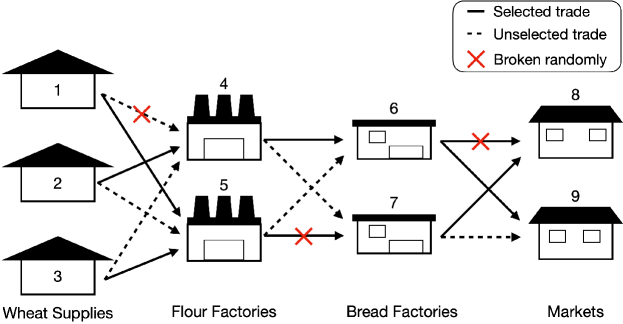
Figure 4 shows an example of the supply chain design. This supply chain (network) can be formulated into a directed acyclic graph . For each node in the supply chain, (1) it represents a supplier, which consumes raw materials from upper-stream suppliers (nodes in the previous layer) and supplies products to down-stream suppliers (nodes in the following layer). The number of nodes is . (2) Each node has a limited budget, denoted by , representing the maximum budget it can spend on purchasing raw materials. (3) We call those nodes without upstream suppliers in the initial graph ”primary suppliers”, e.g., nodes 1 and 2 in Fig. 4. Those without downstream suppliers are called ”final-tier suppliers”, e.g., nodes 5 and 6 in Fig. 4.
For each edge in the graph, (1) it represents the possible trades from nodes to , and the direction is from a supplier to a demand. The number of edges is denoted as . (2) Each edge has a capacity representing the maximum amount of raw materials that can flow from the supplier to the demand. (3) Each edge has a cost for the demander, denoted by . It represents the cost of the trade (mainly from purchase and transportation). (4) The actual amount of goods flow on each edge could be below the capacity, we use to denote the actual flow on edge .
Due to the limited budget, each node can only trade with a limited number of suppliers. Denote this selection as where if and only if the trading edge is selected. The trade selection is shown in Figure 4 (i), and the resulting graph is Figure 4 (b). We have to ensure for all .
A disaster is defined as: where iff. the disaster destroies edge . The disaster is associated with a random distribution . The random disaster happens after the trade selection. An example is in Figure 4 (ii) and (c). In our study, we address the complex scenario where a disaster might simultaneously affect multiple trades, especially those located within the same geographical region, e.g., a wheat factory and a bread market in the same city are likely to face the same natural disaster. Bayesian Networks are exceptionally expressive and capable of effectively representing conditional dependencies and probabilistic relationships among various entities. This makes them particularly well-suited for capturing the nuanced interdependencies among trades. By modeling as a Bayesian Network, we can more accurately reflect the real-world scenario thus providing a more realistic case study analysis.
Problem Formulation
As discussed in the main text Eq. (8), the core decision problem to determine if there is a trading plan that satisfies
where the summation inside the expectation quantifies all incoming raw materials transported to on the actual trading map following trade selection and random disaster , and the total expectation term represents the expected production of node subject to disaster distribution. captures the budget limitation for all node .
Note that if the flow on each edge can vary arbitrarily between 0 and , then a representation of must be included among the decision variables alongside . This is because the same graph can have varying amounts and assignments of flow. As a result, the decision problem becomes overly complex, as encoding for all possible graphs requires exponential space.
To simplify, we assume that all suppliers, except for the primary and final-tier suppliers, are capable of meeting the maximum production requirement with a single incoming trade, that is, . Consequently, the amount of flow on selected trading edges must be full to ensure the maximum flow. Therefore, we can get rid of and consider directly.
SMC Formulation
After simplification, we can expand the decision problem in Eq. (8) as
where is an indicator function, which is defined as follows:
Implementation of -
To utilize -, we need to transform into a sum over 0/1 output function (Boolean formula).
-
•
Discretize Probability: First, let’s discretize . Suppose we use 4 digits to represent probability from to . Then we have,
(13) We model as a Bayesian Network, i.e., where and are two subset of random variables of .
(14) In addition, we need to code up each factor in the Bayesian network, which has a form of or in CPLEX. Use as an example, we need a CPLEX IloNumExpr-typed numerical expression that takes the value assignment of as input and outputs the value of .
For a clear demonstration, assume we have a factor as in Tab. 3. Then we can encode it in CPLEX as:
Table 3: Factor 0 0 0 1 1 0 1 1 where are assisting variables. Then a corresponding indicator function can be implemented as
-
•
Discretize Capacity: The same idea applies to capacity as well. Now we will discretize as a whole. Assume this total capacity can be represented by a 6-digit binary number .
-
•
Practical example of : This indicator function indicates whether edge is in some path from one primary supplier to .
Use Figure 4(a) as an example. Set and examine .
-
•
Overall: After discretization and transformation, the problem is a typical #SAT problem.
where are binary variables introduced by discretizing probability and capacity.
Dataset
We evaluate our algorithm on a real-world wheat supply chain network from (Zokaee et al. 2017), the structure of the supply chain is shown in Fig. 5. For a better comparison, one small-scale synthetic network, in which the parameters are generated with a Gaussian distribution fitted from the real-world data. The statistics of the two supply chain networks are in Table 4.
| Wheat suppliers | Flour factories | Bread factories | Markets | |
|---|---|---|---|---|
| Real-world supply network | 9 | 7 | 9 | 19 |
| Small synthesized supply network | 4 | 4 | 5 | 5 |
In our experiments, we consider different rates of disasters over the supply chain network. We randomly pick 10%, 20%, 30% of edges over the total edges in the network. In each disaster distribution, The joint probability over affected edges is defined as a randomly generated Bayesian Network.
Evaluation Metric
To evaluate the efficacy of a trading plan, we calculate its empirical average of actual production under i.i.d. disasters, denoted as , sampled from the ground-truth distribution. This method is adopted due to the computational infeasibility of directly calculating expectations. Formally, given a trading plan , the performance of is evaluated by
Choice of Baseline
For the baseline, we utilize Sample Average Approximation (SAA)-based methods (Kleywegt, Shapiro, and Homem-de-Mello 2002). These baselines employ Mixed Integer Programming (MIP) to identify a trading plan that directly maximizes the average production across networks impacted by 100 sampled disasters. The average over samples serves as a proxy for the actual expected production. For the sampler, we consider Gibbs sampling (Gibbs-SAA), belief propagation (BP-SAA), importance sampling (IS-SAA), loopy-importance sampling, and weighted sampling (Weighted-SAA). For a fair comparison, we imposed a time limit of 30 seconds for the small-sized network and 2 hours for the real-world network. The time shown in Table 2 for SAA approaches is their actual execution time. Our SMC solver again executes repeatedly with increasing until it times outs. The time shown is the cumulative time it finds the best solution (the last one) before the time limit.
Hyper Parameters
Parameter (for repeat experiments) is set to be 2, which is sufficient to show superior performance over baselines. is discretized into 4 bits, and capacity is discretized into 12 bits. In the randomly generated disasters, each Bayesian network node can have at most 8 parents and the number of Bayesian network edges is around half of the maximum possible number. Those disaster distributions as well as the generation script are available in the code repository.