Sparse Cholesky Covariance Parametrization for Recovering Latent Structure in Ordered Data
Abstract
The sparse Cholesky parametrization of the inverse covariance matrix is directly related to Gaussian Bayesian networks. Its counterpart, the covariance Cholesky factorization model, has a natural interpretation as a hidden variable model for ordered signal data. Despite this, it has received little attention so far, with few notable exceptions. To fill this gap, in this paper we focus on arbitrary zero patterns in the Cholesky factor of a covariance matrix. We discuss how these models can also be extended, in analogy with Gaussian Bayesian networks, to data where no apparent order is available. For the ordered scenario, we propose a novel estimation method that is based on matrix loss penalization, as opposed to the existing regression-based approaches. The performance of this sparse model for the Cholesky factor, together with our novel estimator, is assessed in a simulation setting , as well as over spatial and temporal real data where a natural ordering arises among the variables. We give guidelines, based on the empirical results, about which of the methods analysed is more appropriate for each setting.
Keywords Covariance matrix, sparse matrices, regression analysis, graphical model, Gaussian distribution
1 Introduction
The multivariate Gaussian distribution is central in both statistics and machine learning because of its wide applicability and well theoretical behaviour. Whenever it is necessary to reduce model dimension, such as in a high dimensional setting [1] or in graphical models [2, 3], sparsity is imposed in either the covariance matrix or its inverse .
The inverse covariance matrix directly encodes information about partial correlations; therefore, when a zero pattern is present in , it represents absent edges in the undirected graph of a Gaussian Markov network [4, 5]. Furthermore, letting be its Cholesky decomposition, a zero pattern in the lower triangular matrix yields the acyclic digraph associated with a Gaussian Bayesian network [6, 7] model, up to a permutation of the variables [8]. As a result, much of the academic focus has been on sparsity in either the inverse covariance matrix or its Cholesky decomposition [9, 10, 11, 12, 13].
Conversely, a zero pattern in the covariance matrix represents missing edges from the undirected graph of a covariance graph model [14, 15, 16, 17]. However, a structured zero pattern on the Cholesky decomposition of the covariance matrix has only been addressed by few works: [18] and [19]. In [18] the authors briefly analyse zeros in mainly as a tool for better understanding of a higher-level graphical model called covariance chain, which is the main focus of their work. More directly related to our interests is the work of Rothman et al. [19], who directly explore a regression interpretation of the Cholesky factor over the error variables. However, the authors do not address a structured zero pattern directly; instead, they focus on a banding structure for , inspired by the popularity of this estimator for the covariance matrix. In fact, a significant amount of the paper is devoted to analysing the relationship between the covariance matrix, or its inverse, and banded Cholesky factorization.
To fill this gap, in this paper we focus on arbitrary zero patterns in the Cholesky factor of the covariance matrix . We argue how this naturally models scenarios with ordered variables representing noisy inputs from hidden signal sources, see for example [20] where latent brain regions are assumed to influence neural measurements. We discuss how this model could be extended to unordered variables by defining a new Gaussian graphical model over the Cholesky factorization of the covariance matrix. This new graphical model can be thought of as the analogue of a Gaussian Bayesian network, which is defined via sparse factorizations of the inverse covariance matrix. For ordered variables, we propose a novel learning method by directly penalising a matrix loss, in contrast with existing regression-based approaches in the literature [19]. This new estimator is feasible to compute thanks to a simplification of the loss gradient computation similar to the one proposed in [21]. Finally, we empirically assess the model performance in a broad range of experiments, exploring multiple simulation scenarios as well as real data where a natural spatial or temporal order arises between the variables.
The rest of the paper is organized as follows. In Section 2 we introduce the theoretical preliminaries necessary to follow the exposition. Then we detail the proposed sparse model for the Cholesky factor of the covariance matrix , as well as introduce its extension to a Gaussian graphical model, in Section 3. Afterwards, we discuss existing state-of-the-art estimation methods in Section 4, where we also detail our novel penalized matrix loss proposal. We assess the previously explained estimation methods in both simulated and real experiments, whose results are shown in Section 5. Finally, we close the paper in Section 6, discussing the conclusions that can be drawn from the presented work, and also outlining the planned lines of future research. Appendices A.1, A.2 and A.3 are referenced throughout the paper and contain additional material for the interested reader.
2 Theoretical preliminaries
We will denote as the multivariate Gaussian distribution with mean vector and covariance matrix . Since we focus on the zero pattern in , in the following we will set for notational simplicity, without loosing generality. As in the previous section, we will denote the inverse covariance matrix as .
2.1 The inverse covariance matrix and systems of recursive regressions
As we stated previously, the inverse covariance matrix and its decompositions have been thoroughly researched. If is a -variate Gaussian random vector, that is, if , then the upper Cholesky factorization of can be used to model ordered sequences of regressions [7, 9], as follows.
For , and , let denote the vector of regression coefficients of on , with its -th entry being , the coefficient corresponding to variable . We may equivalently write the statistical model for as a system of recursive linear regression equations (also called a linear structural equation model [22]), where for each ,
| (1) |
with independent Gaussian random variables of zero mean and . The above regression system can also be expressed as , where is a strictly lower triangular matrix with entries . Rearranging the previous equation, we obtain
| (2) |
where with the -dimensional identity matrix. Now if we take variances and inverses on Equation (2), we arrive at the upper Cholesky decomposition of the inverse covariance matrix,
| (3) |
where and are upper triangular matrices, and is a diagonal matrix containing the variances of .
Equations (1) and (3) are intimately related: all parameters of the recursive regression system are encoded in the upper Cholesky factorization. Indeed, we have that and the entry of matrix , , is equal to , therefore all the regression coefficients can also be recovered, and is explicitly written as
| (4) |
2.2 The Cholesky decomposition of a covariance matrix
From Equation (2) we could have proceeded differently. Instead of taking variances and then inverses, most suited for analysing ordered sequences of variable regressions and subsequent Gaussian Bayesian networks (GBNs), we could have just taken variances and would have arrived at the Cholesky decomposition of the covariance matrix [19]
| (5) |
where now and are lower triangular.
Observe that Equation (5) is a direct analogue of Equation (3); although now there is not a natural interpretation of entries in terms of regression coefficients. However, we will now show that the entries of are in fact regression coefficients, just over a different conditioning set. Alternative derivations of this result can be found in [23, p. 158] and [18, p. 846]. The one in [23] is computational, based on the sweep matrix operator [24], whereas [18] provides a sketch based on a recursive expression for regression coefficients. We use instead simple identities over partitioned matrices.
Proposition 1.
For and , the entry of matrix , denoted as , is equal to .
Proof.
Furthermore, observe that, since is lower triangular with ones along the diagonal, the last column of is always a vector of zero entries except the last entry, which is . This means, in particular, that for each , and , the -th element of row vector is equal to , which in turn is equal to the -th entry of , . ∎
2.3 The Gaussian Bayesian network model and sparse Cholesky factorizations of
The upper Cholesky factorization in Equation (3) is typically used as a parametrization for GBNs, see, for example, [13, 8, 25]. In the following we will explain why, since this is closely related to the extension of our proposal to a graphical model.
Let be an acyclic digraph, where is the vertex set and is the edge set. Assume that is a topological order of , which means that for all , denoting as the parent set in of node , it holds that . The ordered Markov property of Bayesian networks states that [7]
| (7) |
where stands for conditional independence [26], that is, and are independent given , for any value of . In the multivariate Gaussian distribution, the above conditional independence is equivalent to the regression coefficient being zero (see for example [27]). Since if and only if , then the zero pattern containing absent edges in can be read off from in Equation (3).
Now allow the ancestral order to be arbitrary, and denote as the set of matrices that have positive diagonal and zeros compatible with a given acyclic digraph ; that is, such that if , , then for all . The GBN model can thus be expressed as
| (8) |
Remark 1.
Observe that if follows a GBN model with graph , the parameter matrix of Equation (8) is not the Cholesky factor of . This only occurs when the ancestral order of the nodes in is ; that is, when the variables follow a natural order (the direct analogue of our model).
However, if we denote as the permutation of rows and columns in following the ancestral order of , then is the upper Cholesky factor of .
3 Sparse Cholesky decomposition of the covariance matrix
We will hereby introduce the sparse Cholesky decomposition model for the covariance matrix, which consists of allowing an arbitrary zero pattern in . The entries of are in correspondence with those in and (see Equation (5), ), and therefore sometimes we will indistinctly refer to each of these matrices .
3.1 The regression interpretations for the covariance Cholesky factor
In terms of model estimation, in (Equation (4)) each column corresponds to the parameters of a single recursive regression, whereas each entry of matrix (Equation (6)) corresponds to a different regression model.
Fortunately, [19] gave an alternative regression interpretation for matrix : recalling Equation (2), where the original variables are written as a linear function of the error terms , and unfolding this matrix equation, we obtain
| (9) |
Thus obtaining an analogue of Equation (1), but now instead of regressing the original variables, the regression is performed over the error terms of the ordered recursive regressions in Equation (1).
Remark 2.
The entry of matrix for , , has therefore two interpretations as a regression coefficient:
-
1.
It is the coefficient of the error on the regression of over .
-
2.
It is the coefficient of variable in the regression of over .
Furthermore, from Equations (1) and (9) we have another dual interpretation for variable : it is the error of the regression of onto , but also of onto .
3.2 A hidden variable model interpretation
The sparse Cholesky parametrization of the covariance matrix naturally models a hidden variable structure [28, 29, 30, 31] over ordered Gaussian observables (Equation (2)). Interpreting the error terms as latent signal sources, then the model is a sort of restricted GBN. This interpretation is naturally associated with the first regression coefficients outlined in Remark 2.
The constraints for this GBN that represents our model are:
-
•
All arcs are from hidden variables to the observed ones .
-
•
There is always an arc from to , for all .
-
•
For each , only variables can have arcs to .
Figure 1 represents one such restricted GBN compatible with our model.
3.3 A graphical model extension for unordered variables
In direct analogy with GBNs and Equation (8), we can define a graphical model which is parametrized by a Cholesky factorization, up to a permutation. Let be an arbitrary given acyclic digraph, and denote with its ancestral order. Let be the predecessor set of a node .
Analogous to in GBNs, denote as the set of matrices which have a zero pattern compatible with . By this we mean that if , , then . We may define the Gaussian graphical model (comparable to Equation (8))
| (11) |
Remark 3.
As in the case of GBNs (Remark 1), the parameter matrix in Equation (11) is lower triangular, and thus coincides with the Cholesky factor of , when the variables are already ancestrally ordered. Otherwise, the sparse Cholesky factorization model applies when the ancestral order is known, that is, denoting as the permutation of rows and columns of following , then is the Cholesky factor of .
This extension has a more natural correspondence with the second regression interpretation of Remark 2, which holds after reordering rows and columns of to comply with , as follows. First note that Equation (6) holds for an unordered version of , and thus we have that for . Therefore, we retrieve a sort of ordered Markov property (comparable to Equation (7))
| (12) |
A simple example of an arbitrary graph would be that in Figure 2. In this model, factor would be lower triangular after reordering its rows and columns following the ancestral ordering of the graph, ,
In the example of Figure 1, where variables already exhibit a natural order, the graph that would represent such interactions would be that in Figure 3, whose parameter matrix is already lower triangular (see also Remark 3).
A further study of this graphical model extension is out of the scope of this work, since we focus on naturally ordered variables from hidden signal sources, but we have discussed it here for completeness and interest for future work.
4 Model estimation
We will first review two regression-based existing estimators for this model that can be found in [19], and then will detail our proposed penalized matrix loss estimation method.
4.1 Existing work: Banding and lasso
Throughout this section denote as a sample of size corresponding to variable , where is assumed to follow the regression model of Equation (9).
The banding estimate for builds upon the respective for . The idea is to estimate by standard least squares only the first sub-diagonals of and set the rest to zero. Specifically, if denotes the starting index, with respect to the band parameter , of the -th row vector in matrix , then, letting ,
| (13) | ||||
where is the Euclidean or -norm. In order to ensure positive definiteness of all matrices involved in the computations, must be smaller than [19]. Matrix inherits the band structure from . The main drawback of this banding estimator is the restrictive zero pattern that it imposes. Note also that this method requires previous selection of the parameter .
An alternative to banding which gives more flexibility over the zero pattern is to use lasso regression over Equation (9),
| (14) | ||||
where this time , , and is the -norm and is the penalisation parameter. Observe that such penalty could be replaced with any other sparsity inducing penalty over , for example, [19] discussed also the nested lasso [32] because the sparsity pattern is preserved in the covariance matrix. We have discarded such penalty because we are primarily interested in an arbitrary zero pattern in and not worried about the induced one in .
4.2 Penalized gradient-based learning of the covariance sparse Cholesky factor
The above approaches are based on the regression interpretation of the sparse Cholesky factor model, Equation (9). By contrast, we propose to directly estimate all of the parameters, that is, matrix entries, by solving one optimization problem. This allows for example to recover maximum likelihood estimates, as well as have the potential to be easily extended to the graphical model interpretation (Equation (11)) following an approach similar to [33].
Denote as the parametrization of a covariance matrix with its Cholesky factor (Equation (5)). We propose to learn a sparse model for by solving the following optimization problem
| (15) |
where is a differentiable loss function over covariance matrices, is the penalisation parameter, and is the -norm for matrices, which induces sparsity on [34]. Note that, as in the regression case, the penalty could be replaced with any other sparsity inducing matrix norm. Solving Equation (15) can be done via proximal gradient algorithms, which have optimal convergence rates among first-order methods [34] and are tailored for a convex but also competitive in the non-convex case [21]. In this work we have used two such smooth loss functions: the negative Gaussian log-likelihood and the triangular Frobenious norm.
The negative Gaussian log-likelihood for a sample when is assumed to be zero is [27] proportional to
| (16) |
where is the maximum likelihood estimator for . On the other hand, the Frobenious norm loss that we also consider is
| (17) |
5 Experiments
In all of the experiments we compare the four estimation methods outlined in the previous section: banding (Equation (13)), lasso regressions (Equation (14)), and our two proposed penalized losses (Equation (16)) and (Equation (17)). These four methods will be denoted in the remainder as , , and , respectively. All data was standardized, and therefore in our proposed losses the sample correlation matrix was used instead of . The implementation of our loss optimization methods and can be found in the R [36] package covchol111Version under development: https://github.com/irenecrsn/covchol. The experiments described throughout this section can be reproduced following the instructions and using the code available at the repository https://github.com/irenecrsn/chol-inv..
5.1 Simulation
We have conducted simulation experiments in two different scenarios. First, because as the work of Rothman et al. [19] is the most directly related to our model, we have replicated their simulation setting for completeness. Therein they select three fixed covariance matrices with either a fixed known banded sparsity pattern or no zeros at all. By contrast, in the second experiment we explore how the methods perform when the sparsity pattern is arbitrary.
In both experiments we have measured two statistics in order to assess both model selection (how precise the zero pattern is recovered) and estimation (how numerically close is the retrieved matrix to the original one). These metrics are evaluated over and in the second experiment instead of and , for better comparability with [19]. Specifically, we use the score for evaluating the zero pattern,
| (18) |
where and are the true positive and discovery rate, respectively,
and the induced matrix -norm,
5.1.1 Fixed covariance matrices
The fixed covariance matrices used in the simulations by Rothman et al. [19] are:
-
•
The autoregressive model of order , where the true covariance matrix has entries , with .
-
•
The -banded correlation matrix with entries for , being the set indicator function.
-
•
The dense correlation matrix with in all of its entries except for the diagonal.
Similarly to [19], we use for matrix dimension values ranging from to , and draw from the respective distribution , , a sample of size which allows to visualize both the and scenarios. With this experiment we measure how sparsity inducing methods for learning behave in scenarios which are not specially suited for them, except for and .
Figure 4 shows the results of the aforementioned simulation scenario. The norms are shown in logarithmic scale for a better comparison between the methods, since there were significant disparities.
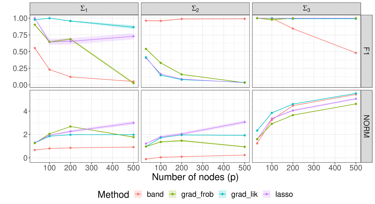
and are both dense matrices, with having entries that decay when moving away from the diagonal. We observe that the inexistent sparsity pattern is best approximated by and , but interestingly and achieve competitive norm results, sometimes even outperforming the rest. Matrix is banded, therefore, as expected, achieves both the highest measure and lowest norm difference.
5.1.2 Arbitrary sparsity pattern in the Cholesky factor
In this experiment the sparse Cholesky factor is simulated using essentially the method of [37, Algorithm 3] with a random acyclic digraph to represent zero pattern, that is, the latent structure (see Figure 1). Observe that in general this does not yield a uniformly sampled Cholesky factor, but it is more flexible that the standard diagonal dominance procedure, see [37] for further discussion on this issue. We generate three Cholesky factors with a proportion of non-zero entries (density/average edge number of the corresponding acyclic digraph), where . Then we draw a sample of size from for ranging between and , as in the previous experiment.
Figure 5 depicts the results.
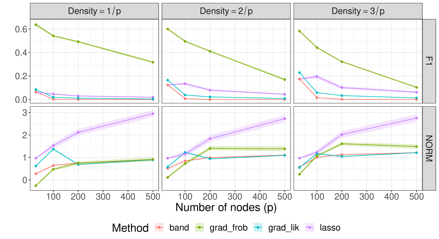
Note that as the density decreases, the score and matrix norm results slightly worsen, but in general the methods behaviour is maintained. The estimator exhibits a performance similar to the previous experiment: although achieving a small score, it has a relatively small matrix norm difference. This behaviour is shared in this case with , which has in general poor performance. However, the worst performing method is , which neither is able to recover the sparsity pattern, nor gets numerically close to the original Cholesky factor (it has a significantly high value for the norm difference). Conversely, method has the best performance, with a significantly high score when compared with the rest and competitive or best norm difference results.
5.2 Real data
In this section we have selected two data sets from the UCI machine learning repository [38] where a natural order arises among the variables, and which are therefore suitable for our sparse covariance Cholesky factorization model. Both of them are labelled with a class variable, therefore after estimating the respective Cholesky factors with each method, we assess classification performance.
For classifying a sample we use quadratic discriminant analysis [19], where is classified in the class value that maximizes
where is the proportion of observations for class and we have expressed in terms of instead of ,
| (19) | ||||
with , and the respective estimates from training samples belonging to class .
Finally, for evaluating classification performance we have used:
-
•
The score, already defined in Equation (18) in terms of and , but adapted to classification instead of matrix entries.
-
•
The true negative rate, , since it is not contained in the score, which is the proportion of observations that have been correctly not classified as class .
-
•
The accuracy, , which measures the proportion of observations that have been correctly assigned a class. Observe that this last metric, unlike the other two, is not class-dependent, but instead global.
5.2.1 Sonar: Mine vs. Rocks
The first real data set we explore is the Connectionist Bench (Sonar, Mines vs. Rocks) data set, which contains numeric observations from a sonar signal bounced at both a metal cylinder (mine) and rocks. It contains variables and observations. Each variable corresponds to the energy within a certain frequency band, integrated over a period of time, in increasing order. Each observation represents a different beam angle for the same object under detection. Over this data set the objective is to classify a sample as rock or mine. This data set was also analysed in [19], but without the expression in terms of for Equation (19) and only using method for .
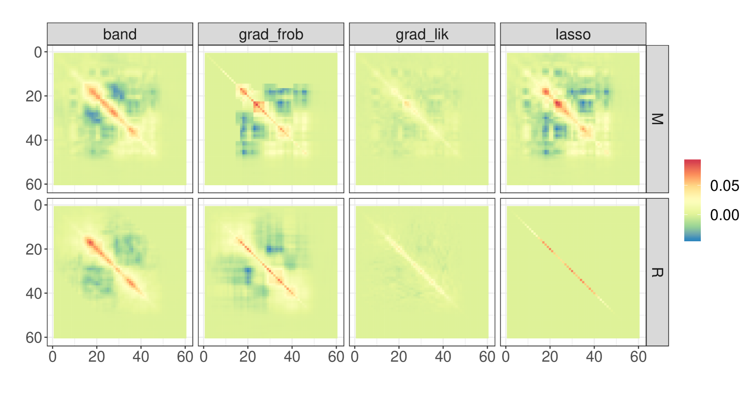
As a first exploratory step, we have applied each of the methods for learning the Cholesky factor to all the instances labelled as (mines), and (rocks), which we show as a heatmap in Figure 6.
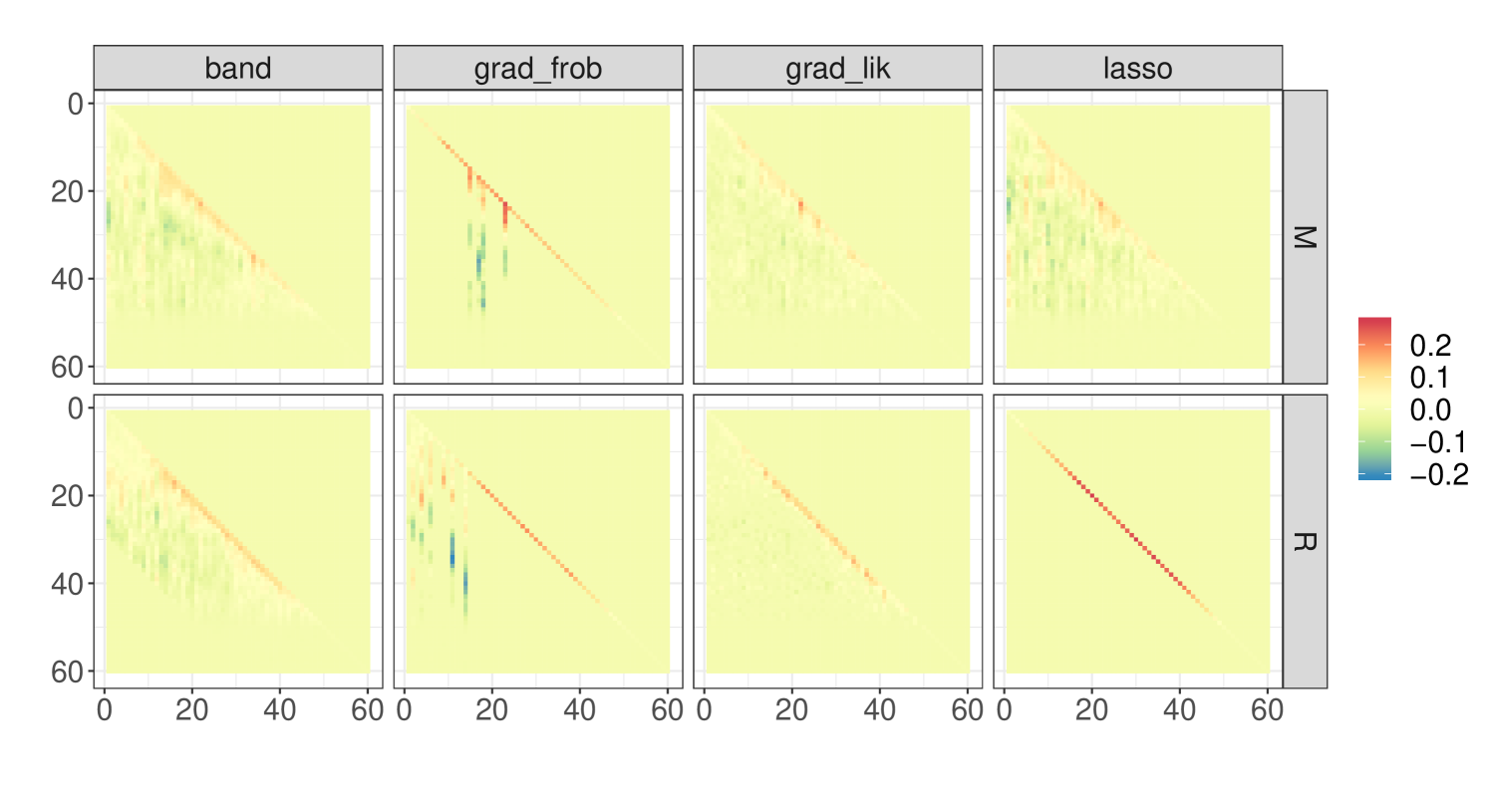
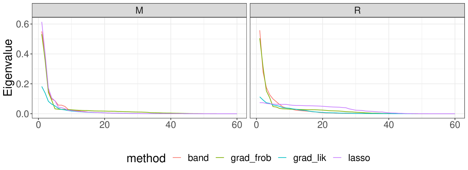
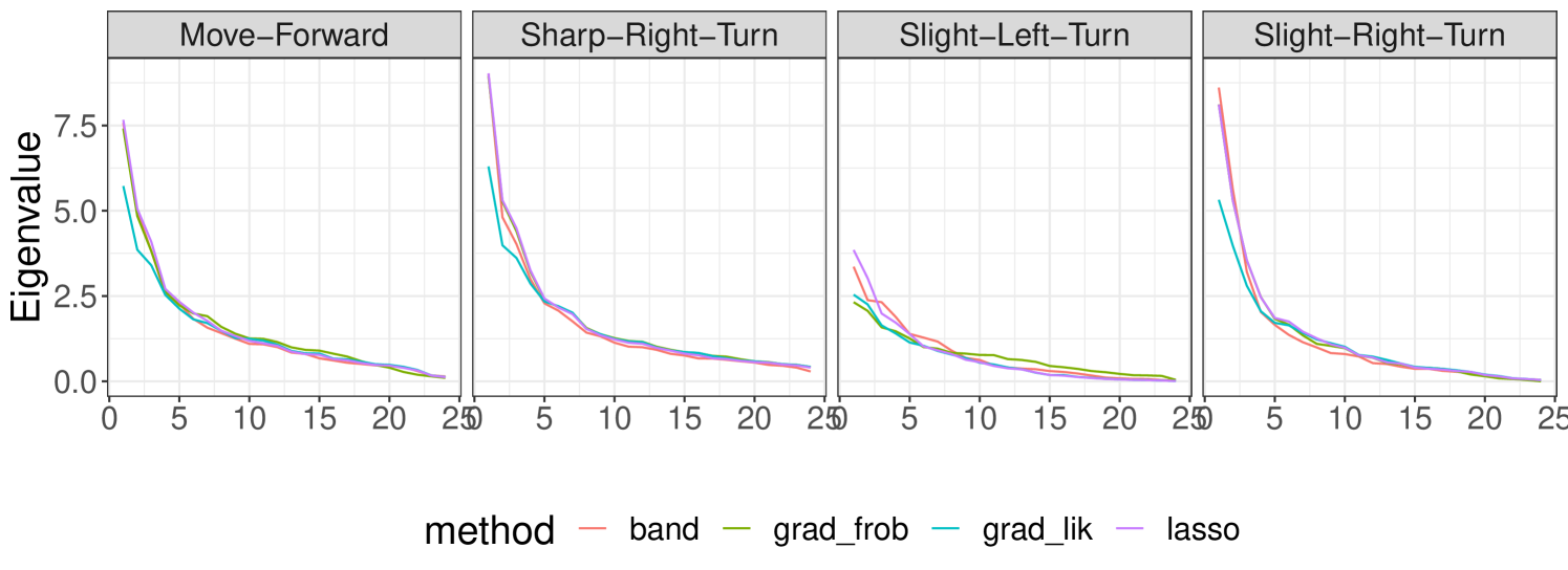
The Cholesky factor for mines retrieved by and look fairly similar, whereas the one for rocks that estimates is nearly diagonal. Bands can be clearly observed from heatmaps by , and all methods impose zero values for variables near to or higher than , which could be motivated by the problem characteristics and hint at high sonar frequencies being nearly noiseless. This latter behaviour is inherited by the covariance matrices, whose heatmaps are shown in Appendix A.3, Figure 9. The entries in the Cholesky factor estimated by are the most extreme, since most of them are zero, and the ones which are not have the highest and lowest values among all the estimates recovered. Despite the outlined differences among the Cholesky factors, the induced covariance matrices exhibit rather similar heatmaps and eigenvalues (Figures 9 and 10 in Appendix A.3).
For the quadratic discriminant analysis we have used leave-one-out cross-validation, since the sample size was sufficiently small to allow it. Table 1 contains the results thus obtained. We see that is the method that performs poorest overall. Conversely, is arguably the best for this problem, except for the of rock samples, which is highest for . However, observing the rest of statistics for , it can be deduced that this method over-classifies samples as mines: it has the lowest for them. On the other hand, performs competitively for this problem, but is in general outperformed or matched by . Since the sonar behaviour hints at a band structure for the covariance (frequency patterns being related to those close to them), and therefore for its Cholesky factor, the good performance of could be expected.
| (M) | 0.78 | 0.08 | 0.78 | 0.62 |
|---|---|---|---|---|
| (M) | 0.8 | 0.7 | 0.55 | 0.33 |
| (R) | 0.79 | 0.97 | 0.45 | 0.26 |
| (R) | 0.78 | 0.15 | 0.65 | 0.5 |
| 0.79 | 0.56 | 0.61 | 0.43 |
5.2.2 Wall-Following Robot Navigation
The other real data set we use is the Wall-Following Robot Navigation one. Here a robot moves in a room following the wall clockwise. It contains observations and variables. Each variable corresponds to the value of an ultrasound sensor, which are arranged circularly over the robot’s body. Here the increasing order reflects the reference angle where the sensor is located. Since the robot is moving clockwise, here the classification task is between four possible class values: Move-Forward, Sharp-Right-Turn, Slight-Left-Turn or Slight-Right-Turn.
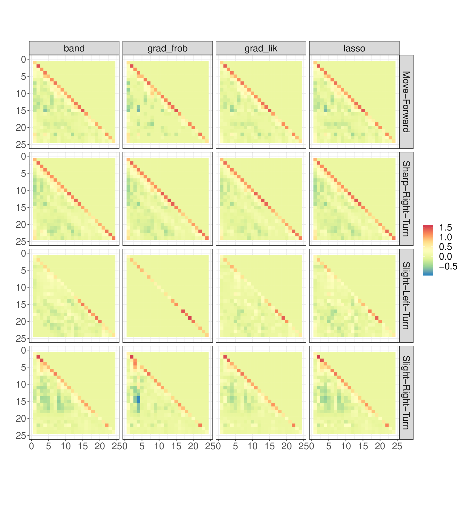
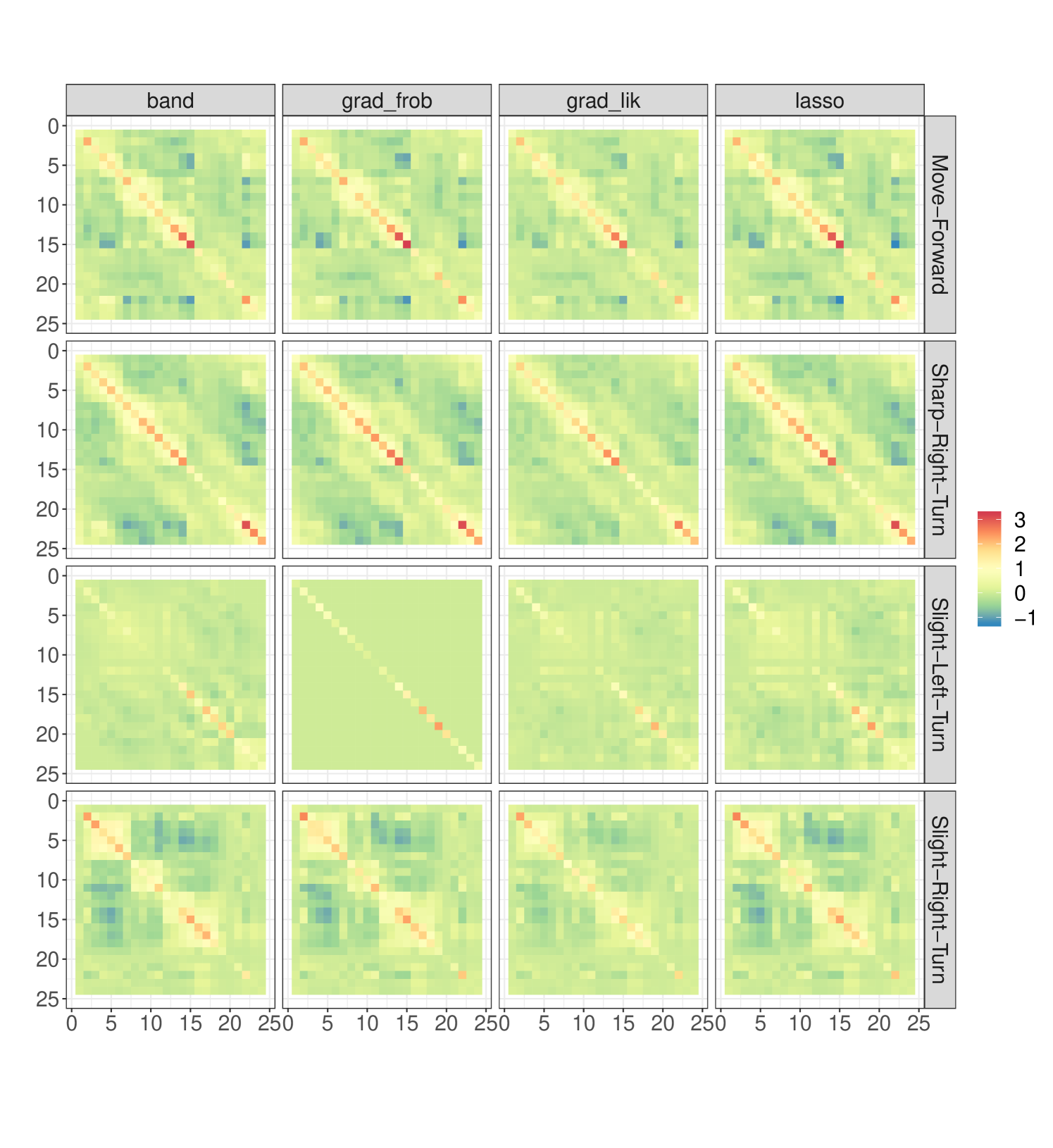
As in the previous problem, we obtain the Cholesky factors for each of the movements, depicted in Figure 7. We notice that outputs a similar matrix (except for the Slight-Left-Turn movement) than the other three methods, which means that the extreme behaviour we observed in the sonar experiment was problem related. By contrast, the Cholesky factor for Slight-Left-Turn is nearly diagonal. The other matrices are rather similar among the methods, with notably choosing in general a high banding parameter (few to no bands). Here we have a similar structure as in the sonar problem: we appreciate for all the movements except Slight-Left-Turn that most entries close to the diagonal are positive, whereas distant ones are frequently negative. Regarding Slight-Left-Turn, these matrices are the sparsest and have near zero values on the diagonal. Since the robot is moving clockwise, this movement is related to obstacles, therefore it could hint that sensor readings are correctly identifying them.
In this problem we have a larger sample size, and therefore we split the data into train and test, with half of the samples on each set. The classification results are shown in Table 2. We observe that all of the methods perform arguably good, in fact they achieve nearly identical accuracy. It is noticeable how competitive are and , which performed much worse in the sonar problem. We also notice that arguably the best results are obtained for the Slight-Left-Turn movement, which confirms our previous intuition over the heatmaps about sensors correctly identifying obstacles. The worst performance over all methods is for the Slight-Right-Turn movement, but is not noteworthy when compared with the rest (except for Slight-Left-Turn).
| (MF) | 0.87 | 0.86 | 0.85 | 0.84 |
|---|---|---|---|---|
| (MF) | 0.64 | 0.64 | 0.61 | 0.62 |
| (SHR) | 0.89 | 0.88 | 0.87 | 0.85 |
| (SHR) | 0.72 | 0.72 | 0.73 | 0.73 |
| (SLL) | 0.96 | 0.95 | 0.98 | 0.98 |
| (SLL) | 0.67 | 0.65 | 0.72 | 0.7 |
| (SLR) | 0.82 | 0.83 | 0.81 | 0.84 |
| (SLR) | 0.56 | 0.57 | 0.55 | 0.57 |
| 0.66 | 0.66 | 0.65 | 0.66 |
5.3 Discussion
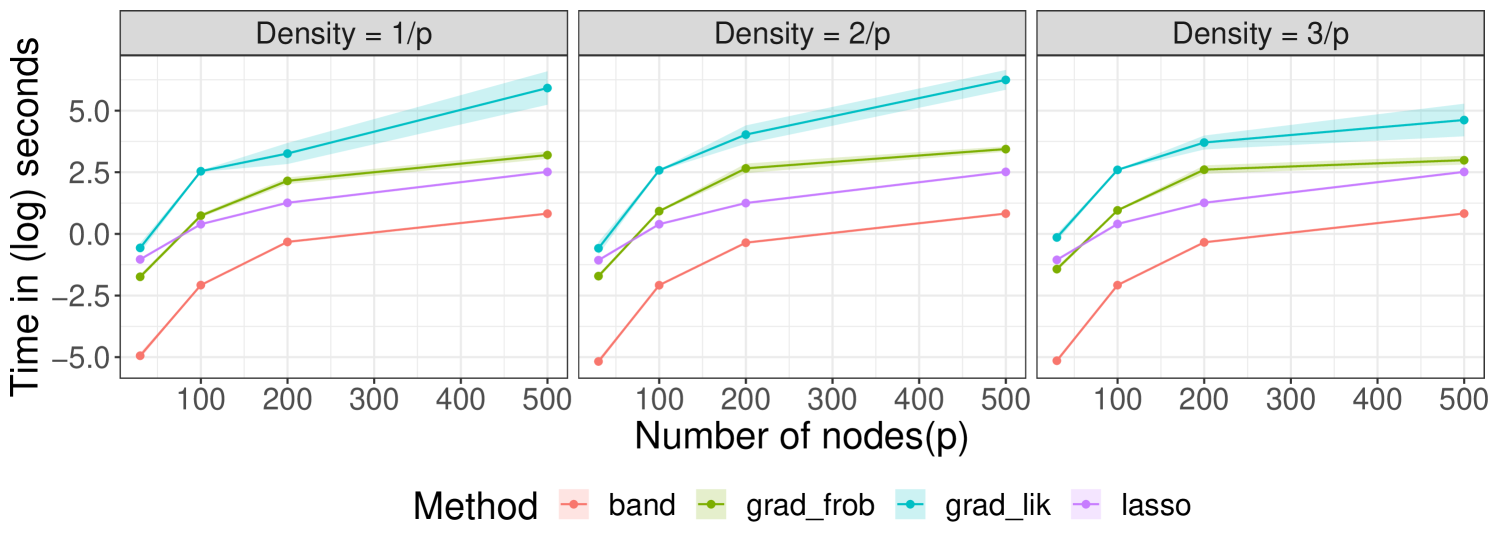
We can draw several conclusions from both the simulated and real experiments. First, we report in Figure 8 the execution time for each method, where it can be seen that is the slowest one and is the fastest.
Whenever there is a clear dependence between variables that are close in the ordering, such as in the sonar example, the method could be preferred, because it is the one that more naturally approximates the structure induced in the Cholesky factor (as happened in the sonar example).
Our new proposed method has shown to be competitive both in execution time as well as recovery results: when interested in model selection, that is, how accurately zeros in the Cholesky factor are estimated, it yields the best results. Conversely, has shown to be the most robust: in simulations it achieved reasonable performance even when the true covariance matrix was dense, and it also performed competitively in the sonar example, which was mostly suited for as we discussed.
Finally, has achieved overall poor results, except for the wall-following robot navigation data set. Specially, in simulations it failed to correctly recover the zero pattern in the Cholesky factor and was the numerically farthest away from the true matrix. Despite this, it is the second fastest of the four methods, so when model selection or robustness are not a concern it is a good alternative to , since it provides more flexibility over the zero pattern in the Cholesky factor.
6 Conclusions and future work
In this paper we have proposed a sparse model for the Cholesky factor of the covariance matrix of a multivariate Gaussian distribution. Few other works in the literature have previously addressed this problem, and we expand them in many ways. We have formalised the extension of an arbitrary zero pattern in the Cholesky factorization to a Gaussian graphical model. We have proposed a novel estimation method that directly optimizes a penalized matrix loss, and we have compared it with the other already existing regression-based approaches in different simulation and real experiments. We have finally discussed which estimation method is preferable depending on the problem characteristics, and argue how our estimation proposal is preferable in many scenarios than those already existing.
As future research, the most direct and interesting derivative work would be to further analyse, both theoretically and empirically, the Gaussian graphical model extension to unordered variables of the sparse covariance Cholesky factorization model. Also in this direction, its relationship with the already established covariance graph [14, 15, 16, 17], an undirected graphical model over the covariance matrix, could yield interesting results. Regarding our novel estimation method, we could explore other alternatives to solve the optimization problems that arise from the two losses that we compute in Appendix A.2. For large data sets, the use of deep learning models to find the hidden Cholesky factor could be also explored.
Acknowledgements
This work has been partially supported by the Spanish Ministerio de Ciencia, Innovación y Universidades through the PID2019-109247GB-I00 project. Irene Córdoba has been supported by the predoctoral grant FPU15/03797 from the Spanish Ministerio de Ciencia, Innovación y Universidades. Gherardo Varando has been supported by a research grant (13358) from VILLUM FONDEN. We thank Adam P. Rothman for helpful discussion and code sharing about his work.
Appendix A Appendices
A.1 A transformation between the Cholesky factorizations of and
The following result gives how to obtain the elements of from those in . Recall that, since is diagonal, the entry in is .
Proposition.
For each with the following identity holds:
Proof.
First we recall that and . Thus, for each and each , if we multiply the -th row in with the -th column of , this must be equal to . Specifically, we obtain the following equation,
Therefore,
which yields the desired result. ∎
A.2 Proximal gradient algorithm and gradient computations for and
We will show how to obtain a simplified expression for the gradient of with respect to as a function of the one with respect to . We will denote these gradients as and , respectively.
Proposition.
For any differentiable loss function ,
| (20) |
Proof.
This proof follows some ideas from [21, Proposition 2.1]. By matrix calculus [39], we have the following gradient expression for ,
| (21) |
where we have used that is symmetric. Furthermore, note that[39]
where () has its () entry equal to one and zero elsewhere. Then from Equation (21) we have
Since for any matrix , we have the desired result. ∎
The above proposition implies that once a loss function is fixed, it is only necessary to compute in order to obtain . We would then use it for the proximal gradient method (Algorithm 1).
A.3 More figures for real data experiments
References
- [1] P. Bühlmann and S. van de Geer, Statistics for High-Dimensional Data: Methods, Theory and Applications. Springer, 2011.
- [2] M. Maathuis, M. Drton, S. Lauritzen, and M. Wainwright, Eds., Handbook of Graphical Models. CRC Press, 2018.
- [3] T. Li, C. Qian, E. Levina, and J. Zhu, “High-dimensional Gaussian graphical models on network-linked data.” Journal of Machine Learning Research, vol. 21, no. 74, pp. 1–45, 2020.
- [4] A. P. Dempster, “Covariance selection,” Biometrics, vol. 28, no. 1, pp. 157–175, 1972.
- [5] M. Yuan and Y. Lin, “Model selection and estimation in the Gaussian graphical model,” Biometrika, vol. 94, no. 1, pp. 19–35, 2007.
- [6] S. Wright, “The method of path coefficients,” Ann. Math. Stat., vol. 5, no. 3, pp. 161–215, 1934.
- [7] N. Wermuth, “Linear recursive equations, covariance selection, and path analysis,” J. Am. Stat. Assoc., vol. 75, no. 372, pp. 963–972, 1980.
- [8] S. van de Geer and P. Bühlmann, “-penalized maximum likelihood for sparse directed acyclic graphs,” Ann. Stat., vol. 41, no. 2, pp. 536–567, 2013.
- [9] M. Pourahmadi, “Joint mean-covariance models with applications to longitudinal data: Unconstrained parameterisation,” Biometrika, vol. 86, no. 3, pp. 677–690, 1999.
- [10] A. d’Aspremont, O. Banerjee, and L. El Ghaoui, “First-order methods for sparse covariance selection,” SIAM J. Matrix Anal. Appl., vol. 30, no. 1, pp. 56–66, 2008.
- [11] J. Friedman, T. Hastie, and R. Tibshirani, “Sparse inverse covariance estimation with the graphical lasso,” Biostatistics, vol. 9, no. 3, pp. 432–441, 2008.
- [12] A. J. Rothman, P. J. Bickel, E. Levina, and J. Zhu, “Sparse permutation invariant covariance estimation,” Electron. J. Stat., vol. 2, pp. 494–515, 2008.
- [13] I. Córdoba, C. Bielza, and P. Larrañaga, “A review of Gaussian Markov models for conditional independence,” J. Stat. Plan. Inference, vol. 206, pp. 127–144, 2020.
- [14] G. Kauermann, “On a dualization of graphical Gaussian models,” Scand. J. Stat., vol. 23, no. 1, pp. 105–116, 1996.
- [15] D. R. Cox and N. Wermuth, “Linear dependencies represented by chain graphs,” Stat. Sci., vol. 8, no. 3, pp. 204–218, 1993.
- [16] S. Chaudhuri, M. Drton, and T. S. Richardson, “Estimation of a covariance matrix with zeros,” Biometrika, vol. 94, no. 1, pp. 199–216, 2007.
- [17] J. Bien and R. J. Tibshirani, “Sparse estimation of a covariance matrix,” Biometrika, vol. 98, no. 4, pp. 807–820, 2011.
- [18] N. Wermuth, D. Cox, and G. M. Marchetti, “Covariance chains,” Bernoulli, vol. 12, no. 5, pp. 841–862, 2006.
- [19] A. J. Rothman, E. Levina, and J. Zhu, “A new approach to Cholesky-based covariance regularization in high dimensions,” Biometrika, vol. 97, no. 3, pp. 539–550, 2010.
- [20] A. Das, D. Sexton, C. Lainscsek, S. S. Cash, and T. J. Sejnowski, “Characterizing brain connectivity from human electrocorticography recordings with unobserved inputs during epileptic seizures,” Neural Comput., vol. 31, no. 7, pp. 1271–1326, 2019.
- [21] G. Varando and N. R. Hansen, “Graphical continuous Lyapunov models,” in Proceedings of the 36th conference on Uncertainty in Artificial Intelligence. Accepted, 2020, arXiv:2005.10483.
- [22] M. Drton, “Algebraic problems in structural equation modeling,” in The 50th Anniversary of Gröbner Bases. Mathematical Society of Japan, 2018, pp. 35–86.
- [23] A. P. Dempster, Elements of Continuous Multivariate Analysis. Adisson-Wesley, 1969.
- [24] A. E. Beaton, “The use of special matrix operators in statistical calculus,” ETS Research Bulletin Series, vol. 1964, no. 2, pp. i–222, 1964.
- [25] Q. Ye, A. Amini, and Q. Zhou, “Optimizing regularized cholesky score for order-based learning of bayesian networks,” IEEE Transactions on Pattern Analysis and Machine Intelligence, vol. Available online, pp. 1–1, 2020.
- [26] A. P. Dawid, “Conditional independence in statistical theory,” J. R. Stat. Soc. Ser. B Stat. Methodol., vol. 41, no. 1, pp. 1–31, 1979.
- [27] T. W. Anderson, An Introduction to Multivariate Statistical Analysis, 3rd ed. John Wiley & Sons, 2003.
- [28] V. Chandrasekaran, P. A. Parrilo, and A. S. Willsky, “Latent variable graphical model selection via convex optimization,” Ann. Statist., vol. 40, no. 4, pp. 1935–1967, 08 2012.
- [29] D. Yatsenko, K. Josić, A. S. Ecker, E. Froudarakis, R. J. Cotton, and A. S. Tolias, “Improved estimation and interpretation of correlations in neural circuits,” PLOS Computational Biology, vol. 11, no. 3, pp. 1–28, 2015.
- [30] M. Zorzi and R. Sepulchre, “AR identification of latent-variable graphical models,” IEEE Transactions on Automatic Control, vol. 61, no. 9, pp. 2327–2340, 2016.
- [31] S. Basu, X. Li, and G. Michailidis, “Low rank and structured modeling of high-dimensional vector autoregressions,” IEEE Transactions on Signal Processing, vol. 67, no. 5, pp. 1207–1222, 2019.
- [32] E. Levina, A. Rothman, and J. Zhu, “Sparse estimation of large covariance matrices via a nested Lasso penalty,” Ann. Appl. Stat., vol. 2, no. 1, pp. 245–263, 2008.
- [33] X. Zheng, B. Aragam, P. Ravikumar, and E. P. Xing, “DAGs with NO TEARS: Continuous optimization for structure learning,” in Proceedings of the 32nd International Conference on Neural Information Processing Systems. Curran Associates Inc., 2018, p. 9492–9503.
- [34] F. Bach, R. Jenatton, J. Mairal, and G. Obozinski, “Optimization with sparsity-inducing penalties,” Found. Trends Mach. Learn., vol. 4, no. 1, p. 1–106, 2012.
- [35] S. Boyd and L. Vandenberghe, Convex Optimization. Cambridge University Press, 2004.
- [36] R Core Team, R: A Language and Environment for Statistical Computing, R Foundation for Statistical Computing, 2020. [Online]. Available: https://www.R-project.org/
- [37] I. Córdoba, G. Varando, C. Bielza, and P. Larrañaga, “On generating random Gaussian graphical models,” International Journal of Approximate Reasoning, vol. 125, pp. 240–250, 2020.
- [38] D. Dua and C. Graff, “UCI machine learning repository,” 2020. [Online]. Available: http://archive.ics.uci.edu/ml
- [39] K. Petersen and M. Pedersen, The Matrix Cookbook. Technical University of Denmark, 2008.