Sparse dynamical system identification with simultaneous structural parameters and initial condition estimation

Consider the structure identification and parameter estimation problem for homogeneous nonlinear ODE system

where $\boldsymbol{x}(t)\in\mathbb{R}^{d}$ is a $d$-dimensional state vector, $\boldsymbol{g}\left(\cdot\right)$ is an unknown vector function, $\boldsymbol{\beta}\in\mathbb{R}^{p}$ and $\boldsymbol{\eta}\in\mathbb{R}^{d}$ denotes the unknown structural parameters and initial condition, respectively.

In practice, the states are always observed with measurement errors, i.e. the observation equation is

where $\boldsymbol{e}(k)\sim\mathcal{N}(\boldsymbol{0},\boldsymbol{\Sigma})$ is an independent Gaussian noise with mean $\boldsymbol{0}$ and finite variance matrix $\boldsymbol{\Sigma}$. Then, for simplicity of presentation, the $n\times d$-dimensional time-series observations are collectively denoted as $\left[\boldsymbol{y}_{i}\right]_{n\times d}$, where each column $\boldsymbol{y}_{i}$, $1\leq i\leq d$, corresponds to the time-series observations $\left\{y_{i}(t_{k})\right\}_{k=1}^{n}$.

Note that the integral form of state equation (1) is

which allows for the simultaneous estimation of structural parameter $\boldsymbol{\beta}$ and initial condition $\boldsymbol{\eta}$. That is, equation (3) offers an alternative integral SINDy (ISINDy) approach for sparse identification of nonlinear dynamical systems, as shown in Figure 1.

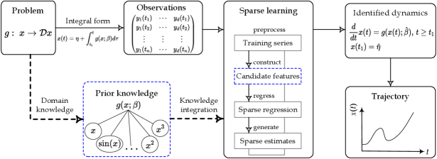
ISINDy depicts learning from a hybrid information source that consists of data and prior knowledge, also belonging to the emerging field known as informed machine learning [27, 28]. The prior knowledge comes from an independent source, such as domain information, empirical experience, and physical laws. The prior knowledge is converted to formal representations — a library of candidate features, which are used to induce an explicit, likely redundancy expression of vector fields. The following sparse learning consists of three steps: preprocessing the time-series observations to estimate noise-free states, determining the candidate features included in the library, and generating estimates from the sparse regression.

Since the observations are contaminated with noise, the penalized spline smoothing [29] is utilized to estimate the states without reference to the state equation. For simplicity of presentation, we treat a single-variable case due to that smoothing is applied to each variable in turn. By using a linear combination of basis functions to approximate $x(t)$, it follows that

where $\boldsymbol{\varphi}(t)=\left[\varphi_{1}(t),\varphi_{2}(t),\cdots,\varphi_{J}(t)\right]^{\top}$ is the known basis function vector, and $\boldsymbol{b}=\left[b_{1},b_{2},\cdots,b_{J}\right]^{\top}$ is the unknown coefficient to be estimated from the observations in equation (2). In order to balance the fitness and smoothness of the fitted curve, the objective function contains a penalized sum of squared errors

where $\rho\in[0,1)$ is a hyper-parameter; at the right hand side, the first term is the squared error criterion measuring the fitness, and the second term is a smoothing penalty measuring the smoothness. The objective function $\mathcal{L}(\boldsymbol{b})$ is a trade-off expression between these two terms: when $\rho=0$, it yields the least-square rough estimates; on the contrary, when $\rho\rightarrow 1$, it yields very smooth estimates and thus nearly linear curve.

Since the basis functions together with their derivatives are known in advance, the penalty term can be reformulated as

where each element of $\boldsymbol{Q}$ is calculated as $Q_{i,j}=\int_{t_{1}}^{t_{n}}{\frac{d^{2}}{dt^{2}}{\varphi}_{i}(t)\frac{d^{2}}{dt^{2}}{\varphi}_{j}(t)}dt$, and these definite integrals can be approximated using the Simpson’s rule. By substituting equation (6) into (5), partially differentiating the objective function with respect to all parameters, in turn, and setting these derivatives to zero, one obtains the estimates of the coefficients and states:

where $\boldsymbol{R}=[\varphi_{j}(t_{k})]$ is an $n\times J$ matrix, $\boldsymbol{y}=\left[y(t_{1}),y(t_{2}),\cdots,y(t_{n})\right]^{\top}$ and $\mathring{\boldsymbol{x}}=\left[\mathring{x}(t_{1}),\mathring{x}(t_{2}),\cdots,\mathring{x}(t_{n})\right]^{\top}$ are both $n\times 1$ column vectors. To tune the hyper-parameter $\rho$, the cross validation criterion [30] is used, i.e. minimizing the generalized cross validation error

where $\boldsymbol{S}(\rho)=\boldsymbol{R}\left[(1-\rho)\boldsymbol{R}^{\top}\boldsymbol{R}+\rho\boldsymbol{Q}\right]^{-1}\boldsymbol{R}^{\top}$ is a $n\times n$ smoothing matrix. It is common to use the grid search strategy to find a reasonable value in the logit scale.

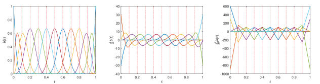
When implementing the penalised spline smoothing, it is vital to select appropriate basis functions. In practice, the basis functions are often chosen as the cubic B-spline basis functions because of their good properties [29, 31]. For example, the property called local compact support, ensures the efficient computation. See Appendix A for details of cubic B-spline basis functions.

From the prior knowledge that the underling dynamics have only a few terms, the vector field $\boldsymbol{g}(\boldsymbol{x};\boldsymbol{\beta})$ is sparse with respect to the candidate feature space $\boldsymbol{\Theta}(\boldsymbol{x})$, i.e.

where $\boldsymbol{\Theta}(\boldsymbol{x})=\left[\theta_{1}(\boldsymbol{x})~{}\theta_{2}(\boldsymbol{x})~{}\cdots~{}\theta_{m}(\boldsymbol{x})\right]$ consists of all possible features and $\boldsymbol{\Xi}\in\mathbb{R}^{m\times d}$ is a sparse matrix having zeros in each column. Subsequently, without loss of generality, each component of $\boldsymbol{g}\left(\boldsymbol{x};\boldsymbol{\beta}\right)$ can be expressed as a linear combination of the candidate features

where $\boldsymbol{\xi}_{i}\in\mathbb{R}^{m}$, $i=1,\cdots,d$, is the $i$th column of the sparse matrix $\boldsymbol{\Xi}$.

By substituting the sparse expression (9) into state equation (3), it follows that

which, by combining equation (10), leads to $d$ separate integral equations

where $\eta_{i}\in\mathbb{R}$ is the $i$th component of initial condition $\boldsymbol{\eta}$. By using the piecewise linear quadrature, the definite integral at each time instant can be approximated as

where $h=t_{k}-t_{k-1}$ is the time interval.

Note that the construction of candidate feature space, $\boldsymbol{\Theta}(\boldsymbol{x})$, is extremely important to guarantee the accuracy of system identification. Ideally, $\boldsymbol{\Theta}(\boldsymbol{x})$ includes all terms in the underlying dynamic system; then, $\boldsymbol{g}(\boldsymbol{x};\boldsymbol{\beta})$ can be well represented as a linear combination of the candidate features. But this is not a simple task due to $\boldsymbol{\Theta}(\boldsymbol{x})$ is not known in advance, even though the prior knowledge can provide some guidance. As a result, it is likely that the number of candidate features, $m$, is large enough to include all possible terms appeared in the vector fields. An alternative strategy is the polynomial and trigonometric functions which has been commonly used in various literature [4].

To illustrate the construction process of $\boldsymbol{\Theta}(\boldsymbol{x})$, we give an example that has three state variables. Denoting the state variable as $\boldsymbol{x}=[x_{1}~{}x_{2}~{}x_{3}]^{\top}$, the 3 linear features are $\theta_{1}(\boldsymbol{x})=x_{1},~{}\theta_{2}(\boldsymbol{x})=x_{2},~{}\theta_{3}(\boldsymbol{x})=x_{3}$; the 6 quadratic features are $\theta_{4}(\boldsymbol{x})=x_{1}x_{1},~{}\theta_{5}(\boldsymbol{x})=x_{1}x_{2},~{}\theta_{6}(\boldsymbol{x})=x_{1}x_{3},~{}\theta_{7}(\boldsymbol{x})=x_{2}x_{2},~{}\theta_{8}(\boldsymbol{x})=x_{2}x_{3},~{}\theta_{9}(\boldsymbol{x})=x_{3}x_{3};$ and, the 10 cubic features are $\theta_{10}(\boldsymbol{x})=x_{1}x_{1}x_{1},~{}\theta_{11}(\boldsymbol{x})=x_{1}x_{1}x_{2},~{}\theta_{12}(\boldsymbol{x})=x_{1}x_{1}x_{3},~{}\theta_{13}(\boldsymbol{x})=x_{1}x_{2}x_{2},~{}\theta_{14}(\boldsymbol{x})=x_{1}x_{2}x_{3},~{}\theta_{15}(\boldsymbol{x})=x_{1}x_{3}x_{3},~{}\theta_{16}(\boldsymbol{x})=x_{2}x_{2}x_{2},~{}\theta_{17}(\boldsymbol{x})=x_{2}x_{2}x_{3},~{}\theta_{18}(\boldsymbol{x})=x_{2}x_{3}x_{3},~{}\theta_{19}(\boldsymbol{x})=x_{3}x_{3}x_{3}$. Likewise, it is easy to show the trigonometric features; the cosine-based ones are $\theta_{20}(\boldsymbol{x})=\cos(\omega x_{1}),~{}\theta_{21}(\boldsymbol{x})=\cos(\omega x_{2}),~{}\theta_{22}(\boldsymbol{x})=\cos(\omega x_{3}),$ where $\omega$ is a hyper-parameter. Finally, we obtain a library of candidate features $\boldsymbol{\Theta}(\boldsymbol{x})=\left[\theta_{\ell}(\boldsymbol{x})\right]$, $\ell=1,\cdots,22$.

Here, if there exists no specific priori knowledge of candidate features, the polynomial functions are suggested because of the following reasons: (1) it is hard to obtain the priori coefficients in the trigonometric functions (see e.g. the hyper-parameter, $\omega$, in $\cos(\omega x_{i})$) and (2) in a finite time interval, there always exists a truncated Taylor series to approximate the vector filed globally.

In the following context, the candidate features are set to polynomial functions unless otherwise stated, that is, $\theta_{\ell}(\boldsymbol{x})=\prod_{i=1}^{d}x_{i}^{r_{i}}$, $1\leq\sum_{i=1}^{d}r_{i}\leq p$, $r_{i}\in\mathbb{N}$, and $p$ is the largest degree of polynomials and traditionally set to be less than 3 for the sake of numerical stability.

Denoting the smoothed time series as a matrix form

and, by using the element-wise product (denoted by $\odot$), we can obtain the data vectors corresponding to the candidate features. For example, if $\theta_{\ell}(\boldsymbol{x})=x_{1}x_{2}x_{3}$, then $\boldsymbol{\theta}_{\ell}(\mathring{\boldsymbol{X}})=\mathring{\boldsymbol{x}}_{1}\odot\mathring{\boldsymbol{x}}_{2}\odot\mathring{\boldsymbol{x}}_{3}$ and subsequently, the data matrix is $\boldsymbol{\Theta}(\mathring{\boldsymbol{X}})=\left[\boldsymbol{\theta}_{1}(\mathring{\boldsymbol{X}}),~{}\cdots,~{}\boldsymbol{\theta}_{m}(\mathring{\boldsymbol{X}})\right]$ and for ease of notation, denoted by $\mathring{\boldsymbol{\Theta}}$.

Substituting data matrices into equation (12) gives a pseudo linear regression whose estimates can be obtained by minimizing the least-square objective function

where $\boldsymbol{S}=\left[\boldsymbol{0},~{}\boldsymbol{I}_{n-1}\right]$ selects the last $n-1$ rows, $\boldsymbol{C}=\frac{h}{2}\left[\boldsymbol{L}_{n-1},~{}\boldsymbol{0}\right]+\frac{h}{2}\left[\boldsymbol{0},~{}\boldsymbol{L}_{n-1}\right]$ denotes the cumulative operation, $\boldsymbol{I}_{n-1}$ is an identity matrix and $\boldsymbol{L}_{n-1}$ is a special left triangular with all the entries above the main diagonal are zero and ones elsewhere. It is easy to show the simultaneous least-square estimates of structural parameters and initial condition are

then, according to the inverse formula of block matrix [32], the inverse matrix can be rewritten as

where

By plugging equation (16) back into (15), we can separate the estimates of structural parameters and initial condition, respectively expressed as

and

Note that all of the the resultant least-square estimates of structural parameters are not equal to zero and thus cannot select the correct model structure, that is, equation (17) always results in a full model including all candidate features. In order to perform structure selection, the objective function (14) is constrained to generate sparse estimates, that is

where $\lambda_{i}\geq 0$ is a hyper-parameter that measures the sparsity of the parameter vector $\boldsymbol{\xi}_{i}$.

By selecting an appropriate hyper-parameter $\lambda_{i}$, equation (19) leads to a parsimonious model structure that balances model complexity with descriptive capability. Equation (19) can be solved by many algorithms, such as the least absolute shrinkage and selection operator (LASSO) [33] and least square approximation (LSA) [34]. Here, we select the sequential threshold least squares (STLS) [35] to generate sparse structural estimates, as shown in Algorithm 1.

Consider the logistic growth equation

with initial condition $x(0)=\eta=0.1$.

The trajectories are generated under the configuration: $t\in[0,6]$ with $h=0.01$, and the noise level $nvr\in[10\%,30\%,50\%]$. When implementing Algorithm 1, the threshold value is set to $\lambda=0.1$. In each noisy scenario, the estimates of sparse structural parameters and initial condition are summarised in Table 1 (Appendix B), and the results show that only the proposed ISINDy identifies the correct active terms together with high-accuracy estimates. By substituting the ISINDy-based estimates and running the ode45 routine, one has the identified trajectories in Figure 2.

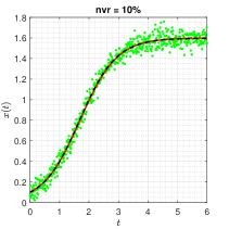
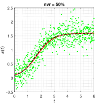
Figure 2 shows that the identified trajectories is very close to the true ones, even though the noise level is as high as $nvr=50\%$, indicating that ISINDy is robust to measurement noises. Moreover, both InSINDy and ISINDy can identify the correct active terms when the noise level is $nvr=10\%$, but ISINDy produces more accurate estimates and as the noise level increases, InSINDy fails to generate correct active terms. For example, when the noise level is $nvr=30\%$, the identified equations of ISINDy and InSINDy are

and

respectively. It is obvious that the InSINDy-based equation includes a redundant active term in the vector field.

Consider the Lokta–Volterra system

with initial condition $[x_{1}(0),x_{2}(0)]^{\top}=[\eta_{1},\eta_{2}]^{\top}=[1.8,1.8]^{\top}$.

The true trajectory are generated under the configuration: $t\in[0,10]$ with $h=0.01$, and the noise level $nvr\in[5\%,10\%,15\%]$. Setting the threshold value to $\lambda=0.3$, the estimates of sparse structural parameters and initial conditions are summarised in Table 2 (Appendix B). The results show that in all three noisy scenarios, only the proposed ISINDy identifies the correct active terms and generates high-accuracy parameter estimates. By substituting these ISINDy-based estimates and running the ode23 routine, one obtains the identified trajectories in Figure 3.

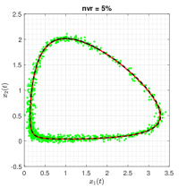
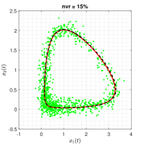
Figure 3 shows that the proposed ISINDy captures the correct active terms in all three noisy scenarios, even though the noise level is up to $nvr=15\%$. Increasing the noise level leads to larger errors in the estimation of structural parameters and initial condition, resulting in more biased trajectories. Besides, to compare the identified and true dynamic systems in the presence of measurement noises on the observations, we simulate the true and identified trajectories at the time range $t\in[0,30]$. Figure 4 shows that the trajectory of the identified dynamical system almost coincides with the true one, indicating that ISINDy can also generate accurate long-term forecasts.

Consider the chaotic Lorenz system

with initial condition $[x_{1}(0),x_{2}(0),x_{3}(0)]^{\top}=[\eta_{1},\eta_{2},\eta_{3}]^{\top}=[-5,10,30]^{\top}$.

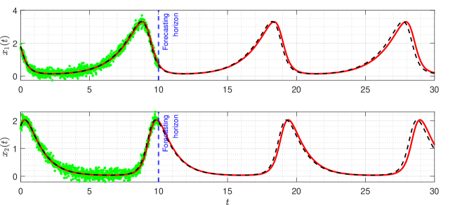
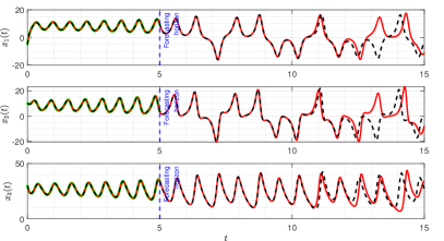
The true trajectories are generated under the configuration: $t\in[0,5]$, $h=0.005$, and $nvr\in[5\%,10\%,15\%]$. The threshold value is set to $\lambda=0.8$, and the estimates of sparse structural parameters and initial conditions are summarised in Table 3 (Appendix C). The results show that SINDy, InSINDy, and ISINDy correctly identify the active terms in all three noisy scenarios for the first component, but SINDy and InSINDy fail to identify the correct active terms in the second and third components, letting alone the accurate estimates of parameters. Only ISINDy picks out the correct active terms and generates high-accuracy estimates in all three noisy scenarios. By substituting the ISINDy-based estimates and running the ode45 routine, one obtains the identified trajectories in Figure 5.

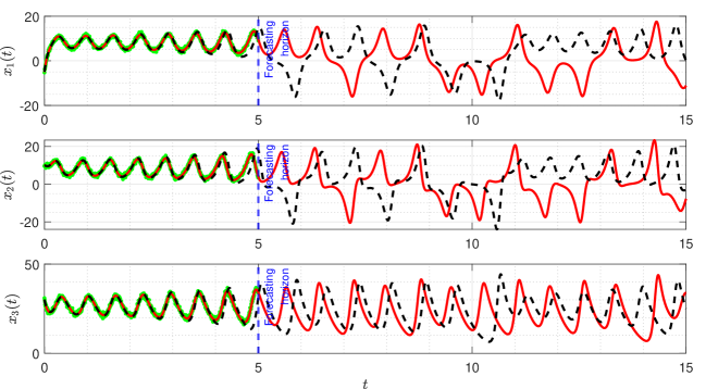
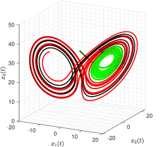
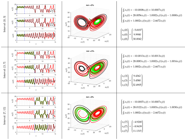
It is worth noting, however, that although the identified equation has correct model structure and also high-accuracy estimates, the identified trajectories may still stray off the true one quickly. For instance, in the $nvr=15\%$ scenario, the trajectories of three state variables are plotted in Figure 6. It is clear that the identified trajectories almost coincides with the true ones for a short time from $t=0$ to about $t=4$ and then stray from about $t=5$ on. The reason for this phenomenon is that Lorenz system has chaotic solutions for certain structural parameters and initial conditions. The identified trajectory is very sensitive to the estimates of structural parameters and initial condition. A small bias on the estimates results in large offsets in the trajectory. Specifically, assuming the observations are noise-free, i.e. $nvr=0$, the identified attractor associated with the trajectories of three states are shown in Figure 7. The identified trajectories starts to fast stray off the true ones from about $t=12$ on, indicating unreliable long-term forecasts even under a noise-free environment.

The results of three cases show that the proposed ISINDy outperforms the standard SINDy and its integral variant InSINDy, in both structure identification and parameter estimation terms. When observations are noise-free, i.e. $nvr=0\%$, all three methods can identify the correct model structure, but the parameter estimates obtained from ISINDy are much closer to their true values than those obtained form SINDy and InSINDy (see Tables 1–3 in Appendix B). To be specific, SINDy and ISINDy outperform InSINDy due to that the formers use a trapezoid formula rather than the Euler’s formula, but this does not hold in noisy scenarios due to that the derivative approximation-based SINDy is sensitive to measurement noises and thus generates poor results, especially in the Lorenz system case (see Table 3 in Appendix B).

It is worth noting, however, that the aforementioned simulations are conducted under two conditions: (1) the time range is fixed in a specified interval, and (2) the candidate features include all possible terms appearing in vector fields. Actually, these two factors have important effects on the performance of ISINDy.

1. (i)

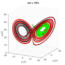
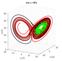
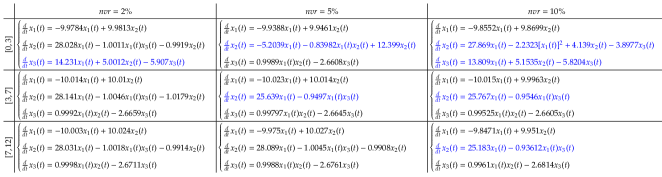
   For factor (1), taking the Lorenz system as an example, the fixed time interval is set to $[0,3]$, $[3,7]$, and $[7,12]$, respectively. When the observations are noise-free, ISINDy identifies the correct model structure in all three time interval settings (see Figure 9 in Appendix C). But, when the observations are contaminated by noises, the noise robustness of ISINDy in each interval is different. Figure 10 in Appendix C shows that ISINDy generates wrong model structure when $nvr=2\%$, indicating that in $[0,3]$ the noise tolerance is less than 2%. Similarly, in $[3,7]$ the noise tolerance is less than 5% and in $[7,12]$ the noise tolerance is less than 10%. An alternative strategy to improve robustness is guaranteeing the quality of smoothing, which is inferred from the noise-free observations cases.

2. (ii)

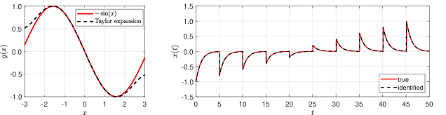
   For factor (2), a simple ODE $\frac{d}{dt}x=-\sin(x)$ is employed to explore the effect of candidate features on identification accuracy. Note that the Taylor expansion of the vector field is

   $$g(x)=-\sin(x)=-x+\frac{1}{3!}x^{3}-\frac{1}{5!}x^{5}+\mathcal{O}(x^{7})=-x+0.16667x^{3}-0.0083x^{5}+\mathcal{O}(x^{7}).$$

   On this test problem, ISINDy with different candidate features is investigated, including polynomial, trigonometric, and a combination of both, shown in Table 4 (Appendix D). In the case of polynomial features, the degree of polynomial is set to 3 and 5 in turn, and in both settings ISINDy identifies the correct active terms together with high-accuracy parameters in the Taylor expansion of $-\sin(x)$. In both of the other cases of trigonometric features or a combination of polynomial and trigonometric features, the correct active term $\sin(x)$ is identified.

Furthermore, the time interval and the design of candidate features always interact. Taking the simple ODE $\frac{d}{dt}x=-\sin(x)$ as an example, in the time range of $t\in[0,5]$, the resulting trajectories lie in the range of $x(t)\in[-1.0,1.0]$. This guarantees that the Taylor series expansion can approximate the vector filed, thereby generating the excellent dynamic reconstruction, as shown in Figure 11 (Appendix D).

References

- Lennart [1999] L. Lennart, System identification: Theory for the user, Prentice Hall PTR, 1999.
- Young [2012] P. C. Young, Recursive estimation and time-series analysis: an introduction for the student and practitioner, 2nd ed., Springer Science & Business Media, 2012.
- Ahsan [2016] Z. Ahsan, Differential equations and their applications, PHI Learning Pvt. Ltd., 2016.
- Brunton and Kutz [2019] S. L. Brunton, J. N. Kutz, Data-driven science and engineering: Machine learning, dynamical systems, and control, Cambridge University Press, 2019.
- Young [2013] P. C. Young, Hypothetico-inductive data-based mechanistic modeling of hydrological systems, Water Resources Research 49 (2013) 915–935.
- Chen et al. [2011] Y. Chen, B. Yang, Q. Meng, Y. Zhao, A. Abraham, Time-series forecasting using a system of ordinary differential equations, Information Sciences 181 (2011) 106–114.
- Bongard and Lipson [2007] J. Bongard, H. Lipson, Automated reverse engineering of nonlinear dynamical systems, Proceedings of the National Academy of Sciences 104 (2007) 9943–9948.
- Schmidt and Lipson [2009] M. Schmidt, H. Lipson, Distilling free-form natural laws from experimental data, Science 324 (2009) 81–85.
- Quade et al. [2016] M. Quade, M. Abel, K. Shafi, R. K. Niven, B. R. Noack, Prediction of dynamical systems by symbolic regression, Physical Review E 94 (2016) 012214.
- Daniels and Nemenman [2015] B. C. Daniels, I. Nemenman, Automated adaptive inference of phenomenological dynamical models, Nature Communications 6 (2015) 1–8.
- Ye et al. [2015] H. Ye, R. J. Beamish, S. M. Glaser, S. C. Grant, C.-h. Hsieh, L. J. Richards, J. T. Schnute, G. Sugihara, Equation-free mechanistic ecosystem forecasting using empirical dynamic modeling, Proceedings of the National Academy of Sciences 112 (2015) E1569–E1576.
- Raissi [2018] M. Raissi, Deep hidden physics models: Deep learning of nonlinear partial differential equations, Journal of Machine Learning Research 19 (2018) 932–955.
- Qin et al. [2019] T. Qin, K. Wu, D. Xiu, Data driven governing equations approximation using deep neural networks, Journal of Computational Physics 395 (2019) 620–635.
- Wang et al. [2016] W.-X. Wang, Y.-C. Lai, C. Grebogi, Data based identification and prediction of nonlinear and complex dynamical systems, Physics Reports 644 (2016) 1–76.
- Tolle et al. [2011] K. M. Tolle, D. S. W. Tansley, A. J. Hey, The fourth paradigm: Data-intensive scientific discovery [point of view], Proceedings of the IEEE 99 (2011) 1334–1337.
- Wang et al. [2011] W.-X. Wang, R. Yang, Y.-C. Lai, V. Kovanis, C. Grebogi, Predicting catastrophes in nonlinear dynamical systems by compressive sensing, Physical Review Letters 106 (2011) 154101.
- Schaeffer et al. [2013] H. Schaeffer, R. Caflisch, C. D. Hauck, S. Osher, Sparse dynamics for partial differential equations, Proceedings of the National Academy of Sciences 110 (2013) 6634–6639.
- Brunton et al. [2016] S. L. Brunton, J. L. Proctor, J. N. Kutz, Discovering governing equations from data by sparse identification of nonlinear dynamical systems, Proceedings of the National Academy of Sciences 113 (2016) 3932–3937.
- Rudy et al. [2017] S. H. Rudy, S. L. Brunton, J. L. Proctor, J. N. Kutz, Data-driven discovery of partial differential equations, Science Advances 3 (2017) e1602614.
- Rudy et al. [2019] S. Rudy, A. Alla, S. L. Brunton, J. N. Kutz, Data-driven identification of parametric partial differential equations, SIAM Journal on Applied Dynamical Systems 18 (2019) 643–660.
- Mangan et al. [2017] N. M. Mangan, J. N. Kutz, S. L. Brunton, J. L. Proctor, Model selection for dynamical systems via sparse regression and information criteria, Proceedings of the Royal Society A: Mathematical, Physical and Engineering Sciences 473 (2017) 20170009.
- Chou and Voit [2009] I.-C. Chou, E. O. Voit, Recent developments in parameter estimation and structure identification of biochemical and genomic systems, Mathematical biosciences 219 (2009) 57–83.
- Ramsay et al. [2007] J. O. Ramsay, G. Hooker, D. Campbell, J. Cao, Parameter estimation for differential equations: a generalized smoothing approach, Journal of the Royal Statistical Society: Series B (Statistical Methodology) 69 (2007) 741–796.
- Ramsay and Hooker [2017] J. Ramsay, G. Hooker, Dynamic data analysis: modeling data with differential equations, Springer Science & Business Media, 2017.
- Dattner and Klaassen [2015] I. Dattner, C. A. J. Klaassen, Optimal rate of direct estimators in systems of ordinary differential equations linear in functions of the parameters, Electronic Journal of Statistics 9 (2015) 1939–1973.
- Schaeffer and McCalla [2017] H. Schaeffer, S. G. McCalla, Sparse model selection via integral terms, Physical Review E 96 (2017) 023302.
- von Rueden et al. [2021] L. von Rueden, S. Mayer, K. Beckh, B. Georgiev, S. Giesselbach, R. Heese, B. Kirsch, J. Pfrommer, A. Pick, R. Ramamurthy, M. Walczak, J. Garcke, C. Bauckhage, J. Schuecker, Informed Machine Learning – A taxonomy and survey of integrating prior knowledge into learning systems, IEEE Transactions on Knowledge and Data Engineering (2021) 1–20.
- Karniadakis et al. [2021] G. E. Karniadakis, I. G. Kevrekidis, L. Lu, P. Perdikaris, S. Wang, L. Yang, Physics-informed machine learning, Nature Reviews Physics 3 (2021) 422–440.
- Cao et al. [2012] J. Cao, J. Cai, L. Wang, Estimating curves and derivatives with parametric penalized spline smoothing, Statistics and Computing 22 (2012) 1059–1067.
- Wahba [1990] G. Wahba, Spline models for observational data, Siam, 1990.
- Patrikalakis and Maekawa [2002] N. M. Patrikalakis, T. Maekawa, Representation of curves and surfaces, in: N. M. Patrikalakis, T. Maekawa (Eds.), Shape Interrogation for Computer Aided Design and Manufacturing, Springer, Berlin, Heidelberg, 2002, pp. 1–33. doi:10.1007/978-3-642-04074-0_1.
- Lu and Shiou [2002] T.-T. Lu, S.-H. Shiou, Inverses of 2 2 block matrices, Computers and Mathematics with Applications 43 (2002) 119–129.
- Tibshirani [2011] R. Tibshirani, Regression shrinkage and selection via the lasso: a retrospective, Journal of the Royal Statistical Society: Series B (Statistical Methodology) 73 (2011) 273–282.
- Wang and Leng [2007] H. Wang, C. Leng, Unified LASSO estimation by least squares approximation, Journal of the American Statistical Association 102 (2007) 1039–1048.
- Zhang and Schaeffer [2019] L. Zhang, H. Schaeffer, On the convergence of the SINDy algorithm, Multiscale Modeling and Simulation 17 (2019) 948–972.
- Delahunt and Kutz [2022] C. B. Delahunt, J. N. Kutz, A toolkit for data-driven discovery of governing equations in high-noise regimes, IEEE Access 10 (2022) 31210–31234.
- Pia Saccomani et al. [2003] M. Pia Saccomani, S. Audoly, L. D’Angiò, Parameter identifiability of nonlinear systems: The role of initial conditions, Automatica 39 (2003) 619–632.
- Miao et al. [2011] H. Miao, X. Xia, A. S. Perelson, H. Wu, On identifiability of nonlinear ODE models and applications in viral dynamics, SIAM Review 53 (2011) 3–39.
- Peng et al. [2011] H. Peng, L. Li, Y. Yang, F. Sun, Conditions of parameter identification from time series, Physical Review E 83 (2011) 036202.
- DeGennaro et al. [2019] A. M. DeGennaro, N. M. Urban, B. T. Nadiga, T. Haut, Model structural inference using local dynamic operators, International Journal for Uncertainty Quantification 9 (2019) 59–83.
Appendix A. The cubic B-spline basis functions
A cubic B-spline function is formed by jointing piece-wise polynomials of degree 3 with at most continuity at the knots. The basis functions between two knots are defined by the Cox-de Boor recursion formula [31]:
where denotes knots and denotes degree of polynomial.
For example, let the knots be . Then, 13 basis functions are defined over the interval , and at each knot the polynomial values and their first two derivatives match, as show in Figure 8.
Appendix B. The estimates of structural parameters and initial condition under varying noise levels