Sparse grid central discontinuous Galerkin method for linear hyperbolic systems in high dimensions
Abstract
In this paper, we develop sparse grid central discontinuous Galerkin (CDG) scheme for linear hyperbolic systems with variable coefficients in high dimensions. The scheme combines the CDG framework with the sparse grid approach, with the aim of breaking the curse of dimensionality. A new hierarchical representation of piecewise polynomials on the dual mesh is introduced and analyzed, resulting in a sparse finite element space that can be used for non-periodic problems. Theoretical results, such as stability and error estimates are obtained for scalar problems. CFL conditions are studied numerically comparing discontinuous Galerkin (DG), CDG, sparse grid DG and sparse grid CDG methods. Numerical results including scalar linear equations, acoustic and elastic waves are provided.
keywords:
central discontinuous Galerkin method; sparse grid; linear hyperbolic system; stability; error estimate1 Introduction
In this paper, we develop sparse grid central discontinuous Galerkin (CDG) method for the following time-dependent linear hyperbolic system with variable coefficients
| (1) |
subject to appropriate initial and boundary conditions. In the expression above, is the spatial dimension of the problem, is the unknown function, are the given smooth variable coefficients. We assume in the paper, but the discussion can be easily generalized to arbitrary box-shaped domains. The model (1) arises in many contexts [17], such as simulations of acoustic, elastic waves, and Maxwell’s equations in free space. The scheme we develop in this paper can also apply to the case when is defined through another set of equations that can be nonlinearly coupled with , such as the models in kinetic plasma waves and incompressible flows.
Many numerical methods, including finite difference, finite volume, finite element, spectral methods etc., have been developed in the literature for (1) addressing different challenges in various applications. The focus of this paper, is to design a class of conservative numerical schemes, with high computational efficiency, for system (1) when is large. It is well known that any grid based method suffers from the curse of dimensionality [2]. This term refers to the fact that the computational cost and storage requirements scale as for a -dimensional problem, where denotes the mesh size in one coordinate direction, while the approximation accuracy is independent of To overcome this bottleneck, sparse grid methods [36, 3, 7] were introduced to reduce the degrees of freedom for high-dimensional numerical simulations. Sparse grid techniques have been incorporated in collocation methods for high-dimensional stochastic differential equations [35, 34, 25, 23], finite element methods [36, 3, 28], finite difference methods [9, 11], finite volume methods [14], and spectral methods [10, 8, 29, 30] for high-dimensional PDEs.
In recent years, we initiate a line of research on the development of sparse grid discontinuous Galerkin (DG) methods [33, 12, 13]. The DG method [4] is a class of finite element methods using discontinuous approximation space for the numerical solution and the test functions. The Runge-Kutta DG scheme [5] developed in a series of papers for hyperbolic equations became very popular due to its provable convergence, excellent conservation properties and accommodation for adaptivity and parallel implementations. The sparse grid DG method designed in [12] is well suited for time-dependent transport problems in high dimensions, reducing degrees of freedom of from to , maintaining conservation, with provable convergence rate of in norm when the solution is smooth. Similar to [12], in this paper, we restrict our attention to smooth solutions of (1). It is known that for non-smooth solutions, adaptivity should be invoked to capture discontinuity like structures. This can be achieved using the idea in [13] and is left for our future work.
Based on the scheme constructed in [12], the goal of the present paper is to design and analyze the sparse grid CDG method. The CDG schemes [18, 20, 21] are a class of DG schemes on overlapping cells that combine the idea of the central schemes [24, 16, 19] with the DG weak formulation. Such methods are intrinsically Riemann solver free, therefore no costly flux evaluations are needed in the computation. It is well known that the CDG schemes allow larger CFL numbers than the standard DG methods except for piecewise constant approximations [20, 26]. This compensates the increased cost caused by duplicate representation of the solution on the dual mesh. Motivated by this, we develop sparse grid CDG method that avoids the evaluation of numerical fluxes. We investigate stability, convergence rate and CFL condition of the resulting scheme. A novelty of this work is the design of the scheme for non-periodic problems, where a new hierarchical representation of the solution is presented, which results in a sparse finite element space that can be defined on the dual mesh. projection results are studied for this space, which helps the convergence proof of the schemes for initial-boundary value problems.
The rest of this paper is organized as follows: in Section 2, we construct the sparse grid CDG formulations for periodic and non-periodic problems, and perform numerical study of the CFL conditions. In Section 3, we prove stability and error estimates for scalar equations. The numerical performance is validated in Section 4 by several benchmark tests, including scalar transport equations, acoustic and elastic waves. Conclusions and future work are discussed in Section 5.
2 Numerical methods
In this section, we define and discuss the properties of the proposed sparse grid CDG methods. For convenience of notations, we rewrite (1) in a component-wise form as
| (2) |
where denotes a collection of the -th row of each matrix . The problem is solved with given initial value and periodic or Dirichlet type boundary conditions.
We proceed as follows. First, we introduce the scheme for periodic problems. In this setting, the finite element space on the primal and dual mesh can be defined in similar ways. Then, we discuss the implementation details and perform numerical study of the CFL conditions. Finally, we consider the more complicated non-periodic problems, for which a new sparse finite element space will be introduced on the dual mesh.
2.1 Periodic problems
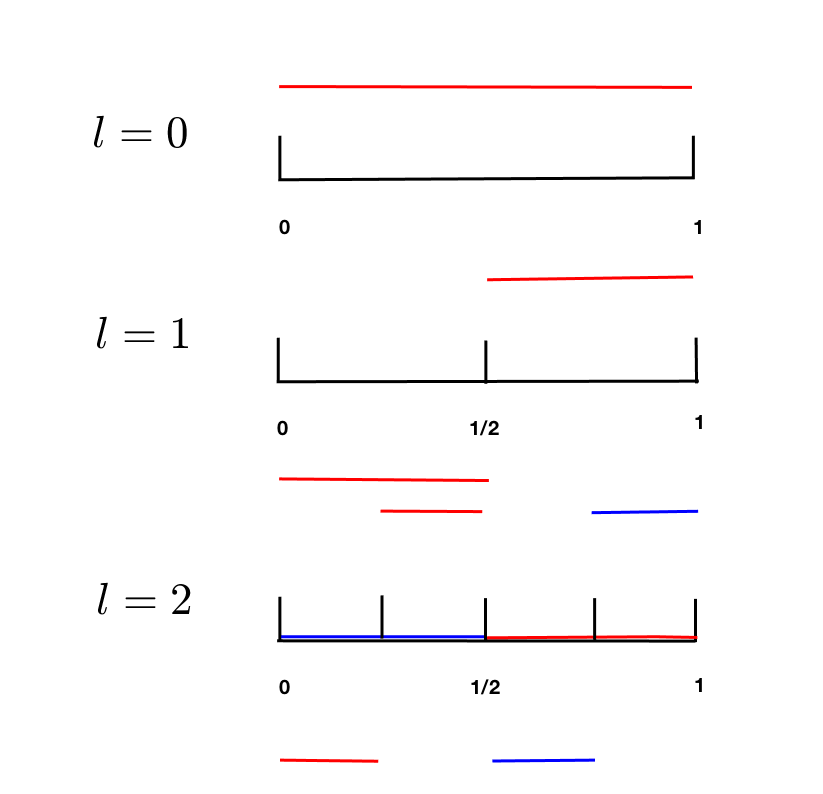
To define the sparse finite element space, we first review the hierarchical decomposition of piecewise polynomial space in one dimension [33]. Consider a general interval , we define the -th level mesh to be a uniform partition of cells with length and , for any Let
be the usual piecewise polynomials of degree at most on . Then, we have the nested structure
Similar to [33], we can now define the multiwavelet subspace , as the orthogonal complement of in with respect to the inner product on , i.e.,
For notational convenience, we let , which is the standard piecewise polynomial space of degree on . This gives the hierarchical decomposition on as .
For a dimensional domain we recall some basic notations about multi-indices. For a multi-index , where denotes the set of nonnegative integers, the and norms are defined as
The component-wise arithmetic operations and relational operations are defined as
By making use of the multi-index notation, we denote by the mesh level in a multivariate sense. We define the tensor-product mesh grid and the corresponding mesh size Based on the grid , we denote by as an elementary cell, and
as the standard tensor-product piecewise polynomial space on this mesh, where denotes the collection of polynomials of degree up to in each dimension on cell . If , the grid and space will be further denoted by and , respectively.
Based on a tensor-product construction, the multi-dimensional increment space can be defined as
Therefore, we have The sparse finite element approximation space we consider, is defined by
This is a subset of , and its number of degrees of freedom scales as [33], which is significantly less than that of with exponential dependence on . This is the key to computational savings in high dimensions.
The standard CDG schemes [18, 20] is characterized by numerical approximations on two sets of overlapping grids: primal and dual meshes. Now, we are ready to incorporate the sparse finite element space defined above into the CDG framework. For the domain under consideration we let be the primal mesh and , which is the periodic extension of restricted to , be the dual mesh. Similarly, we let and to be the periodic extension of restricted to . Here and below, the subscripts and represent the quantities defined on the primal and dual mesh, respectively.
The approximation properties for the sparse finite element space have been established in previous work [33, 12]. By using a lemma in [12], we can have estimates for projection operator onto the spaces
To facilitate the discussion, below we introduce some notations about norms and semi-norms. Let , on primal or dual mesh , we use to denote the standard broken Sobolev norm, i.e. where is the standard Sobolev norm on (and is used to denote the norm). Similarly, we use to denote the broken Sobolev semi-norm, and to denote the broken Sobolev norm and semi-norm that are supported on a general grid . For any set , we define to be the complement set of in For a non-negative integer and set , we define the semi-norm on any domain denoted by
and
which is the norm for the mixed derivative of of at most degree in each direction. In this paper, we use the notation to represent , where the constant is independent of and the mesh level considered. The following results are obtained from Lemma 3.2 in [12].
Lemma 2.1 ( projection estimate).
Let be projections onto the spaces , respectively, then for , , and which is periodic on , , , we have for
| (3) |
This lemma shows that the norm and semi-norm of the projection error scale like and with respect to when the function has bounded mixed derivatives up to enough degrees. This lemma will be used in Theorem 3.2 to establish convergence of the scheme.
Now, we are ready to formulate the sparse grid CDG scheme. Below we review some standard notations about jumps and averages of piecewise functions. With or , let be the collection of all elementary cell , be the union of the interfaces for all the elements in (here we have taken into account the periodic boundary condition when defining ) and be the set of functions defined on . For any and , we define their averages and jumps on the interior edges as follows. Suppose is an interior edge shared by elements and , either on primal or dual mesh, we define the unit normal vectors and on pointing exterior of and , respectively, then
2.2 Discussions on implementations
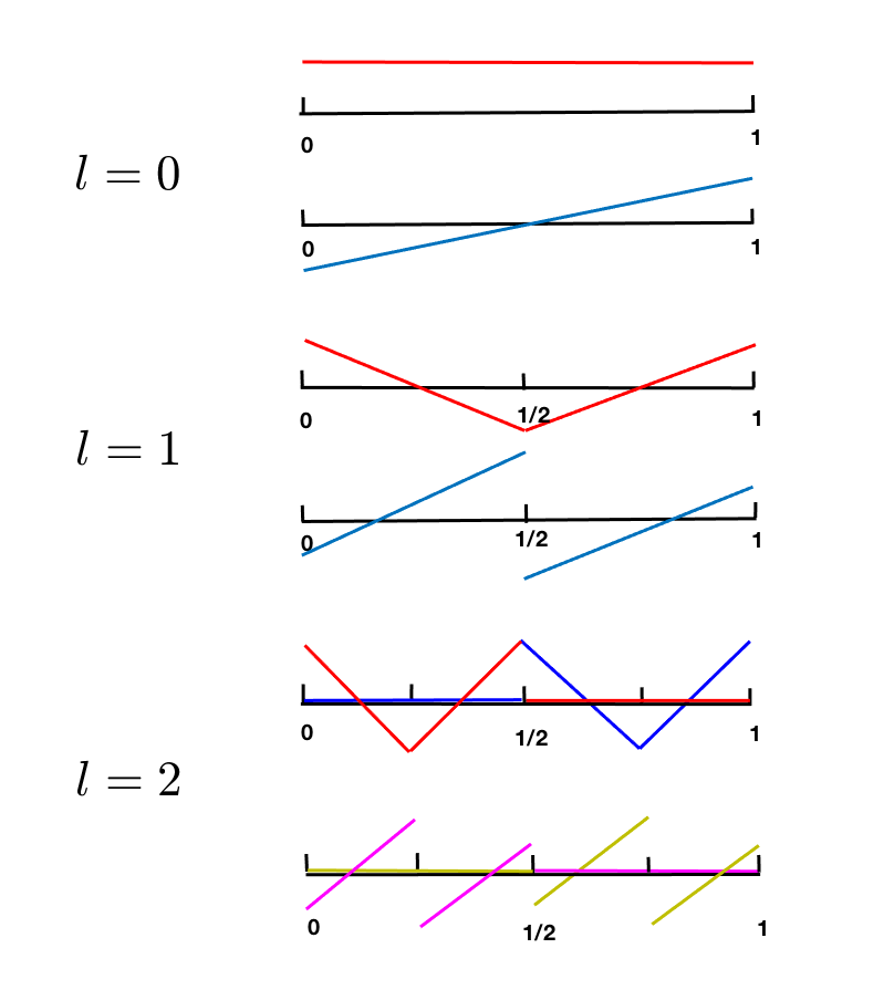
Here, we briefly discuss some details about the implementation of the scheme. We perform the computation by using orthonormal multiwavelet bases constructed by Alpert [1]. In 1D, the bases of are denoted by
and they satisfy . Figures 1(a) and 2(a) provide illustrations of the basis functions for and The bases in in multi-dimensions are defined by tensor products
where we have used the notation and to denote the multi-index for the bases.
As for temporal schemes, we can use the total variation diminishing Runge-Kutta (TVD-RK) methods [32] to solve the ordinary differential equations for the coefficients resulting from the discretization. To calculate the right-hand-side of (4)-(5), the fast matrix-vector product by LU split or LU decomposition algorithms [30, 31, 27] can be applied, by which one can decompose all calculations into one dimensional operations. Below, we briefly describe the LU decomposition algorithm for the calculation of the following matrix-vector product which appears at the right-hand-side of (4)-(5)
where can be the coefficient of the basis in sparse grid space and are the corresponding one-dimensional transform of coefficients from basis to basis in the -th dimension in our scheme. Note that we have one-dimensional bases in each dimension, and we use to denote the -th basis. The bases are ordered according to grid increment. Using Algorithm 1 in [31], we should calculate all the one-dimensional transform along each direction associated with a block lower triangular matrix, and then calculate all the one-dimensional transforms having a block upper triangular structure. The fast matrix-vector product on sparse grid with LU decomposition can be proceeded as follows.
-
1.
Calculate (block) LU decomposition for where are the permutation matrices, are lower and upper triangular matrices.
-
2.
Compute the transform with a (block) lower triangular matrix for
-
3.
Compute the transform with a (block) upper triangular matrix for
Note that in step 1, the LU decomposition pivots only from rows or columns in the same mesh level to maintain the hierarchical structure. This pivoting can be successfully done in the sparse grid CDG scheme, but not in the sparse grid DG scheme, for which additional splitting of the flux terms are deemed necessary for variable coefficient case.
For the integrals involving variable-coefficient, we use Gaussian quadrature to compute these terms. Since these integrals are multi-dimensional integrations, we use the so-called unidirectional principle to separate the integration into multiplication of one-dimensional integrals. For example, if is separable,
When the variable coefficient is separable, we can use unidirectional principle directly. If it is not separable, we can find as the projection of onto the sparse grid finite element space, and then use to compute the integrals.
2.3 Discussions on CFL conditions
It is well known that the CDG schemes allow larger CFL numbers than the standard DG methods except for piecewise constant approximations [20, 26]. Here, we perform a numerical study of the CFL conditions of DG [5], CDG [21], sparse grid DG [12], and the sparse grid CDG schemes. We only consider the two-dimensional case solving constant coefficient equation for now. The results are listed in Table 1. The CFL number of DG method is obtained from Table 2.2 in [5]. The rest of the table is computed by eigenvalue analysis of the discretization matrix, and by requiring the amplification of the eigenvalues to be bounded by 1 in magnitude. We observe that the sparse grid DG method has CFL number that is about two times the CFL number of the standard DG method. The sparse grid CDG method offers the largest CFL conditions among all four methods. Here, as a side note, we find that the CFL number for two-dimensional CDG method is larger than the CFL number for one-dimensional CDG method in [21]. This table shows that one advantage of the sparse grid CDG method is the ability to take large time steps for time evolution problems. In general, further numerical results suggest that for equation the CFL number for sparse grid DG and sparse grid CDG method will change with the value of the coefficients Results in higher dimensions are yet to be studied. A preliminary calculation shows that for equation the CFL conditions for CDG, sparse grid DG and sparse grid CDG methods in 3D are all higher than those for the 2D case in Table 1. The sparse grid CDG method still possesses the largest CFL number among all four methods. Those interesting issues will be investigated in our future work.
| DG | CDG | sparse grid DG | sparse grid CDG | |||||||||
|---|---|---|---|---|---|---|---|---|---|---|---|---|
| 1 | 2 | 3 | 1 | 2 | 3 | 1 | 2 | 3 | 1 | 2 | 3 | |
| 0.33 | – | – | 0.48 | – | – | 0.66 | – | – | 0.87 | – | – | |
| 0.40 | 0.20 | 0.13 | 0.66 | 0.36 | 0.24 | 0.81 | 0.41 | 0.25 | 1.17 | 0.65 | 0.44 | |
| 0.46 | 0.23 | 0.14 | 0.90 | 0.52 | 0.35 | 0.92 | 0.46 | 0.28 | 1.58 | 0.94 | 0.62 | |
2.4 Non-periodic problems
Here, we consider non-periodic problems, where equation (1) or (2) is supplemented by Dirichlet boundary condition on the inflow edges. In this case, we can no longer use periodicity to define the finite element space on the dual mesh, and a new grid hierarchy needs to be introduced.
Recall that for standard CDG methods with non-periodic boundary condition on the domain the finite element space on dual mesh with cell size is represented by
| (6) |
where the mesh is partitioned as
which consists of cells of size and two cells at the left and right ends of size It is easy to see that this space does not have nested structures, i.e. Therefore, we need a new hierarchy to define the increment polynomial spaces.
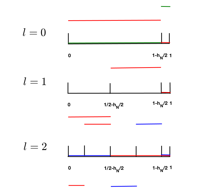
For a fixed refined mesh level we define the following grid on level by a collection of cells as
which consists of cells of size and a cell at the left end of size and a cell at the right end of size This grid structure is naturally nested, and therefore which consists of piecewise polynomials of degree defined on are also nested, and as defined in (6).
Then the definitions of sparse finite element space in Section 2.1 can be naturally extended here. We let , be a complement set of in i.e.
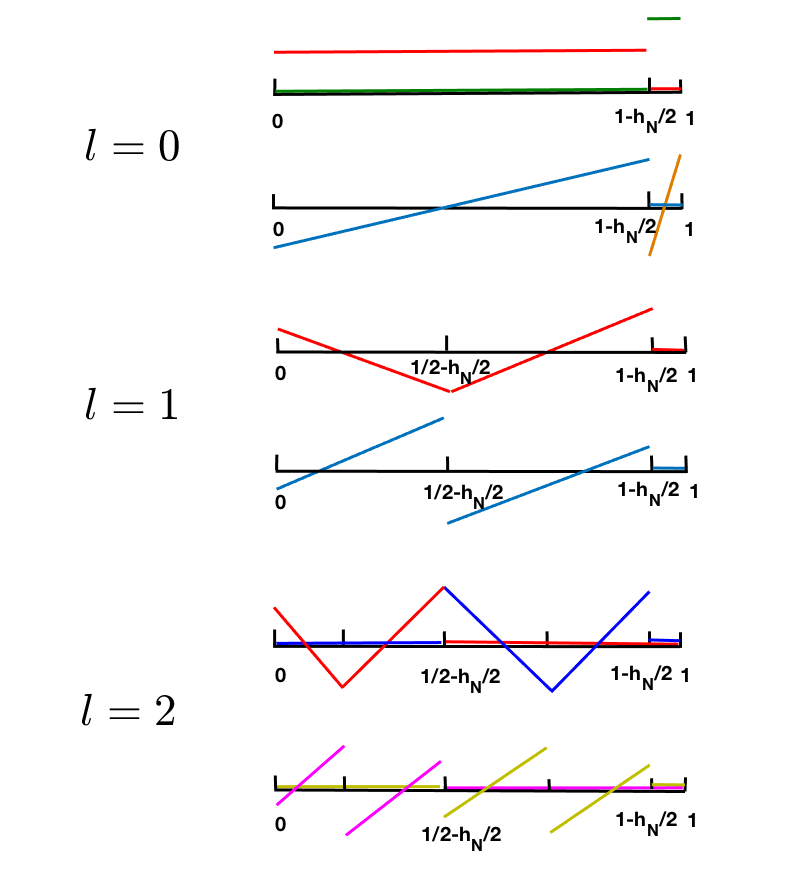
However, we no longer require to be orthogonal to , because such definition will be difficult to implement in practice. Instead, we define to be a span of basis functions that are shifted basis functions of space defined in Section 2.1, namely,
By denoting we have decomposed Illustration of basis functions by such definitions for and can be found in Figures 1(b) and 2(b). The dimension of is while the dimensions of are
Finally, the sparse finite element space on the dual mesh of domain is defined as
where This is a subset of the full grid space , and its number of degrees of freedom scales as (the proof is similar to Lemma 2.3 in [33]), which is larger than that of , but still significantly less than that of with exponential dependence on .
We will now investigate the approximation property of the space We can obtain the following result, which essentially states that the projection onto this newly constructed space has the same order of accuracy as in Lemma 2.1.
Lemma 2.2 ( projection estimate onto ).
Let be the projection onto the space , then for , , and , , , we have
| (7) |
Proof.
The proof follows same procedure as Appendix A in [12]. We will mainly highlight the difference in the proof (see Steps 1 and 2 below). The main difference lies in the fact that all the hierarchical spaces (and associated projections) have dependence not only on but also on the finest mesh level
Step 1: Decomposition of into tensor products of one-dimensional increment projections. We denote as the standard projection operator from to , and the induced increment projection
and further denote
where the last subindex of indicates that the increment operator is defined in -direction. We can verify that In fact, for any , it’s clear that . Therefore, we only need
| (8) |
It suffices to show (8) for which is a dense subset of . In fact, we have
where is the projection onto the full grid space Therefore,
The last term in the first row of the equality above vanishes because In addition, for any ,
Therefore, by properties of the tensor product projections
and the proof for is complete.
Step 2: Estimation of the increment projections. For a function , we have the convergence property of the projection as follows: for any integer with , ,
where the mesh size
The estimation above directly applies for . For , by simple algebra, we have
with .
The rest of the proof is then very similar to Appendix A in [12], and is omitted. ∎
We now provide a numerical validation of Lemma 2.2 by considering the error of projection for a smooth function
| (9) |
In Table 2, we report the errors and the associated orders of accuracy for It is clear that the predicted order of accuracy is achieved.
| error | order | error | order | error | order | ||
| 3 | 8.93E-04 | – | 9.14E-06 | – | 6.40E-08 | – | |
| 4 | 2.61E-04 | 1.77 | 1.29E-06 | 2.82 | 4.45E-09 | 3.85 | |
| 5 | 7.34E-05 | 1.83 | 1.77E-07 | 2.87 | 3.01E-10 | 3.89 | |
| 6 | 2.00E-05 | 1.88 | 2.37E-08 | 2.90 | 1.98E-11 | 3.93 | |
| 7 | 5.35E-06 | 1.90 | 3.11E-09 | 2.93 | 1.29E-12 | 3.94 | |
| 3 | 6.19E-04 | – | 4.93E-06 | – | 3.18E-08 | – | |
| 4 | 1.90E-04 | 1.70 | 7.45E-07 | 2.73 | 2.36E-09 | 3.75 | |
| 5 | 5.71E-05 | 1.73 | 1.10E-07 | 2.76 | 1.69E-10 | 3.80 | |
| 6 | 1.67E-05 | 1.77 | 1.58E-08 | 2.80 | 1.18E-11 | 3.84 | |
| 7 | 4.80E-06 | 1.80 | 2.24E-09 | 2.82 | 9.35E-13 | 3.66 | |
With the aid of this space, the semi-discrete scheme can now be defined similarly as in (4)-(5) by using the space on the dual mesh as and replacing the numerical values on the boundary of the domain by corresponding functions in the Dirichlet boundary conditions.
We now comment on the implementation of this algorithm. As can be seen from Figures 1(b) and 2(b), there are two types of basis functions in 1D for the dual space.
-
•
Type 1 bases (for ), which are the shifted and truncated multiwavelet bases.
-
•
Type 2 bases (for ), which are the Legendre polynomials of degree up to on .
Clearly, Type 1 bases are orthogonal to Type 2 bases, because their support do not overlap. Type 2 bases are orthogonal to each other due to the definition of Legendre polynomials. However, Type 1 bases are no longer orthogonal to each other, due to the domain shift and truncation. However, only the left-most element on each level are changed. For other bases in that level, they will still retain orthogonality. The bases on left-most element in all level are orthogonal to other bases, but not to each other, i.e., the bases defined on left-most element in different levels are not orthogonal. This implies that although the mass matrix is not identity here, it will have block structures and be sparse.
3 Stability and convergence
In this section, we prove stability and error estimates for the sparse grid CDG scheme for the scalar equation. We consider both periodic and non-periodic boundary conditions. For periodic problems, (2) reduces to
| (10) |
where and We assume to avoid the discussion of different boundary conditions for degenerating coefficients. However, there is no difficulty to extend the proof below to degenerating case. For non-periodic problems, the following inflow boundary conditions are prescribed,
where
Correspondingly, we denote the outflow edges by
The scheme for periodic case reduces to: to find and , such that
| (11) | ||||
| (12) |
for any and For non-periodic problems, we require and enforce on the boundary interface.
We can prove that the schemes retain similar stability properties as the standard CDG schemes.
Theorem 3.1 ( Stability).
With periodic boundary condition, the numerical solutions and of the sparse grid CDG scheme (11)-(12) for the equation (10) satisfy the following stability condition
| (13) |
For non-periodic boundary condition, the corresponding numerical solutions satisfy
| (14) |
if
Proof.
Apply divergence theorem, and by periodicity, we have
By the simple inequality ,
and the proof for the periodic case is complete by using Gronwall’s inequality.
For non-periodic boundary condition, we follow the same lines and plug in the corresponding boundary condition,
by noticing and
Let denote the cells on dual mesh adjacent to the boundary in the -th direction. By inverse inequality, we have Therefore,
and the proof for the non-periodic case is complete by using Gronwall’s inequality. ∎
Now we are ready to prove error estimate of the sparse grid CDG scheme.
Theorem 3.2 ( error estimate).
Proof.
For periodic problems, we first introduce the standard notation of bilinear form
By Galerkin orthogonality, we have the error equation
| (16) |
From Theorem 3.1, we get
| (18) |
We write the bilinear form on the right-hand side as a sum of three terms
| (19) |
where
By Cauchy-Schwartz inequality, Lemma 2.1 and , we have
| (20) |
To estimate , we use the following inverse inequalities for ,
and trace inequality,
Then we have
| (21) |
and
| (22) |
Together with the estimates for initial discretization and by Gronwall’s inequality, the proof is complete. For non-periodic problems, the argument is very similar as long as the stability result holds. The proof is omitted for brevity. ∎
This theorem proves error of the scheme is or when the exact solution has enough smoothness in the mixed derivative norms.
4 Numerical results
In this section, we present several numerical tests to validate the performance of the proposed sparse grid CDG schemes. Unless otherwise stated, we use the third-order TVD-RK temporal discretization [32] and choose the time step with for , where is the maximum wave propagation speed in -direction. To guarantee that the spatial error dominates for , we take is taken as which is always smaller than the maximum time step allowed based on the CFL number in Table 1. For periodic problems, we only provide errors on the primal mesh, because the results on the dual mesh are similar. For non-periodic problems, the errors are the average of the errors on the primal and dual meshes.
4.1 Scalar case
In this subsection, we consider the scalar case, i.e.
Example 4.1 (Linear advection with constant coefficients).
We consider
| (23) |
with periodic or Dirichlet boundary conditions on the inflow edges corresponding to the given exact solution.
The exact solution is a smooth function,
In the simulation, we compute the numerical solutions up to two periods in time, meaning that we let final time for , for , and for .
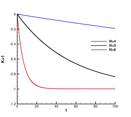
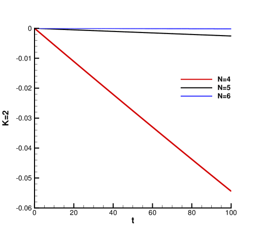
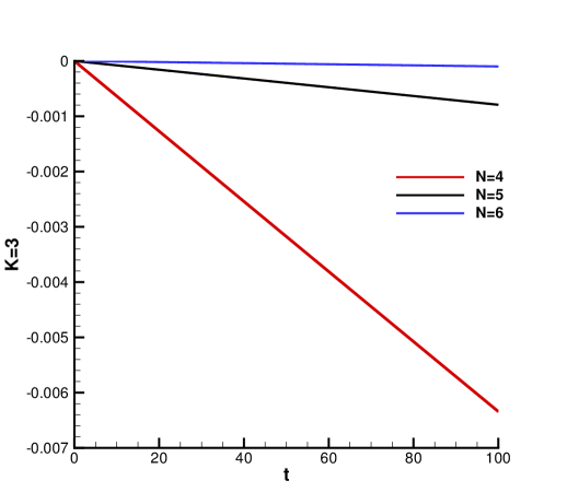
We first test the scheme with periodic boundary condition. In Table 3, we report the errors and orders of accuracy for and up to dimension four. As for accuracy, we observe about half order reduction from the optimal -th order for high-dimensional computations (). The order is slightly better for lower dimensions. The convergence order is similar to the performance of the sparse grid DG scheme in [12]. In Figure 3, we plot the time evolution of the error of norm of numerical solutions and , which is given by
for two-dimensional case for to . From Theorem 3.1, such errors are proportional to the difference between and We can clearly see that the higher order accurate scheme performs way better in conservation of norm due to its higher order accuracy.
| error | order | error | order | error | order | ||
| 3 | 3.14E-01 | – | 1.20E-02 | – | 5.84E-04 | – | |
| 4 | 6.99E-02 | 2.17 | 2.23E-03 | 2.43 | 8.50E-05 | 2.78 | |
| 5 | 1.34E-02 | 2.38 | 4.87E-04 | 2.20 | 3.84E-06 | 4.47 | |
| 6 | 3.43E-03 | 1.97 | 5.97E-05 | 3.03 | 3.89E-07 | 3.30 | |
| 7 | 9.21E-04 | 1.90 | 9.33E-06 | 2.68 | 1.80E-08 | 4.43 | |
| 3 | 6.77E-01 | – | 5.27E-02 | – | 2.13E-03 | – | |
| 4 | 3.56E-01 | 0.93 | 1.10E-02 | 2.26 | 2.62E-04 | 3.02 | |
| 5 | 1.05E-01 | 1.76 | 1.82E-03 | 2.60 | 2.85E-05 | 3.20 | |
| 6 | 2.54E-02 | 2.05 | 5.22E-04 | 1.80 | 2.01E-06 | 3.83 | |
| 7 | 7.45E-03 | 1.77 | 6.89E-05 | 2.92 | 2.01E-07 | 3.32 | |
| 3 | 7.13E-01 | – | 1.26E-01 | – | 4.41E-03 | – | |
| 4 | 6.48E-01 | 0.14 | 3.39E-02 | 1.89 | 7.56E-04 | 2.54 | |
| 5 | 3.80E-01 | 0.77 | 6.91E-03 | 2.29 | 9.82E-05 | 2.94 | |
| 6 | 1.37E-01 | 1.47 | 1.39E-03 | 2.31 | 9.44E-06 | 3.38 | |
| 7 | 3.81E-02 | 1.85 | 3.56E-04 | 1.97 | 8.16E-07 | 3.53 | |
Then, we test the scheme with Dirichlet boundary condition prescribed at the inflow edge according to the exact solution. The results are listed in Table 4. The accuracy order is similar to the periodic case.
| error | order | error | order | error | order | ||
| 3 | 2.66E-01 | – | 1.66E-02 | – | 8.21E-04 | – | |
| 4 | 7.47E-02 | 1.83 | 3.33E-03 | 2.32 | 8.80E-05 | 3.22 | |
| 5 | 1.94E-02 | 1.95 | 5.97E-04 | 2.48 | 4.79E-06 | 4.20 | |
| 6 | 5.44E-03 | 1.83 | 8.60E-05 | 2.80 | 4.50E-07 | 3.41 | |
| 7 | 1.49E-03 | 1.87 | 1.35E-05 | 2.67 | 2.20E-08 | 4.35 | |
| 3 | 6.15E-01 | – | 5.34E-02 | – | 2.67E-03 | – | |
| 4 | 2.86E-01 | 1.10 | 1.40E-02 | 1.93 | 2.87E-04 | 3.22 | |
| 5 | 1.14E-01 | 1.33 | 2.57E-03 | 2.45 | 3.21E-05 | 3.16 | |
| 6 | 3.23E-02 | 1.82 | 5.82E-04 | 2.14 | 2.60E-06 | 3.63 | |
| 7 | 1.03E-02 | 1.65 | 9.81E-05 | 2.57 | 2.86E-07 | 3.18 | |
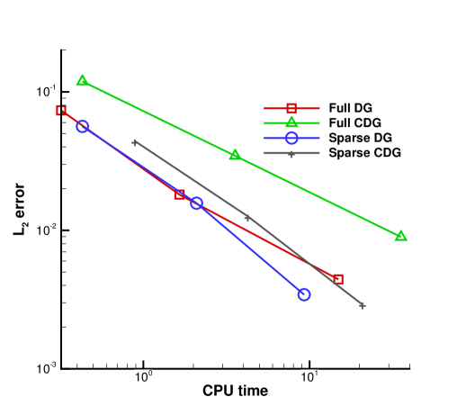
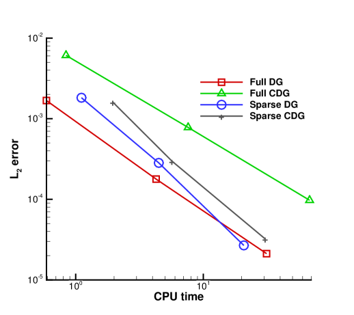
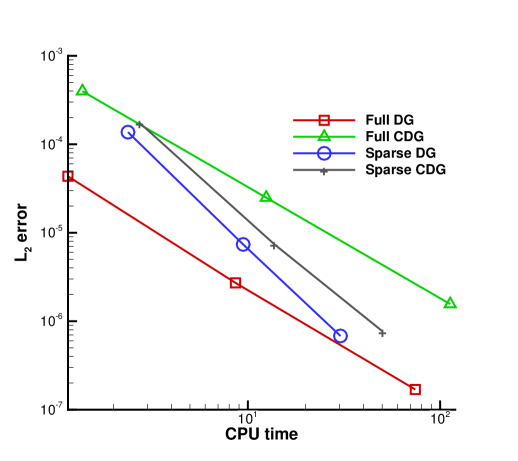
Finally, we use this example to compare the performance of the DG, CDG, sparse grid DG and sparse grid CDG methods. We use the following non-separable initial condition
| (24) |
where When , Runge-Kutta methods of order , respectively, are used for time discretization. We take the time step according to the CFL numbers listed in Table 1. We plot the comparison of the methods measuring errors vs. CPU times in Figure 4. The computations in this example are implemented by an OpenMP code using computational resources from the Institute for Cyber-Enabled Research in Michigan State University. We can see that the sparse grid CDG method outperforms the CDG method, and the sparse grid DG method outperforms the DG method particularly when the mesh level is more refined. When the mesh level increases from to , the CPU cost for sparse grid method grows with the rate of about 4 to 5, while the factor is about 8 to 10 for full grid calculations, respectively, for this 2D case. This shows the advantage of the sparse grid approach. When comparing the sparse grid CDG method with the sparse grid DG method, it seems that for this example, the sparse grid DG method is more efficient. It will be interesting to compare the results for fully nonlinear problems in higher dimensions, for which the CDG method is more advantageous, and this is currently under investigation.
Example 4.2 (Solid body rotation).
We consider solid-body-rotation problems, which are in the form of (1) with
subject to periodic boundary conditions.
Such benchmark tests are commonly used in the literature to assess performance of transport schemes. Here, the initial profile traverses along circular trajectories centered at for and about the axis for without deformation, and it goes back to the initial state after in time. The initial conditions are set to be the following smooth cosine bells (with smoothness),
| (25) |
where when and when , and denotes the distance between and the center of the cosine bell with for and for .
In Table 5, we summarize the convergence study of the numerical solutions computed by the sparse CDG method, including the errors and orders of accuracy. For this variable coefficients equation, we observe at least -th order convergence for all cases. The order is slightly lower than the corresponding ones in Example 4.1.
| error | order | error | order | error | order | ||
| 5 | 1.53E-02 | – | 5.81E-03 | – | 1.34E-03 | – | |
| 6 | 1.02E-02 | 0.58 | 1.50E-03 | 1.95 | 9.64E-05 | 3.80 | |
| 7 | 4.66E-03 | 1.13 | 1.46E-04 | 3.36 | 1.16E-05 | 3.05 | |
| 8 | 1.42E-03 | 1.71 | 2.34E-05 | 2.64 | 1.10E-06 | 3.40 | |
| 5 | 4.83E-03 | – | 6.25E-04 | – | 7.35E-05 | – | |
| 6 | 1.87E-03 | 1.37 | 1.20E-04 | 2.38 | 9.18E-06 | 3.00 | |
| 7 | 7.46E-04 | 1.33 | 3.39E-05 | 1.82 | 1.36E-06 | 2.75 | |
| 8 | 2.55E-04 | 1.55 | 8.11E-06 | 2.06 | 1.94E-07 | 2.81 | |
Example 4.3 (Deformational flow).
We consider the two-dimensional deformational flow with velocity field
where with with periodic boundary condition.
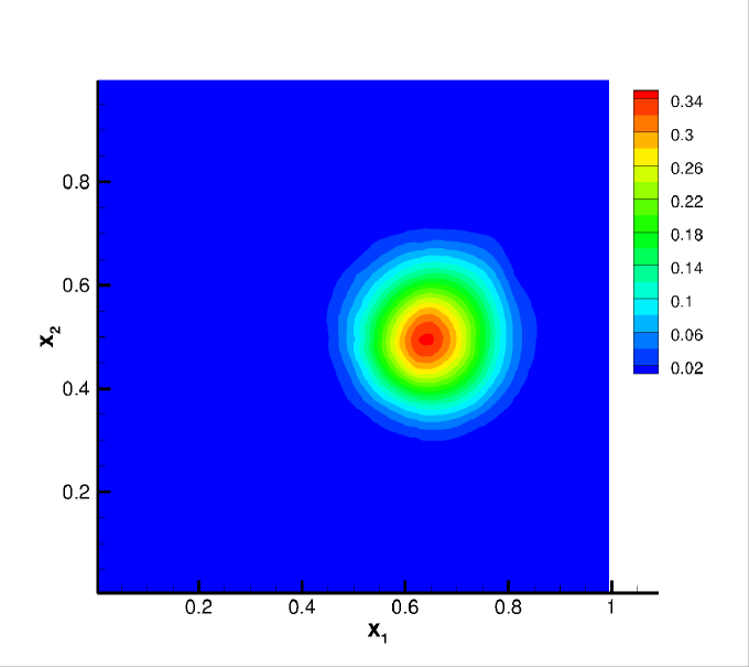
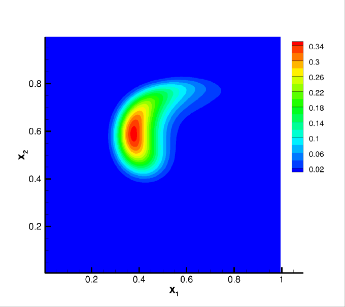
We still adopt the cosine bell (25) as the initial condition for this test, but with and . Note that the deformational test is more challenging than the solid body rotation due to the space and time dependent flow field. In particular, along the direction of the flow, the cosine bell deforms into a crescent shape at , then goes back to its initial state at as the flow reverses. In the simulations, we compute the solution up to . The convergence study is summarized in Table 6. Similar orders are observed compared with Example 4.2. In Figure 5, we plot the contour plots of the numerical solutions on the primal mesh at when the shape of the bell is greatly deformed, and when the solution is recovered into its initial state. It is observed that the sparse CDG scheme with higher degree can better resolve the highly deformed solution structure.
| error | order | error | order | error | order | ||
|---|---|---|---|---|---|---|---|
| 5 | 1/32 | 1.73E-02 | – | 4.37E-03 | – | 1.14E-03 | – |
| 6 | 1/64 | 8.06E-03 | 1.10 | 1.17E-03 | 1.90 | 2.44E-04 | 2.22 |
| 7 | 1/128 | 3.29E-03 | 1.29 | 2.04E-04 | 2.52 | 2.05E-05 | 3.57 |
| 8 | 1/256 | 1.08E-03 | 1.61 | 2.78E-05 | 2.88 | 2.75E-06 | 2.90 |


4.2 System case
Example 4.4 (Acoustic wave equation with constant wave speed).
We consider
| (26) |
with periodic boundary conditions. The initial conditions and are chosen according to the following two types of exact solutions: the standing wave
and the traveling wave
We compute the solution until Similar to the scalar case, we present the errors and orders of accuracy for in Table 7. From the table, we still observe at least -th order for the solution.
| error | order | error | order | error | order | ||
|---|---|---|---|---|---|---|---|
| standing wave | |||||||
| 3 | 3.56E-01 | – | 1.05E-02 | – | 5.37E-04 | – | |
| 4 | 7.93E-02 | 2.17 | 1.84E-03 | 2.51 | 4.31E-05 | 3.64 | |
| 5 | 1.50E-02 | 2.40 | 3.18E-04 | 2.53 | 3.39E-06 | 3.67 | |
| 6 | 3.72E-03 | 2.01 | 4.95E-05 | 2.68 | 2.77E-07 | 3.61 | |
| 7 | 1.01E-03 | 1.88 | 7.60E-06 | 2.70 | 2.03E-08 | 3.77 | |
| traveling wave | |||||||
| 3 | 3.97E-01 | – | 1.85E-02 | – | 7.75E-04 | – | |
| 4 | 8.58E-02 | 2.21 | 3.36E-03 | 2.46 | 6.76E-05 | 3.52 | |
| 5 | 1.97E-02 | 2.12 | 6.07E-04 | 2.47 | 5.68E-06 | 3.57 | |
| 6 | 5.36E-03 | 1.88 | 9.66E-05 | 2.65 | 4.44E-07 | 3.68 | |
| 7 | 1.50E-03 | 1.84 | 1.45E-05 | 2.74 | 3.39E-08 | 3.71 | |
Example 4.5 (Two-dimensional homogeneous isotropic elastic wave [15]).
The 2D elastic wave equation in homogeneous and isotropic medium in velocity-stress formulation without external source, is a linear hyperbolic system of the form
| (27) |
where , represents the normal stress and represents the shear stress and are the velocity in and directions.
where and are the Lamé constants and is the mass density of material. Eigenvalues of and are , which give us the wave speed and for P-wave and S-wave respectively. We consider the homogeneous material parameters , then . On domain , we take the solutions consisting of a plane P-wave traveling along diagonal direction and a plane S-wave traveling in the opposite direction, i.e.,
where and . Periodic boundary condition is applied and the initial condition is chosen as .
We compute the solution until The errors and orders of accuracy for are shown in Table 8. We observe that the convergence order is close to .
| error | order | error | order | error | order | ||
|---|---|---|---|---|---|---|---|
| 4 | 1.09E+00 | – | 2.72E-01 | – | 5.71E-02 | – | |
| 5 | 7.47E-01 | 0.55 | 6.48E-02 | 2.07 | 6.19E-03 | 3.21 | |
| 6 | 2.41E-01 | 1.63 | 9.65E-03 | 2.75 | 4.77E-04 | 3.70 | |
| 7 | 7.14E-02 | 1.76 | 1.12E-03 | 3.11 | 2.55E-05 | 4.23 | |
Example 4.6 (Three-dimensional isotropic elastic wave [6]).
We extend the previous example to 3D and obtain the following linear hyperbolic system
| (28) |
where , is the stress tensor and are the velocities in each spatial direction.
where and take the same values as the previous example. Hence, we have the same values for and . Eigenvalues of and are , which describe the wave speed for P-wave and S-wave (with different polarizations). On domain , we take the solutions consisting of a plane S-wave traveling along diagonal direction and a plane P-wave traveling in the opposite direction, i.e.,
where
and . Similarly, we consider periodic boundary condition and as initial condition.
We present the numerical results at In Table 9, we get at least -th order of accuracy for the solution .
| error | order | error | order | error | order | ||
|---|---|---|---|---|---|---|---|
| 4 | 2.49E+00 | – | 4.93E-02 | – | 8.91E-04 | – | |
| 5 | 7.70E-01 | 1.69 | 8.17E-03 | 2.59 | 8.66E-05 | 3.36 | |
| 6 | 1.76E-01 | 2.13 | 1.59E-03 | 2.36 | 7.12E-06 | 3.60 | |
| 7 | 4.27E-02 | 2.04 | 2.79E-04 | 2.51 | 5.42E-07 | 3.72 | |
5 Conclusions and future work
In this work, we develop sparse grid CDG schemes for linear transport problems. We construct sparse finite element space on primal and dual meshes for periodic and non-periodic problems. A new hierarchical representation of the piecewise polynomials is introduced and analyzed for non-periodic problems on the dual mesh. Compared with CDG scheme, the method is shown to be efficient for high dimensional problems. Compared with sparse grid DG scheme, the method proposed allows larger CFL numbers and avoid the evaluations of numerical fluxes. We show that for scalar equation with constant coefficients, the scheme shares similar stability property as the standard CDG scheme. convergence rate is proved to be of where is the most refined mesh in each direction. Numerical results are provided validating performance of the methods. In particular, the convergence order seems higher than the theoretically predicted rate, which suggests that new projection techniques may be needed. Other future work includes detailed study of CFL conditions, and applications and extensions to nonlinear and nonsmooth problems.
References
- [1] B. Alpert. A class of bases in 2 for the sparse representation of integral operators. SIAM J. Math. Anal., 24(1):246–262, 1993.
- [2] R. Bellman. Adaptive control processes: a guided tour, volume 4. Princeton University Press Princeton, 1961.
- [3] H.-J. Bungartz and M. Griebel. Sparse grids. Acta numer., 13:147–269, 2004.
- [4] B. Cockburn, G. Karniadakis, and C.-W. Shu. The development of discontinuous Galerkin methods. In B. Cockburn, G. Karniadakis, and C.-W. Shu, editors, Discontinuous Galerkin methods: theory, computation and applications, volume 11, pages 3–50. Springer, 2000.
- [5] B. Cockburn and C.-W. Shu. Runge-Kutta discontinuous Galerkin methods for convection-dominated problems. J. Sci. Comput., 16:173–261, 2001.
- [6] M. Dumbser and M. Käser. An arbitrary high-order discontinuous Galerkin method for elastic waves on unstructured meshes—II. The three-dimensional isotropic case. Geophys. J. Int., 167(1):319–336, 2006.
- [7] J. Garcke and M. Griebel. Sparse grids and applications. Springer, 2013.
- [8] V. Gradinaru. Fourier transform on sparse grids: code design and the time dependent Schrödinger equation. Computing, 80(1):1–22, 2007.
- [9] M. Griebel. Adaptive sparse grid multilevel methods for elliptic pdes based on finite differences. Computing, 61(2):151–179, 1998.
- [10] M. Griebel and J. Hamaekers. Sparse grids for the Schrödinger equation. ESAIM: Math. Model. Numer. Anal., 41(02):215–247, 2007.
- [11] M. Griebel and G. Zumbusch. Adaptive sparse grids for hyperbolic conservation laws. In Hyperbolic problems: theory, numerics, applications, pages 411–422. Springer, 1999.
- [12] W. Guo and Y. Cheng. A sparse grid discontinuous Galerkin method for high-dimensional transport equations and its application to kinetic simulations. SIAM J. Sci. Comput., 38(6):A3381–A3409, 2016.
- [13] W. Guo and Y. Cheng. An adaptive multiresolution discontinuous Galerkin method for time-dependent transport equations in multidimensions. SIAM J. Sci. Comput., 39(6):A2962–A2992, 2017.
- [14] P. Hemker. Sparse-grid finite-volume multigrid for 3D-problems. Adv. Comput. Math., 4(1):83–110, 1995.
- [15] M. Käser and M. Dumbser. An arbitrary high-order discontinuous Galerkin method for elastic waves on unstructured meshes—I. The two-dimensional isotropic case with external source terms. Geophys. J. Int., 166(2):855–877, 2006.
- [16] A. Kurganov and E. Tadmor. New high-resolution central schemes for nonlinear conservation laws and convection–diffusion equations. J. Comput. Phys., 160(1):241–282, 2000.
- [17] R. J. LeVeque. Finite volume methods for hyperbolic problems, volume 31. Cambridge university press, 2002.
- [18] Y. Liu. Central schemes and central discontinuous Galerkin methods on overlapping cells. 2005.
- [19] Y. Liu. Central schemes on overlapping cells. J. Comput. Phys., 209(1):82–104, 2005.
- [20] Y. Liu, C.-W. Shu, E. Tadmor, and M. Zhang. Central discontinuous Galerkin methods on overlapping cells with a nonoscillatory hierarchical reconstruction. SIAM J. Numer. Anal., 45(6):2442–2467, 2007.
- [21] Y. Liu, C.-W. Shu, E. Tadmor, and M. Zhang. L2 stability analysis of the central discontinuous Galerkin method and a comparison between the central and regular discontinuous Galerkin methods. ESAIM: Math. Model. Numer. Anal., 42(4):593–607, 2008.
- [22] Y. Liu, C.-W. Shu, and M. Zhang. Optimal error estimates of the semidiscrete central discontinuous galerkin methods for linear hyperbolic equations. SIAM J. Numer. Anal., 56(1):520–541, 2018.
- [23] X. Ma and N. Zabaras. An adaptive hierarchical sparse grid collocation algorithm for the solution of stochastic differential equations. J. Comput. Phys., 228(8):3084–3113, 2009.
- [24] H. Nessyahu and E. Tadmor. Non-oscillatory central differencing for hyperbolic conservation laws. J. Comput. Phys., 87(2):408–463, 1990.
- [25] F. Nobile, R. Tempone, and C. Webster. A sparse grid stochastic collocation method for partial differential equations with random input data. SIAM J. Numer. Anal., 46(5):2309–2345, 2008.
- [26] M. A. Reyna and F. Li. Operator bounds and time step conditions for the DG and central DG methods. J. Sci. Comput., 62(2):532–554, 2015.
- [27] Z. Rong, J. Shen, and H. Yu. A nodal sparse grid spectral element method for multi-dimensional elliptic partial differential equations. Int. J. Numer. Anal. Model., 14(4-5):762–783, 2017.
- [28] C. Schwab, E. Süli, and R. Todor. Sparse finite element approximation of high-dimensional transport-dominated diffusion problems. ESAIM: Math. Model. Numer. Anal., 42(05):777–819, 2008.
- [29] J. Shen and L.-L. Wang. Sparse spectral approximations of high-dimensional problems based on hyperbolic cross. SIAM J. Numer. Anal., 48(3):1087–1109, 2010.
- [30] J. Shen and H. Yu. Efficient spectral sparse grid methods and applications to high-dimensional elliptic problems. SIAM J. Sci. Comput., 32(6):3228–3250, 2010.
- [31] J. Shen and H. Yu. Efficient spectral sparse grid methods and applications to high-dimensional elliptic equations II. unbounded domains. SIAM J. Sci. Comput., 34(2):A1141–A1164, 2012.
- [32] C.-W. Shu and S. Osher. Efficient implementation of essentially non-oscillatory shock-capturing schemes. J. Comput. Phys., 77:439–471, 1988.
- [33] Z. Wang, Q. Tang, W. Guo, and Y. Cheng. Sparse grid discontinuous Galerkin methods for high-dimensional elliptic equations. J. Comput. Phys., 314:244—263, 2016.
- [34] D. Xiu. Efficient collocational approach for parametric uncertainty analysis. Comm. Comput. Phys., 2(2):293–309, 2007.
- [35] D. Xiu and J. Hesthaven. High-order collocation methods for differential equations with random inputs. SIAM J. Sci. Comput., 27(3):1118–1139, 2005.
- [36] C. Zenger. Sparse grids. In Parallel Algorithms for Partial Differential Equations, Proceedings of the Sixth GAMM-Seminar, volume 31, 1990.