Sparse group lasso and high dimensional multinomial classification.
Abstract
The sparse group lasso optimization problem is solved using a coordinate gradient descent algorithm. The algorithm is applicable to a broad class of convex loss functions. Convergence of the algorithm is established, and the algorithm is used to investigate the performance of the multinomial sparse group lasso classifier. On three different real data examples the multinomial group lasso clearly outperforms multinomial lasso in terms of achieved classification error rate and in terms of including fewer features for the classification. The run-time of our sparse group lasso implementation is of the same order of magnitude as the multinomial lasso algorithm implemented in the R package glmnet. Our implementation scales well with the problem size. One of the high dimensional examples considered is a 50 class classification problem with 10k features, which amounts to estimating 500k parameters. The implementation is available as the R package msgl.
keywords:
Sparse group lasso , classification , high dimensional data analysis , coordinate gradient descent , penalized loss.1 Introduction
The sparse group lasso is a regularization method that combines the lasso [1] and the group lasso [2]. Friedman et al. [3] proposed a coordinate descent approach for the sparse group lasso optimization problem. Simon et al. [4] used a generalized gradient descent algorithm for the sparse group lasso and considered applications of this method for linear, logistic and Cox regression. We present a sparse group lasso algorithm suitable for high dimensional problems. This algorithm is applicable to a broad class of convex loss functions. In the algorithm we combine three non-differentiable optimization methods: the coordinate gradient descent [5], the block coordinate descent [6] and a modified coordinate descent method.
Our main application is to multinomial regression. In Section 1.1 we introduce the general sparse group lasso optimization problem with a convex loss function. Part I investigates the performance of the multinomial sparse group lasso classifier. In Part II we present the general sparse group lasso algorithm and establish convergence.
The formulation of an efficient and robust sparse group lasso algorithm is not straight forward due to non-differentiability of the penalty. Firstly, the sparse group lasso penalty is not completely separable, which is problematic when using a standard coordinate descent scheme. To obtain a robust algorithm an adjustment is necessary. Our solution is a minor modification of the coordinate descent algorithm; it efficiently treats the singularity at zero that cannot be separated out. Secondly, our algorithm is a Newton type algorithm; hence we sequentially optimize penalized quadratic approximations of the loss function. This approach raises another challenge: how to reduce the costs of computing the Hessian? In Section 4.6 we show that an upper bound on the Hessian is sufficient to determine whether the minimum over a block of coefficients is attained at zero. This approach enables us to update a large percentage of the blocks without computing the complete Hessian. In this way we reduce the run-time, provided that the upper bound of the Hessian can be computed efficiently. We found that this approach reduces the run-time on large data sets by a factor of more than 2.
Our focus is on applications of the multinomial sparse group lasso to problems with many classes. For this purpose we choose three multiclass classification problems. We found that the multinomial group lasso and sparse group lasso perform well on these problems. The error rates were substantially lower than the best obtained with multinomial lasso, and the low error rates were achieved for models with fewer features having non-zero coefficients. For example, we consider a text classification problem consisting of Amazon reviews with 50 classes and 10k textual features. This problem showed a large improvement in the error rates: from approximately 40% for the lasso to less than 20% for the group lasso.
We provide a generic implementation of the sparse group lasso algorithm in the form of a
C++ template library. The implementation for multinomial and logistic sparse group lasso
regression is available as an R package. For our implementation the time to compute the
sparse group lasso solution is of the same order of magnitude as the time required for the
multinomial lasso algorithm as implemented in the R-package glmnet. The computation time
of our implementation scales well with the problem size.
1.1 Sparse group lasso
Consider a convex, bounded below and twice continuously differentiable function . We say that is a sparse group lasso minimizer if it is a solution to the unconstrained convex optimization problem
| (1) |
where is the sparse group lasso penalty (defined below) and .
Before defining the sparse group lasso penalty some notation is needed. We decompose the search space
into blocks having dimensions for , hence . For a vector we write where . For we call the ’th block of . We use the notation to denote the ’th coordinate of the ’th block of , whereas is the ’th coordinate of .
Definition 1 (Sparse group lasso penalty).
The sparse group lasso penalty is defined as
for , group weights , and parameter weights where .
The sparse group lasso penalty includes the lasso penalty () and the group lasso penalty (). Note also that for sufficiently large values of the minimizer of (1) is zero. The infimum of these, denoted , is computable, see Section 4.2.
We emphasize that the sparse group lasso penalty is specified by
-
1.
a grouping of the parameters ,
-
2.
and the weights and .
In Part I we consider multinomial regression; here the parameter grouping is given by the multinomial model. For multinomial as well as other regression models, the grouping can also reflect a grouping of the features.
Part I The multinomial sparse group lasso classifier
In this section we examine the characteristics of the multinomial sparse group lasso method. Our main interest is the application of the multinomial sparse group lasso classifier to problems with many classes. For this purpose we have chosen three classification problems based on three different data sets, with 10, 18 and 50 classes. In [7] the microRNA expression profile of different types of primary cancer samples is studied. In Section 3.1 we consider the problem of classifying the primary site based on the microRNA profiles in this data set. The Amazon reviews author classification problem, presented in [8], is studied in Section 3.2. The messenger RNA profile of different human muscle diseases is studied in [9]. We consider, in Section 3.3, the problem of classifying the disease based on the messenger RNA profiles in this data set. Table 1 summarizes the dimensions and characteristics of the data sets and the associated classification problems. Finally, in Section 4, we examine the characteristics of the method applied to simulated data sets.
2 Setup
Consider a classification problem with classes, samples, and features. Assume given a data set where, for all , is the observed feature vector and is the categorical response. We organize the feature vectors in the design matrix
As in [10] we use a symmetric parametrization of the multinomial model. With given by
the multinomial model is specified by
The model parameters are organized in the -dimensional vector, , of intercept parameters together with the matrix
| (2) |
where are the parameters associated with the ’th feature. The lack of identifiability in this parametrization is in practice dealt with by the penalization.
The log-likelihood is
| (3) |
Our interest is the sparse group lasso penalized maximum likelihood estimator. That is, is estimated as a minimizer of the sparse group lasso penalized negative-log-likelihood:
| (4) |
In our applications we let for all and for all , but other choices are possible in the implementation. Note that the parameter grouping, as part of the penalty specification, is given in terms of the columns in (2), i.e. .
3 Data examples
| Data set | Features | |||
|---|---|---|---|---|
| Cancer sites | microRNA expressions | 18 | 162 | 217 |
| Amazon reviews | Various textual features | 50 | 1500 | 10k |
| Muscle diseases | Gene expression | 10 | 107 | 22k |
The data sets were preprocessed before applying the multinomial sparse group lasso estimator. Two preprocessing schemes were used: normalization and standardization. Normalization entails centering and scaling of the samples in order to obtain a design matrix with row means of 0 and row variance of 1. Standardization involves centering and scaling the features to obtain a design matrix with column means of 0 and column variance of 1. Note that the order in which normalization and standardization are applied matters.
The purpose of normalization is to remove technical (non-biological) variation. A range of different normalization procedures exist for biological data. Sample centering and scaling is one of the simpler procedures. We use this simple normalization procedure for the two biological data sets in this paper. Normalization is done before and independent from the sparse group lasso algorithm.
The purpose of standardization is to create a common scale for features. This ensures that differences in scale will not influence the penalty and thus the variable selection. Standardization is an option for the sparse group lasso implementation, and it is applied as the last preprocessing step for all three example data sets.
We want to compare the performance of the multinomial sparse group lasso estimator for different values of the regularization parameter . Applying the multinomial sparse group lasso estimator with a given and -sequence, , results in a sequence of estimated models with parameters . The generalization error can be estimated by cross validation [11]. For our applications we keep the sample ratio between classes in the cross validation subsets approximately fixed to that of the entire data set. Hence, we may compute a sequence, , of estimated expected generalization errors for the sequence of models. However, for given and we cannot simply compare and , since the value is scaled differently for different values of . We will instead compare the models with the same number of non-zero parameters and the same number of non-zero parameter groups, respectively. Define
with the estimator of for the given values of and . That is, is the number of non-zero parameter blocks in the fitted model. Note that there is a one-to-one correspondence between parameter blocks and features in the design matrix. Furthermore, we define the total number of non-zero parameters as
In particular, we want to compare the fitted models with the same number of parameter blocks. There may, however, be more than one -value corresponding to a given value of . Thus we compare the models on a subsequence of the -sequence. With for denoting the different elements of the set in increasing order we define
We then compare the characteristics of the multinomial sparse group lasso estimators for different values by comparing the estimates
3.1 Cancer sites
The data set consists of bead-based expression data for 217 microRNAs from normal and cancer tissue samples. The samples are divided into 11 normal classes, 16 tumor classes and 8 tumor cell line classes. For the purpose of this study we select the normal and tumor classes with more than 5 samples. This results in an 18 class data set with 162 samples. The data set is unbalanced, with the number of samples in each class ranging from 5 to 26 and with an average of 9 samples per class. Data was normalized and then standardized before running the sparse group lasso algorithm. For more information about this data set see [7]. The data set is available from the Gene Expression Omnibus with accession number GSE2564.
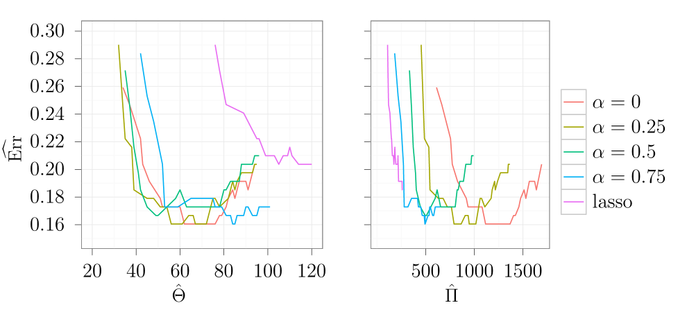
Figure 1 shows the result of a 10-fold cross validation for 5 different values of , including the lasso and group lasso. The -sequence runs from to , with . It is evident that the group lasso and sparse group lasso models achieve a lower expected error using fewer genes than the lasso model. However, models with a low value have a larger number of non-zero parameters than models with a high value. A reasonable compromise could be the model with . This model does not only have a low estimated expected error, but the low error is also achieved with a lower estimated number of non-zero parameters, compared to group lasso.
3.2 Amazon reviews
The Amazon review data set consists of 10k textual features (including lexical, syntactic, idiosyncratic and content features) extracted from 1500 customer reviews from the Amazon Commerce Website. The reviews were collected among the reviews from 50 authors with 50 reviews per author. The primary classification task is to identify the author based on the textual features. The data and feature set were presented in [8] and can be found in the UCI machine learning repository [12]. In [8] a Synergetic Neural Network is used for author classification, and a k feature based 10-fold CV accuracy of 0.805 is reported. The feature selection and training of the classifier were done separately.
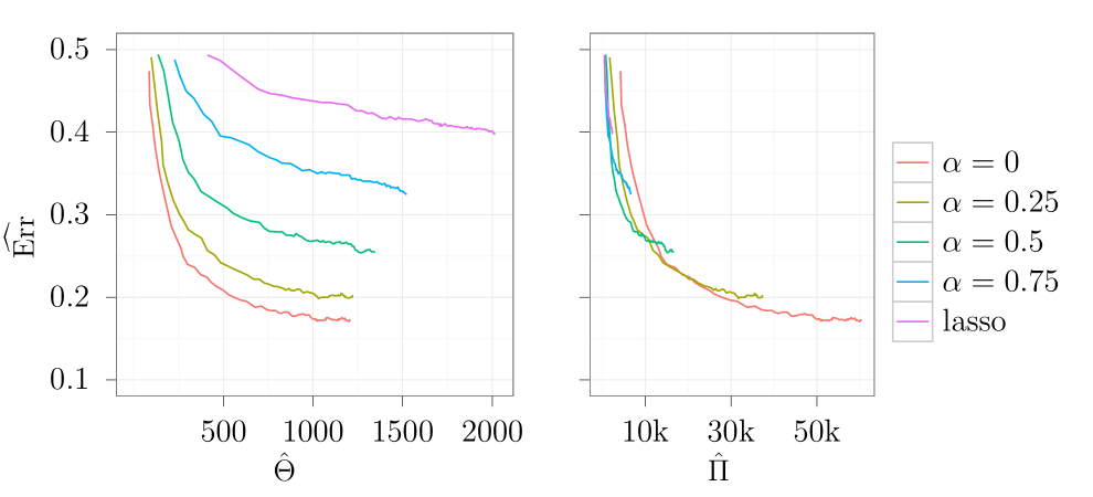
We did 10-fold cross validation using multinomial sparse group lasso for five different values of . The results are shown in Figure 2. The -sequence runs from to , with . The design matrix is sparse for this data set. Our implementation of the multinomial sparse group lasso algorithm utilizes the sparse design matrix to gain speed and for memory efficiency. No normalization was applied for this data set. Features were scaled to have variance 1, but were not centered.
For this data set it is evident that lasso performs badly and that the group lasso performs best - in fact much better than lasso. The group lasso achieves an accuracy of around 0.82 with a feature set of size k. This outperforms the neural network in [8].
3.3 Muscle diseases
This data set consists of messenger RNA array expression data of 119 muscle biopsies from patients with various muscle diseases. The samples are divided into 13 diagnostic groups. For this study we only consider classes with more than 5 samples. This results in a classification problem with 107 samples and 10 classes. The data set is unbalanced with class sizes ranging from 4 to 20 samples per class. Data was normalized and then standardized before running the sparse group lasso algorithm. For background information on this data set, see [9]. The data set is available from the Gene Expression Omnibus with accession number GDS1956.
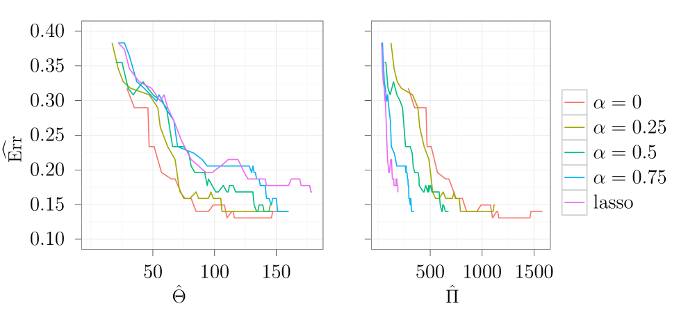
The results of a 10-fold cross validation are shown in Figure 3. The -sequence runs from to , with . We see the same trend as in the other two data examples. Again the group lasso models perform well, however not significantly better than the closest sparse group lasso models (). The lasso models perform reasonably well on this data set, but they are still outperformed by the sparse group lasso models.
4 A simulation study
In this section we investigate the characteristics of the sparse group lasso estimator on simulated data sets. We are primarily interested in trends in the generalization error as is varied and is selected by cross validation on a relatively small training set. We suspect that this trend will depend on the distribution of the data. We restrict our attention to multiclass data where the distribution of the features given the class is Gaussian. Loosely speaking, we suspect that if the differences in the data distributions are very sparse, i.e. the centers of the Gaussian distributions are mostly identical across classes, the lasso will produce models with the lowest generalization error. If the data distribution is sparse, but not very sparse, then the optimal is in the interval . For a dense distribution, typically with differences being among all classes, we expect the group lasso to perform best. The simulation study confirms this.
The mathematical formulation is as follows. Let
where for and . Denote by a data set consisting of samples for each of the classes – each sampled from the Gaussian distribution with centers , respectively, and with a common covariance matrix . Let be the smallest -value with the minimal estimated expected generalization error, as determined by cross validation on . Denote by the generalization error of the model that has been estimated from the training set , by the sparse group lasso, for the given values of and . Then let
where is the Bayes rate. We are interested in trends in , as a function of , for different configurations of . To be specific, we will sample from one of the following distributions:
-
1.
A sparse model distribution, where the first entries of are i.i.d. with a distribution that is a mixture of the uniform distribution on and the degenerate distribution at 0 with point probability .
-
2.
A dense model distribution, where the first entries of are i.i.d. Laplace distributed with location 0 and scale .
The last entries are zero. We take throughout for the sparse model distribution. The within class covariance matrix is constructed using features from the cancer site data set. Let be the empirical covariance matrix of randomly chosen features. To avoid that the covariance matrix become singular we take
for .
The primary quantity of interest is
| (5) |
the expectation being over and the data set . We are also interested in how well we can estimate the non-zero patterns of the ’s. Consider this as two class classification problems, one for each parameter, where we predict the to be non-zero if is non-zero, and to be zero otherwise. We calculate the number of false positives, true positives, false negatives and true negatives. The positive predictive value (ppv) and the true positive rate (tpr) are of particular interest. The true positive rate measures how sensitive a given method is at discovering non-zero entries. The positive predictive value measures the precision with which the method is selecting the non-zero entries. We consider the following two quantities
| (6) |
In order to estimate the quantities (5) and (6) we sample configurations of from one of the above distributions. For each configuration we sample a training and a test data set of sizes and , respectively. Using the training data set we fit the model and estimate using the test data set. Estimates , and are the corresponding averages over the configurations.
For this study we chose , , , , and the following three configuration distributions:
-
1.
Thin configurations, where the centers are distributed according to the sparse model distribution with , as defined above.
-
2.
Sparse configurations, where the centers are distributed according to the sparse model distribution with .
-
3.
Dense configurations, where the centers are distributed according to the dense model distribution with scale and .
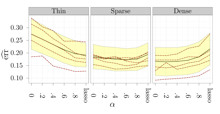
In Figure 4 we see that for thin configurations the lasso has the lowest estimated error gab, along with the sparse group lasso with . For the sparse configurations the results indicate that the optimal choice of is in the open interval , but in this case all choices of result in a comparable error gab. For the dense configurations the group lasso is among the methods with the lowest error gab.
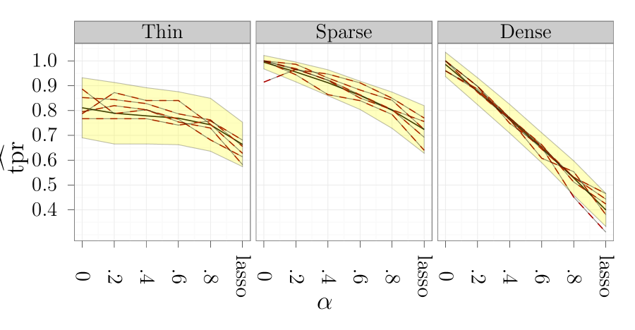
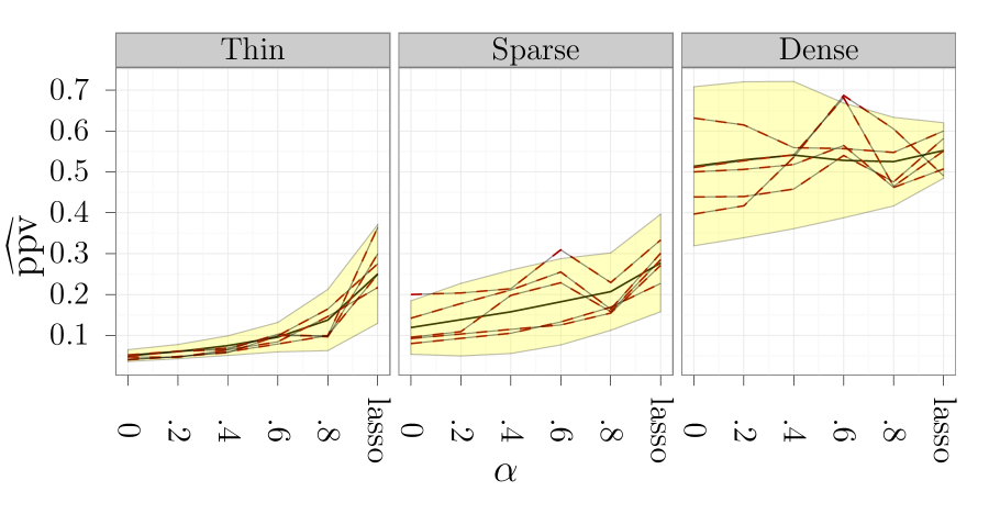
In Figure 5 we plotted the true positive rate for the three configurations. Except for the thin configurations, the lasso is markedly less sensitive than the sparse group and group lasso methods. However, looking at Figure 6 we see that the sparse group and group lasso methods have a lower precision than the lasso, except for the dense configurations. We note that the group lasso has the worst precision, except for the dense configurations.
Part II The sparse group lasso algorithm
In this section we present the sparse group lasso algorithm. The algorithm is applicable to a broad class of loss functions. Specifically, we require that the loss function is convex, twice continuously differentiable and bounded below. Additionally, we require that all quadratic approximations around a point in the sublevel set
are bounded below, where is the initial point. The last requirement will ensure that all subproblems are well defined.
The algorithm solves (1) for a decreasing sequence of values ranging from to a user specified . The algorithm consists of four nested main loops:
In Section 4.3 to 4.5 we discuss the outer, middle and inner loop, respectively. In Section 4.6 we develop a method allowing us to bypass computations of large parts of the Hessian, hereby improving the performance of the middle loop. Section 5 provides a discussion of the available software solutions, as well as run-time performance of the current implementation.
The theoretical basis of the optimization methods we apply can be found in [6, 5]. A short review tailored to this paper is given in A.
4.1 The sparse group lasso penalty
In this section we derive fundamental results regarding the sparse group lasso penalty.
We first observe that is separable in the sense that if, for any group , we define the convex penalty by
then . Separability of the penalty is required to ensure convergence of coordinate descent methods, see [5, 6], and see also A.
In a block coordinate descent scheme the primary minimization problem is solved by minimizing each block, one at a time, until convergence. We consider conditions ensuring that
| (7) |
for a given convex and twice continuously differentiable function . For a straightforward calculation shows that the subgradient of at zero is
where , and where for denotes the diagonal matrix with diagonal . For an introduction to the theory of subgradients see Chapter 4 in [13].
Proposition 1 below gives a necessary and sufficient condition for (7) to hold. Before we state the proposition the following definition is needed.
Definition 2.
For we define the map by
and the function by
Proposition 1.
Assume given , and define the closed sets
Then the following hold:
-
a.
.
-
b.
if and only if .
-
c.
If then .
The following observations will prove to be valuable. Note that we use to denote coordinatewise ordering.
Lemma 1.
For any three vectors the following hold:
-
a.
.
-
b.
when .
Proof.
(a) is a simple calculation and (b) is a consequence of the definition and (a). ∎
4.2 The -sequence
For sufficiently large values the only solution to (1) will be zero. We denote the infimum of these by . By using the above observations it is clear that
It is possible to compute
by using the fact that the function is piecewise quadratic and monotone.
4.3 Outer loop
In the outer loop a coordinate gradient descent scheme is used. In this paper we use the simplest form of this scheme. In this simple form the coordinate gradient descent method is similar to Newton’s method; however the important difference is the way the non-differentiable penalty is handled. The convergence of the coordinate gradient descent method is not trivial and is established in [5].
The algorithm is based on a quadratic approximation of the loss function , at the current estimate of the minimizer. The difference, , between the minimizer of the penalized quadratic approximation and the current estimate is then a descent direction. A new estimate of the minimizer of the objective is found by applying a line search in the direction of . We repeat this until a stopping condition is met, see Algorithm 1. Note that a line search is necessary in order to ensure global convergence. For most iterations, however, a step size of 1 will give sufficient decrease in the objective. With and the quadratic approximation of around the current estimate, , is
is symmetric, thus it follows that the quadratic approximation of around equals
where is defined by
We have reduced problem (1) to the following penalized quadratic optimization problem
| (8) |
Proposition 2.
Remark 1.
The convergence of Algorithm 1 is ensured even if is a (symmetric) positive definite matrix approximating . For high dimensional problems it might be computationally beneficial to take to be diagonal, e.g. as the diagonal of .
4.4 Middle loop
In the middle loop the penalized quadratic optimization problem (8) is solved. The penalty is block separable, i.e.
with convex, and we can therefore use the block coordinate descent method over the blocks . The block coordinate descent method will converge to a minimizer even for non-differentiable objectives if the non-differentiable parts are block separable, see [6]. Since is separable and is convex, twice continuously differentiable and bounded below, the block coordinate descent scheme converges to the minimizer of problem (8). Hence, our problem is reduced to the following collection of problems, one for each ,
| (9) |
where is the quadratic function
up to an additive constant. We decompose an matrix into block matrices in the following way
where is an matrix. By the symmetry of it follows that
up to an additive constant. We may, therefore, redefine
where the block gradient is defined by
| (10) |
For the collection of problems given by (9) a considerable fraction of the minimizers will be zero in practice. By Lemma 1 this is the case if and only if
These considerations lead us to Algorithm 2.
4.5 Inner loop
Finally we need to determine the minimizer of (9), i.e. the minimizer of
| (11) |
The two first terms of (11) are considered the loss function and the last term is the penalty. Note that the loss is not differentiable at zero (due to the -norm), thus we cannot completely separate out the non-differentiable parts. This implies that ordinary block coordinate descent is not guaranteed to converge to a minimizer. Algorithm 3 adjusts for this problem, and we have the following proposition.
Proposition 3.
Proof.
Hence, for a given block we need to solve the following two problems:
-
I.
For each , compute a minimizer for the function
-
II.
Compute a descent direction at zero for (11).
Regarding I
Writing out the equation we see that in the ’th iteration we need to find the minimizer of the function given by
| (12) |
with , , , , and where is the ’th diagonal of the Hessian block .
By convexity of we conclude that . Lemma 2 below deals with the case . Since the quadratic approximation is bounded below the case implies that , hence for we have .
Lemma 2.
If then the minimizer of is given as follows:
-
a.
If or then
-
b.
If then if and otherwise the solution to
Proof.
Simple calculations will show the results. ∎
For case (b) in the above lemma we solve the equation by applying a standard root finding method.
Regarding II
For a convex function and a point , the vector
is a descent direction at provided is not optimal at , see [13], Section 8.4. We may use this fact to compute a descent direction at zero for the function (11). By Proposition 1 it follows that defined by
is a descent direction at zero for the function (11).
4.6 Hessian upper bound optimization
In this section we present a way of reducing the number of blocks for which the block gradient needs to be computed. The aim is to reduce the computational costs of the algorithm.
In the middle loop, Algorithm 2, the block gradient (10) is computed for all blocks. To determine if a block is zero it is, in fact, sufficient to compute an upper bound on the block gradient. Since the gradient, , is already computed we focus on the term involving the Hessian. That is, for , we compute a such that
where . We define
when and otherwise let . When it follows by Lemma 1 that
and by Proposition 1 this implies that the block is zero. The above considerations lead us to Algorithm 4. Note that it is possible to compute the ’s by using the fact that the function
is monotone and piecewise quadratic.
In Algorithm 4 it is only necessary to compute the block gradient for those blocks where or when . This is only beneficial if we can efficiently compute a sufficiently good bound . For a broad class of loss functions this can be done using the Cauchy-Schwarz inequality.
To assess the performance of the Hessian bound scheme we used our multinomial sparse group lasso implementation with and without bound optimization (and with ). Table 2 lists the ratio of the run-time without using bound optimization to the run-time with bound optimization, on the three different data sets. The Hessian bound scheme decreases the run-time for the multinomial loss function, and the ratio increases with the number of blocks in the data set. The same trend can be seen for other values of .
| Data set | Ratio | ||
|---|---|---|---|
| Cancer | 3.9k | 217 | 1.14 |
| Amazon | 500k | 10k | 1.76 |
| Muscle | 220k | 22k | 2.47 |
5 Software
We provide two software solutions in relation to the current paper.
An R package, msgl, with a relatively simple interface to our
multinomial and logistic sparse group lasso regression routines.
In addition, a C++ template library, sgl, is provided.
The sgl template library gives access to the generic sparse group lasso routines.
The R package relies on this library.
The sgl template library relies on several external libraries.
We use the Armadillo C++ library [14] as our primary linear algebra engine.
Armadillo is a C++ template library using expression template techniques to optimize the performance of matrix expressions.
Furthermore we utilize several Boost libraries [15].
Boost is a collection of free peer-reviewed C++ libraries, many of which are template libraries.
For an introduction to these libraries see for example [16].
Use of multiple processors for cross validation and subsampling is supported through OpenMP [17].
The msgl R package is available from CRAN.
The sgl library is available upon request.
5.1 Run-time performance
Table 3 lists run-times of the current multinomial sparse group lasso implementation for three real data examples.
For comparison, the glmnet uses 5.2s, 8.3s and 137.0s, respectively, to fit the lasso path for the three data sets in Table 3.
The glmnet is a fast implementation of the coordinate descent algorithm for fitting generalized linear models with the lasso penalty or the elastic net penalty [10].
The glmnet cannot be used to fit models with group lasso or sparse group lasso penalty.
| Data set | Lasso | Sparse group lasso | Group lasso | |||
|---|---|---|---|---|---|---|
| Cancer | 3.9k | 217 | 5.9s | 4.8s | 6.3s | 6.0s |
| Muscle | 220k | 22k | 25.0s | 25.8s | 37.7s | 36.7s |
| Amazon | 500k | 10k | 331.6s | 246.7s | 480.4s | 285.1s |
6 Conclusion
We developed an algorithm for solving the sparse group lasso optimization problem with a general convex loss function. Furthermore, convergence of the algorithm was established in a general framework. This framework includes the sparse group lasso penalized negative-log-likelihood for the multinomial distribution, which is of primary interest for multiclass classification problems.
We implemented the algorithm as a C++ template library. An R package is available for the
multinomial and the logistic regression loss functions. We presented applications to
multiclass classification problems using three real data examples. The multinomial group
lasso solution achieved optimal performance in all three examples in terms of estimated
expected misclassification error. In one example some sparse group lasso solutions
achieved comparable performance based on fewer features. If there is cost associated with
the acquisition of each feature, the objective would be to minimize the cost while optimizing
the classification performance. In general, the sparse group lasso solutions provide sparser
solutions than the group lasso. These sparser solutions can be of interest for model
selection purposes and for interpretation of the model.
Appendix A Block coordinate descent methods
In this section we review the theoretical basis of the optimization methods that we apply in the sparse group lasso algorithm. We use three slightly different methods: a coordinate gradient descent, a block coordinate descent and a modified block coordinate descent.
We are interested in unconstrained optimization problems on where the coordinates are naturally divided into blocks with dimensions for . We decompose the search space
and denote by the orthogonal projection onto the ’th block. For a vector we write where . For we call the ’th block of . We assume that the objective function is bounded below and of the form
where is convex and each , for are convex. Furthermore, we assume that for any and any the function
is hemivariate. A function is said to be hemivariate if it is not constant on any line segment of its domain.
A.1 Coordinate gradient descent
For this scheme we make the additional assumption that is twice continuously differentiable everywhere. The scheme is outlined in Algorithm 5, where the step size is chosen by the Armijo rule outlined in Algorithm 6. Theorem 1e in [5] implies the following:
Corollary 1.
If is twice continuously differentiable then every cluster point of the sequence generated by Algorithm 5 is a minimizer of .
A.2 Block coordinate descent
The block coordinate descent scheme is outlined in Algorithm 7. By Corollary 2 below the block coordinate descent method converges to a coordinatewise minimum.
Definition 3.
A point is said to be a coordinatewise minimizer of if for each block it holds that
If is differentiable then by Lemma 3 the block coordinate descent method converges to a minimizer. Lemma 3 below is a simple consequence of the separability of .
Lemma 3.
Let be a coordinatewise minimizer of . If is differentiable at then is a stationary point of .
Proposition 5.1 in [6] implies the following:
Corollary 2.
For the sequence generated by the block coordinate descent algorithm (Algorithm 7) it holds that every cluster point of is a coordinatewise minimizer of .
Appendix B Modified block coordinate descent
For this last scheme we make the additional assumption that is twice continuously differentiable everywhere except at a given non-optimal point . In this case the block coordinate descent method is no longer guaranteed to be globally convergent, as it may get stuck at . One immediate solution to this is to compute a descent direction at , then use a line search to find a starting point with . Since is differentiable on the sublevel set it follows by the results above that the cluster points of the generated sequence are stationary points of . This procedure is not efficient since it discards a carefully chosen starting point. We apply the modified coordinate descent loop, outlined in Algorithm 8, instead.
Lemma 4.
Assume that is differentiable everywhere except at , and that is not optimal at . Then for any the cluster points of the sequence generated by Algorithm 8 are minimizers of .
Proof.
Let be a cluster point of . By Corollary 2, is a coordinatewise minimizer of . Then Lemma 3 implies that is either or a stationary point of . We shall show by contradiction that is not a cluster point of , thus assume otherwise. The sequence is decreasing; hence, if we can find a such that we reach a contradiction (since this would conflict with the continuity of ). Choose such that . Since we may assume that it follows by the definition of Algorithm 8 that . ∎
Appendix C Proof of Proposition 1
(a) Straightforward.
(b) If then hence . For the other implication simply choose such that and note that .
(c) Assume , and let . Then and . The point is in fact a minimizer. To see this let , that is we have
for some and . It follows, by the triangle inequality and (a), that
So and since is convex and is strictly convex the found minimizer is the unique minimizer.
References
- [1] R. Tibshirani, Regression shrinkage and selection via the lasso, Journal of the Royal Statistical Society, Series B 58 (1994) 267–288.
- [2] L. Meier, S. V. D. Geer, P. Bühlmann, E. T. H. Zürich, The group lasso for logistic regression, Journal of the Royal Statistical Society, Series B.
- [3] J. Friedman, T. Hastie, R. Tibshirani, A note on the group lasso and a sparse group lasso, Tech. Rep. arXiv:1001.0736, comments: 8 pages, 3 figs (Jan 2010).
- [4] N. Simon, J. Friedman, T. Hastie, R. Tibshirani, A sparse group lasso, Journal of Computational and Graphical Statistics.
- [5] P. Tseng, S. Yun, A coordinate gradient descent method for nonsmooth separable minimization, Mathematical Programming 117 (1) (2009) 387–423.
- [6] P. Tseng, Convergence of a block coordinate descent method for nondifferentiable minimization, Journal of optimization theory and applications 109 (3) (2001) 475–494.
- [7] J. Lu, G. Getz, E. Miska, E. Alvarez-Saavedra, J. Lamb, D. Peck, A. Sweet-Cordero, B. Ebert, R. Mak, A. Ferrando, et al., Microrna expression profiles classify human cancers, nature 435 (7043) (2005) 834–838.
- [8] S. Liu, Z. Liu, J. Sun, L. Liu, Application of synergetic neural network in online writeprint identification, International Journal of Digital Content Technology and its Applications 5 (3) (2011) 126–135.
- [9] M. Bakay, Z. Wang, G. Melcon, L. Schiltz, J. Xuan, P. Zhao, V. Sartorelli, J. Seo, E. Pegoraro, C. Angelini, et al., Nuclear envelope dystrophies show a transcriptional fingerprint suggesting disruption of rb–myod pathways in muscle regeneration, Brain 129 (4) (2006) 996.
-
[10]
J. Friedman, T. Hastie, R. Tibshirani,
Regularization paths for generalized
linear models via coordinate descent, Journal of Statistical Software 33 (1)
(2010) 1–22.
URL http://www.jstatsoft.org/v33/i01/ - [11] T. Hastie, R. Tibshirani, J. H. Friedman, The elements of statistical learning: data mining, inference, and prediction: with 200 full-color illustrations, New York: Springer-Verlag, 2001.
-
[12]
A. Frank, A. Asuncion, UCI machine
learning repository (2010).
URL http://archive.ics.uci.edu/ml - [13] D. Bertsekas, A. Nedić, A. Ozdaglar, Convex analysis and optimization, Athena Scientific optimization and computation series, Athena Scientific, 2003.
- [14] C. Sanderson, Armadillo: An open source c++ linear algebra library for fast prototyping and computationally intensive experiments, Tech. rep., NICTA (October 2010).
-
[15]
Boost c++ libraries.
URL http://www.boost.org - [16] R. Demming, D. Duffy, Introduction to the Boost C++ libraries, Datasim Education, 2010.
-
[17]
The openmp api specification for parallel
programming.
URL http://www.openmp.org