This paper was converted on www.awesomepapers.org from LaTeX by an anonymous user.
Want to know more? Visit the Converter page.

Sparse M-estimators in semi-parametric copula models

Benjamin Poignard    Jean-David Fermanian    Jean-David Fermanian111Ensae-Crest, 5 avenue Henry le Chatelier, 91129 Palaiseau, France. E-mail address: jean-david.fermanian@ensae.fr, Benjamin Poignard222Osaka University, Graduate School of Economics, 1-7, Machikaneyama, Toyonaka-Shi, Osaka-Fu, 560-0043, Japan. E-mail address: bpoignard@econ.osaka-u.ac.jp. Jointly affiliated at RIKEN Center for Advanced Intelligence Project (AIP), and CREST-LFA.
Abstract

We study the large sample properties of sparse M-estimators in the presence of pseudo-observations. Our framework covers a broad class of semi-parametric copula models, for which the marginal distributions are unknown and replaced by their empirical counterparts. It is well known that the latter modification significantly alters the limiting laws compared to usual M-estimation. We establish the consistency and the asymptotic normality of our sparse penalized M-estimator and we prove the asymptotic oracle property with pseudo-observations, possibly in the case when the number of parameters is diverging. Our framework allows to manage copula-based loss functions that are potentially unbounded. Additionally, we state the weak limit of multivariate rank statistics for an arbitrary dimension and the weak convergence of empirical copula processes indexed by maps. We apply our inference method to Canonical Maximum Likelihood losses with Gaussian copulas, mixtures of copulas or conditional copulas. The theoretical results are illustrated by two numerical experiments.

Key words: Copulas; M-estimation; Pseudo-observations; Sparsity.

1 Introduction

In this paper, we consider the parsimonious estimation of copula models within the semi-parametric framework: margins are left unspecified and a parametric copula model is assumed. The sparse assumption is motivated by the model complexity that occurs in copula modelling, where the parameterization may require the estimation of a large number of parameters. For instance, the variance-covariance matrix of a dd-dimensional Gaussian copula involves the estimation of d(d1)/2d(d-1)/2 parameters, the components of an unknown correlation matrix; in single-index copula, the underlying conditional copula is parameterized through a link function that depends on a potentially large number of covariates and thus parameters, which may not be all relevant for describing these conditional distributions. Since the seminal work of [12], a significant amount of literature dedicated to sparsity-based M-estimators has been flourishing in a broad range of settings. In contrast, the sparse estimation of copula based M-estimators has benefited from a very limited attention so far. In [7], the authors considered a mixture of copulas with a joint estimation of the weight parameters and the copula parameters, while penalizing the former ones only. However, a strong limitation of their approach is the parametric assumption formulated for the marginals, which greatly simplifies the large sample inference. [37] specified a penalized estimating equation-based estimator for single-index copula models and derived the corresponding large sample properties but assuming known margins. A theory covering the sparse estimation for semi-parametric copulas is an important missing stone in the literature. One of the key difficulties is the treatment of the values close to the boundaries of [0,1]d[0,1]^{d}, where some loss functions potentially “explode”. The latter situation is not pathological. It often occurs for the standard Canonical Maximum Likelihood method or CML (see, e.g., [19, 33, 34]) and many usual copula log-densities, as pointed out in [32] in particular. Since the seminal works of [31, 30], the large sample properties of the empirical copula process ^n\widehat{{\mathbb{C}}}_{n} were established by, e.g., [16], and such properties were applied to the asymptotic analysis of copula-based maximum likelihood estimators with pseudo-observations. In that case, the empirical copula process is indexed by the likelihood function: see [34, 8], who considered some regularity conditions on the likelihood function to manage the values close to the boundaries of [0,1]d[0,1]^{d}. Similar conditions were stated likewise in [8, 39, 22], among others, where some bracketing number conditions on a suitable class of functions are assumed. These works share a similar spirit with [36, 11], who considered a general framework of empirical processes indexed by classes of functions under entropy conditions. Thanks to a general integration by parts formula, [28] established the conditions for the weak convergence of the empirical copula process fd^n\int f\text{d}\widehat{{\mathbb{C}}}_{n} indexed by a class of functions ff\in\mathcal{F} of bounded variation, the so-called Hardy–Krause variation. Their results do not require explicit entropy conditions on the class of functions. In the same vein, [6] assumed similar regularity conditions on the indexing functions but restricted their analysis to the two-dimensional copula case. It is worth mentioning that the techniques for stating the large sample analysis of semi-parametric copulas amply differ from the fully parametric viewpoint, for which the classical M-estimation theory obviously applies.

The present paper is then motivated by the lack of links between sparsity and semi-parametric copulas. Our asymptotic analysis for sparse M-estimators in the context of semi-parametric copulas builds upon the theoretical frameworks of [6] and [28]. The contribution of our paper is fourfold: first, we provide the asymptotic theory (consistency, oracle property for variable selection and asymptotic normality in the same spirit as [12]) for general penalized semi-parametric copula models, where the margins are estimated by their empirical counterparts. In particular, our setting includes the Canonical Maximum Likelihood method. Second, these asymptotic results are extended for (a sequence of) copula models in large dimensions, a framework that corresponds to the diverging dimension case, as in, e.g., [13]. Third, we prove the asymptotic normality of multivariate-rank statistics for any arbitrary dimension d2d\geq 2, extending Theorem 3.3 of [6]. Fourth and finally, we prove the weak convergence of the empirical copula process indexed by functions of bounded variation, extending Theorem 5 of [28] to cover the prevailing situation of unbounded copula densities. We emphasize that our theory is not restricted to i.i.d. data and potentially covers the case of dependent observations, as in [28].

The rest of the paper is organized as follows. Section 2 details the framework and fix our notations. The large sample properties of our penalized estimator are provided in Section 3. The situation of conditional copulas is managed in Section 4. Section 5 discusses some examples and two simulated experiments to illustrate the relevance of our method. The theoretical results about multivariate rank statistics and empirical copula processes are stated in Appendix A. All the proofs, the theoretical results in the case of a diverging number of parameters and additional simulated experiments are provided in the Appendix.

2 The framework

This section details the sparse estimation framework for copula models when the marginal distributions are non-parametrically managed. We consider a sample of nn realizations of a random vector 𝑿d\mbox{\boldmath$X$}\in{\mathbb{R}}^{d}, 𝑿:=(X1,,Xd)\mbox{\boldmath$X$}:=(X_{1},\ldots,X_{d}). This sample is denoted as 𝒳n=(𝑿1,,𝑿n){\mathcal{X}}_{n}=(\mbox{\boldmath$X$}_{1},\ldots,\mbox{\boldmath$X$}_{n}). The observations may be dependent or not. As usual in the copula world, we are more interested in the “reduced” random variables Uk=Fk(Xk)U_{k}=F_{k}(X_{k}), k{1,,d}k\in\{1,\ldots,d\}, where FkF_{k} denotes the cumulative distribution function (c.d.f.) of XkX_{k}. Throughout this paper, we make the blanket assumption that all XkX_{k} have continuous marginals. Then, the variables UkU_{k} are uniformly distributed on [0,1][0,1] and the joint law of 𝑼:=(U1,,Ud)\mbox{\boldmath$U$}:=(U_{1},\ldots,U_{d}) is the uniquely defined copula of 𝑿X denoted by CC. To study the latter copula, it would be tempting to work with the sample 𝒰n:=(𝑼1,,𝑼n){\mathcal{U}}_{n}:=(\mbox{\boldmath$U$}_{1},\ldots,\mbox{\boldmath$U$}_{n}) instead of 𝒳n{\mathcal{X}}_{n}. Unfortunately, since the marginal c.d.f.s’ XkX_{k} are unknown in general, this is still the case of 𝒰n{\mathcal{U}}_{n}, and the marginal c.d.f.s’ have to be replaced by consistent estimates. Therefore, it is common to build a sample of pseudo-observations 𝑼^i=(U^i,1,,U^i,d)\widehat{\mbox{\boldmath$U$}}_{i}=(\widehat{U}_{i,1},\ldots,\widehat{U}_{i,d}), i{1,,n}i\in\{1,\ldots,n\}, obtained from the initial sample 𝒳n{\mathcal{X}}_{n}. Here and as usual, set U^i,k=Fn,k(Xi,k)\widehat{U}_{i,k}=F_{n,k}(X_{i,k}) for every i{1,,n}i\in\{1,\ldots,n\} and every k{1,,d}k\in\{1,\ldots,d\}, using the kk-th re-scaled empirical c.d.f. Fn,k(s):=(n+1)1i=1n𝟏{Xi,ks}.F_{n,k}(s):=(n+1)^{-1}\sum^{n}_{i=1}\mathbf{1}\{X_{i,k}\leq s\}. We will denote by Gn,kG_{n,k}, k{1,,d}k\in\{1,\ldots,d\}, the empirical c.d.f. of the (unobservable) random variable UkU_{k}, i.e. Gn,k(u):=(n+1)1i=1n𝟏{Fk(Xi,k)u}.G_{n,k}(u):=(n+1)^{-1}\sum^{n}_{i=1}\mathbf{1}\{F_{k}(X_{i,k})\leq u\}. The empirical c.d.f. of 𝑼U is GnG_{n}, i.e. Gn(𝒖):=(n+1)1i=1n𝟏{𝑼i𝒖}G_{n}(\mbox{\boldmath$u$}):=(n+1)^{-1}\sum^{n}_{i=1}\mathbf{1}\{\mbox{\boldmath$U$}_{i}\leq\mbox{\boldmath$u$}\} for any 𝒖[0,1]d\mbox{\boldmath$u$}\in[0,1]^{d}. We denote by αn\alpha_{n} the usual empirical process associated with the sample (𝑼i)i=1,,n(\mbox{\boldmath$U$}_{i})_{i=1,\ldots,n}, i.e.

αn(𝒖):=n(GnC)(𝒖)=n{1ni=1n𝟏(𝑼i𝒖)C(𝒖)}.\alpha_{n}(\mbox{\boldmath$u$}):=\sqrt{n}\big{(}G_{n}-C\big{)}(\mbox{\boldmath$u$})=\sqrt{n}\Big{\{}\frac{1}{n}\sum_{i=1}^{n}{\mathbf{1}}\big{(}\mbox{\boldmath$U$}_{i}\leq\mbox{\boldmath$u$}\big{)}-C(\mbox{\boldmath$u$})\Big{\}}.

The natural estimator of the true underlying copula CC, i.e. the c.d.f. of 𝑼U, is the empirical copula map

C^n(𝒖):=1ni=1𝑛𝟏{Fn,1(Xi,1)u1,,Fn,d(Xi,d)ud},\widehat{C}_{n}(\mbox{\boldmath$u$}):=\frac{1}{n}\overset{n}{\underset{i=1}{\sum}}\mathbf{1}\Big{\{}F_{n,1}(X_{i,1})\leq u_{1},\ldots,F_{n,d}(X_{i,d})\leq u_{d}\Big{\}}, (2.1)

and the associated empirical copula process is ^n:=n(C^nC)\widehat{\mathbb{C}}_{n}:=\sqrt{n}(\widehat{C}_{n}-C).

Hereafter, we select a parametric family of copulas CθC_{\theta}, θΘp\theta\in\Theta\subset{\mathbb{R}}^{p}, and we assume it contains the true copula CC: there exists θ0\theta_{0} (the “true value” of the parameter) s.t. C=Cθ0C=C_{\theta_{0}}. We want to cover the usual case of semi-parametric dependence models, for which there is an orthogonality condition of the type 𝔼[θ(𝑼;θ0)]=0,{\mathbb{E}}\big{[}\nabla_{\theta}\ell(\mbox{\boldmath$U$};\theta_{0})\big{]}=0, for some family of loss functions :(0,1)d×Θ\ell:(0,1)^{d}\times\Theta\rightarrow{\mathbb{R}}. The dimension pp of the copula parameter θ\theta will be fixed hereafter. In the Appendix, it will be allowed to tend to the infinity with the sample size nn. The function \ell is usually defined as a quadratic loss or minus a log-likelihood function. Note that \ell has not to be defined on the boundaries of [0,1]d[0,1]^{d} at this stage because the law of 𝑼U was assumed to be continuous. Moreover, an important contribution of the paper will be to deal with some maps \ell that cannot be continuously extended on [0,1]d[0,1]^{d}.

For the sake of the estimation of θ0\theta_{0}, let us specify a statistical criterion. Consider a global loss function 𝕃n{\mathbb{L}}_{n} from Θ×(0,1)dn\Theta\times(0,1)^{dn} to {\mathbb{R}}. The value 𝕃n(θ;𝒖1,,𝒖n){\mathbb{L}}_{n}(\theta;\mbox{\boldmath$u$}_{1},\ldots,\mbox{\boldmath$u$}_{n}) evaluates the quality of the “fit” given 𝑼i=𝒖i\mbox{\boldmath$U$}_{i}=\mbox{\boldmath$u$}_{i} for every i{1,,n}i\in\{1,\ldots,n\} and under θ{\mathbb{P}}_{\theta}. Hereafter, we assume there exists a continuous function :Θ×(0,1)d\ell:\Theta\times(0,1)^{d}\rightarrow{\mathbb{R}} such that

𝕃n(θ;𝒖1,,𝒖n):=i=1𝑛(θ;𝒖i),{\mathbb{L}}_{n}(\theta;\mbox{\boldmath$u$}_{1},\ldots,\mbox{\boldmath$u$}_{n}):=\overset{n}{\underset{i=1}{\sum}}\ell(\theta;\mbox{\boldmath$u$}_{i}), (2.2)

for every θΘ\theta\in\Theta and every (𝒖1,,𝒖n)(\mbox{\boldmath$u$}_{1},\ldots,\mbox{\boldmath$u$}_{n}) in (0,1)dn(0,1)^{dn}. As usual for the inference of semiparametric copula models, the empirical loss 𝕃n(θ;𝒰n){\mathbb{L}}_{n}(\theta;{\mathcal{U}}_{n}) cannot be calculated since we do not observe the realizations of 𝑼U in practice. Therefore, invoking the “pseudo-sample” 𝒰^n:=(𝑼^1,,𝑼^n)\widehat{{\mathcal{U}}}_{n}:=(\widehat{\mbox{\boldmath$U$}}_{1},\ldots,\widehat{\mbox{\boldmath$U$}}_{n}), the empirical loss 𝕃n(θ;𝒰n){\mathbb{L}}_{n}(\theta;{\mathcal{U}}_{n}) will be approximated by 𝕃n(θ;𝒰^n){\mathbb{L}}_{n}(\theta;\widehat{\mathcal{U}}_{n}), a quantity called “pseudo-empirical” loss function.

Example 1.

A key example is the Canonical Maximum Likelihood method: the law of 𝐔U (i.e. the copula of 𝐗X) belongs to a parametric family 𝒫:={θ,θΘ}{\mathcal{P}}:=\{{\mathbb{P}}_{\theta},\,\theta\in\Theta\} and C=Cθ0C=C_{\theta_{0}}. There, for i.i.d. data, (𝐮;θ)=lnc(𝐮;θ)\ell(\mbox{\boldmath$u$};\theta)=-\ln c(\mbox{\boldmath$u$};\theta), minus the log-copula density of CθC_{\theta} w.r.t. the Lebesgue measure on (0,1)d(0,1)^{d}.

Now, we assume that the unknown parameter is sparse and we introduce a penalization term. Our criterion becomes

θ^argminθΘ{𝕃n(θ;𝒰^n)+nk=1𝑝𝒑(λn,|θk|)},\widehat{\theta}\,{\color[rgb]{0,0,0}\in}\,\underset{\theta\in\Theta}{\arg\;\min}\;\Big{\{}{\mathbb{L}}_{n}(\theta;\widehat{{\mathcal{U}}}_{n})+n\overset{p}{\underset{k=1}{\sum}}\mbox{\boldmath$p$}(\lambda_{n},|\theta_{k}|)\Big{\}}, (2.3)

when such a minimizer exists. Here, 𝒑(λn,x)\mbox{\boldmath$p$}(\lambda_{n},x), for x0x\geq 0, is a penalty function, where λn0\lambda_{n}\geq 0 is a tuning parameter which depends on the sample size and enforces a particular type of sparse structure. Throughout the paper, we will implicitly work under the following assumption.

Assumption 0.

The parameter space Θ\Theta is a borelian subset of p{\mathbb{R}}^{p}. The function θ𝔼[(θ;𝐔)]\theta\mapsto{\mathbb{E}}[\ell(\theta;\mbox{\boldmath$U$})] is uniquely minimized on Θ\Theta at θ=θ0\theta=\theta_{0}, and an open neighborhood of θ0\theta_{0} is contained in Θ\Theta.

Note that only the uniqueness of θ0\theta_{0} is required but not that of θ^\widehat{\theta}. In [12, 13], Θ\Theta is assumed to be an open subset. Nonetheless, it may happen that θ0\theta_{0} belongs to the frontier of Θ\Theta. This may be the case for the estimation of weights in mixture models (see Example 3 below), e.g. Actually, our results will apply even if Θ\Theta does not contain an open neighborhood of θ0\theta_{0}. Indeed, it is sufficient that there exists a convex open neighborhood of θ0\theta_{0} in Θ\Theta: for some open ball Bδ(θ0)pB_{\delta}(\theta_{0})\subset{\mathbb{R}}^{p} centered at θ0\theta_{0} and with a radius δ>0\delta>0 and for every parameter θ1ΘBδ(θ0)\theta_{1}\in\Theta\cap B_{\delta}(\theta_{0}), every element of the segment tθ0+(1t)θ1t\theta_{0}+(1-t)\theta_{1}, t[0,1]t\in[0,1] belongs to Θ\Theta and θ1\theta_{1} is the limit of a sequence of elements in Bδ(θ0)Int(Θ)B_{\delta}(\theta_{0})\cap\text{Int}(\Theta), where Int(Θ)\text{Int}(\Theta) is the interior of Θ\Theta. Therefore, we will define the partial derivatives of any map h:Θh:\Theta\mapsto{\mathbb{R}} at some point on the frontier of Θ\Theta (in particular θ0\theta_{0}) by continuity. For example, when the derivative of θ(θ;𝒖)\theta\mapsto\ell(\theta;\mbox{\boldmath$u$}) exists in the interior of Θ\Theta, for some 𝒖u, it will be defined at θ0\theta_{0} by θ(θ0;𝒖):=limθθ0,θΘθ(θ;𝒖)\nabla_{\theta}\ell(\theta_{0};\mbox{\boldmath$u$}):=\lim_{\theta\rightarrow\theta_{0},\theta\in\Theta}\nabla_{\theta}\ell(\theta;\mbox{\boldmath$u$}), assuming the latter limit exists. To lighten the presentation, we will keep Assumption 2 as above. By slightly strengthening some regularity assumptions, the case of θ0\theta_{0} on the boundary of Θ\Theta will be straightforwardly obtained (essentially by imposing the continuity of some derivatives around θ0\theta_{0}).

Some well-known penalty functions are the LASSO, where 𝒑(λ,x)=λx\mbox{\boldmath$p$}(\lambda,{\color[rgb]{0,0,0}x})=\lambda{\color[rgb]{0,0,0}x} for every x0x\geq 0, and the non-convex SCAD and MCP. The SCAD penalty of [12] is defined as: for every x0x\geq 0,

𝒑(λ,x)={λx,forxλ,12(ascad1)(2ascadλxx2λ2),forλ<xascadλ,(ascad+1)λ2/2,forx>ascadλ,\mbox{\boldmath$p$}(\lambda,{\color[rgb]{0,0,0}x})=\begin{cases}\lambda{\color[rgb]{0,0,0}x},&\text{for}\;{\color[rgb]{0,0,0}x}\leq\lambda,\\ \frac{1}{2(a_{\text{scad}}-1)}\big{(}2a_{\text{scad}}\lambda{\color[rgb]{0,0,0}x}-{\color[rgb]{0,0,0}x}^{2}-\lambda^{2}\big{)},&\text{for}\;\lambda{\color[rgb]{0,0,0}<x}\leq a_{\text{scad}}\lambda,\\ (a_{\text{scad}}+1)\lambda^{2}/2,&\text{for}\;{\color[rgb]{0,0,0}x}>a_{\text{scad}}\lambda,\end{cases}

where ascad>2a_{\text{scad}}>2. The MCP due to [38] is defined for bmcp>0b_{\text{mcp}}>0 as follows: for every x0x\geq 0,

𝒑(λ,x)=(λxx22bmcp)𝟏(xbmcpλ)+λ2bmcp2𝟏(x>bmcpλ).\mbox{\boldmath$p$}(\lambda,{\color[rgb]{0,0,0}x})=\big{(}\lambda{\color[rgb]{0,0,0}x}-\frac{{\color[rgb]{0,0,0}x}^{2}}{2b_{{\color[rgb]{0,0,0}\text{mcp}}}}\big{)}\mathbf{1}\big{(}{\color[rgb]{0,0,0}x\leq b_{\text{mcp}}\lambda}\big{)}+\lambda^{2}\frac{b_{\text{mcp}}}{2}\mathbf{1}\big{(}{\color[rgb]{0,0,0}x>b_{\text{mcp}}\lambda}\big{)}.

Note that when ascada_{\text{scad}}\rightarrow\infty (resp. bmcpb_{\text{mcp}}\rightarrow\infty), the SCAD (resp. MCP) penalty behaves as the LASSO penalty since all coefficients of θ\theta are equally penalized. The idea of sparsity for copulas naturally applies to a broad range of situations. In such cases, the parameter value zero usually plays a particular role, possibly after reparameterisation. This is in line with the usual previously cited penalties.

Example 2.

Consider a Gaussian copula model in dimension d>>1d>>1, whose parameter is a correlation matrix Σ\Sigma. The description of all the underlying dependencies between the components of 𝐔U is a rather painful task. Then, the sparsity of Σ\Sigma becomes a nice property. Indeed, the independence between two components of 𝐔U is equivalent to the nullity of their corresponding coefficients in Σ\Sigma.

Example 3.

The inference of mixtures of copulas may justify the application of a penalty function. Indeed, consider a set of known dd-dimensional copulas C(k)C^{(k)}, k{1,,p+1}k\in\{1,\ldots,p+1\}. In practice, we could try to approximate the true underlying copula CC by a mixture k=1p+1πkC(k),k=1p+1πk=1\sum^{p+1}_{k=1}\pi_{k}C^{(k)},\sum^{p+1}_{k=1}\pi_{k}=1, πk[0,1]\pi_{k}\in[0,1] for every kk. Here, the underlying parameter is the vector of weights θ=(π1,,πp)\theta=(\pi_{1},\ldots,\pi_{p}) and Θ\Theta is defined as Θmixt,p:={(π1,,πp);πj[0,1],j{1,,p};j=1pπj1}\Theta_{\text{mixt},p}:=\{(\pi_{1},\ldots,\pi_{p});\pi_{j}\in[0,1],j\in\{1,\ldots,p\};\sum_{j=1}^{p}\pi_{j}\leq 1\}. If a weight is estimated as zero, its corresponding copula does not matter to approximate CC. The latter model is generally misspecified, but our theory will apply even in this case, interpreting θ^\widehat{\theta} in (2.3) as an estimator of a “pseudo-true” value θ0\theta_{0}. If we apply the CML method, 𝕃n(θ;𝒰^n){\mathbb{L}}_{n}(\theta;\widehat{\mathcal{U}}_{n}) is the log-copula density of k=1pθkC(k)+(1k=1pθk)C(p+1)\sum^{p}_{k=1}\theta_{k}C^{(k)}+(1-\sum_{k=1}^{p}\theta_{k})C^{(p+1)}. When some or all copulas C(k)C^{(k)} depend on unknown parameters that need to be estimated in addition to the weights, the penalty function could also be applied to these copula parameters.

Dealing with conditional copulas ([17], e.g.), our framework will be slightly modified. Now, the law of a random vector 𝑿d\mbox{\boldmath$X$}\in{\mathbb{R}}^{d} knowing the vector of covariates 𝒁=𝒛m\mbox{\boldmath$Z$}=\mbox{\boldmath$z$}\in{\mathbb{R}}^{m} is given by a parametric conditional copula whose parameter depends on a known map of 𝒛z and is denoted θ(𝒛;β)\theta(\mbox{\boldmath$z$};\beta), βq\beta\in{\mathbb{R}}^{q}. Beside, the law of the margins XkX_{k}, k{1,,d}k\in\{1,\ldots,d\}, given 𝒁=𝒛\mbox{\boldmath$Z$}=\mbox{\boldmath$z$} are unknown and we assume they do not depend on 𝒛z. In other words, the conditional law of 𝑿X given 𝒁Z is assumed to be

(𝑿𝒙|𝒁=𝒛)=Cθ(𝒛;β)(F1(x1),,Fd(xd)),𝒙d,𝒛m.{\mathbb{P}}(\mbox{\boldmath$X$}\leq\mbox{\boldmath$x$}|\mbox{\boldmath$Z$}=\mbox{\boldmath$z$})=C_{\theta(\mbox{\boldmath$z$};\beta)}(F_{1}(x_{1}),\ldots,F_{d}(x_{d})\big{)},\;\mbox{\boldmath$x$}\in{\mathbb{R}}^{d},\mbox{\boldmath$z$}\in{\mathbb{R}}^{m}.

Therefore, as for the CML method and in the i.i.d. case, an estimator of β\beta would be

β^argmaxβi=1nlncθ(𝒁i;β)(U^i,1,,U^i,d).\widehat{\beta}\,{\color[rgb]{0,0,0}\in}\,\arg\max_{\beta}\sum_{i=1}^{n}\ln c_{\theta(\mbox{\boldmath$Z$}_{i};\beta)}\big{(}\widehat{U}_{i,1},\ldots,\widehat{U}_{i,d}\big{)}.

Surprisingly and to the best of our knowledge, the asymptotic theory of such estimators has apparently not been explicitly stated in the literature until now. This will be the topic of Section 4.

Example 4.

Sparsity naturally applies to single-index copulas (see, e.g., [18]). The function 𝐩(λn,)\mbox{\boldmath$p$}(\lambda_{n},\cdot) is now specified with respect to the underlying β\beta parameter. In other words, sparsity refers to the situation where only a (small) subset of the 𝐙Z components is relevant to describe the dependencies between the 𝐗X components given 𝐙Z. Consider the conditional Gaussian copulas, as Example 4 of [18]. Here, the correlation matrix Σ\Sigma would be a function of 𝐙=𝐳\mbox{\boldmath$Z$}=\mbox{\boldmath$z$}. It may be rewritten Σ(𝐳)=[sin(π2τkl(𝐳β))]1k,ld\Sigma(\mbox{\boldmath$z$})=\big{[}\sin\big{(}\frac{\pi}{2}\tau_{kl}(\mbox{\boldmath$z$}^{\top}\beta)\big{)}\big{]}_{1\leq k,l\leq d}, where τkl(𝐳β)\tau_{kl}(\mbox{\boldmath$z$}^{\top}\beta) denotes the conditional Kendall’s tau of (Xk,Xl)(X_{k},X_{l}) given 𝐙=𝐳\mbox{\boldmath$Z$}=\mbox{\boldmath$z$}.

3 Asymptotic properties

To prove the asymptotic results, we consider two sets of assumptions: one is related to the loss function; the other one concerns the penalty function. First, define the support of the true parameter as 𝒜:={k:θ0,k0,k=1,,p}{\mathcal{A}}:=\big{\{}k:\theta_{0,k}\neq 0,k=1,\ldots,p\big{\}}. We will implicitly assume a sparsity assumption, i.e. the cardinal of 𝒜{\mathcal{A}} is ”significantly” smaller than pp.

Assumption 1.

The map θ(θ;𝐮)\theta\mapsto\ell(\theta;\mbox{\boldmath$u$}) is thrice differentiable on Θ\Theta, for every 𝐮(0,1)d\mbox{\boldmath$u$}\in(0,1)^{d}. The parameter θ0\theta_{0} satisfies the first order condition 𝔼[θ(θ0;𝐔)]=0{\mathbb{E}}[\nabla_{\theta}\ell(\theta_{0};\mbox{\boldmath$U$})]=0. Moreover, :=𝔼[θθ2(θ0;𝐔)]{\mathbb{H}}:={\mathbb{E}}[\nabla^{2}_{\theta\theta^{\top}}\ell(\theta_{0};\mbox{\boldmath$U$})] and 𝕄:=𝔼[θ(θ0;𝐔)θ(θ0;𝐔)]{\mathbb{M}}:={\mathbb{E}}[\nabla_{\theta}\ell(\theta_{0};\mbox{\boldmath$U$})\nabla_{\theta^{\top}}\ell(\theta_{0};\mbox{\boldmath$U$})] exist and are positive definite. Finally, for every ϵ>0\epsilon>0, there exists a constant KϵK_{\epsilon} such that

sup{θ;θθ0<ϵ}supj,l,m|𝔼[θjθlθm3(θ;𝑼)]|Kϵ.\sup_{\{\theta;\|\theta-\theta_{0}\|<\epsilon\}}\;\sup_{j,l,m}\big{|}{\mathbb{E}}[\partial^{3}_{\theta_{j}\theta_{l}\theta_{m}}\ell(\theta;\mbox{\boldmath$U$})]\big{|}\leq K_{\epsilon}.
Assumption 2.

For any j{1,,d}j\in\{1,\ldots,d\}, the copula partial derivative C˙j(𝐮):=C(𝐮)/uj\dot{C}_{j}(\mbox{\boldmath$u$}):=\partial C(\mbox{\boldmath$u$})/\partial u_{j} exists and is continuous on Vj:={𝐮[0,1]d;uj(0,1)}V_{j}:=\{\mbox{\boldmath$u$}\in[0,1]^{d};u_{j}\in(0,1)\}. For every couple (j1,j2){1,,d}2(j_{1},j_{2})\in\{1,\ldots,d\}^{2}, the second-order partial derivative C¨j1,j2(𝐮):=2C(𝐮)/uj1uj2\ddot{C}_{j_{1},j_{2}}(\mbox{\boldmath$u$}):=\partial^{2}C(\mbox{\boldmath$u$})/\partial u_{j_{1}}\partial u_{j_{2}} exists and is continuous on Vj1Vj2V_{j_{1}}\cap V_{j_{2}}. Moreover, there exists a positive constant KK such that

|C¨j1,j2(𝒖)|Kmin(1uj1(1uj1),1uj2(1uj2)),𝒖Vj1Vj2.\big{|}\ddot{C}_{j_{1},j_{2}}(\mbox{\boldmath$u$})\big{|}\leq K\min\Big{(}\frac{1}{u_{j_{1}}(1-u_{j_{1}})},\frac{1}{u_{j_{2}}(1-u_{j_{2}})}\Big{)},\;\mbox{\boldmath$u$}\in V_{j_{1}}\cap V_{j_{2}}. (3.1)

When 𝒖u does not belong to (0,1)d(0,1)^{d} (i.e. when one of its components is zero or one), we have defined C˙j(𝒖):=limsupt0{C(𝒖+t𝒆j)C(𝒖)}/t\dot{C}_{j}(\mbox{\boldmath$u$}):=\lim\sup_{t\rightarrow 0}\big{\{}C(\mbox{\boldmath$u$}+t\mbox{\boldmath$e$}_{j})-C(\mbox{\boldmath$u$})\big{\}}/t. It has been pointed out in [32] that Condition 2 is satisfied for bivariate Gaussian and bivariate extreme-value copulas in particular. We formally state this property for dd-dimensional Gaussian copulas in Section E of the Appendix.

Assumption 3.

For some ω\omega, the family of maps =123{\mathcal{F}}={\mathcal{F}}_{1}\cup{\mathcal{F}}_{2}\cup{\mathcal{F}}_{3} from (0,1)d(0,1)^{d} to {\mathbb{R}} is gωg_{\omega}-regular (see Definition A in Appendix A), with

1:={f:𝒖θk(θ0;𝒖);k=1,,p},{\mathcal{F}}_{1}:=\{f:\mbox{\boldmath$u$}\mapsto\partial_{\theta_{k}}\ell(\theta_{0};\mbox{\boldmath$u$});k=1,\ldots,p\},
2:={f:𝒖θk,θl2(θ0;𝒖);k,l=1,,p},and{\mathcal{F}}_{2}:=\{f:\mbox{\boldmath$u$}\mapsto\partial^{2}_{\theta_{k},\theta_{l}}\ell(\theta_{0};\mbox{\boldmath$u$});k,l=1,\ldots,p\},\;\text{and}
3:={f:𝒖θk,θl,θj3(θ;𝒖);k,l,j=1,,p,θθ0<K},{\mathcal{F}}_{3}:=\{f:\mbox{\boldmath$u$}\mapsto\partial^{3}_{\theta_{k},\theta_{l},\theta_{j}}\ell(\theta;\mbox{\boldmath$u$});k,l,j=1,\ldots,p,\;\|\theta-\theta_{0}\|<K\},

for some constant K>0K>0.

We will denote by 2𝒑(λ,x)\partial_{2}\mbox{\boldmath$p$}(\lambda,x) (resp. 2,22𝒑(λ,x)\partial^{2}_{2,2}\mbox{\boldmath$p$}(\lambda,x)) the first order (resp. second order) derivative of x𝒑(λ,x)x\mapsto\mbox{\boldmath$p$}(\lambda,x), for any λ\lambda.

Assumption 4.

Defining

an:=max1jp{2𝒑(λn,|θ0,j|),θ0,j0}andbn:=max1jp{2,22𝒑(λn,|θ0,j|),θ0,j0},a_{n}:=\max_{1\leq j\leq p}\big{\{}\partial_{2}\mbox{\boldmath$p$}(\lambda_{n},|\theta_{0,j}|),\theta_{0,j}\neq 0\big{\}}\;\text{and}\;b_{n}:=\max_{1\leq j\leq p}\big{\{}\partial^{2}_{2,2}\mbox{\boldmath$p$}(\lambda_{n},|\theta_{0,j}|),\theta_{0,j}\neq 0\big{\}},

assume that an0a_{n}\rightarrow 0 and bn0b_{n}\rightarrow 0 when nn\rightarrow\infty. Moreover, there exist constants MM and M¯\bar{M} such that

|2,22𝒑(λn,θ1)2,22𝒑(λn,θ2)|M|θ1θ2|,|\partial^{2}_{2,2}\mbox{\boldmath$p$}(\lambda_{n},\theta_{1})-\partial^{2}_{2,2}\mbox{\boldmath$p$}(\lambda_{n},\theta_{2})|\leq M|\theta_{1}-\theta_{2}|,

for any real numbers θ1,θ2\theta_{1},\theta_{2} such that θ1,θ2>M¯λn\theta_{1},\theta_{2}>\bar{M}\lambda_{n}.

Assumption 1 is a standard regularity condition for asymptotically normal M-estimators. Assumptions 2 is a smoothness condition on the copula CC and is similar to Condition 4.1 of [32] and Condition 2.1 of [6]. It ensures that the second-order derivatives with respect to 𝒖u do not explode “too rapidly” when 𝒖u approaches the boundaries of [0,1]d[0,1]^{d}. Assumption 3 is related to the indexing function of the copula process, here by the first, second and third order derivatives of the loss function (θ;.)\ell(\theta;.). The gωg_{\omega}-regularity of these functions ensures that they are of bounded Hardy-Krause variation - similar to assumption F of [28] - together with some integrability conditions. Here, ω\omega is some fixed number in (0,1/2)(0,1/2) entering in the definition of a weight function minkmin(uk,1uk)ω\min_{k}\min(u_{k},1-u_{k})^{\omega}, as specified in Definition A, point (ii). Such a weight function is related to the theory of weighted empirical processes applied in [6]. Assumption 4 is dedicated to the regularity of the penalty function, and includes conditions in the same vein as [13], Assumption 3.1.1. Note that the LASSO, the SCAD and the MCP penalties fulfill Assumption 4. Our first result establishes the existence of a consistent penalized M-estimator.

Theorem 3.1.

Suppose Assumptions 10-11 given in Appendix A are satisfied. Let some

ω(0,min{κ12(1κ1),κ22(1κ2),κ312}),\omega\in\Big{(}0,\min\big{\{}\frac{{\color[rgb]{0,0,0}\kappa}_{1}}{2(1-{\color[rgb]{0,0,0}\kappa}_{1})},\frac{{\color[rgb]{0,0,0}\kappa}_{2}}{2(1-{\color[rgb]{0,0,0}\kappa}_{2})},{\color[rgb]{0,0,0}\kappa}_{3}-\frac{1}{2}\big{\}}\Big{)},

and suppose Assumptions 2-4 hold for this ω\omega. Then, there exists a sequence of estimators θ^\widehat{\theta} as defined in (2.3) which satisfies

θ^θ02=Op(ln(lnn)n1/2+an).\|\widehat{\theta}-\theta_{0}\|_{2}=O_{p}\Big{(}\ln(\ln n)n^{-1/2}+a_{n}\Big{)}.

The proof is postponed in Section D of the Appendix. The factor ln(lnn)\ln(\ln n) could be replaced by any sequence that tends to the infinity with nn, as in Corollary A.2. It has been arbitrarily chosen for convenience. We will apply this rule throughout the article.

We now show that the penalized estimator θ^\widehat{\theta} satisfies the oracle property in the sense of [12]: the true support can be recovered asymptotically and the non-zero estimated coefficients are asymptotically normal. Denote by 𝒜^:={k:θ^k0,k=1,,p}\widehat{\mathcal{A}}:=\big{\{}k:\widehat{\theta}_{k}\neq 0,k=1,\ldots,p\big{\}} the (random) support of our estimator. The following theorem states the main results of this section. It uses some standard notations for concatenation of sub-vectors, as recalled in Appendix A.

Theorem 3.2.

In addition to the assumptions of Theorem 3.1, assume that the penalty function satisfies liminfnliminfx0+λn12𝐩(λn,x)>0\underset{n\rightarrow\infty}{\lim\,\inf}\;\underset{x\rightarrow 0^{+}}{\lim\,\inf}\;\lambda^{-1}_{n}\partial_{2}\mbox{\boldmath$p$}(\lambda_{n},x)>0. Moreover, assume λn0\lambda_{n}\rightarrow 0, nλn(ln(lnn))1\sqrt{n}\lambda_{n}(\ln(\ln n))^{-1}\rightarrow\infty and an=o(λn)a_{n}=o(\lambda_{n}). Then, the consistent estimator θ^\widehat{\theta} of Theorem 3.1 satisfies the two following properties.

  • (i)

    Support recovery: limn(𝒜^=𝒜)=1\underset{n\rightarrow\infty}{\lim}\;{\mathbb{P}}\left(\widehat{{\mathcal{A}}}={\mathcal{A}}\right)=1.

  • (ii)

    Asymptotic normality: if, in addition, the conditions 12-13 in Appendix A (applied to 1{\mathcal{F}}_{1} instead of {\mathcal{F}}) are fulfilled and nλn2=o(1)\sqrt{n}\lambda_{n}^{2}=o(1), then

    n[𝒜𝒜+𝐁n(θ0)]{(θ^θ0)𝒜+[𝒜𝒜+𝐁n(θ0)]1𝐀n(θ0)}n𝑑𝑾,\sqrt{n}\Big{[}{\mathbb{H}}_{{\mathcal{A}}{\mathcal{A}}}+\mathbf{B}_{n}(\theta_{0})\Big{]}\Big{\{}\big{(}\widehat{\theta}-\theta_{0}\big{)}_{{\mathcal{A}}}+\big{[}{\mathbb{H}}_{{\mathcal{A}}{\mathcal{A}}}+\mathbf{B}_{n}(\theta_{0})\big{]}^{-1}\mathbf{A}_{n}(\theta_{0})\Big{\}}\overset{d}{\underset{n\rightarrow\infty}{\longrightarrow}}\mbox{\boldmath$W$},

    where 𝒜𝒜=[𝔼[θkθl2(θ0;𝑼)]]k,l𝒜{\mathbb{H}}_{{\mathcal{A}}{\mathcal{A}}}=\Big{[}{\mathbb{E}}\big{[}\partial^{2}_{\theta_{k}\theta_{l}}\ell(\theta_{0};\mbox{\boldmath$U$})\big{]}\Big{]}_{k,l\in{\mathcal{A}}}, 𝐀n(θ0)=[2𝒑(λn,|θ0,k|)sgn(θ0,k)]k𝒜\mathbf{A}_{n}(\theta_{0})=\big{[}\partial_{2}\mbox{\boldmath$p$}(\lambda_{n},|\theta_{0,k}|)\text{sgn}(\theta_{0,k})\big{]}_{k\in{\mathcal{A}}},
    𝐁n(θ)=diag(2,22𝒑(λn,|θ0,k|),k𝒜)\mathbf{B}_{n}(\theta)=\text{diag}\big{(}\partial^{2}_{2,2}\mbox{\boldmath$p$}(\lambda_{n},|\theta_{0,k}|),\,k\in{\mathcal{A}}\big{)} and 𝐖W a |𝒜||{\mathcal{A}}|-dimensional centered random vector defined as

    Wj:=(1)d(0,1)d(𝒖)θj(θ0;d𝒖)+I{1,,d}I,I{1,,d}(1)|I|(0,1)|I|(𝒖I:𝟏I)θj(θ0;d𝒖I;𝟏I),W_{j}:=(-1)^{d}\int_{(0,1)^{d}}{\mathbb{C}}(\mbox{\boldmath$u$})\,\partial_{\theta_{j}}\ell(\theta_{0};d\mbox{\boldmath$u$})+\sum_{\begin{subarray}{c}I\subset\{1,\ldots,d\}\\ I\neq\emptyset,I\neq\{1,\ldots,d\}\end{subarray}}(-1)^{|I|}\int_{(0,1)^{|I|}}{\mathbb{C}}(\mbox{\boldmath$u$}_{I}:{\mathbf{1}}_{-I})\,\partial_{\theta_{j}}\ell(\theta_{0};d\mbox{\boldmath$u$}_{I};{\mathbf{1}}_{-I}),

    for j𝒜j\in{\mathcal{A}}, with (𝒖):=αC(𝒖)k=1dC˙k(𝒖)αC(𝟏k:uk){\mathbb{C}}(\mbox{\boldmath$u$}):=\alpha_{C}(\mbox{\boldmath$u$})-\sum_{k=1}^{d}\dot{C}_{k}(\mbox{\boldmath$u$})\alpha_{C}({\mathbf{1}}_{-k}:u_{k}) and αC\alpha_{C} is the process defined in Assumption 12.

The proof is relegated to Section D of the Appendix. The existence and the meaning of the integrals defining WjW_{j} comes from Assumption 13. The proofs of the two latter theorems rely on a third-order limited expansion of our empirical loss w.r.t. its arguments. The negligible terms are managed thanks to a ULLN (Corollary A.2). An integration by parts formula (Theorem A.1) allows to write the main terms as sums of integrals of the empirical copula process w.r.t. some “sufficiently regular” functions. The latter ones are deduced from the derivatives of the loss, justifying the concept of gωg_{\omega} regularity and Assumption 3. A weak convergence result of the weighted empirical copula process concludes the asymptotic normality proof.

Note that the previous results apply with dependent observations (𝑿i)(\mbox{\boldmath$X$}_{i}). Indeed, in Theorem 3.2 (ii), we only require the weak convergence of the process (αn)(\alpha_{n}) to αC\alpha_{C}. In the i.i.d. case, αC\alpha_{C} is a Brownian Bridge and 𝑾W is a Gaussian random vector. The latter assertion is still true when (𝑿i)(\mbox{\boldmath$X$}_{i}) is a strongly stationary and geometrically alpha-mixing sequence, due to Proposition 4.4 in [6]. The existence and the meaning of the random variable (0,1)|I|(𝒖I:𝟏I)θj(θ0;d𝒖I;𝟏I)\int_{(0,1)^{|I|}}{\mathbb{C}}(\mbox{\boldmath$u$}_{I}:{\mathbf{1}}_{-I})\,\partial_{\theta_{j}}\ell(\theta_{0};d\mbox{\boldmath$u$}_{I};{\mathbf{1}}_{-I}) come from Assumption 13. Our conditions on (an,λn)(a_{n},\lambda_{n}) allow to use the SCAD or the MCP penalty, but not the LASSO because an=λna_{n}=\lambda_{n} in the latter case. In other words, Theorem 3.1 may apply with LASSO but not Theorem 3.2. The fact that LASSO does not yield the oracle property has already been noted in the literature: see [40] and the references therein. Actually, consider any penalty such that 𝒑(λ,t)\mbox{\boldmath$p$}(\lambda,t) does not depend on t>0t>0, when λ\lambda is sufficiently small, as for the SCAD and MCP cases. Then,

2𝒑(λn,|θ0,j|)=2,22𝒑(λn,|θ0,j|)=0,j𝒜,\partial_{2}\mbox{\boldmath$p$}(\lambda_{n},|\theta_{0,j}|)=\partial^{2}_{2,2}\mbox{\boldmath$p$}(\lambda_{n},|\theta_{0,j}|)=0,\;\;j\in{\mathcal{A}},

when nn is sufficiently large because λn0\lambda_{n}\rightarrow 0, implying an=bn=0a_{n}=b_{n}=0. Thus, Assumption 4 is satisfied and 𝐀n(θ0)=𝐁n(θ0)=𝟎\mathbf{A}_{n}(\theta_{0})=\mathbf{B}_{n}(\theta_{0})=\mathbf{0}, for nn large enough. Therefore, for such penalty functions, the asymptotic law of θ^\widehat{\theta} becomes a lot simpler.

Corollary 3.3.

Assume we have chosen the SCAD or the MCP penalty. Then, under the assumptions of Theorem 3.2 (i) and (ii), we have

n(θ^θ0)𝒜n𝑑𝒜𝒜1𝐖,\sqrt{n}(\widehat{\theta}-\theta_{0})_{{\mathcal{A}}}\overset{d}{\underset{n\rightarrow\infty}{\longrightarrow}}{\mathbb{H}}^{-1}_{{\mathcal{A}}{\mathcal{A}}}\mathbf{W},

where 𝐖W is defined in Theorem 3.2.

Theorem 3.2 establishes that the non-convex penalization procedure for semi-parametric copula models is an “oracle”: for a consistent estimator θ^\widehat{\theta}, the true sparse support is correctly identified in probability, and the non-zero estimated parameters have the same limiting law as if the support of θ0\theta_{0} were known. The limit 𝑾W is in the same vein as the one in Theorem 5 of [28]. However, in contrast to the latter result which assumes bounded indexing functions on [0,1]d[0,1]^{d}, our framework covers the case of unbounded ones. In particular, our indexing functions 𝒖θj(θ0;𝒖)\mbox{\boldmath$u$}\mapsto\partial_{\theta_{j}}\ell(\theta_{0};\mbox{\boldmath$u$}) are not constrained to be bounded on (0,1)d(0,1)^{d}.

In the particular case of CML, the asymptotic law of our estimator has been stated under a set of regularity assumptions (particularly Assumption 3) that significantly differs from those that have been proposed in the literature: see the seminal papers [34] (Assumption (A.1)) and [8] (Assumptions (A.2)-(A.4)). These competing sets of assumption are apparently not nested, due to two very different techniques of proofs: a general integration by parts formula in our case, and some old results from [31, 30] in the latter cases. Our set of assumptions should most often be weaker. Indeed, we typically do not require that some expectations as 𝔼[{U1(1U1)U2(1U2)}a]{\mathbb{E}}\big{[}\{U_{1}(1-U_{1})U_{2}(1-U_{2})\}^{-a}\big{]} are finite for some a>0a>0 (Assumption (A.3) in [8]). Moreover and importantly, our results may directly be applied to time series, contrary to the cited papers that are strongly restricted to i.i.d. observations.

Our proofs rely on the weak convergence of multivariate rank-order statistics: see Theorem A.1 in the Appendix, that is an extension of Theorem 3.3 of [6] in an arbitrary dimension. Note that some papers have already stated similar results, but under restrictive conditions: Theorem 6 in [15] assumed the existence of continuous partial derivatives of the true copula on the whole hypercube [0,1]d[0,1]^{d} (contrary to our Assumption 2). Theorem 2.4 in [20] relies on numerous very technical assumptions and it is unclear whether the latter result is weaker/stronger than ours. Nonetheless, it “only” states weak convergence in the space of cadlag functions equipped with the Skorohod topology.

Applying Theorem 3.2 (ii) or its corollary, it is possible to approximate by plug-in the limiting law of n(θ^θ0)I\sqrt{n}(\widehat{\theta}-\theta_{0})_{I}, for every fixed subset I𝒜^I\subset\widehat{\mathcal{A}} and assuming 𝒜^=𝒜\widehat{\mathcal{A}}={\mathcal{A}} (an event whose probability tends to one): just replace the unknown quantities with their empirical counterparts. This is obvious concerning the matrices 𝐀n(θ0)\mathbf{A}_{n}(\theta_{0}), 𝐁n(θ0)\mathbf{B}_{n}(\theta_{0}) and {\mathbb{H}}. Concerning the Gaussian random vector 𝑾W, an estimator of its variance is proposed in Section B of the Appendix.

4 Conditional copula models

In several situations of interest, multivariate models are defined through some conditioning laws. In other words, there exist a random vector of covariates 𝒁𝒵\mbox{\boldmath$Z$}\in{\mathcal{Z}}, for some borelian subset 𝒵{\mathcal{Z}} in m{\mathbb{R}}^{m}, and we focus on the laws of 𝑿X given any value of 𝒁Z. The natural framework is given by conditional copulas and the associated Sklar’s theorem ([17], e.g.). Generally speaking, conditional copula models have to manage conditional marginal distributions on one side, and conditional copulas on the other side. In our semiparametric approach, we do not specify the former ones. Indeed, this would be a source of complexities due to the need of kernel smoothing or other non parametric techniques ([17, 2], among others). Here, we make the following simplifying assumption.

Assumption 5.

For every k{1,,d}k\in\{1,\ldots,d\}, the law of XkX_{k} given 𝐙=𝐳\mbox{\boldmath$Z$}=\mbox{\boldmath$z$} does not depend on 𝐳𝒵\mbox{\boldmath$z$}\in{\mathcal{Z}}.

In other words, the conditional margins and the unconditional ones are identical. Even if the latter assumption may be considered as relatively strong, it is not implausible. For instance, in typical copula-GARCH models ([9]), the marginal dynamics are filtered in a first stage, and a parametric copula is then postulated between the residuals. It is well-known that systemic risk measures strongly depend on the economic cycle. Thus, some macroeconomic explanatory variables may have a significant impact on the latter copula. But, concerning the marginal conditional distributions, this effect could be hidden due to the first-order phenomenon of “volatility clustering”.

Under Assumption 5, our dependence model of interest will be related to the laws of 𝑼U given 𝒁=𝒛\mbox{\boldmath$Z$}=\mbox{\boldmath$z$}, 𝒛𝒵\mbox{\boldmath$z$}\in{\mathcal{Z}}, by keeping the same definition of 𝑼U as previously. Sparsity would then be related to the number of components of 𝒛z that are relevant to specify any copula of 𝑿X (or 𝑼U, equivalently) given 𝒁=𝒛\mbox{\boldmath$Z$}=\mbox{\boldmath$z$}. Typically, the latter copulas belong to a given parametric dd-dimensional family {Cθ;θΘp}\{C_{\theta};\theta\in\Theta\subset{\mathbb{R}}^{p}\} and the parameter θ\theta depends on the underlying covariate: given 𝒁=𝒛\mbox{\boldmath$Z$}=\mbox{\boldmath$z$}, the law of 𝑼U is Cθ(𝒛;β0)C_{\theta(\mbox{\boldmath$z$};\beta_{0})}, for some known map θ:𝒵×Θ\theta:{\mathcal{Z}}\times{\mathcal{B}}\rightarrow\Theta, q{\mathcal{B}}\subset{\mathbb{R}}^{q}. The problem is now to evaluate the true “new parameter” β0\beta_{0}, based on a sample (𝑿i,𝒁i)i=1,,n(\mbox{\boldmath$X$}_{i},\mbox{\boldmath$Z$}_{i})_{i=1,\ldots,n}. Compared to the previous sections, the focus has switched from (θ0,Θ,p)(\theta_{0},\Theta,p) to (β0,,q)(\beta_{0},{\mathcal{B}},q). In particular, we will assume that the new parameter set {\mathcal{B}} satisfies Assumption 2 instead of Θ\Theta.

Under Assumption 5, we define the same pseudo-observations as before, and keep the notation 𝒰^n\widehat{\mathcal{U}}_{n}. In addition, set 𝒵n:=(𝒁1,,𝒁n){\mathcal{Z}}_{n}:=(\mbox{\boldmath$Z$}_{1},\ldots,\mbox{\boldmath$Z$}_{n}). For example, the parameter β0\beta_{0} may naturally be estimated without any penalty by CML as

β~argmaxβ𝕃n(β;𝒰^n,𝒵n),𝕃n(β;𝒰^n,𝒵n):=i=1nlncθ(𝒁i;β)(U^i,1,,U^i,d).\widetilde{\beta}\,{\color[rgb]{0,0,0}\in}\,\arg\max_{\beta\in{\mathcal{B}}}\;{\mathbb{L}}_{n}(\beta;\widehat{\mathcal{U}}_{n},{\mathcal{Z}}_{n}),\;{\mathbb{L}}_{n}(\beta;\widehat{\mathcal{U}}_{n},{\mathcal{Z}}_{n}):=\sum_{i=1}^{n}\ln c_{\theta(\mbox{\boldmath$Z$}_{i};\beta)}\big{(}\widehat{U}_{i,1},\ldots,\widehat{U}_{i,d}\big{)}. (4.1)

Under sparsity and with penalties, the results of Sections 2 and 3 can be adapted to tackle this new problem and even more general ones. First of all, we need to distinguish the cases of known and/or unknown covariate distributions.

4.1 The marginal laws of the covariates are known.

Let us assume the law of ZkZ_{k} is known, continuous, and denoted as FZkF_{Z_{k}}, k{1,,m}k\in\{1,\ldots,m\}. To simplify and w.l.o.g., we can additionally impose that the joint law of (𝑼,𝒁)(\mbox{\boldmath$U$},\mbox{\boldmath$Z$}) is a copula.

Assumption 6.

The law of ZkZ_{k} is uniform between 0 and 11, for every k{1,,m}k\in\{1,\ldots,m\}.

If this is not the case, just replace any 𝒛z with ~𝒛:=(FZ1(z1),,FZm(zm))\tilde{}\mbox{\boldmath$z$}:=\big{(}F_{Z_{1}}(z_{1}),\ldots,F_{Z_{m}}(z_{m})\big{)}. In the case of conditional copula models, the map θ\theta would be replaced by θ~(~𝒛;β):=θ(𝒛;β)\tilde{\theta}(\tilde{}\mbox{\boldmath$z$};\beta):=\theta\big{(}\mbox{\boldmath$z$};\beta\big{)}. To ease the notations, we will not distinguish between (θ,Zk)(\theta,Z_{k}) and (θ~,Z~k)(\tilde{\theta},\tilde{Z}_{k}). Extending (2.3), we now consider the penalized estimator

β^argminβ{𝕃n(β;𝒰^n,𝒵n)+nk=1𝑞𝒑(λn,|βk|)},\widehat{\beta}\,{\color[rgb]{0,0,0}\in}\,\underset{\beta\in{\mathcal{B}}}{\arg\;\min}\;\Big{\{}{\mathbb{L}}_{n}(\beta;\widehat{{\mathcal{U}}}_{n},{\mathcal{Z}}_{n})+n\overset{q}{\underset{k=1}{\sum}}\mbox{\boldmath$p$}(\lambda_{n},|\beta_{k}|)\Big{\}}, (4.2)

where 𝒑(λn,.):+\mbox{\boldmath$p$}(\lambda_{n},.):{\mathbb{R}}\rightarrow{\mathbb{R}}_{+} is a penalty. Assume the new empirical loss 𝕃n(β;𝒖1,,𝒖n,𝒛1,,𝒛n){\mathbb{L}}_{n}(\beta;\mbox{\boldmath$u$}_{1},\ldots,\mbox{\boldmath$u$}_{n},\mbox{\boldmath$z$}_{1},\ldots,\mbox{\boldmath$z$}_{n}) is associated with a continuous function :×(0,1)d+m\ell:{\mathcal{B}}\times(0,1)^{d+m}\rightarrow{\mathbb{R}} so that we can write

𝕃n(β;𝒖1,,𝒖n,𝒛1,,𝒛n):=i=1𝑛(β;𝒖i;𝒛i).{\mathbb{L}}_{n}(\beta;\mbox{\boldmath$u$}_{1},\ldots,\mbox{\boldmath$u$}_{n},\mbox{\boldmath$z$}_{1},\ldots,\mbox{\boldmath$z$}_{n}):=\overset{n}{\underset{i=1}{\sum}}\ell(\beta;\mbox{\boldmath$u$}_{i};\mbox{\boldmath$z$}_{i}). (4.3)

Since the margins of 𝒁Z are uniform by assumption, the joint law of (𝑼,𝒁)(\mbox{\boldmath$U$},\mbox{\boldmath$Z$}) is a d+md+m-dimensional copula denoted DD. Instead of the empirical copula related to the 𝑿i\mbox{\boldmath$X$}_{i}, we now focus on an empirical counterpart of the (𝑿,𝒁)(\mbox{\boldmath$X$},\mbox{\boldmath$Z$}) copula, i.e.

D^n(𝒖,𝒛):=1ni=1𝑛𝟏{Fn,1(Xi,1)u1,,Fn,d(Xi,d)ud,Zi,1z1,,Zi,mzm},\widehat{D}_{n}(\mbox{\boldmath$u$},\mbox{\boldmath$z$}):=\frac{1}{n}\overset{n}{\underset{i=1}{\sum}}\mathbf{1}\big{\{}F_{n,1}(X_{i,1})\leq u_{1},\ldots,F_{n,d}(X_{i,d})\leq u_{d},Z_{i,1}\leq z_{1},\ldots,Z_{i,m}\leq z_{m}\big{\}}, (4.4)

for every 𝒖[0,1]d\mbox{\boldmath$u$}\in[0,1]^{d} and 𝒛[0,1]m\mbox{\boldmath$z$}\in[0,1]^{m}. The associated “empirical copula” process becomes 𝔻^n:=n(D^nD)\widehat{\mathbb{D}}_{n}:=\sqrt{n}(\widehat{D}_{n}-D). Obviously, the weak behavior of 𝔻^n\widehat{\mathbb{D}}_{n} is the same as the one of 𝔻n:=n(DnD){\mathbb{D}}_{n}:=\sqrt{n}(D_{n}-D), where

Dn(𝒖,𝒛):=1ni=1𝑛𝟏{Xi,1Fn,1(u1),,Xi,dFn,d(ud),Zi,1z1,,Zi,mzm}.D_{n}(\mbox{\boldmath$u$},\mbox{\boldmath$z$}):=\frac{1}{n}\overset{n}{\underset{i=1}{\sum}}\mathbf{1}\big{\{}X_{i,1}\leq F_{n,1}^{-}(u_{1}),\ldots,X_{i,d}\leq F_{n,d}^{-}(u_{d}),Z_{i,1}\leq z_{1},\ldots,Z_{i,m}\leq z_{m}\big{\}}.

See Appendix C in [28], for instance.

We would like to state some versions of Theorems 3.1 and 3.2 for an estimator given by (4.2). Obviously,

𝕃n(β;𝒰^n,𝒵n)=n(β;𝒖;𝒛)D^n(d𝒖,d𝒛),{\mathbb{L}}_{n}(\beta;\widehat{{\mathcal{U}}}_{n},{\mathcal{Z}}_{n})=n\int\ell(\beta;\mbox{\boldmath$u$};\mbox{\boldmath$z$})\,\widehat{D}_{n}(d\mbox{\boldmath$u$},d\mbox{\boldmath$z$}),

and the limiting law of β^\widehat{\beta} will be deduced from the asymptotic behavior of D^n\widehat{D}_{n}. Broadly speaking, the two main components to state such results are an integration by parts formula and a weak convergence result for 𝔻^n\widehat{\mathbb{D}}_{n} (or 𝔻n{\mathbb{D}}_{n}, equivalently). The former tool will be guaranteed by applying our Theorem A.1 in the appendix. And the latter weak convergence result, will be a consequence of the weak convergence of (αn)(\alpha_{n}), now the empirical process associated with the sample (𝑼i,𝒁i)i=1,,n(\mbox{\boldmath$U$}_{i},\mbox{\boldmath$Z$}_{i})_{i=1,\ldots,n}:

αn(𝒖,𝒛):=n{1ni=1n𝟏(𝑼i𝒖,𝒁i𝒛)D(𝒖,𝒛)}.\alpha_{n}(\mbox{\boldmath$u$},\mbox{\boldmath$z$}):=\sqrt{n}\Big{\{}\frac{1}{n}\sum_{i=1}^{n}{\mathbf{1}}\big{(}\mbox{\boldmath$U$}_{i}\leq\mbox{\boldmath$u$},\mbox{\boldmath$Z$}_{i}\leq\mbox{\boldmath$z$}\big{)}-D(\mbox{\boldmath$u$},\mbox{\boldmath$z$})\Big{\}}. (4.5)

Obviously, when our observations are i.i.d., the process (αn)(\alpha_{n}) weakly tends to a DD-Brownian bridge αD\alpha_{D} in ([0,1]d+m)\ell^{\infty}([0,1]^{d+m}). Instead of ¯n\bar{\mathbb{C}}_{n} (see Theorem A.1 in the appendix), the approximated empirical copula process is here

𝔻¯n(𝒖,𝒛):=αn(𝒖,𝒛)k=1dD˙k(𝒖,𝒛)αn(𝟏k:uk),(𝒖,𝒛)[0,1]d+m,\bar{\mathbb{D}}_{n}(\mbox{\boldmath$u$},\mbox{\boldmath$z$}):=\alpha_{n}(\mbox{\boldmath$u$},\mbox{\boldmath$z$})-\sum_{k=1}^{d}\dot{D}_{k}(\mbox{\boldmath$u$},\mbox{\boldmath$z$})\alpha_{n}({\mathbf{1}}_{-k}:u_{k}),\;\;(\mbox{\boldmath$u$},\mbox{\boldmath$z$})\in[0,1]^{d+m},

using the notations detailed in our appendix. Note that the partial derivatives of the copula DD have to be considered w.r.t. the first dd components only, i.e. the components that correspond to pseudo-observations (and not ZkZ_{k}-type components).

Now, let us state the new theoretical results related to semi-parametric inference in the presence of pseudo-observations and possible complete observations. Since they can be deduced from the previous sections and proofs, we omit the details.

Assumption 7.

The map β(β;𝐮,𝐳)\beta\mapsto\ell(\beta;\mbox{\boldmath$u$},\mbox{\boldmath$z$}) is thrice differentiable on {\mathcal{B}}, for every (𝐮,𝐳)(0,1)d+m(\mbox{\boldmath$u$},\mbox{\boldmath$z$})\in(0,1)^{d+m}. Moreover, :=𝔼[ββ2(β0;𝐔,𝐙)]{\mathbb{H}}:={\mathbb{E}}[\nabla^{2}_{\beta\beta^{\top}}\ell(\beta_{0};\mbox{\boldmath$U$},\mbox{\boldmath$Z$})] and 𝕄:=𝔼[β(β0;𝐔,𝐙)β(β0;𝐔,𝐙)]{\mathbb{M}}:={\mathbb{E}}[\nabla_{\beta}\ell(\beta_{0};\mbox{\boldmath$U$},\mbox{\boldmath$Z$})\nabla_{\beta^{\top}}\ell(\beta_{0};\mbox{\boldmath$U$},\mbox{\boldmath$Z$})] exist and are positive definite. Finally, for every ϵ>0\epsilon>0, there exists a constant KϵK_{\epsilon} such that

sup{β;ββ0<ϵ}supj,l,m|𝔼[βjβlβm3(β;𝑼,𝒁)]|Kϵ.\sup_{\{\beta;\|\beta-\beta_{0}\|<\epsilon\}}\;\sup_{j,l,m}\big{|}{\mathbb{E}}[\partial^{3}_{\beta_{j}\beta_{l}\beta_{m}}\ell(\beta;\mbox{\boldmath$U$},\mbox{\boldmath$Z$})]\big{|}\leq K_{\epsilon}.
Assumption 8.

For any 1jd1\leq j\leq d and ϵ>0\epsilon>0, the copula partial derivative D˙j(𝐮,𝐳):=D(𝐮,𝐳)/uj\dot{D}_{j}(\mbox{\boldmath$u$},\mbox{\boldmath$z$}):=\partial D(\mbox{\boldmath$u$},\mbox{\boldmath$z$})/\partial u_{j} exists and is continuous on Vj:={𝐮[0,1]d;uj[ϵ,1ϵ]}V_{j}:=\{\mbox{\boldmath$u$}\in[0,1]^{d};u_{j}\in[\epsilon,1-\epsilon]\} uniformly w.r.t. 𝐳[0,1]m\mbox{\boldmath$z$}\in[0,1]^{m}. For every couple (j1,j2){1,,d}2(j_{1},j_{2})\in\{1,\ldots,d\}^{2} and 𝐳[0,1]m\mbox{\boldmath$z$}\in[0,1]^{m}, the second-order partial derivative D¨j1,j2(𝐮,𝐳):=2D(𝐮,𝐳)/uj1uj2\ddot{D}_{j_{1},j_{2}}(\mbox{\boldmath$u$},\mbox{\boldmath$z$}):=\partial^{2}D(\mbox{\boldmath$u$},\mbox{\boldmath$z$})/\partial u_{j_{1}}\partial u_{j_{2}} exists and is continuous on Vj1Vj2V_{j_{1}}\cap V_{j_{2}}. Moreover, there exists a positive constant KK such that

sup𝒛[0,1]m|D¨j1,j2(𝒖,𝒛)|Kmin(1uj1(1uj1),1uj2(1uj2)),𝒖Vj1Vj2.\sup_{\mbox{\boldmath$z$}\in[0,1]^{m}}\big{|}\ddot{D}_{j_{1},j_{2}}(\mbox{\boldmath$u$},\mbox{\boldmath$z$})\big{|}\leq K\min\left(\frac{1}{u_{j_{1}}(1-u_{j_{1}})},\frac{1}{u_{j_{2}}(1-u_{j_{2}})}\right),\;\mbox{\boldmath$u$}\in V_{j_{1}}\cap V_{j_{2}}. (4.6)
Assumption 9.

For some positive constants ω\omega and KK, the family of maps =123{\mathcal{F}}={\mathcal{F}}_{1}\cup{\mathcal{F}}_{2}\cup{\mathcal{F}}_{3} from (0,1)d+m(0,1)^{d+m} to {\mathbb{R}} is gω,d+mg_{\omega,d+m}-regular (see Definition A in Appendix A), with

1:={f:(𝒖,𝒛)βk(β0;𝒖;𝒛);k=1,,p},{\mathcal{F}}_{1}:=\{f:(\mbox{\boldmath$u$},\mbox{\boldmath$z$})\mapsto\partial_{\beta_{k}}\ell(\beta_{0};\mbox{\boldmath$u$};\mbox{\boldmath$z$});k=1,\ldots,p\},
2:={f:(𝒖,𝒛)βk,βl2(β0;𝒖;𝒛);k,l=1,,p},{\mathcal{F}}_{2}:=\{f:(\mbox{\boldmath$u$},\mbox{\boldmath$z$})\mapsto\partial^{2}_{\beta_{k},\beta_{l}}\ell(\beta_{0};\mbox{\boldmath$u$};\mbox{\boldmath$z$});k,l=1,\ldots,p\},
3:={f:(𝒖,𝒛)βk,βl,βj3(β;𝒖;𝒛);k,l,j=1,,p,ββ0<K}.{\mathcal{F}}_{3}:=\{f:(\mbox{\boldmath$u$},\mbox{\boldmath$z$})\mapsto\partial^{3}_{\beta_{k},\beta_{l},\beta_{j}}\ell(\beta;\mbox{\boldmath$u$};\mbox{\boldmath$z$});k,l,j=1,\ldots,p,\;\|\beta-\beta_{0}\|<K\}.
Theorem 4.1.

Suppose Assumptions 10-11 given in Appendix A are satisfied with the process (αn)(\alpha_{n}) defined on [0,1]d+m[0,1]^{d+m} by (4.5). Let some

ω(0,min{κ12(1κ1),κ22(1κ2),κ312}).\omega\in\Big{(}0,\min\big{\{}\frac{{\color[rgb]{0,0,0}\kappa}_{1}}{2(1-{\color[rgb]{0,0,0}\kappa}_{1})},\frac{{\color[rgb]{0,0,0}\kappa}_{2}}{2(1-{\color[rgb]{0,0,0}\kappa}_{2})},{\color[rgb]{0,0,0}\kappa}_{3}-\frac{1}{2}\big{\}}\Big{)}.

Suppose Assumptions 4-9 hold for this ω\omega. Then, there exists a sequence β^\widehat{\beta} defined in (4.2) that satisfies the bound

β^β02=Op(ln(lnn)n1/2+an).\|\widehat{\beta}-\beta_{0}\|_{2}=O_{p}\Big{(}\ln(\ln n)n^{-1/2}+a_{n}\Big{)}.
Theorem 4.2.

In addition to the assumptions of Theorem 4.1, assume that the penalty function satisfies liminfnliminfx0+λn12𝐩(λn,x)>0\underset{n\rightarrow\infty}{\lim\,\inf}\;\underset{x\rightarrow 0^{+}}{\lim\,\inf}\;\lambda^{-1}_{n}\partial_{2}\mbox{\boldmath$p$}(\lambda_{n},x)>0. Moreover, assume λn0\lambda_{n}\rightarrow 0, nλn(ln(lnn))1\sqrt{n}\lambda_{n}(\ln(\ln n))^{-1}\rightarrow\infty and an=o(λn)a_{n}=o(\lambda_{n}). Then, the consistent estimator β^\widehat{\beta} of Theorem 4.1 satisfies the following properties.

  • (i)

    Support recovery: limn(𝒜^=𝒜)=1\underset{n\rightarrow\infty}{\lim}\;{\mathbb{P}}(\widehat{{\mathcal{A}}}={\mathcal{A}})=1, where 𝒜{\mathcal{A}} and 𝒜^\widehat{{\mathcal{A}}} are related to the support of β0\beta_{0}.

  • (ii)

    Asymptotic normality: assume the empirical process (αn)(\alpha_{n}) converges weakly in ([0,1]d+m)\ell^{\infty}([0,1]^{d+m}) to a limit process αD\alpha_{D} which has continuous sample paths, almost surely. If, in addition, the Assumption 13 in Appendix A (applied to 1{\mathcal{F}}_{1} instead of {\mathcal{F}}) is fulfilled and nλn2=o(1)\sqrt{n}\lambda_{n}^{2}=o(1), then

    n[𝒜𝒜+𝐁n(β0)]{(β^β0)𝒜+[𝒜𝒜+𝐁n(β0)]1𝐀n(β0)}n𝑑𝑾,\sqrt{n}\Big{[}{\mathbb{H}}_{{\mathcal{A}}{\mathcal{A}}}+\mathbf{B}_{n}(\beta_{0})\Big{]}\Big{\{}\big{(}\widehat{\beta}-\beta_{0}\big{)}_{{\mathcal{A}}}+\big{[}{\mathbb{H}}_{{\mathcal{A}}{\mathcal{A}}}+\mathbf{B}_{n}(\beta_{0})\big{]}^{-1}\mathbf{A}_{n}(\beta_{0})\Big{\}}\overset{d}{\underset{n\rightarrow\infty}{\longrightarrow}}\mbox{\boldmath$W$},

    where 𝒜𝒜=[𝔼[βkβl2(β0;𝑼;𝒁)]]k,l𝒜{\mathbb{H}}_{{\mathcal{A}}{\mathcal{A}}}=\Big{[}{\mathbb{E}}\big{[}\partial^{2}_{\beta_{k}\beta_{l}}\ell(\beta_{0};\mbox{\boldmath$U$};\mbox{\boldmath$Z$})\big{]}\Big{]}_{k,l\in{\mathcal{A}}}, 𝐀n(β0)=[2𝒑(λn,|β0,k|)sgn(β0,k)]k𝒜\mathbf{A}_{n}(\beta_{0})=\big{[}\partial_{2}\mbox{\boldmath$p$}(\lambda_{n},|\beta_{0,k}|)\text{sgn}(\beta_{0,k})\big{]}_{k\in{\mathcal{A}}}, 𝐁n(β)=diag(2,22𝒑(λn,|β0,k|),k𝒜)\mathbf{B}_{n}(\beta)=\text{diag}(\partial^{2}_{2,2}\mbox{\boldmath$p$}(\lambda_{n},|\beta_{0,k}|),\,k\in{\mathcal{A}}) and 𝐖W is a |𝒜||{\mathcal{A}}|-dimensional centered random vector defined as

    Wj:=(1)d+m(0,1)d+m𝔻(𝒖,𝒛)βj(β0;d𝒖,d𝒛)\displaystyle W_{j}:=(-1)^{d+m}\int_{(0,1)^{d+m}}{\mathbb{D}}(\mbox{\boldmath$u$},\mbox{\boldmath$z$})\,\partial_{\beta_{j}}\ell(\beta_{0};d\mbox{\boldmath$u$},d\mbox{\boldmath$z$})
    +\displaystyle+ I{1,,d+m}I,I{1,,d+m}(1)|I|(0,1)|I|𝔻((𝒖,𝒛)I:𝟏I)βj(β0;d(𝒖,𝒛)I;𝟏I),\displaystyle\sum_{\begin{subarray}{c}I\subset\{1,\ldots,d+m\}\\ I\neq\emptyset,I\neq\{1,\ldots,d+m\}\end{subarray}}(-1)^{|I|}\int_{(0,1)^{|I|}}{\mathbb{D}}\big{(}(\mbox{\boldmath$u$},\mbox{\boldmath$z$})_{I}:{\mathbf{1}}_{-I}\big{)}\,\partial_{\beta_{j}}\ell(\beta_{0};d(\mbox{\boldmath$u$},\mbox{\boldmath$z$})_{I};{\mathbf{1}}_{-I}),

    for j𝒜j\in{\mathcal{A}}, with 𝔻(𝒖,𝒛)=αD(𝒖,𝒛)k=1dD˙k(𝒖,𝒛)αD(𝟏k:uk){\mathbb{D}}(\mbox{\boldmath$u$},\mbox{\boldmath$z$})=\alpha_{D}(\mbox{\boldmath$u$},\mbox{\boldmath$z$})-\sum_{k=1}^{d}\dot{D}_{k}(\mbox{\boldmath$u$},\mbox{\boldmath$z$})\alpha_{D}({\mathbf{1}}_{-k}:u_{k}), (𝒖,𝒛)[0,1]d×𝒵(\mbox{\boldmath$u$},\mbox{\boldmath$z$})\in[0,1]^{d}\times{\mathcal{Z}}.

Remark 1.

In Theorems 4.1 and 4.2, it has been assumed that some (𝐮,𝐳)(\mbox{\boldmath$u$},\mbox{\boldmath$z$})-maps are regular w.r.t. gω,d+mg_{\omega,d+m} (Assumption 9). Checking the latter property with gω,d+mg_{\omega,d+m} may sometimes be painful, or even impossible. Beside, this task may have been done for the same parametric copula family in the (usual) unconditional case, using the weights gω,d:𝐮gω,d(𝐮)g_{\omega,d}:\mbox{\boldmath$u$}\mapsto g_{\omega,d}(\mbox{\boldmath$u$}). Unfortunately, there is no order between gω,d+m(𝐮,𝐳)g_{\omega,d+m}(\mbox{\boldmath$u$},\mbox{\boldmath$z$}) and gω,d(𝐮)g_{\omega,d}(\mbox{\boldmath$u$}) and the randomness of the covariates matters in the more general situation (4.2). Hopefully, when some regularity properties are available uniformly w.r.t. 𝐳𝒵\mbox{\boldmath$z$}\in{\mathcal{Z}}, we can rely on gω,dg_{\omega,d} instead of gω,d+mg_{\omega,d+m} and checking regularity properties becomes simpler: see Section 4.3 below.

By a careful inspection of the proof of Proposition 3.1 in [32], the weak convergence of 𝔻n{\mathbb{D}}_{n} can be easily stated under “minimal assumptions” in the i.i.d. case. Since this result is new and of interest per se, it is now precisely stated.

Theorem 4.3.

Assume the margins F1,,FdF_{1},\ldots,F_{d} are continuous. If, for any j{1,,d}j\in\{1,\ldots,d\}, any 𝐳𝒵\mbox{\boldmath$z$}\in{\mathcal{Z}} and any ϵ>0\epsilon>0, the partial derivative D˙j(𝐮,𝐳):=D(𝐮,𝐳)/uj\dot{D}_{j}(\mbox{\boldmath$u$},\mbox{\boldmath$z$}):=\partial D(\mbox{\boldmath$u$},\mbox{\boldmath$z$})/\partial u_{j} exists and is continuous on Vj,ϵ:={𝐮[0,1]d;uj[ϵ,1ϵ]}V_{j,\epsilon}:=\{\mbox{\boldmath$u$}\in[0,1]^{d};u_{j}\in[\epsilon,1-\epsilon]\} uniformly w.r.t. 𝐳𝒵\mbox{\boldmath$z$}\in{\mathcal{Z}}, then

sup𝒖[0,1]d,𝒛𝒵|(𝔻n𝔻¯n)(𝒖,𝒛)|=oP(1),\sup_{\mbox{\boldmath$u$}\in[0,1]^{d},\mbox{\boldmath$z$}\in{\mathcal{Z}}}\big{|}({\mathbb{D}}_{n}-\bar{\mathbb{D}}_{n})(\mbox{\boldmath$u$},\mbox{\boldmath$z$})\big{|}=o_{P}(1),

when nn\rightarrow\infty. Moreover, 𝔻n{\mathbb{D}}_{n} weakly tends to 𝔻{\mathbb{D}} in ([0,1]d×𝒵)\ell^{\infty}([0,1]^{d}\times{\mathcal{Z}}).

Note that Theorem 4.3 does not require Assumption 6, i.e. it applies with an arbitrary (possibly discrete) subset set 𝒵{\mathcal{Z}}, and even if the marginal laws of the covariates are discontinuous.

4.2 The marginal laws of the covariates are unknown.

In this case, the laws FZkF_{Z_{k}} are still continuous but unknown, and the covariates belong to some arbitrary subset 𝒵m{\mathcal{Z}}\in{\mathbb{R}}^{m}. Introduce the random variables Vk:=FZk(Zk)V_{k}:=F_{Z_{k}}(Z_{k}), k{1,,m}k\in\{1,\ldots,m\}, that are uniformly distributed between zero and one. Set 𝑽:=(V1,,Vm)\mbox{\boldmath$V$}:=(V_{1},\ldots,V_{m}). We can manage this situation when the loss function is a map of (𝑼,𝑽)(\mbox{\boldmath$U$},\mbox{\boldmath$V$}), instead of (𝑼,𝒁)(\mbox{\boldmath$U$},\mbox{\boldmath$Z$}) as previously: define pseudo-observations related to the covariates 𝑽^i:=(V^i,1,,V^i,m)\widehat{\mbox{\boldmath$V$}}_{i}:=(\widehat{V}_{i,1},\ldots,\widehat{V}_{i,m}), where V^i,k:=Fn,Zk(Zi,k)\widehat{V}_{i,k}:=F_{n,Z_{k}}(Z_{i,k}) for every i{1,,n}i\in\{1,\ldots,n\} and every k{1,,m}k\in\{1,\ldots,m\}, using the kk-th re-scaled empirical c.d.f. Fn,Zk(s):=(n+1)1i=1n𝟏{Zi,ks}.F_{n,Z_{k}}(s):=(n+1)^{-1}\sum^{n}_{i=1}\mathbf{1}\{Z_{i,k}\leq s\}. The penalized estimator of interest is here defined as

β¯argminβ{i=1𝑛(β;𝑼^i;𝑽^i)+nk=1𝑞𝒑(λn,|βk|)}.\overline{\beta}\,{\color[rgb]{0,0,0}\in}\,\underset{\beta\in{\mathcal{B}}}{\arg\;\min}\;\Big{\{}\overset{n}{\underset{i=1}{\sum}}\ell(\beta;\widehat{\mbox{\boldmath$U$}}_{i};\widehat{\mbox{\boldmath$V$}}_{i})+n\overset{q}{\underset{k=1}{\sum}}\mbox{\boldmath$p$}(\lambda_{n},|\beta_{k}|)\Big{\}}.

Thus, we recover the standard situation that has been studied in Section 3. All the results of Section 3 directly apply, replacing the dd-dimensional copula CC by the d+md+m-dimensional copula DD, replacing 𝒰^n\widehat{{\mathcal{U}}}_{n} by (𝑼^i,𝑽^i)i=1,,n\big{(}\widehat{\mbox{\boldmath$U$}}_{i},\widehat{\mbox{\boldmath$V$}}_{i}\big{)}_{i=1,\ldots,n}, etc. The limiting law of (β¯β0)𝒜\big{(}\overline{\beta}-\beta_{0}\big{)}_{{\mathcal{A}}} will not be the same as in Theorem 4.2 (ii). Indeed, the process 𝔻{\mathbb{D}} has now to be replaced by 𝔻~(𝒖,𝒛):=𝔻(𝒖,𝒛)k=d+1d+mD˙k(𝒖,𝒛)αD(𝟏k:zk)\tilde{\mathbb{D}}(\mbox{\boldmath$u$},\mbox{\boldmath$z$}):={\mathbb{D}}(\mbox{\boldmath$u$},\mbox{\boldmath$z$})-\sum_{k=d+1}^{d+m}\dot{D}_{k}(\mbox{\boldmath$u$},\mbox{\boldmath$z$})\alpha_{D}({\mathbf{1}}_{-k}:z_{k}), due to the additional amount of randomness induced by the “pseudo-covariates” ^𝑽i\widehat{}\mbox{\boldmath$V$}_{i}.

4.3 Practical considerations

Now, let us come back to the estimator given by (4.1). The regularity assumptions of Theorems 4.1 and 4.2 have to be checked on a case-by-case basis. Nonetheless, there are some situations where things become simpler. Indeed, assume

  1. (i)

    the map (𝒛,β)θ(𝒛;β)(\mbox{\boldmath$z$},\beta)\mapsto\theta(\mbox{\boldmath$z$};\beta) and all its partial derivatives (up to order 33 and mm w.r.t. the components of β\beta and 𝒛z respectively) are bounded in 𝒱(β0)×𝒵{\mathcal{V}}(\beta_{0})\times{\mathcal{Z}}, denoting by 𝒱(β0){\mathcal{V}}(\beta_{0}) a neighborhood of the true parameter β0\beta_{0} in the space {\mathcal{B}};

  2. (ii)

    the conditions of Theorems 3.1 and 3.2 are satisfied for the CML loss function (θ;𝒖):=lncθ(𝒖)\ell(\theta;\mbox{\boldmath$u$}):=-\ln c_{\theta}(\mbox{\boldmath$u$}).

  3. (iii)

    the latter conditions may be verified replacing the weight function gω,d(𝒖)g_{\omega,d}(\mbox{\boldmath$u$}) by minj(uj)\min_{j}(u_{j}).

Note that, under (i) and (ii), the conditions of Theorems 3.1 and 3.2 are satisfied with the derivatives of the loss functions (𝒖,β)lncθ(𝒛;β)(𝒖)(\mbox{\boldmath$u$},\beta)\mapsto\ln c_{\theta(\mbox{\boldmath$z$};\beta)}(\mbox{\boldmath$u$}), for any fixed 𝒛[0,1]m\mbox{\boldmath$z$}\in[0,1]^{m}. Then, it can be easily checked that Theorems 4.1 and 4.2 apply. In particular, the influence of the covariates is “neutralized” through (i); moreover, noting that gω,d+m(𝒖,𝒛)minj(uj)g_{\omega,d+m}(\mbox{\boldmath$u$},\mbox{\boldmath$z$})\leq\min_{j}(u_{j}), (iii) is sufficient to manage the weight functions.

To illustrate, consider the case of Gumbel and Clayton copulas, for which β\beta is (1,+)(1,+\infty) and +{\mathbb{R}}_{+}^{*} respectively (under the usual parameterization of [26]). Assume that, given 𝒁=𝒛\mbox{\boldmath$Z$}=\mbox{\boldmath$z$}, the latter parameters can be rewritten θ(𝒛;β)\theta(\mbox{\boldmath$z$};\beta) for some β\beta in {\mathcal{B}} that satisfies Assumption 2. Moreover, assume the ranges of the maps (𝒛,β)θ(𝒛;β)(\mbox{\boldmath$z$},\beta)\mapsto\theta(\mbox{\boldmath$z$};\beta) from [0,1]m×[0,1]^{m}\times{\mathcal{B}} to Θ\Theta are included into a compact subset of {\mathbb{R}}. Then, Theorems 4.1 and 4.2 apply: the associated parameters β~\tilde{\beta} defined in 4.1 are consistent and weakly convergent. See Sections F and G of the Appendix for the technical details and for the proof that (i), (ii) and (iii) are indeed satisfied. This justifies the application of our results in the case of single-index models with Clayton/Gumbel copulas (Section 5.2 below).

5 Applications

5.1 Examples

5.1.1 M-criterion for Gaussian copulas

An important application of the latter results is Maximum Likelihood Estimation with pseudo-observations, where we observe a sample 𝐗1,,𝐗n\mathbf{X}_{1},\ldots,\mathbf{X}_{n} from a dd-dimensional distribution whose parametric copula depends on some parameter θp\theta\in{\mathbb{R}}^{p}. Equipped with pseudo-observations and using the same notations as above, our penalized estimator is defined as

θ^argminθΘ{i=1𝑛lnc(𝑼^i;θ)+nk=1𝑝𝒑(λn,|θk|)},\widehat{\theta}\,{\color[rgb]{0,0,0}\in}\,\underset{\theta\in\Theta}{\arg\;\min}\;\Big{\{}-\overset{n}{\underset{i=1}{\sum}}\ln c\big{(}\widehat{\mbox{\boldmath$U$}}_{i};\theta\big{)}+n\overset{p}{\underset{k=1}{\sum}}\mbox{\boldmath$p$}(\lambda_{n},|\theta_{k}|)\Big{\}},

denoting by c(,θ)c(\cdot,\theta) the copula density. In the case of Gaussian copula model, the parameter of interest is θ=vech(Σ)d(d1)/2\theta=\text{vech}(\Sigma)\in{\mathbb{R}}^{d(d-1)/2}, where Σ\Sigma is the correlation matrix of such a copula. This yields

θ^argminθΘ{i=1𝑛(θ;𝑼^i)+nk=1𝑝𝒑(λn,|θk|)},(θ;𝑼^i)=12ln(|Σ|)+12𝐙niΣ1𝐙ni,\widehat{\theta}\,{\color[rgb]{0,0,0}\in}\,\underset{\theta\in\Theta}{\arg\;\min}\;\Big{\{}\overset{n}{\underset{i=1}{\sum}}\ell(\theta;\widehat{\mbox{\boldmath$U$}}_{i})+n\overset{p}{\underset{k=1}{\sum}}\mbox{\boldmath$p$}(\lambda_{n},|\theta_{k}|)\Big{\}},\;\ell(\theta;\widehat{\mbox{\boldmath$U$}}_{i})=\frac{1}{2}\ln(|\Sigma|)+\frac{1}{2}\mathbf{Z}^{\top}_{ni}\Sigma^{-1}\mathbf{Z}_{ni}, (5.1)

with 𝐙ni=(Φ1(U^i1),,Φ1(U^id))\mathbf{Z}_{ni}=\big{(}\Phi^{-1}(\widehat{U}_{i1}),\ldots,\Phi^{-1}(\widehat{U}_{id})\big{)}^{\top}, i{1,,n}i\in\{1,\ldots,n\}. Note that the 𝐙ni\mathbf{Z}_{ni} are approximated realizations of the Gaussian random vector 𝐙:=(Φ1(U1),,Φ1(Ud))\mathbf{Z}:=(\Phi^{-1}(U_{1}),\ldots,\Phi^{-1}(U_{d}))^{\top}. The Gaussian copula exhibits discontinuous partial derivatives at the boundary of [0,1]d[0,1]^{d}: see  [32], Example 5.1. We have seen in Section 3 that θ^\widehat{\theta} is asymptotically normally distributed under suitable regularity conditions. In Section E of the Appendix, we check that all the conditions are satisfied so that Theorems 3.1 and 3.2 can be applied to Gaussian copula models and θ^\widehat{\theta} given by (5.1). Interestingly, the associated limiting law in Theorem 3.2 is simply 𝑾:=(1)d(0,1)d(𝒖)θ(θ0;d𝒖)\mbox{\boldmath$W$}:=(-1)^{d}\int_{(0,1)^{d}}{\mathbb{C}}(\mbox{\boldmath$u$})\,\nabla_{\theta}\ell(\theta_{0};d\mbox{\boldmath$u$}).

The estimation of Σ\Sigma can be carried out using the least squares loss LS(θ;𝑼^i):=tr((𝐙ni𝐙niΣ)2)\ell_{\text{LS}}(\theta;\widehat{\mbox{\boldmath$U$}}_{i}):=\text{tr}((\mathbf{Z}_{ni}\mathbf{Z}_{ni}^{\top}-\Sigma)^{2}). In Section E of the Appendix, we verify that the latter loss satisfies the regularity conditions of Theorems 3.1 and 3.2. Our simulation experiments on sparse Gaussian copula will be based on both the Gaussian loss and the least squares loss. Set S^:=n1i=1n𝐙ni𝐙ni\widehat{S}:=n^{-1}\sum^{n}_{i=1}\mathbf{Z}_{ni}\mathbf{Z}_{ni}^{\top}, that approximates Σ\Sigma. Interestingly, our empirical loss is equal to nln(|Σ|)/2+ntr(Σ1S^)/2n\ln(|\Sigma|)/2+n\text{tr}(\Sigma^{-1}\widehat{S})/2 and ntr((S^Σ)2)n\;\text{tr}((\widehat{S}-\Sigma)^{2}) for the Gaussian CML and least squares cases respectively, apart from some constant terms that do not depend on Σ\Sigma. Indeed, for the least squares loss, we have

ntr((S^Σ)2)=ntr(S^S^)tr(i=1n𝐙ni𝐙niΣΣi=1n𝐙ni𝐙ni)+ntr(ΣΣ),n\;\text{tr}((\widehat{S}-\Sigma)^{2})=n\;\text{tr}(\widehat{S}^{\top}\widehat{S})-\text{tr}(\sum_{i=1}^{n}\mathbf{Z}_{ni}\mathbf{Z}_{ni}^{\top}\Sigma-\Sigma^{\top}\sum_{i=1}^{n}\mathbf{Z}_{ni}\mathbf{Z}_{ni}^{\top})+n\;\text{tr}(\Sigma^{\top}\Sigma),

which is equal to i=1ntr((𝐙ni𝐙niΣ)2)\sum^{n}_{i=1}\text{tr}((\mathbf{Z}_{ni}\mathbf{Z}_{ni}^{\top}-\Sigma)^{2}) plus some constant terms that do not depend on Σ\Sigma. In our simulation experiment for sparse Gaussian copulas, the implemented code relies on ln(|Σ|)+tr(Σ1S^)\ln(|\Sigma|)+\text{tr}(\Sigma^{-1}\widehat{S}) and/or tr((S^Σ)2)\text{tr}((\widehat{S}-\Sigma)^{2}) intensively, some quantities that can be quickly calculated through some matrix manipulations, even when n>>1n>>1.

5.1.2 M-criterion for mixtures of copulas

Mixing parametric copulas is a flexible way to build richly parameterized copulas. More precisely, a mixture based copula CC is usually specified by its density c(𝒖)=k=1qπkck(𝒖;γk)c(\mbox{\boldmath$u$})=\sum^{q}_{k=1}\pi_{k}c_{k}(\mbox{\boldmath$u$};\gamma_{k}), built from the family of copula densities {ck(𝒖;γk),k=1,,q}\{c_{k}(\mbox{\boldmath$u$};\gamma_{k}),k=1,\ldots,q\}. Each of the copula density ck(𝒖;)c_{k}(\mbox{\boldmath$u$};\cdot) depends on a vector of parameters γkΘk\gamma_{k}\in\Theta_{k}, and (πk)k=1,,q(\pi_{k})_{k=1,\ldots,q} are some unknown weights satisfying πk[0,1]\pi_{k}\in[0,1], k{1,,q}k\in\{1,\ldots,q\}, and k=1qπk=1\sum^{q}_{k=1}\pi_{k}=1. The parameter of interest is θ=(π1,,πq1,γ1,,γq)Θ\theta=\big{(}\pi_{1},\ldots,\pi_{q-1},\gamma^{\top}_{1},\ldots,\gamma^{\top}_{q}\big{)}^{\top}\in\Theta, with Θ:=Θmixt,q1×Θ1×Θq\Theta:=\Theta_{\text{mixt},q-1}\times\Theta_{1}\times\cdots\Theta_{q}, with the notations of Example 3. Let pp be the dimension of any parameter θ\theta. Then, with our CML criterion with pseudo-observations, an estimator of the true θ0\theta_{0} is defined as

θ^mixtargminθΘ{i=1𝑛(θ;𝑼^i)+nk=1𝑝𝒑(λn,|θk|)},(θ;𝑼^i)=ln(k=1𝑞πkck(U^i1,,U^id;γk)).\widehat{\theta}_{\text{mixt}}\,{\color[rgb]{0,0,0}\in}\,\underset{\theta\in\Theta}{\arg\;\min}\;\Big{\{}\overset{n}{\underset{i=1}{\sum}}\ell(\theta;\widehat{\mbox{\boldmath$U$}}_{i})+n\overset{p}{\underset{k=1}{\sum}}\mbox{\boldmath$p$}(\lambda_{n},|\theta_{k}|)\Big{\}},\;\ell(\theta;\widehat{\mbox{\boldmath$U$}}_{i})=-\ln\big{(}\overset{q}{\underset{k=1}{\sum}}\pi_{k}c_{k}(\widehat{U}_{i1},\ldots,\widehat{U}_{id};\gamma_{k})\big{)}.

Such a procedure fosters sparsity among (πk)k=1,,q(\pi_{k})_{k=1,\ldots,q} and among γ1,,γq\gamma_{1},\ldots,\gamma_{q}: when π^k0\widehat{\pi}_{k}\neq 0, then the corresponding copula parameter γ^k\widehat{\gamma}_{k} can potentially be sparse. The latter criterion is similar to Criterion (3) in [7]; however, these authors treat the marginals as known quantities, which significantly simplifies their large sample analysis.

Assume that all parametric copula families {Ck(𝒖;γk),γkΘk}\{C_{k}(\mbox{\boldmath$u$};\gamma_{k}),\gamma_{k}\in\Theta_{k}\}, k{1,,q}k\in\{1,\ldots,q\}, satisfy the regularity conditions to apply our Theorems 3.1 and 3.2. Unfortunately, in general, this does not imply their mixture model will satisfy all these properties, in particular the gωg_{\omega}-regularity. Therefore, it will be necessary to do this task on a case-by-case basis. Nonetheless, in the particular case of mixtures of Gaussian copulas, our regularity conditions are satisfied by considering the least squares loss function, as in Section 5.1.1. Indeed, for this model, the variance-covariance matrix of 𝒁Z is Σ:=k=1qπkΣk\Sigma:=\sum_{k=1}^{q}\pi_{k}\Sigma_{k}, denoting by Σk\Sigma_{k} the correlation matrix of parameters that is associated with ckc_{k}, k{1,,q}k\in\{1,\ldots,q\}. Thus, the same arguments as for the Gaussian copula with the LS\ell_{LS} loss can easily be invoked. Alternatively, choosing the log-likelihood (CML) loss induces more difficulties. Nonetheless, it can be proved that our regularity conditions apply, at least when all the (true) weights are strictly positive. See Section E of the Appendix for details.

5.2 Simulated experiments

In this section, we assess the finite sample performances of our penalization procedure in the presence of pseudo-observations. To do so, we carry out simulated experiments for the sparse Gaussian copula model and some sparse conditional copulas. These experiments are meant to illustrate the ability of the penalization procedure to correctly identify the zero entries of the copula parameter with non-parametric marginals. First, let us briefly discuss the implementation procedure and the choice of λn\lambda_{n}.

5.2.1 Implementation and selection of λn\lambda_{n}

All the experiments are implemented in Matlab code and run on a Mac-OS Apple M1 Ultra with 20 cores and 128 GB Memory. A gradient descent type algorithm is implemented to solve the penalized Gaussian copula problem, a situation where closed-form gradient formulas can directly be applied. We employed the numerical optimization routine fmincon of Matlab to find the estimated parameter for sparse conditional copulas 333The code for replication is available at https://github.com/Benjamin-Poignard/sparse-copula. The tuning parameter λn\lambda_{n} controls the model complexity and must be calibrated for each penalty function. To do so, we employ a 55-fold cross-validation procedure, in the same spirit as in Section 7.10 of [23]. To be specific, we divide the data into 55 disjoint subgroups of roughly the same size, the so-called folds. Denote the indices of that observations that belong to the kk-th fold by TkT_{k}, k{1,,5}k\in\{1,\ldots,5\} and the size of the kk-th fold by nkn_{k}. The 55-fold cross-validation score is defined as

CV(λn):=k=15{iTk(θ^k(λn);U^i)},\text{CV}(\lambda_{n}):=\overset{5}{\underset{k=1}{\sum}}\Big{\{}\underset{i\in T_{k}}{\sum}\ell(\widehat{\theta}_{-k}(\lambda_{n});\widehat{U}_{i})\Big{\}}, (5.2)

where iTk(θ^k(λn);U^i)\sum_{i\in T_{k}}\ell(\widehat{\theta}_{-k}(\lambda_{n});\widehat{U}_{i}) is the non-penalized loss associated to the copula model and evaluated over the kk-th fold TkT_{k} of size nkn_{k}, which serves as the test set, and θ^k(λn)\widehat{\theta}_{-k}(\lambda_{n}) is our penalized estimator of the latter copula parameter based on the sample (j=15Tj)Tk(\cup^{5}_{j=1}T_{j})\setminus T_{k} - the training set - using λn\lambda_{n} as the tuning parameter. The optimal tuning parameter λn\lambda^{\ast}_{n} is then selected according to λnargminλnCV(λn)\lambda^{\ast}_{n}\,{\color[rgb]{0,0,0}\in}\,\arg\;\min_{\lambda_{n}}\;\text{CV}(\lambda_{n}). Then, λn\lambda^{\ast}_{n} is used to obtain the final estimate of θ0\theta_{0} over the whole sample. Here, the minimization of the cross-validation score is performed over {clog(dim)/n}\{c\sqrt{\log(\text{dim})/n}\}, where cc is a grid (its size is user-specified) of 9191 values set as 0.01,0.05,0.1,0.15,,4.50.01,0.05,0.1,0.15,\ldots,4.5 and dim the number of parameters to estimate. The choice of the rate log(dim)/n\sqrt{\log(\text{dim})/n} is standard in the sparse literature for M-estimators: see, e.g., Chapter 6 of [5] for the LASSO and [25] for non-convex penalization methods.

5.2.2 Sparse Gaussian copula models

Our first application concerns the Gaussian copula. Here, sparsity is specified with respect to the variance-covariance matrix Σd×d\Sigma\in{\mathbb{R}}^{d\times d}. Its diagonal elements are equal to one and its off-diagonal elements are θkl(1,1),1k,ld,kl\theta_{kl}\in(-1,1),1\leq k,l\leq d,k\neq l, so that the number of distinct free parameters is d(d1)/2d(d-1)/2. The parameter θ\theta is defined as the column vector of the Σ\Sigma components located strictly below the main diagonal. Thus, Σ\Sigma can be considered as a function of θ\theta: Σ=Σ(θ)\Sigma=\Sigma(\theta). We still denote by 𝒜={k:θ0,k0,k=1,,d(d1)/2}{\mathcal{A}}=\{k:\theta_{0,k}\neq 0,k=1,\ldots,d(d-1)/2\} the true sparse support, where θ0\theta_{0} is sparse when some components of 𝑼U are independent. Our simulated experiment can be summarized as follows: we simulate a sparse true θ0\theta_{0}, generate the 𝑼i\mbox{\boldmath$U$}_{i} from the corresponding Gaussian copula with parameter θ0\theta_{0} for a given sample size nn, and calculate θ^\widehat{\theta} by minimizing our penalized procedure based on the pseudo-sample; this procedure is repeated for two hundred independent batches.
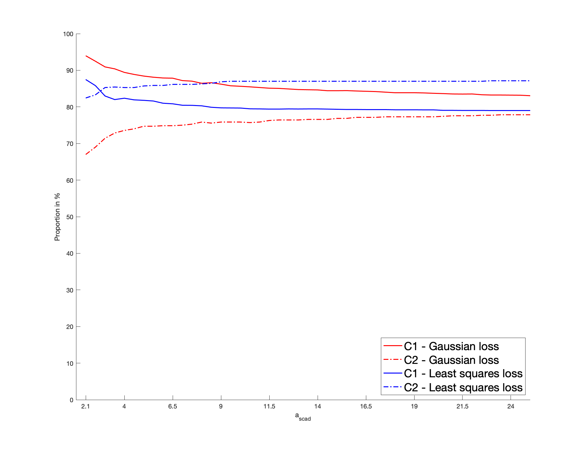
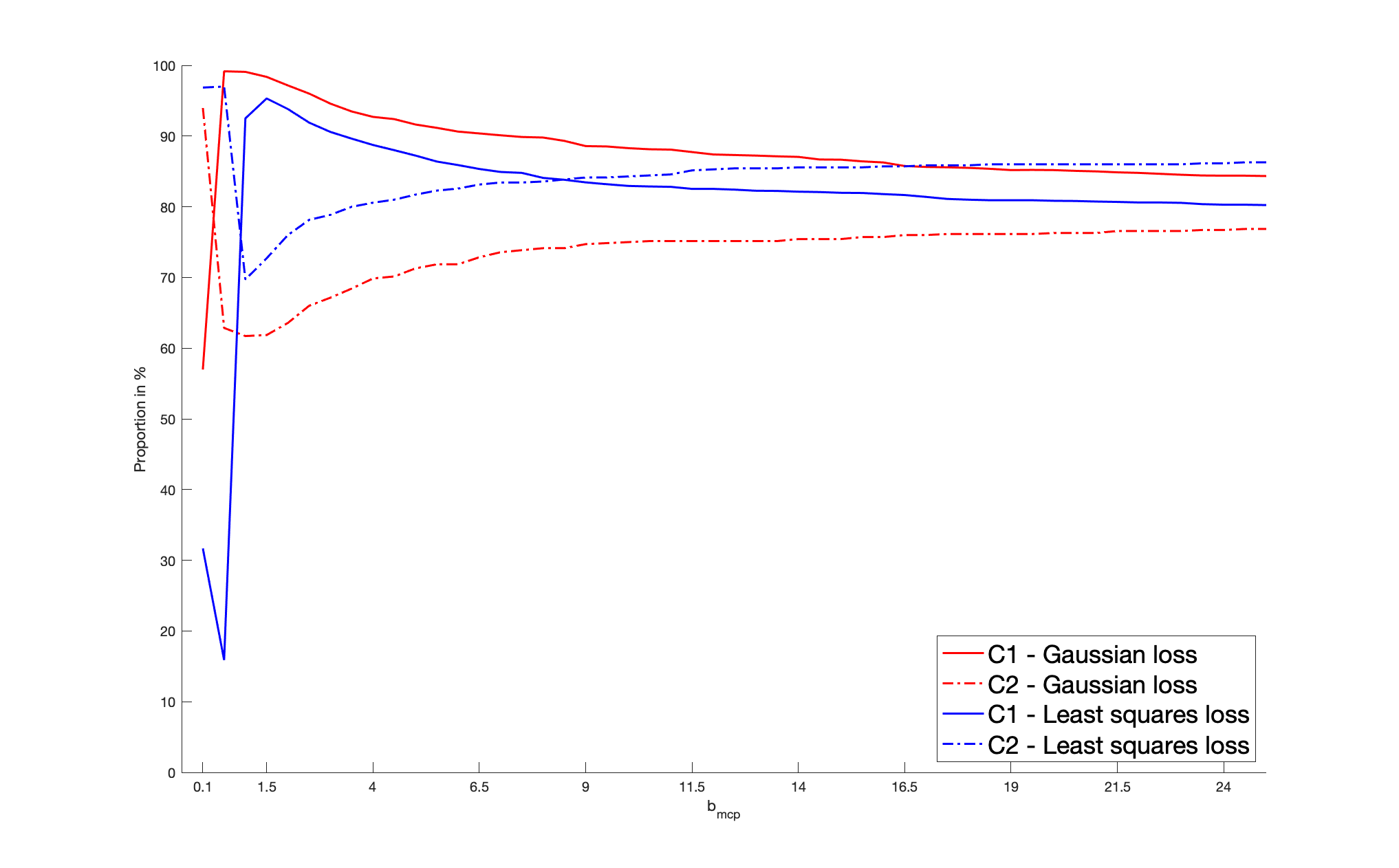
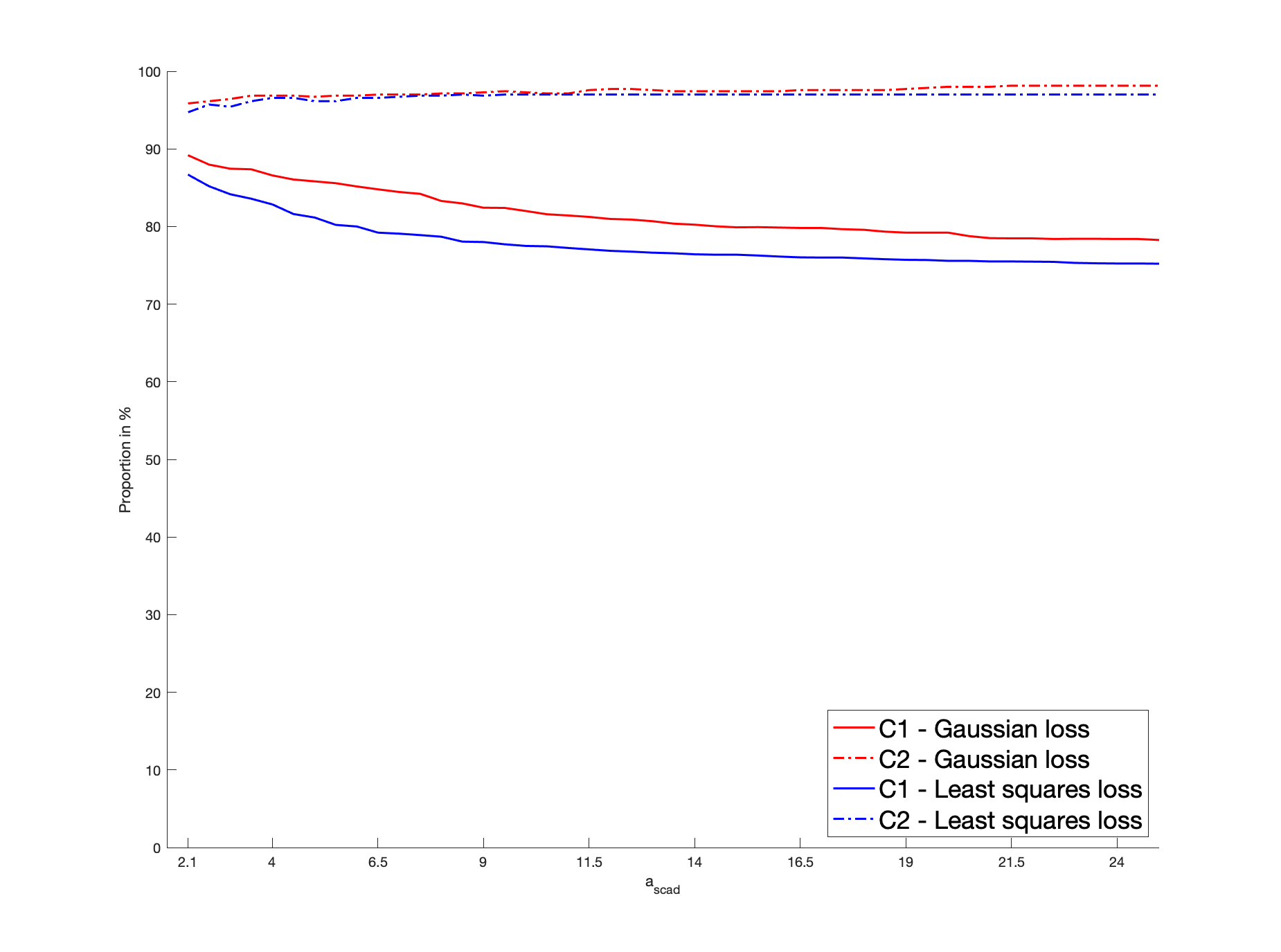
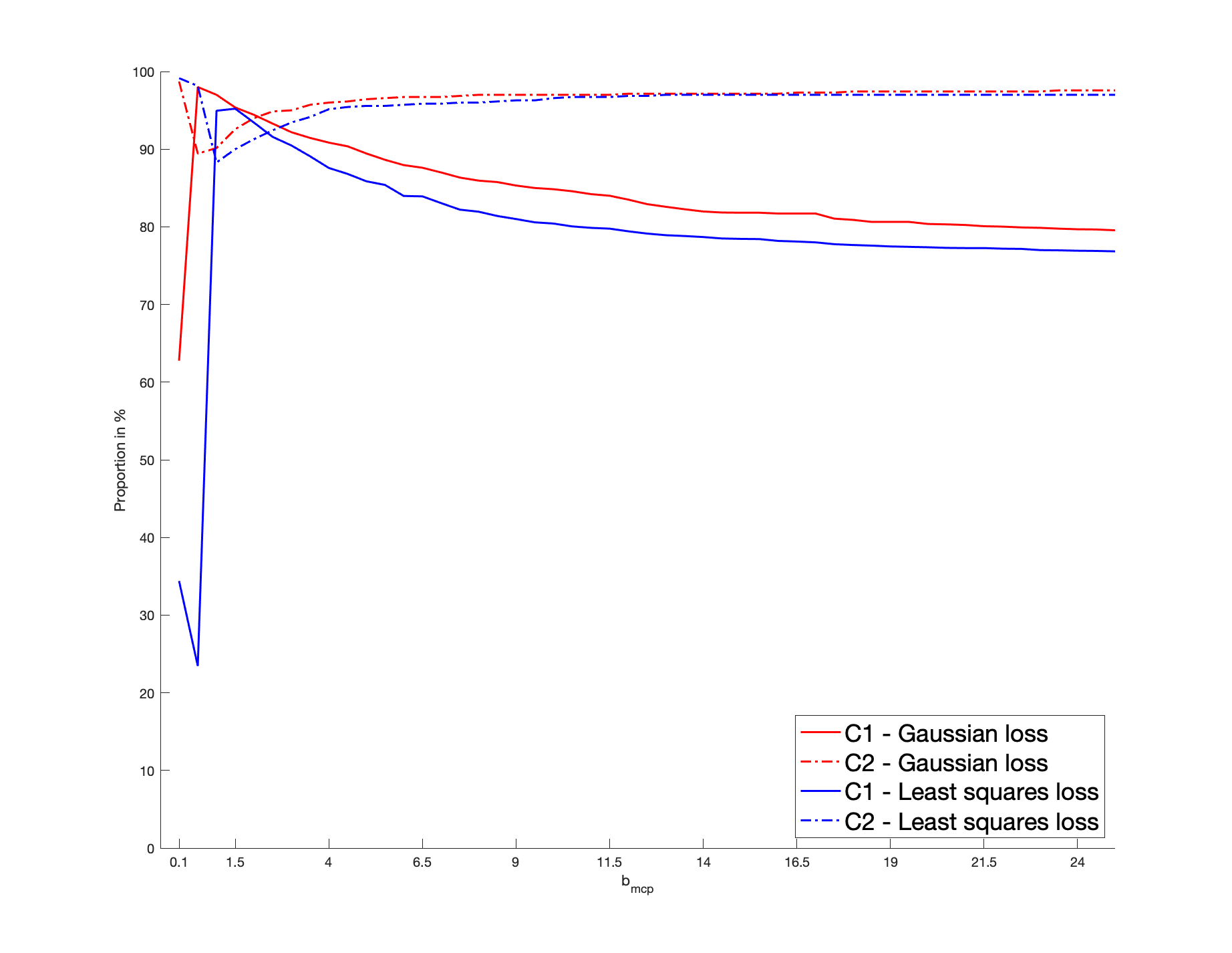
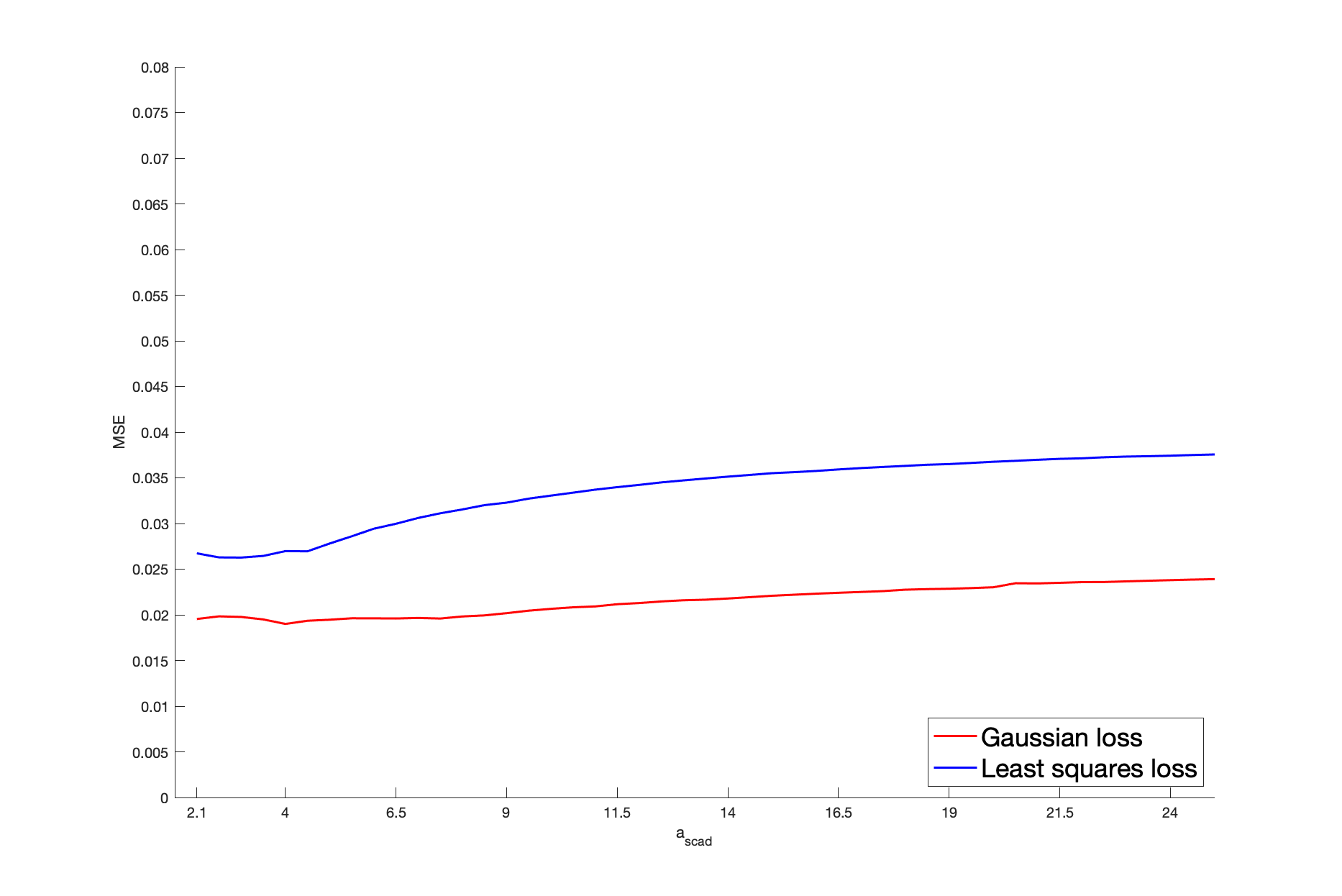
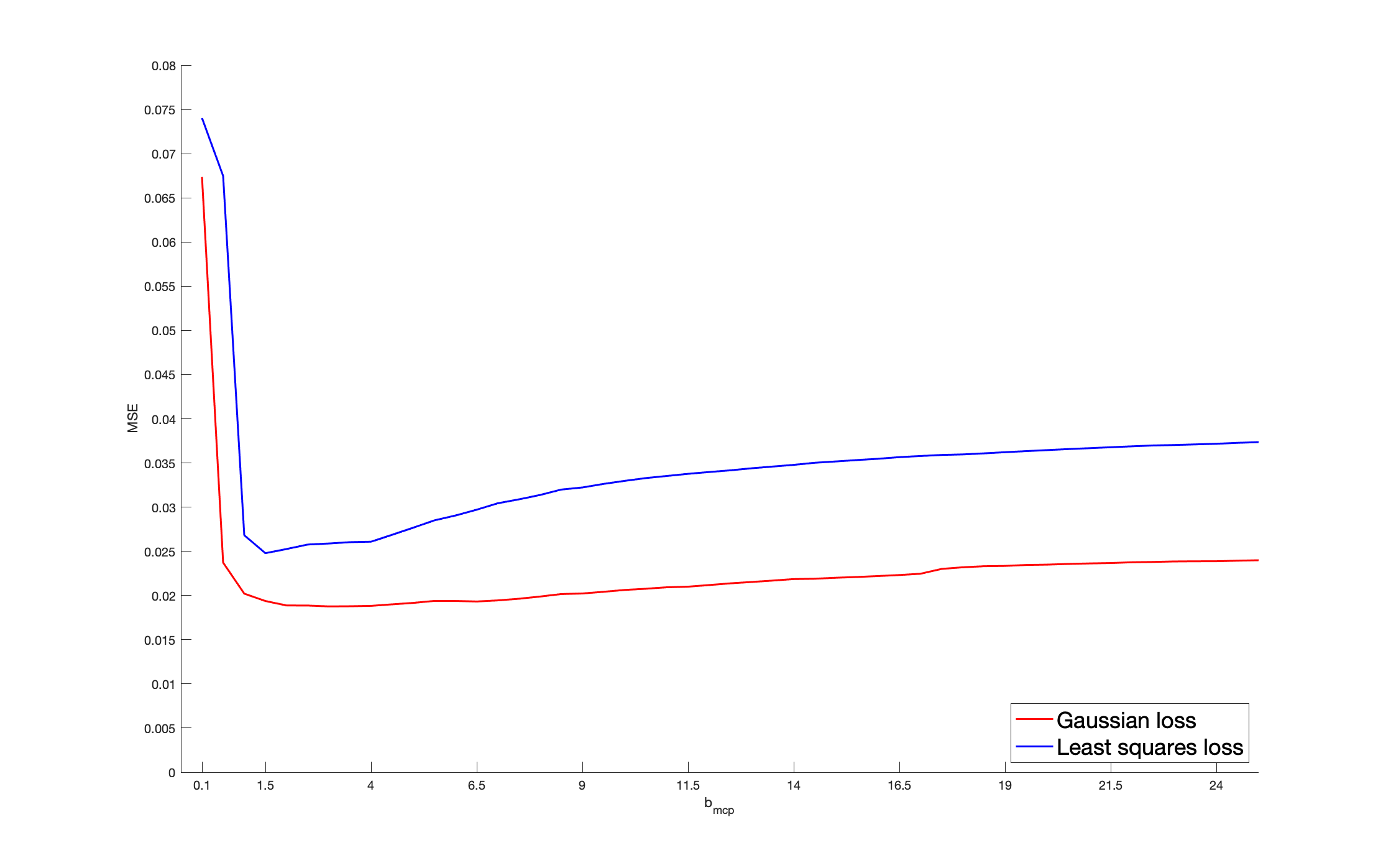
To be more specific, a sparse θ0\theta_{0} is randomly drawn for each batch as detailed below. Then, we generate a sample of nn vectors 𝑼i\mbox{\boldmath$U$}_{i} as follows: we draw 𝑼i=(Ui,1,,Ui,d)\mbox{\boldmath$U$}_{i}=(U_{i,1},\ldots,U_{i,d}), i{1,,n}i\in\{1,\ldots,n\}, from a Gaussian copula with parameter θ0\theta_{0}; then we consider their rank-based transformation to obtain a non-parametric estimator of their marginal distribution, providing the pseudo-observations 𝑼^i=(U^i,1,,U^i,d)\widehat{\mbox{\boldmath$U$}}_{i}=(\widehat{U}_{i,1},\ldots,\widehat{U}_{i,d}) that enter the loss function. Then, we solve (2.3). The non-penalized loss is the Gaussian log-likelihood, as defined in (5.1). Alternatively, in (2.3), we consider the least squares criterion for which (θ;U^i)=tr((𝒁ni𝒁niΣ)2)\ell(\theta;\widehat{U}_{i})=\text{tr}((\mbox{\boldmath$Z$}_{ni}\mbox{\boldmath$Z$}^{\top}_{ni}-\Sigma)^{2}), where 𝒁ni:=(Φ1(U^i,1),,Φ1(U^i,d))\mbox{\boldmath$Z$}_{ni}:=(\Phi^{-1}(\widehat{U}_{i,1}),\ldots,\Phi^{-1}(\widehat{U}_{i,d}))^{\top}. In both cases, the penalized problem is solved by a gradient descent algorithm based on the updating formulas of Section 4.2 in [24], where the initial value is set as S^:=n1i=1n𝐙ni𝐙ni\widehat{S}:=n^{-1}\sum^{n}_{i=1}\mathbf{Z}_{ni}\mathbf{Z}_{ni}^{\top}. The score for cross-validation purpose is defined in (5.2) with the Gaussian loss or the least squares loss. Concerning θ^\widehat{\theta}, we apply the SCAD, MCP and LASSO penalties. The non-convex SCAD and MCP ones require the calibration of ascada_{\text{scad}} and bmcpb_{\text{mcp}}, respectively. We select ascad=3.7a_{\text{scad}}=3.7, a “reference” value identified as optimal in [12] by cross-validated experiments. In the MCP case, the “reference” parameter is set as bmcp=3.5b_{\text{mcp}}=3.5, following [24]. We investigate the sensitivity of these non-convex procedures with respect to their parameters ascad,bmcpa_{\text{scad}},b_{\text{mcp}}. In particular, our results are also detailed with the values ascad=40a_{\text{scad}}=40 and bmcp=40b_{\text{mcp}}=40. This case corresponds to “large” ascada_{\text{scad}} and bmcpb_{\text{mcp}}, for which the corresponding penalty functions tend to the LASSO penalty.

We consider the dimensions d{10,20}d\in\{10,20\}, so that the dimension of θ0\theta_{0} is p=d(d1)/2=45p=d(d-1)/2=45 and 190190, respectively. The cardinality of the true support 𝒜{\mathcal{A}} is set arbitrarily as |𝒜|=7|{\mathcal{A}}|=7 (resp. |𝒜|=19|{\mathcal{A}}|=19) when d=10d=10 (resp. d=20d=20), so that the percentage of zero coefficients of θ0\theta_{0} is approximately 85%85\% (resp. 90%90\%). As for the non-zero coefficients of θ0\theta_{0}, for each batch, they are generated from the uniform distribution 𝒰([0.7,0.05][0.05,0.7]){\mathcal{U}}([-0.7,-0.05]\cup[0.05,0.7]), thus ensuring the minimum signal strength mink𝒜|θ0,k|0.05\min_{k\in{\mathcal{A}}}|\theta_{0,k}|\geq 0.05. As for the sample size, we consider n{500,1000}n\in\{500,1000\}. Note that, for each batch, the number of zero coefficients of θ0\theta_{0} remains unchanged but their locations may be different.

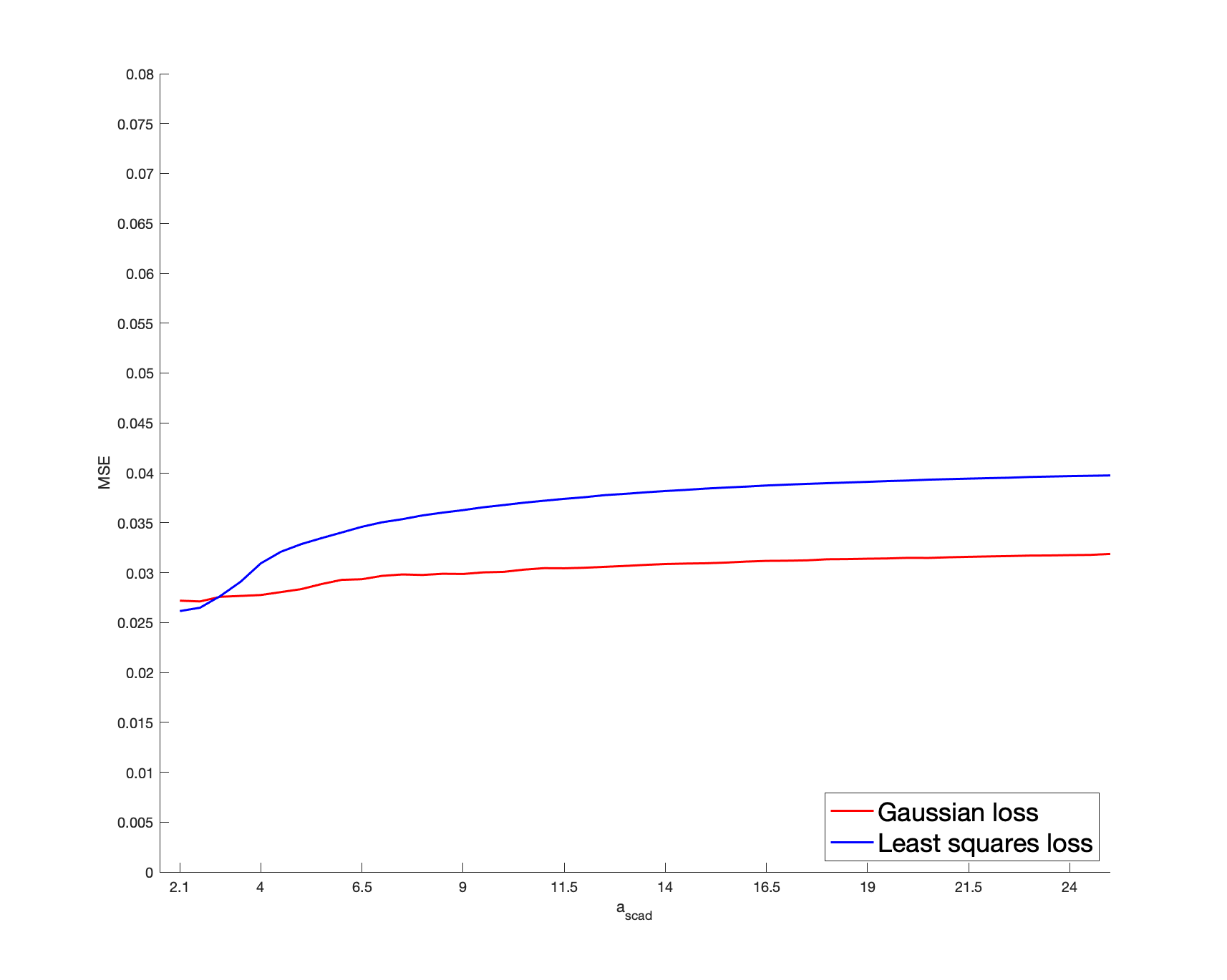
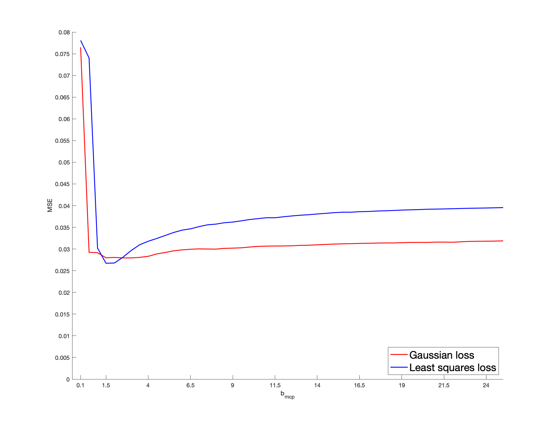
We report the variable selection performance through the percentage of zero coefficients in θ0\theta_{0} that are correctly estimated, denoted by C1, and the percentage of non-zero coefficients in θ0\theta_{0} correctly identified as such, denoted by C2. The mean squared error (MSE), defined as θ^θ022\|\widehat{\theta}-\theta_{0}\|^{2}_{2}, is reported as an estimation accuracy measure. These metrics are averaged over the two hundred batches and reported in Table 1. For clarifying the reading of the figures, the first entry 84.7084.70 in the column “Gaussian” represents the percentage of the true zero coefficients correctly identified by the estimator deduced from the Gaussian loss function, with SCAD penalization when ascad=3.7a_{\text{scad}}=3.7, for a sample size n=500n=500, a dimension d=10d=10, and averaged over two hundred batches; in the last MSE line, the value 0.06250.0625 in the column “Least Squares” represents the MSE of the estimator deduced from the least squares loss function with MCP penalization when bmcp=40b_{\text{mcp}}=40, for a sample size n=1000n=1000 and d=20d=20, and averaged over two hundred batches. Our results highlight that, for a given loss, the SCAD/MCP-based penalization procedures provide better results in terms of support recovery compared to the LASSO for our reference values of ascad,bmcpa_{\text{scad}},b_{\text{mcp}}. Furthermore, the SCAD and even more the MCP-based estimators with the Gaussian loss provide better recovery performances compared to the least squares loss. This is particularly true with the indicator C1, i.e., for the sake of identifying the zero coefficients. Interestingly, large ascad,bmcpa_{\text{scad}},b_{\text{mcp}} values worsen the recovery ability. Indeed, such large values result in a LASSO-type behavior, which is biased so that small λn\lambda_{n} will tend to be selected. Moreover, for any given penalty function, the Gaussian loss-based MSE’s are always lower than the least squares loss-based MSE’s, which suggest that the estimator deduced from the former loss is more efficient than the estimator obtained from the latter loss. Furthermore, larger ascad,bmcpa_{\text{scad}},b_{\text{mcp}} values worsen the MSE performances: when ascad=bmcp=40a_{\text{scad}}=b_{\text{mcp}}=40, for a given loss function, the MSE’s of SCAD/MCP are close to the LASSO. In Section I of the Appendix, we investigate further the sensitivity of the performances of the SCAD and MCP-based estimators with respect to ascada_{\text{scad}} and bmcpb_{\text{mcp}}.

Table 1: Model selection and accuracy, based on 200 replications. For each penalized loss, the results are reported according to the order SCAD, MCP and then LASSO. C1,C2\text{C1},\text{C2} are expressed in percentage, and larger numbers are better; for each MSE metric, smaller numbers are better.
(n,d,ascad,bmcp)(n,d,a_{\text{scad}},b_{\text{mcp}}) Truth Gaussian Least Squares
(500,10,3.7,3.5)(500,10,3.7,3.5) C1 100100 84.70 89.97 78.3684.70\,-\,89.97\,-\,78.36 80.22 86.26 73.7680.22\,-\,86.26\,-\,73.76
C2 100100 96.14 94.64 97.0796.14\,-\,94.64\,-\,97.07 95.57 94.43 96.0795.57\,-\,94.43\,-\,96.07
MSE 0.0190 0.0189 0.02380.0190\,-\,0.0189\,-\,0.0238 0.0293 0.0281 0.04210.0293\,-\,0.0281\,-\,0.0421
(1000,10,3.7,3.5)(1000,10,3.7,3.5) C1 100100 86.55 91.29 77.5386.55\,-\,91.29\,-\,77.53 80.37 86.90 69.1780.37\,-\,86.90\,-\,69.17
C2 100100 97.93 97.50 98.6497.93\,-\,97.50\,-\,98.64 98.14 97.64 98.7198.14\,-\,97.64\,-\,98.71
MSE 0.0081 0.0079 0.01170.0081\,-\,0.0079\,-\,0.0117 0.0131 0.0124 0.02130.0131\,-\,0.0124\,-\,0.0213
(500,10,40,40)(500,10,40,40) C1 100100 79.54 80.01 78.3679.54\,-\,80.01\,-\,78.36 74.30 75.34 73.7674.30\,-\,75.34\,-\,73.76
C2 100100 97.00 96.79 97.0797.00\,-\,96.79\,-\,97.07 96.00 95.93 96.0796.00\,-\,95.93\,-\,96.07
MSE 0.0228 0.0227 0.02380.0228\,-\,0.0227\,-\,0.0238 0.0405 0.0403 0.04210.0405\,-\,0.0403\,-\,0.0421
(1000,10,40,40)(1000,10,40,40) C1 100100 78.97 79.86 77.5378.97\,-\,79.86\,-\,77.53 70.49 71.54 69.1770.49\,-\,71.54\,-\,69.17
C2 100100 98.64 98.57 98.6498.64\,-\,98.57\,-\,98.64 98.64 98.57 98.7198.64\,-\,98.57\,-\,98.71
MSE 0.0110 0.0110 0.01170.0110\,-\,0.0110\,-\,0.0117 0.0199 0.0198 0.02130.0199\,-\,0.0198\,-\,0.0213
(500,20,3.7,3.5)(500,20,3.7,3.5) C1 100100 88.08 92.71 85.6388.08\,-\,92.71\,-\,85.63 84.13 89.91 81.1484.13\,-\,89.91\,-\,81.14
C2 100100 94.55 92.84 95.4094.55\,-\,92.84\,-\,95.40 94.05 92.55 94.8294.05\,-\,92.55\,-\,94.82
MSE 0.0602 0.0571 0.06900.0602\,-\,0.0571\,-\,0.0690 0.0937 0.0884 0.12720.0937\,-\,0.0884\,-\,0.1272
(1000,20,3.7,3.5)(1000,20,3.7,3.5) C1 100100 89.28 93.46 84.6589.28\,-\,93.46\,-\,84.65 86.16 91.77 80.3386.16\,-\,91.77\,-\,80.33
C2 100100 97.92 97.08 98.2197.92\,-\,97.08\,-\,98.21 97.11 96.13 97.7497.11\,-\,96.13\,-\,97.74
MSE 0.0252 0.0239 0.03370.0252\,-\,0.0239\,-\,0.0337 0.0433 0.0406 0.06640.0433\,-\,0.0406\,-\,0.0664
(500,20,40,40)(500,20,40,40) C1 100100 85.85 86.51 85.6385.85\,-\,86.51\,-\,85.63 81.29 82.14 81.1481.29\,-\,82.14\,-\,81.14
C2 100100 95.37 95.26 95.4095.37\,-\,95.26\,-\,95.40 94.79 94.58 94.8294.79\,-\,94.58\,-\,94.82
MSE 0.0673 0.0668 0.06900.0673\,-\,0.0668\,-\,0.0690 0.1234 0.1224 0.12720.1234\,-\,0.1224\,-\,0.1272
(1000,20,40,40)(1000,20,40,40) C1 100100 85.51 86.11 84.6585.51\,-\,86.11\,-\,84.65 80.73 81.74 80.3380.73\,-\,81.74\,-\,80.33
C2 100100 98.08 98.05 98.2198.08\,-\,98.05\,-\,98.21 97.74 97.55 97.7497.74\,-\,97.55\,-\,97.74
MSE 0.0322 0.0319 0.03370.0322\,-\,0.0319\,-\,0.0337 0.0631 0.0625 0.06640.0631\,-\,0.0625\,-\,0.0664

5.2.3 Conditional copulas

Our next application is dedicated to the sparse estimation of conditional copula models with known link functions and known marginal laws of the covariates: the experiment is an application of the penalized problem detailed in Subsection 4.1. We specify the law of 𝑿d\mbox{\boldmath$X$}\in{\mathbb{R}}^{d}, given some covariates 𝒁q\mbox{\boldmath$Z$}\in{\mathbb{R}}^{q}, as a parametric copula with parameter θ(𝒁β)\theta(\mbox{\boldmath$Z$}^{\top}\beta), where 𝒁q\mbox{\boldmath$Z$}\in{\mathbb{R}}^{q} and βq\beta\in{\mathbb{R}}^{q} (p=1p=1 and m=qm=q, with our notations of Section 4). We assume the marginal distribution of XkX_{k}, k{1,,d}k\in\{1,\ldots,d\}, is unknown and does not depend on 𝒁Z. We focus on the Clayton and Gumbel copulas, and restrict ourselves to d=2d=2.

In the same vein as in the previous application to sparse Gaussian copulas, for each sample size nn, we draw two hundred independent batches of nn vectors 𝑼i\mbox{\boldmath$U$}_{i} as follows: in each batch, we simulate a sparse true β0\beta_{0}; then for every i{1,,n}i\in\{1,\ldots,n\}, we draw the covariates Zi,kZ_{i,k}, k{1,,q}k\in\{1,\ldots,q\}, from a uniform distribution 𝒰([0,1]){\mathcal{U}}([0,1]), independently of each other; then, for a given 𝒁i=(Zi,1,,Zi,q)\mbox{\boldmath$Z$}_{i}=(Z_{i,1},\ldots,Z_{i,q})^{\top}, we sample 𝑼i=(Ui,1,Ui,2)\mbox{\boldmath$U$}_{i}=(U_{i,1},U_{i,2}) from the Clayton/Gumbel copula with parameter θi:=θ(𝒁iβ0)\theta_{i}:=\theta(\mbox{\boldmath$Z$}^{\top}_{i}\beta_{0}); we consider their rank-based transformation to obtain the pseudo-observations 𝑼^i=(U^i,1,U^i,2)\widehat{\mbox{\boldmath$U$}}_{i}=(\widehat{U}_{i,1},\widehat{U}_{i,2}), which are plugged in the penalized criterion. Here, the copula parameters θi\theta_{i} are specified in terms of Kendall’s tau: for each ii, define the Kendall’s tau τi:=2arctan(𝒁iβ0)/π\tau_{i}:=2\arctan(\mbox{\boldmath$Z$}^{\top}_{i}\beta_{0})/\pi. Using the mappings of, e.g., [26], set θi=2τi/(1τi)\theta_{i}=2\tau_{i}/(1-\tau_{i}) for the Clayton copula and θi=1/(1τi)\theta_{i}=1/(1-\tau_{i}) for the Gumbel copula. We consider the dimension q=30q=30, and set the cardinality of the true support 𝒜={k:β0,k0,k=1,,q}{\mathcal{A}}=\{k:\beta_{0,k}\neq 0,k=1,\cdots,q\} as |𝒜|=3|{\mathcal{A}}|=3, so that approximately 90%90\% of the entries of β0\beta_{0} are zero coefficients. For each batch, the non-zero entries are simulated from the uniform distribution 𝒰([0.05,1]){\mathcal{U}}([0.05,1]), which ensures that the following copula parameter constraints are satisfied: θi>0\theta_{i}>0 (resp. θi>1\theta_{i}>1) for the Clayton (resp. Gumbel) copula. For each batch, the locations of the zero/non-zero entries in β0\beta_{0} are arbitrary, but the size of 𝒜{\mathcal{A}} remains fixed. Finally, we consider the sample size n{500,1000}n\in\{500,1000\}. For a given batch, our criterion becomes:

β^argminβΘ{𝕃n(θ;𝒰^n,𝒵n)+nk=1𝑞𝒑(λn,|θk|)},with𝕃n(θ;𝒰^n,𝒵n)=i=1𝑛lncθ(𝒁iβ)(U^i,1,U^i,2),\widehat{\beta}\,{\color[rgb]{0,0,0}\in}\,\underset{\beta\in\Theta}{\arg\;\min}\;\Big{\{}{\mathbb{L}}_{n}(\theta;\widehat{{\mathcal{U}}}_{n},\mathcal{Z}_{n})+n\overset{q}{\underset{k=1}{\sum}}\mbox{\boldmath$p$}(\lambda_{n},|\theta_{k}|)\Big{\}},\;\text{with}\;{\mathbb{L}}_{n}(\theta;\widehat{{\mathcal{U}}}_{n},\mathcal{Z}_{n})=-\overset{n}{\underset{i=1}{\sum}}\ln c_{\theta(\mbox{\boldmath$Z$}^{\top}_{i}\beta)}\big{(}\widehat{U}_{i,1},\widehat{U}_{i,2}\big{)},

where lncθ(𝒁iβ)(.)\ln c_{\theta(\mbox{\boldmath$Z$}^{\top}_{i}\beta)}(.) is the log-density of the Clayton/Gumbel copula with parameter θ(𝒁iβ)\theta(\mbox{\boldmath$Z$}^{\top}_{i}\beta). As for the penalty function, we consider the SCAD, MCP and LASSO penalty functions to estimate 𝒜{\mathcal{A}} and β\beta. Moreover, we choose ascad{3.7,10,20,40,70}a_{\text{scad}}\in\{3.7,10,20,40,70\} and bmcp{3.5,10,20,40,70}b_{\text{mcp}}\in\{3.5,10,20,40,70\}. To assess the finite sample performance of the penalization methods and as in Section 5.2.2, we report in Table 2 the percentage of zero coefficients correctly estimated (C1), the percentage of non-zero coefficients correctly identified (C2) and the mean squared error (MSE), averaged over the two hundred batches. For both models and low/large sample sizes, our results emphasize the poor performances of the LASSO penalization in terms of support recovery (correct identification of the zero coefficients). As for non-convex penalization, the trade-off between C1 and C2 is more indicative than in the application to the Gaussian copula: small ascad,bmcpa_{\text{scad}},b_{\text{mcp}} provide better C1 to the detriment of C2, which results in larger MSE since C2 worsens in that case. The MSE results are significantly improved for nn large. Mid-range ascad,bmcpa_{\text{scad}},b_{\text{mcp}} values provide an optimal trade-off in terms of the combined C1, C2 and MSE metrics.

Table 2: Model selection and accuracy based on 200 replications. C1,C2\text{C1},\text{C2} are expressed in percentage, and larger numbers are better; for each MSE metric, smaller numbers are better.
  Gumbel n=500n=500 Gumbel n=1000n=1000   Clayton n=500n=500 Clayton n=1000n=1000
Penalty C1    C2    MSE C1    C2    MSE C1    C2    MSE C1    C2    MSE
SCAD, ascad=3.7a_{\text{scad}}=3.7 85.41 64.17 0.561285.41\;-\;64.17\;-\;0.5612 90.11 75.33 0.296490.11\;-\;75.33\;-\;0.2964 82.57 59.83 0.625582.57\;-\;59.83\;-\;0.6255 94.20 75.67 0.185694.20\;-\;75.67\;-\;0.1856
ascad=10a_{\text{scad}}=10 84.46 63.83 0.586084.46\;-\;63.83\;-\;0.5860 87.02 74.00 0.260787.02\;-\;74.00\;-\;0.2607 83.72 58.83 0.602183.72\;-\;58.83\;-\;0.6021 90.33 77.17 0.180090.33\;-\;77.17\;-\;0.1800
ascad=20a_{\text{scad}}=20 86.07 63.33 0.571186.07\;-\;63.33\;-\;0.5711 87.93 78.50 0.246487.93\;-\;78.50\;-\;0.2464 82.94 61.17 0.603782.94\;-\;61.17\;-\;0.6037 90.87 80.83 0.158490.87\;-\;80.83\;-\;0.1584
ascad=40a_{\text{scad}}=40 83.46 69.33 0.524683.46\;-\;69.33\;-\;0.5246 83.70 83.67 0.228083.70\;-\;83.67\;-\;0.2280 80.70 65.33 0.560280.70\;-\;65.33\;-\;0.5602 87.57 85.33 0.145687.57\;-\;85.33\;-\;0.1456
ascad=70a_{\text{scad}}=70 82.11 72.50 0.483482.11\;-\;72.50\;-\;0.4834 79.50 86.17 0.229779.50\;-\;86.17\;-\;0.2297 78.72 67.67 0.532278.72\;-\;67.67\;-\;0.5322 84.59 86.17 0.146284.59\;-\;86.17\;-\;0.1462
MCP, bmcp=3.5b_{\text{mcp}}=3.5 88.04 58.50 0.643088.04\;-\;58.50\;-\;0.6430 94.98 69.00 0.339694.98\;-\;69.00\;-\;0.3396 86.41 53.33 0.729586.41\;-\;53.33\;-\;0.7295 95.78 71.67 0.204495.78\;-\;71.67\;-\;0.2044
bmcp=10b_{\text{mcp}}=10 83.22 62.00 0.580983.22\;-\;62.00\;-\;0.5809 88.98 71.50 0.256388.98\;-\;71.50\;-\;0.2563 84.06 58.00 0.584684.06\;-\;58.00\;-\;0.5846 92.26 72.17 0.165392.26\;-\;72.17\;-\;0.1653
bmcp=20b_{\text{mcp}}=20 84.17 63.83 0.571184.17\;-\;63.83\;-\;0.5711 89.74 77.00 0.238689.74\;-\;77.00\;-\;0.2386 81.89 61.17 0.592781.89\;-\;61.17\;-\;0.5927 92.35 79.67 0.144292.35\;-\;79.67\;-\;0.1442
bmcp=40b_{\text{mcp}}=40 83.43 69.33 0.523483.43\;-\;69.33\;-\;0.5234 84.65 82.50 0.221184.65\;-\;82.50\;-\;0.2211 79.89 66.17 0.551379.89\;-\;66.17\;-\;0.5513 90.11 84.67 0.138590.11\;-\;84.67\;-\;0.1385
bmcp=70b_{\text{mcp}}=70 81.33 72.67 0.484481.33\;-\;72.67\;-\;0.4844 81.06 87.17 0.224981.06\;-\;87.17\;-\;0.2249 77.48 68.50 0.531277.48\;-\;68.50\;-\;0.5312 85.43 85.33 0.147685.43\;-\;85.33\;-\;0.1476
LASSO 76.87 79.00 0.409276.87\;-\;79.00\;-\;0.4092 72.52 88.33 0.224572.52\;-\;88.33\;-\;0.2245 76.00 74.33 0.438476.00\;-\;74.33\;-\;0.4384 77.65 89.00 0.139877.65\;-\;89.00\;-\;0.1398

6 Conclusion

We studied the asymptotic properties of sparse M-estimator based on pseudo-observations, where we treat the marginal distributions entering the loss function as unknown, which is a common situation in copula inference. Our framework includes, among others, semi-parametric copula models and the CML inference method. We assume sparsity among the coefficients of the true copula parameter and apply a penalty function to recover the sparse underlying support. Our method is based on penalized M-estimation and accommodates data-dependent penalties, such as the LASSO, SCAD and MCP. We establish the consistency of the sparse M-estimator together with the oracle property for the SCAD and MCP cases for both fixed and diverging dimensions of the vector of parameters. Because of the presence of non-parametric estimators of marginal cdfs’ and potentially unbounded loss functions, it is difficult to exhibit simple regularity conditions and to derive the oracle property. This would make the large sample analysis intricate when pp and dd simultaneously diverge. We shall leave it as a future research direction. Among potential applications of our methodology, the (brute force) estimation of vine models ([10]) under sparsity seems to be particularly relevant. Nonetheless, checking our regularity assumptions for such highly nonlinear models would surely be challenging. In addition, it would be interesting to prove similar theoretical results in the case of conditional copulas for which their conditional margins would depend on covariates.

Acknowledgements

J.D. Fermanian was supported by the labex Ecodec (reference project ANR-11-LABEX-0047) and B. Poignard by the Japanese Society for the Promotion of Science (Grant 22K13377).

References

  • [1] Abadir, K.M. and J.R. Magnus (2005). Matrix algebra. Cambridge University Press.
  • [2] Abegaz, F., Gijbels, I. and N. Veraverbeke (2012). Semiparametric estimation of conditional copulas. Journal of Multivariate Analysis, 110: 43–73.
  • [3] Abramowitz, Milton and I.A. Stegun (1972). Handbook of mathematical functions with formulas, graphs, and mathematical tables, Vol. 55, Reprint of the 1972 ed. A Wiley-Interscience Publication. Selected Government Publications, John Wiley & Sons, New York.
  • [4] Aistleitner, C. and J. Dick (2015). Functions of bounded variation, signed measures, and a general Koksma-Hlawka inequality. Acta Arithmetica, 167:143–171.
  • [5] Bühlmann, P. and S. van de Geer (2011). Statistics for high-dimensional data: Methods, theory and applications. 1st ed. Springer Series in Statistics. Springer, Berlin.
  • [6] Berghaus, B. and Bücher, A. and S. Volgushev (2017). Weak convergence of the empirical copula process with respect to weighted metrics. Bernoulli, 23(1):743–772.
  • [7] Cai, Z. and X. Wang (2014). Selection of mixed copula model via penalized likelihood. Journal of the American statistical Association, 109(506):788–801.
  • [8] Chen, X. and Y. Fan (2005). Pseudo-likelihood ratio tests for semiparametric multivariate copula model selection. Canadian Journal of Statistics, 33(3):389–414.
  • [9] Chen, X. and Y. Fan (2006). Estimation and model selection of semiparametric copula-based multivariate dynamic models under copula misspecification. Journal of econometrics, 135(1-2): 125–154.
  • [10] Czado, C (2019). Analyzing dependent data with vine copulas. 1st ed. Lecture Notes in Statistics. Springer, Cham.
  • [11] Dehling, H., Durieu, O. and M. Tusche (2014). Approximating class approach for empirical processes of dependent sequences indexed by functions. Bernoulli, 20(3):1372–1403.
  • [12] Fan, J. and R. Li (2001). Variable selection via nonconcave penalized likelihood and its oracle properties. Journal of the American statistical Association, 96(456):1348–1360.
  • [13] Fan, J. and H. Peng (2004). Nonconcave penalized likelihood with a diverging number of parameters. The Annals of Statistics, 32(3):928–961.
  • [14] Fermanian, J.-D. (1998). Contributions à l’analyse nonparamétrique des fonctions de hasard sur données multivariées et censurées. PhD thesis, Paris 6.
  • [15] Fermanian, J.-D., Radulović, D. and M. Wegkamp (2002). Weak convergence of empirical copula processes, Center for Research in Economics and Statistics, Working Paper, No. 2002-06.
  • [16] Fermanian, J.-D. and D. Radulović and M. Wegkamp (2004). Weak convergence of empirical copula processes. Bernoulli, 10(5):847–860.
  • [17] Fermanian, J.-D. and M. Wegkamp (2012). Time-dependent copulas. Journal of Multivariate Analysis, 110:19–29.
  • [18] Fermanian, J.D. and O. Lopez (2018). Single-index copulas. Journal of Multivariate Analysis, 165:27–55.
  • [19] Genest, C. and Ghoudi, K. and L.-P. Rivest (1995). A semi-parametric estimation procedure of dependence parameters in multivariate families of distributions. Biometrika, 82(3):543–552.
  • [20] Ghoudi, K. and B. Rémillard (2004). Empirical processes based on pseudo-observations II: the multivariate case. Fields Institute Communications, 44:381–406.
  • [21] Gijbels, I., Veraverbeke, N. and O. Marel (2011). Conditional copulas, association measures and their applications. Computational Statistics & Data Analysis, 55(5), 1919–1932.
  • [22] Hamori, S., Motegi, K. and Z. Zhang (2019). Calibration estimation of semiparametric copula models with data missing at random. Journal of Multivariate Analysis, 173:85–109.
  • [23] Hastie, T., Tibshirani, R. and J. Friedman (2009). The elements of statistical learning: Data mining, inference, and prediction. 2nd ed.Springer Series in Statistics. Springer, New York.
  • [24] Loh, P.L and M.J. Wainwright (2015). Regularized M-estimators with non-convexity: statistical and algorithmic theory for local optima. Journal of Machine Learning Research, 16:559-616.
  • [25] Loh, P.L and M.J. Wainwright (2017). Support recovery without incoherence: A case for nonconvex regularization. The Annals of Statistics, 45(6):2455–2482.
  • [26] Nelsen, R.B. (2006). An introduction to copulas. 2nd ed. Springer Series in Statistics. Springer, New York.
  • [27] Portnoy, S. (1985). Asymptotic behavior of M-estimators of pp regression parameters when p2/np^{2}/n is large; II. Normal approximation. The Annals of Statistics, 13(4):1403–1417.
  • [28] Radulović, D. and Wegkamp, M. and Y. Zhao (2017). Weak convergence of empirical copula processes indexed by functions. Bernoulli, 23(4B):3346–3384.
  • [29] Rémillard, B. and O. Scaillet (2009). Testing for equality between two copulas. Journal of Multivariate Analysis, 100(3):377–386.
  • [30] Ruymgaart, F.H. (1974). Asymptotic normality of nonparametric tests for independence. The Annals of Statistics, 2(5):892–910.
  • [31] Ruymgaart, F.H. and Shorack, G.R. and W.R. Van Zwet (1972). Asymptotic normality of nonparametric tests for independence. The Annals of Mathematical Statistics, 43(4):1122–1135.
  • [32] Segers, J. (2012). Asymptotics of empirical copula processes under non-restrictive smoothness assumptions. Bernoulli, 18(3):764–782.
  • [33] Shi, J. H. and T. Louis (1995). Inferences on the association parameter in copula models for bivariate survival data. Biometrics, 51(4):1384–1399.
  • [34] Tsukahara, H. (2005). Semi-parametric estimation in copula models. The Canadian Journal of Statistics, 33(3):357–375.
  • [35] van der Vaart, A.W. and J. Wellner (1996). Weak convergence and empirical processes: with applications to statistics. 1st ed. Springer Series in Statistics. Springer, New York.
  • [36] van der Vaart, A.W. and J.A. Wellner (2007). Empirical processes indexed by estimated functions. Asymptotics: Particles, Processes and Inverse Problems, 234–252, IMS Lecture Notes Monograph Series, 55.
  • [37] Yang, B. and Hafner, C.M. and Liu, G. and W. Long (2021). Semi-parametric estimation and variable selection for single-index copula models. Journal of Applied Econometrics, 36(7):962–988.
  • [38] Zhang, C.-H. (2010). Nearly unbiased variable selection under minimax concave penalty. The Annals of Statistics, 38(2):894-942.
  • [39] Zhang, S. and O. Okhrin and Q.M. Zhou and P.X.-K. Song (2016). Goodness-of-fit test for specification of semiparametric copula dependence models. Journal of Econometrics, 193(1):215–233.
  • [40] Zou, H. (2006). The adaptive lasso and its oracle properties. Journal of the American statistical association, 101(476):1418–1429.

Appendix A Multivariate rank statistics and empirical copula processes indexed by functions

In this section, we prove some theoretical results about the asymptotic behavior of multivariate rank statistics

f𝑑C^n=1ni=1nf(Fn,1(Xi,1),,Fn,d(Xi,d)),\int fd\widehat{C}_{n}=\frac{1}{n}\sum_{i=1}^{n}f\big{(}F_{n,1}(X_{i,1}),\ldots,F_{n,d}(X_{i,d})\big{)},

for a class of maps f:(0,1)df:(0,1)^{d}\rightarrow{\mathbb{R}} that will be of “locally” bounded variation and sufficiently regular. Such maps will be allowed to diverge when some of their arguments tend to zero or one, i.e. when their arguments are close to the boundaries of (0,1)d(0,1)^{d}. We will prove the asymptotic normality of f𝑑C^n\int fd\widehat{C}_{n}, extending Theorem 3.3 of [6] to any dimension d2d\geq 2. Moreover, we will state the weak convergence nfd(C^nC)\sqrt{n}\int fd(\widehat{C}_{n}-C) seen as an empirical process indexed by ff\in{\mathcal{F}}, for a convenient family of maps {\mathcal{F}}.

To be specific, consider a family of measurable maps ={f:(0,1)d}{\mathcal{F}}=\{f:(0,1)^{d}\rightarrow{\mathbb{R}}\}. As in [6] and for any ω0\omega\geq 0, define the weight function

gω,d(𝒖):=min{mink=1,,duk,1minj1uj,,1minjduj}ω,𝒖[0,1]d.g_{\omega,d}(\mbox{\boldmath$u$}):=\min\{\min_{k=1,\ldots,d}u_{k},1-\min_{j\neq 1}u_{j},\ldots,1-\min_{j\neq d}u_{j}\}^{\omega},\;\mbox{\boldmath$u$}\in[0,1]^{d}.

When u1u2udu_{1}\leq u_{2}\leq\cdots\leq u_{d}, check that gω,2(𝒖)=min(u1,1u2)g_{\omega,2}(\mbox{\boldmath$u$})=\min(u_{1},1-u_{2}). Moreover, if d=2d=2, then gω,2(u1,u2)=min(u1,u2,1u1,1u2)g_{\omega,2}(u_{1},u_{2})=\min(u_{1},u_{2},1-u_{1},1-u_{2}). To lighten notations and when there will be no ambiguity, the map gω,dg_{\omega,d} will simply denoted as gωg_{\omega} hereafter. For technical reasons, we will need the map g~ω(𝒖):=gω(𝒖)+𝟏(gω(𝒖)=0)\tilde{g}_{\omega}(\mbox{\boldmath$u$}):=g_{\omega}(\mbox{\boldmath$u$})+{\mathbf{1}}(g_{\omega}(\mbox{\boldmath$u$})=0) for every 𝒖[0,1]d\mbox{\boldmath$u$}\in[0,1]^{d}.

Recall the process ^n:=n(C^nC)\widehat{\mathbb{C}}_{n}:=\sqrt{n}(\widehat{C}_{n}-C) and ^n(f)=f𝑑^n\widehat{\mathbb{C}}_{n}(f)=\int f\,d\widehat{\mathbb{C}}_{n} for any ff\in{\mathcal{F}}. Therefore, ^n\widehat{\mathbb{C}}_{n} may be considered as a process defined on {\mathcal{F}}. The maps ff\in{\mathcal{F}} may potentially be unbounded, particularly when their arguments tend to the boundaries of the hypercube [0,1]d[0,1]^{d}. This is a common situation when ff is chosen as the log-density of many copula families. Moreover, we will need to apply an integration by parts trick that has proved its usefulness in several copula-related papers, particularly [28] and [6]. To this end, we introduce the following class of maps.

  • Definition.

    A map ff is of locally bounded Hardy Krause variation, a property denoted by fBHKVloc((0,1)d)f\in BHKV_{loc}\big{(}(0,1)^{d}\big{)}, if, for any sequence (an)(a_{n}) and (bn)(b_{n}), 0<an<bn<10<a_{n}<b_{n}<1, an0a_{n}\rightarrow 0, bn1b_{n}\rightarrow 1, the restriction of ff to [an,bn]d[a_{n},b_{n}]^{d} is of bounded Hardy-Krause variation.

The concept of Hardy-Krause variation has become a standard extension of the usual concept of bounded variation for multivariate maps: see the Supplementary Material in [6] or Section 2 and Appendix A in [28], and the references therein.

Denote the box 𝑩n,m:=(1/2n;11/2n]m\mbox{\boldmath$B$}_{n,m}:=(1/2n;1-1/2n]^{m} and 𝑩n,mc\mbox{\boldmath$B$}^{c}_{n,m} its complementary in [0,1]m[0,1]^{m}, 1<md1<m\leq d. Moreover, any sub-vector whose components are all equal to 1/2n1/2n (resp. 11/2n1-1/2n) will be denoted as 𝒄n\mbox{\boldmath$c$}_{n} (resp. 𝒅n\mbox{\boldmath$d$}_{n}). For any fBHKVloc((0,1)d)f\in BHKV_{loc}\big{(}(0,1)^{d}\big{)} and a measurable map g:(0,1)dg:(0,1)^{d}\rightarrow{\mathbb{R}}, the integral (0,1)dg𝑑f\int_{(0,1)^{d}}g\,df can be conveniently defined: see [6], Section 3.1 and its Supplementary Material.

In terms of notations, we use the same rules as [28], Section 1.1, to manage sub-vectors and the way of concatenating them. More precisely, for J{1,,d}J\subset\{1,\ldots,d\}, |J||J| denotes the cardinality of JJ, and the unary minus refers to the complement with respect to {1,,d}\{1,\ldots,d\} so that J={1,,d}J-J=\{1,\ldots,d\}\setminus J. For J{1,,d}J\subset\{1,\ldots,d\}, 𝒖J\mbox{\boldmath$u$}_{J} denotes a |J||J|-tuple of real numbers whose elements are uj,jJu_{j},j\in J; the vector 𝒖J\mbox{\boldmath$u$}_{J} typically belongs to [0,1]|J|[0,1]^{|J|}. Now let J1,J2{1,,d}J_{1},J_{2}\subset\{1,\ldots,d\}, J1J2=J_{1}\cap J_{2}=\emptyset and 𝒖,𝐯\mbox{\boldmath$u$},\mathbf{v} two vectors in [0,1]d[0,1]^{d}. The concatenation symbol “::” is defined as follows: the vector 𝒖J1:𝐯J2\mbox{\boldmath$u$}_{J_{1}}:\mathbf{v}_{J_{2}} denotes the point 𝒙[0,1]|J1J2|\mbox{\boldmath$x$}\in[0,1]^{|J_{1}\cup J_{2}|} such that xj=ujx_{j}=u_{j} for jJ1j\in J_{1} and xj=vjx_{j}=v_{j} for jJ2j\in J_{2}. The vector 𝒖J1:𝐯J2\mbox{\boldmath$u$}_{J_{1}}:\mathbf{v}_{J_{2}} is well defined for 𝒖J1[0,1]|J1|\mbox{\boldmath$u$}_{J_{1}}\in[0,1]^{|J_{1}|} and 𝐯J2[0,1]|J2|\mathbf{v}_{J_{2}}\in[0,1]^{|J_{2}|} when J1J2=J_{1}\cap J_{2}=\emptyset even if 𝒖J1\mbox{\boldmath$u$}_{-J_{1}} and 𝐯J2\mathbf{v}_{-J_{2}} remains unspecified. We use this concatenation symbol to glue together more than two sets of components: let 𝒖J1[0,1]|J1|,𝐯J2[0,1]|J2|,𝒘J3[0,1]|J3|\mbox{\boldmath$u$}_{J_{1}}\in[0,1]^{|J_{1}|},\mathbf{v}_{J_{2}}\in[0,1]^{|J_{2}|},\mbox{\boldmath$w$}_{J_{3}}\in[0,1]^{|J_{3}|} with J1,J2,J3J_{1},J_{2},J_{3} mutually disjoint sets such that J1J2J3={1,,d}J_{1}\cup J_{2}\cup J_{3}=\{1,\ldots,d\}. Then 𝒖J1:𝐯J2:𝒘J3\mbox{\boldmath$u$}_{J_{1}}:\mathbf{v}_{J_{2}}:\mbox{\boldmath$w$}_{J_{3}} is a well defined vector in [0,1]d[0,1]^{d}. Finally, for a function f:[0,1]df:[0,1]^{d}\rightarrow{\mathbb{R}} and a constant vector 𝐜J[0,1]|J|\mathbf{c}_{J}\in[0,1]^{|J|}, the function 𝒙f(𝒙J:𝐜J)\mbox{\boldmath$x$}_{\mapsto}f(\mbox{\boldmath$x$}_{J}:\mathbf{c}_{-J}) denotes a lower-dimensional projection of ff onto [0,1]|J|[0,1]^{|J|}. The integral of a function g:[0,1]|J|g:[0,1]^{|J|}\mapsto{\mathbb{R}} w.r.t. the measure induced by the latter map will be denoted as g(𝒙J)f(d𝒙J:𝐜J)\int g(\mbox{\boldmath$x$}_{J})\,f(d\mbox{\boldmath$x$}_{J}:\mathbf{c}_{-J}).

  • Definition.

    A family of maps {\mathcal{F}} is said to be regular with respect to the weight function gω,dg_{\omega,d} for some ω(0,1/2)\omega\in(0,1/2) (or gωg_{\omega}-regular, to be short) if

    • (i)

      every ff\in{\mathcal{F}} is BVHKloc((0,1)d)BVHK_{loc}\big{(}(0,1)^{d}\big{)} and right-continuous;

    • (ii)

      the map 𝒖supfminkmin(uk,1uk)ω|f(𝒖)|\mbox{\boldmath$u$}\mapsto\sup_{f\in{\mathcal{F}}}\min_{k}\min(u_{k},1-u_{k})^{\omega}|f(\mbox{\boldmath$u$})| is bounded on (0,1)d(0,1)^{d},

      supf(0,1)dgω,d(𝒖)|f(d𝒖)|<,\sup_{f\in{\mathcal{F}}}\int_{(0,1)^{d}}g_{\omega,d}(\mbox{\boldmath$u$})\,|f(d\mbox{\boldmath$u$})|<\infty, (A.1)

      and, for any partition (J1,J2,J3)(J_{1},J_{2},J_{3}) of the set of indices {1,,d}\{1,\ldots,d\} with J1J_{1}\neq\emptyset,

      supf𝑩n,|J1|gω,d(𝒖J1:𝒄n,J2:𝒅n,J3)|f(d𝒖J1:𝒄n,J2:𝒅n,J3)|=O(1).\sup_{f\in{\mathcal{F}}}\int_{\mbox{\boldmath$B$}_{n,|J_{1}|}}g_{\omega,d}(\mbox{\boldmath$u$}_{J_{1}}:\mbox{\boldmath$c$}_{n,J_{2}}:\mbox{\boldmath$d$}_{n,J_{3}}\big{)}\big{|}f\big{(}d\mbox{\boldmath$u$}_{J_{1}}:\mbox{\boldmath$c$}_{n,J_{2}}:\mbox{\boldmath$d$}_{n,J_{3}}\big{)}\big{|}=O(1). (A.2)

      Moreover, the latter sequence tends to zero when J2J_{2}\neq\emptyset.

When ={f0}{\mathcal{F}}=\{f_{0}\} is a singleton, one simply says that the map f0f_{0} is gωg_{\omega}-regular. Note that, if 𝒖J1𝑩n,|J1|\mbox{\boldmath$u$}_{J_{1}}\in\mbox{\boldmath$B$}_{n,|J_{1}|}, then gω,d(𝒖J1:𝒄n,J2:𝒅n,J3)=(2n)ωg_{\omega,d}(\mbox{\boldmath$u$}_{J_{1}}:\mbox{\boldmath$c$}_{n,J_{2}}:\mbox{\boldmath$d$}_{n,J_{3}}\big{)}=(2n)^{-\omega} except when J2=J_{2}=\emptyset and |J1|2|J_{1}|\geq 2 simultaneously. In the latter case, gω,d(𝒖J1:𝒅n,J1)=gω,|J1|(𝒖J1)g_{\omega,d}(\mbox{\boldmath$u$}_{J_{1}}:\mbox{\boldmath$d$}_{n,-J_{1}}\big{)}=g_{\omega,|J_{1}|}(\mbox{\boldmath$u$}_{J_{1}}).

Remark 2.

Consider a family {\mathcal{F}} of maps from (0,1)d(0,1)^{d} to {\mathbb{R}}. Assume there exist mm subsets Ik{1,,d}I_{k}\subset\{1,\ldots,d\}, k{1,,m}k\in\{1,\ldots,m\} s.t. every member ff\in{\mathcal{F}} can be written

f(𝒖)=f1,I1(𝒖I1)++fm,Im(𝒖Im),𝒖(0,1)d,f(\mbox{\boldmath$u$})=f_{1,I_{1}}(\mbox{\boldmath$u$}_{I_{1}})+\ldots+f_{m,I_{m}}(\mbox{\boldmath$u$}_{I_{m}}),\;\;\mbox{\boldmath$u$}\in(0,1)^{d},

for some maps fk,Ik:(0,1)|Ik|f_{k,I_{k}}:(0,1)^{|I_{k}|}\rightarrow{\mathbb{R}}, k{1,,m}k\in\{1,\ldots,m\}. Define k={fk,Ik;f}{\mathcal{F}}_{k}=\{f_{k,I_{k}};f\in{\mathcal{F}}\} for every kk. If every k{\mathcal{F}}_{k}, k{1,,m},k\in\{1,\ldots,m\}, is regular w.r.t. the weight function gω,|Ik|g_{\omega,|I_{k}|}, then it is easy to see that {\mathcal{F}} is regular w.r.t. the weight function gω,dg_{\omega,d}. This property may be invoked to prove the gωg_{\omega} regularity of the Gaussian copula family, for instance (see Section E in the Appendix).

Remark 3.

Any family {\mathcal{F}} of maps defined on (0,1)d(0,1)^{d} may formally be seen as a family ~\tilde{\mathcal{F}} of maps defined on a larger dimension, say (0,1)d+p(0,1)^{d+p}, p>0p>0: every ff\in{\mathcal{F}} defines a map f~\tilde{f} on (0,1)d+p(0,1)^{d+p} by setting f~(𝐮,𝐯)=f(𝐮)\tilde{f}(\mbox{\boldmath$u$},\mathbf{v})=f(\mbox{\boldmath$u$}), 𝐮(0,1)d\mbox{\boldmath$u$}\in(0,1)^{d}, 𝐯(0,1)p\mathbf{v}\in(0,1)^{p}. It can be easily checked that, if {\mathcal{F}} is gωg_{\omega} regular then this is still the case for ~\tilde{\mathcal{F}}.

Beside the regularity conditions on the family of maps {\mathcal{F}}, we will need that the (standard) empirical process αn\alpha_{n} is well-behaved. To this aim, we recall the so-called conditions 4.1, 4.2 and 4.3 in [6].

Assumption 10.

There exists κ1(0,1/2]{\color[rgb]{0,0,0}\kappa}_{1}\in(0,1/2] such that, for all μ(0,κ1)\mu\in(0,{\color[rgb]{0,0,0}\kappa}_{1}) and all sequences δn0\delta_{n}\rightarrow 0, we have

sup|𝒖𝐯|<δn|αn(𝒖)αn(𝐯)||𝒖𝐯|μnμ=oP(1).\sup_{|\mbox{\boldmath$u$}-\mathbf{v}|<\delta_{n}}\frac{|\alpha_{n}(\mbox{\boldmath$u$})-\alpha_{n}(\mathbf{v})|}{|\mbox{\boldmath$u$}-\mathbf{v}|^{\mu}\vee n^{-\mu}}=o_{P}(1).
Assumption 11.

There exists κ2(0,1/2]{\color[rgb]{0,0,0}\kappa}_{2}\in(0,1/2] and κ3(1/2,1]{\color[rgb]{0,0,0}\kappa}_{3}\in(1/2,1] such that, for any ν(0,κ2){\color[rgb]{0,0,0}\nu}\in(0,{\color[rgb]{0,0,0}\kappa}_{2}), any λ(0,κ3)\lambda\in(0,{\color[rgb]{0,0,0}\kappa}_{3}) and any j{1,,d}j\in\{1,\ldots,d\}, we have

supu(0,1)|n{Gnj(u)u}uν(1u)ν|+supu(1/nλ,11/nλ)|n{Gnj(u)u}uν(1u)ν|=OP(1).\sup_{u\in(0,1)}\Big{|}\frac{\sqrt{n}\big{\{}G_{nj}(u)-u\big{\}}}{u^{{\color[rgb]{0,0,0}\nu}}(1-u)^{{\color[rgb]{0,0,0}\nu}}}\Big{|}+\sup_{u\in(1/n^{\lambda},1-1/n^{\lambda})}\Big{|}\frac{\sqrt{n}\big{\{}G^{-}_{nj}(u)-u\big{\}}}{u^{{\color[rgb]{0,0,0}\nu}}(1-u)^{{\color[rgb]{0,0,0}\nu}}}\Big{|}=O_{P}(1).
Assumption 12.

The empirical process (αn)(\alpha_{n}) converges weakly in ([0,1]d)\ell^{\infty}([0,1]^{d}) to some limit process αC\alpha_{C} which has continuous sample paths, almost surely.

As pointed out in [6], such conditions 10-12 are satisfied for i.i.d. data with κ1=1/2{\color[rgb]{0,0,0}\kappa}_{1}=1/2, κ2=1/2{\color[rgb]{0,0,0}\kappa}_{2}=1/2 and κ3=1{\color[rgb]{0,0,0}\kappa}_{3}=1. In the latter case, the limiting process αC\alpha_{C} is a CC-Brownian bridge, such that cov{αC(𝒖),αC(𝐯)}=C(𝒖𝐯)C(𝒖)C(𝐯)\text{cov}\big{\{}\alpha_{C}(\mbox{\boldmath$u$}),\alpha_{C}(\mathbf{v})\big{\}}=C(\mbox{\boldmath$u$}\wedge\mathbf{v})-C(\mbox{\boldmath$u$})C(\mathbf{v}) for any 𝒖u and 𝐯\mathbf{v} in [0,1]d[0,1]^{d}, with the usual notation 𝒖𝐯=(min(u1,v1),,min(ud,vd))\mbox{\boldmath$u$}\wedge\mathbf{v}=\big{(}\min(u_{1},v_{1}),\ldots,\min(u_{d},v_{d})\big{)}. More generally, if the process (𝑿i)i(\mbox{\boldmath$X$}_{i})_{i\in{\mathbb{N}}} is strongly stationary and geometrically α\alpha-mixing, then the assumptions 10-12 are still satisfied, with the same choice κ1=1/2{\color[rgb]{0,0,0}\kappa}_{1}=1/2, κ2=1/2{\color[rgb]{0,0,0}\kappa}_{2}=1/2 and κ3=1{\color[rgb]{0,0,0}\kappa}_{3}=1 (Proposition 4.4 in [6]). In the latter case, the covariance of the limiting process is more complex: cov{αC(𝒖),αC(𝐯)}=jcov{𝟏(𝑼0𝒖),𝟏(𝑼j𝒖)}\text{cov}\big{\{}\alpha_{C}(\mbox{\boldmath$u$}),\alpha_{C}(\mathbf{v})\big{\}}=\sum_{j\in{\mathbb{Z}}}\text{cov}\big{\{}{\mathbf{1}}(\mbox{\boldmath$U$}_{0}\leq\mbox{\boldmath$u$}),{\mathbf{1}}(\mbox{\boldmath$U$}_{j}\leq\mbox{\boldmath$u$})\big{\}}.

Assumption 13.

For any I{1,,d}I\subset\{1,\ldots,d\}, II\neq\emptyset, any ff that belongs to a regular family {\mathcal{F}} and for any continuous map h:[0,1]|I|h:[0,1]^{|I|}\rightarrow{\mathbb{R}}, the sequence 𝐁n,|I|h(𝐮I)gω(𝐮I:𝐝n,I)f(d𝐮I:𝐝n,I)\int_{\mbox{\boldmath$B$}_{n,|I|}}h(\mbox{\boldmath$u$}_{I})g_{\omega}\big{(}\mbox{\boldmath$u$}_{I}:\mbox{\boldmath$d$}_{n,-I}\big{)}\,f\big{(}d\mbox{\boldmath$u$}_{I}:\mbox{\boldmath$d$}_{n,-I}\big{)} is convergent when nn\rightarrow\infty. Its limit is denoted as (0,1)|I|h(𝐮I)gω(𝐮I:𝟏I)f(d𝐮I:𝟏I)\int_{(0,1)^{|I|}}h(\mbox{\boldmath$u$}_{I})g_{\omega}\big{(}\mbox{\boldmath$u$}_{I}:{\mathbf{1}}_{-I}\big{)}\,f\big{(}d\mbox{\boldmath$u$}_{I}:{\mathbf{1}}_{-I}\big{)}, i.e. it is given by an integral w.r.t. a borelian measure on (0,1)|I|(0,1)^{|I|} denoted as f(:𝟏I)f\big{(}\cdot:{\mathbf{1}}_{-I}\big{)}.

The latter regularity condition is required to get the weak convergence of our main statistic in Theorem A.1. Note that the map f(𝒖)f(\mbox{\boldmath$u$}) is not defined when one component of 𝒖u is one. Therefore, the way we write the limits in Assumption 13 is a slight abuse of notation. Typically, f(𝒖I:𝟏I)f(\mbox{\boldmath$u$}_{I}:{\mathbf{1}}_{-I}) will be defined as the limit f(𝒖I:𝐯I)f(\mbox{\boldmath$u$}_{I}:\mathbf{v}_{-I}) when 𝐯I\mathbf{v}_{-I} tends to 𝟏I{\mathbf{1}}_{-I} when such a limit exists. In other standard situations, there exists a measurable map hfh_{f} such that f(d𝒖I:𝒖I)=hf(𝒖)d𝒖If\big{(}d\mbox{\boldmath$u$}_{I}:\mbox{\boldmath$u$}_{-I}\big{)}=h_{f}(\mbox{\boldmath$u$})\,d\mbox{\boldmath$u$}_{I}. If it is possible to extend by continuity the map 𝒖gω(𝒖)hf(𝒖)\mbox{\boldmath$u$}\mapsto g_{\omega}(\mbox{\boldmath$u$})h_{f}(\mbox{\boldmath$u$}) when 𝒖I\mbox{\boldmath$u$}_{-I} tends to 𝟏I{\mathbf{1}}_{-I}, simply set gω(𝒖I:𝟏I)f(d𝒖I:𝟏I)=gω(𝒖I:𝟏I)hf(𝒖I:𝟏I)d𝒖Ig_{\omega}\big{(}\mbox{\boldmath$u$}_{I}:{\mathbf{1}}_{-I}\big{)}f\big{(}d\mbox{\boldmath$u$}_{I}:{\mathbf{1}}_{-I}\big{)}=g_{\omega}\big{(}\mbox{\boldmath$u$}_{I}:{\mathbf{1}}_{-I}\big{)}h_{f}(\mbox{\boldmath$u$}_{I}:{\mathbf{1}}_{-I})\,d\mbox{\boldmath$u$}_{I}. But other more complex situations.

To get the weak convergence of the process ^n\widehat{\mathbb{C}}_{n} indexed by the maps in {\mathcal{F}}, we will need to strengthen the latter assumption 13, so that it becomes true uniformly over {\mathcal{F}}.

Assumption 14.

For any I{1,,d}I\subset\{1,\ldots,d\} and any continuous map h:[0,1]|I|h:[0,1]^{|I|}\rightarrow{\mathbb{R}},

supf|𝑩n,|I|h(𝒖I)gω(𝒖I:𝒅n,I)f(d𝒖I:𝒅n,I)(0,1)|I|h(𝒖I)gω(𝒖I:𝟏I)f(d𝒖I:𝟏I)|0,\sup_{f\in{\mathcal{F}}}\big{|}\int_{\mbox{\boldmath$B$}_{n,|I|}}h(\mbox{\boldmath$u$}_{I})g_{\omega}\big{(}\mbox{\boldmath$u$}_{I}:\mbox{\boldmath$d$}_{n,-I}\big{)}\,f\big{(}d\mbox{\boldmath$u$}_{I}:\mbox{\boldmath$d$}_{n,-I}\big{)}-\int_{(0,1)^{|I|}}h(\mbox{\boldmath$u$}_{I})g_{\omega}\big{(}\mbox{\boldmath$u$}_{I}:{\mathbf{1}}_{-I}\big{)}\,f\big{(}d\mbox{\boldmath$u$}_{I}:{\mathbf{1}}_{-I}\big{)}\big{|}\longrightarrow 0,

when nn\rightarrow\infty.

Theorem A.1.

(i) Assume the assumptions 2,10 and 11 are satisfied and consider a family {\mathcal{F}} of maps that is gωg_{\omega}-regular, for some ω(0,min(κ12(1κ1),κ22(1κ2),κ31/2))\omega\in\big{(}0,\min(\frac{{\color[rgb]{0,0,0}\kappa}_{1}}{2(1-{\color[rgb]{0,0,0}\kappa}_{1})},\frac{{\color[rgb]{0,0,0}\kappa}_{2}}{2(1-{\color[rgb]{0,0,0}\kappa}_{2})},{\color[rgb]{0,0,0}\kappa}_{3}-1/2)\big{)}. Then, for any ff\in{\mathcal{F}}, we have

f𝑑^n=(1)d𝑩n,d¯n(𝒖)f(d𝒖)\displaystyle\int f\,d\widehat{\mathbb{C}}_{n}=(-1)^{d}\int_{\mbox{\boldmath$B$}_{n,d}}\bar{\mathbb{C}}_{n}(\mbox{\boldmath$u$})\,f\big{(}d\mbox{\boldmath$u$}\big{)} (A.3)
+\displaystyle+ I{1,,d}I,I{1,,d}(1)|I|𝑩n,|I|¯n(𝒖I:𝟏I)g~ω(𝒖I:𝟏I)gω(𝒖I:𝒅n,I)f(d𝒖I:𝒅n,I)+rn(f),\displaystyle\sum_{\begin{subarray}{c}I\subset\{1,\ldots,d\}\\ I\neq\emptyset,I\neq\{1,\ldots,d\}\end{subarray}}(-1)^{|I|}\int_{\mbox{\boldmath$B$}_{n,|I|}}\frac{\bar{\mathbb{C}}_{n}(\mbox{\boldmath$u$}_{I}:{\mathbf{1}}_{-I})}{\tilde{g}_{\omega}(\mbox{\boldmath$u$}_{I}:{\mathbf{1}}_{-I})}g_{\omega}\big{(}\mbox{\boldmath$u$}_{I}:\mbox{\boldmath$d$}_{n,-I}\big{)}\,f\big{(}d\mbox{\boldmath$u$}_{I}:\mbox{\boldmath$d$}_{n,-I}\big{)}+r_{n}(f),

where ¯n(𝐮):=αn(𝐮)k=1dC˙k(𝐮)αn(𝟏k:uk)\bar{\mathbb{C}}_{n}(\mbox{\boldmath$u$}):=\alpha_{n}(\mbox{\boldmath$u$})-\sum_{k=1}^{d}\dot{C}_{k}(\mbox{\boldmath$u$})\alpha_{n}({\mathbf{1}}_{-k}:u_{k}), 𝐮[0,1]d\mbox{\boldmath$u$}\in[0,1]^{d} and supf|rn(f)|=oP(1)\sup_{f\in{\mathcal{F}}}|r_{n}(f)|=o_{P}(1).

(ii) In addition, assume the conditions 12 and 13 apply. Then, for any function ff\in{\mathcal{F}}, the sequence of random variables nfd(C^nC)\sqrt{n}\int f\,d(\widehat{C}_{n}-C) tends in law to the centered Gaussian r.v.

(1)d(0,1)d(𝒖)f(d𝒖)+I{1,,d}I,I{1,,d}(1)|I|(0,1)|I|(𝒖I:𝟏I)f(d𝒖I:𝟏I),(-1)^{d}\int_{(0,1)^{d}}{\mathbb{C}}(\mbox{\boldmath$u$})\,f(d\mbox{\boldmath$u$})+\sum_{\begin{subarray}{c}I\subset\{1,\ldots,d\}\\ I\neq\emptyset,I\neq\{1,\ldots,d\}\end{subarray}}(-1)^{|I|}\int_{(0,1)^{|I|}}{\mathbb{C}}(\mbox{\boldmath$u$}_{I}:{\mathbf{1}}_{-I})\,f\big{(}d\mbox{\boldmath$u$}_{I}:{\mathbf{1}}_{-I}\big{)}, (A.4)

where (𝐮):=αC(𝐮)k=1dC˙k(𝐮)αC(𝟏k:uk){\mathbb{C}}(\mbox{\boldmath$u$}):=\alpha_{C}(\mbox{\boldmath$u$})-\sum_{k=1}^{d}\dot{C}_{k}(\mbox{\boldmath$u$})\alpha_{C}({\mathbf{1}}_{-k}:u_{k}) for any 𝐮[0,1]d\mbox{\boldmath$u$}\in[0,1]^{d}.

(iii) Under the latter assumptions of (i) and (ii), in addition to Assumption 14, ^n\widehat{\mathbb{C}}_{n} weakly tends in ()\ell^{\infty}({\mathcal{F}}) to a Gaussian process.

Points (i) and (ii) of the latter theorem yield a generalization of Theorem 3.3 in [6] for any arbitrarily chosen dimension d2d\geq 2, and uniformly over a class of functions. Note that it is always possible to set ={f0}{\mathcal{F}}=\{f_{0}\} and we have proved the weak convergence of a single multivariate rank statistic. The proof is based on the integration by part formula in [28]. Note that, in dimension d=2d=2, (u1,1)=(1,u2)=0{\mathbb{C}}(u_{1},1)={\mathbb{C}}(1,u_{2})=0 for any u1,u2(0,1)u_{1},u_{2}\in(0,1). Thus, in the bivariate case, the limiting law of nfd(C^nC)\sqrt{n}\int f\,d(\widehat{C}_{n}-C) is simply the law of (0,1)2𝑑f\int_{(0,1)^{2}}{\mathbb{C}}\,df, as stated in Theorem 3.3 in [6]. Nonetheless, this is no longer true in dimension d>2d>2, explaining the more complex limiting laws in our Theorem A.1. Finally, the sum in (A.4) can be restricted to the subsets II such that |I|2|I|\geq 2. Indeed, when II is a singleton, then (𝒖I:𝟏I){\mathbb{C}}(\mbox{\boldmath$u$}_{I}:{\mathbf{1}}_{-I}) is zero a.s.

The point (iii) of Theorem A.1 extends Theorem 5 in [28]. The latter one was restricted to right-continuous maps ff of bounded Hardy-Krause variation and defined on the whole hypercube [0,1]d[0,1]^{d}. For any of these maps ff, there exists a finite signed Borel measure bounded νf\nu_{f} on [0,1]d[0,1]^{d} such that f(𝒖)=νf([𝟎,𝒖])f(\mbox{\boldmath$u$})=\nu_{f}\big{(}[{\mathbf{0}},\mbox{\boldmath$u$}]\big{)} for every 𝒖[0,1]d\mbox{\boldmath$u$}\in[0,1]^{d} (Theorem 3 in [4]). In particular, they are bounded on [0,1]d[0,1]^{d}, an excessively demanding assumption in many cases. Indeed, for the inference of copulas, many families of relevant maps {\mathcal{F}} contain elements that are not of bounded variation or cannot be defined on [0,1]d[0,1]^{d} as a whole, as pointed out by several authors, following [32]; see Section 3.4 in [28] too. This is in particular the case with the Canonical Maximum Likelihood method and Gaussian copulas. In such a case, f(𝒖)=lncΣ(𝒖)f(\mbox{\boldmath$u$})=-\ln c_{\Sigma}(\mbox{\boldmath$u$}) and cΣc_{\Sigma} is the density of a Gaussian copula with correlation parameter Σ\Sigma. Therefore, we have preferred the less restrictive approach of [6], that can tackle unbounded maps ff (in particular copula log-densities), through the concept of locally bounded Hardy Krause variation.

We deduce from Theorem A.1 an uniform law of large numbers too.

Corollary A.2.

Assume the assumptions 2,10 and 11 are satisfied and consider a family {\mathcal{F}} of maps that is gωg_{\omega}-regular (for some ω\omega in the same range as in Theorem A.1). If sup𝐮(0,1)d|αn(𝐮)|=OP(1)\sup_{\mbox{\boldmath$u$}\in(0,1)^{d}}|\alpha_{n}(\mbox{\boldmath$u$})|=O_{P}(1) then, for any positive sequence (μn)(\mu_{n}) of real numbers s.t. μn+\mu_{n}\rightarrow+\infty when nn\rightarrow\infty, we have

supf|fd(C^nC)|=OP(μn/n).\sup_{f\in{\mathcal{F}}}\big{|}\int f\,d(\widehat{C}_{n}-C)\big{|}=O_{P}(\mu_{n}/\sqrt{n}).
Remark 4.

In the literature, some ULLN for copula models have already been applied, but without specifying the corresponding rates of convergence to zero. In semi-parametric models, some authors invoked some properties of bracketing numbers (Lemma 1 in [8]; Th. 17 in the working paper version of [15]): if, for every δ>0\delta>0, the L1(C)L^{1}(C) bracketing number of {\mathcal{F}} (denoted N[](δ,,L1(C))N_{[\cdot]}\big{(}\delta,{\mathcal{F}},L^{1}(C)\big{)} in the literature) is finite, then supf|fd(C^nC)|\sup_{f\in{\mathcal{F}}}\big{|}\int f\,d(\widehat{C}_{n}-C)\big{|} tends to zero a.s.

Appendix B Asymptotic variance of 𝑾W

Here, we provide a plug-in estimator of the variance-covariance matrix of the vector 𝑾W that appeared in Theorem 3.2. The latter vector is centered Gaussian and, for every (i,k)𝒜2(i,k)\in{\mathcal{A}}^{2},

𝔼[WjWk]=(0,1)2d𝔼[(𝒖)(𝒖)]θj(θ0;d𝒖)θk(θ0;d𝒖)\displaystyle{\mathbb{E}}[W_{j}W_{k}]=\int_{(0,1)^{2d}}{\mathbb{E}}\big{[}{\mathbb{C}}(\mbox{\boldmath$u$}){\mathbb{C}}(\mbox{\boldmath$u$}^{\prime})\big{]}\,\partial_{\theta_{j}}\ell(\theta_{0};d\mbox{\boldmath$u$})\partial_{\theta_{k}}\ell(\theta_{0};d\mbox{\boldmath$u$}^{\prime})
+\displaystyle+ I{1,,d}I,I{1,,d}(1)d+|I|(0,1)d+|I|𝔼[(𝒖)(𝒖I:𝟏I)]θk(θ0;d𝒖I;𝟏I)θj(θ0;d𝒖)\displaystyle\sum_{\begin{subarray}{c}I\subset\{1,\ldots,d\}\\ I\neq\emptyset,I\neq\{1,\ldots,d\}\end{subarray}}(-1)^{d+|I|}\int_{(0,1)^{d+|I|}}{\mathbb{E}}\big{[}{\mathbb{C}}(\mbox{\boldmath$u$}){\mathbb{C}}(\mbox{\boldmath$u$}^{\prime}_{I}:{\mathbf{1}}_{-I})\big{]}\,\partial_{\theta_{k}}\ell(\theta_{0};d\mbox{\boldmath$u$}^{\prime}_{I};{\mathbf{1}}_{-I})\,\partial_{\theta_{j}}\ell(\theta_{0};d\mbox{\boldmath$u$})
+\displaystyle+ I{1,,d}I,I{1,,d}(1)d+|I|(0,1)|I|𝔼[(𝒖)(𝒖I:𝟏I)]θj(θ0;d𝒖I;𝟏I)θk(θ0;d𝒖)\displaystyle\sum_{\begin{subarray}{c}I\subset\{1,\ldots,d\}\\ I\neq\emptyset,I\neq\{1,\ldots,d\}\end{subarray}}(-1)^{d+|I|}\int_{(0,1)^{|I|}}{\mathbb{E}}\big{[}{\mathbb{C}}(\mbox{\boldmath$u$}^{\prime}){\mathbb{C}}(\mbox{\boldmath$u$}_{I}:{\mathbf{1}}_{-I})\big{]}\,\partial_{\theta_{j}}\ell(\theta_{0};d\mbox{\boldmath$u$}_{I};{\mathbf{1}}_{-I})\,\partial_{\theta_{k}}\ell(\theta_{0};d\mbox{\boldmath$u$}^{\prime})
+\displaystyle+ I,I{1,,d}I,I;I,I{1,,d}(1)|I|+|I|(0,1)|I|+|I|𝔼[(𝒖I:𝟏I)(𝒖I:𝟏I)]θj(θ0;d𝒖I;𝟏I)θk(θ0;d𝒖I;𝟏I).\displaystyle\sum_{\begin{subarray}{c}I,I^{\prime}\subset\{1,\ldots,d\}\\ I,I^{\prime}\neq\emptyset;I,I^{\prime}\neq\{1,\ldots,d\}\end{subarray}}(-1)^{|I|+|I^{\prime}|}\int_{(0,1)^{|I|+|I^{\prime}|}}{\mathbb{E}}\big{[}{\mathbb{C}}(\mbox{\boldmath$u$}_{I}:{\mathbf{1}}_{-I}){\mathbb{C}}(\mbox{\boldmath$u$}^{\prime}_{I^{\prime}}:{\mathbf{1}}_{-I^{\prime}})\big{]}\partial_{\theta_{j}}\ell(\theta_{0};d\mbox{\boldmath$u$}_{I};{\mathbf{1}}_{-I})\,\partial_{\theta_{k}}\ell(\theta_{0};d\mbox{\boldmath$u$}^{\prime}_{I^{\prime}};{\mathbf{1}}_{-I^{\prime}}).

In the latter formula, we will replace θ0\theta_{0} with θ^n\widehat{\theta}_{n}. Denote the covariance function of the process αC\alpha_{C} as vαv_{\alpha}, i.e. vα(𝒖,𝐯):=𝔼[αC(𝒖)αC(𝐯)]v_{\alpha}(\mbox{\boldmath$u$},\mathbf{v}):={\mathbb{E}}\big{[}\alpha_{C}(\mbox{\boldmath$u$})\alpha_{C}(\mathbf{v})\big{]}, for every 𝒖u and 𝐯\mathbf{v} in [0,1]d[0,1]^{d}. Then, the covariance function of the process {\mathbb{C}} is

𝔼[(𝒖)(𝐯)]=vα(𝒖,𝐯)k=1dC˙k(𝐯)vα(𝒖,(𝟏k:vk))\displaystyle{\mathbb{E}}\big{[}{\mathbb{C}}(\mbox{\boldmath$u$}){\mathbb{C}}(\mathbf{v})\big{]}=v_{\alpha}(\mbox{\boldmath$u$},\mathbf{v})-\sum_{k=1}^{d}\dot{C}_{k}(\mathbf{v})v_{\alpha}\big{(}\mbox{\boldmath$u$},({\mathbf{1}}_{-k}:v_{k})\big{)}
\displaystyle- k=1dC˙k(𝒖)vα(𝐯,(𝟏k:uk))+k,k=1dC˙k(𝒖)C˙k(𝐯)vα((𝟏k:uk),(𝟏k:vk)).\displaystyle\sum_{k=1}^{d}\dot{C}_{k}(\mbox{\boldmath$u$})v_{\alpha}\big{(}\mathbf{v},({\mathbf{1}}_{-k}:u_{k})\big{)}+\sum_{k,k^{\prime}=1}^{d}\dot{C}_{k}(\mbox{\boldmath$u$})\dot{C}_{k}(\mathbf{v})v_{\alpha}\big{(}({\mathbf{1}}_{-k}:u_{k}),({\mathbf{1}}_{-k}:v_{k^{\prime}})\big{)}.

In the latter formula, every partial derivative of the copula CC could be empirically approximated, as in [29] for instance. Moreover, assume we have found an estimator of the map (𝒖,𝐯)vα(𝒖,𝐯)(\mbox{\boldmath$u$},\mathbf{v})\mapsto v_{\alpha}(\mbox{\boldmath$u$},\mathbf{v}), denoted v^α\widehat{v}_{\alpha}. With i.i.d data, vα(𝒖,𝐯)=C(𝒖𝐯)C(𝒖)C(𝒗)v_{\alpha}(\mbox{\boldmath$u$},\mathbf{v})=C(\mbox{\boldmath$u$}\wedge\mathbf{v})-C(\mbox{\boldmath$u$})C(\mbox{\boldmath$v$}) is obviously approximated by v^α(𝒖,𝐯):=C^n(𝒖𝐯)C^n(𝒖)C^n(𝐯)\widehat{v}_{\alpha}(\mbox{\boldmath$u$},\mathbf{v}):=\widehat{C}_{n}(\mbox{\boldmath$u$}\wedge\mathbf{v})-\widehat{C}_{n}(\mbox{\boldmath$u$})\widehat{C}_{n}(\mathbf{v}). This would yield and estimator of 𝔼[(𝒖)(𝒖)]{\mathbb{E}}\big{[}{\mathbb{C}}(\mbox{\boldmath$u$}){\mathbb{C}}(\mbox{\boldmath$u$}^{\prime})\big{]}, for every (𝒖,𝐯)(0,1)d(\mbox{\boldmath$u$},\mathbf{v})\in(0,1)^{d}, that can be plugged in (B). Taking all pieces together yields an estimator of 𝔼[WjWk]{\mathbb{E}}[W_{j}W_{k}].

Appendix C Proofs of Theorem A.1 and Corollary A.2

C.1 Proof of Theorem A.1

To state (i), we follow the same paths as in the proof of Theorem 3.3 in [6]. For any 0<a<b<1/20<a<b<1/2, define N(a,b):={𝒖[0,1]d:a<g1,d(𝒖)b}N(a,b):=\{\mbox{\boldmath$u$}\in[0,1]^{d}:a<g_{1,d}(\mbox{\boldmath$u$})\leq b\}. Note that, when d=2d=2, N(a,1/2)=(a,1a)2N(a,1/2)=(a,1-a)^{2}, but this property does not extend to larger dimensions. Any remainder term that tends to zero in probability uniformly w.r.t. ff\in{\mathcal{F}} will be denoted as oP,u(1)o_{P,u}(1). Note that, for any ff\in{\mathcal{F}},

n{𝑩n,dfdC^n𝔼[f(𝑼)]}=𝑩n,dfd^nn𝑩n,dcfdC=:Anrn1.\sqrt{n}\Big{\{}\int_{\mbox{\boldmath$B$}_{n,d}}f\,d\widehat{C}_{n}-{\mathbb{E}}\big{[}f(\mbox{\boldmath$U$})\big{]}\Big{\}}=\int_{\mbox{\boldmath$B$}_{n,d}}f\,d\widehat{\mathbb{C}}_{n}-\sqrt{n}\int_{\mbox{\boldmath$B$}_{n,d}^{c}}f\,dC=:A_{n}-r_{n1}.

Let us prove that supf|rn1|=o(1)\sup_{f\in{\mathcal{F}}}|r_{n1}|=o(1). Indeed, a vector 𝒖u belongs to 𝑩n,dc\mbox{\boldmath$B$}_{n,d}^{c} iff one of its components is smaller than 1/2n1/2n or is strictly larger than 11/2n1-1/2n. Thus, let us decompose 𝑩n,dc\mbox{\boldmath$B$}_{n,d}^{c} as the disjoint union of “boxes” on [0,1]d[0,1]^{d} such as

𝑩nJ1,J2,J3:={𝒖|𝒖J1[0,1/2n]|J1|,𝒖J2(1/2n,11/2n]|J2|,𝒖J3(11/2n,1]|J3|},\mbox{\boldmath$B$}_{n}^{J_{1},J_{2},J_{3}}:=\big{\{}\mbox{\boldmath$u$}\>|\>\mbox{\boldmath$u$}_{J_{1}}\in[0,1/2n]^{|J_{1}|},\mbox{\boldmath$u$}_{J_{2}}\in(1/2n,1-1/2n]^{|J_{2}|},\mbox{\boldmath$u$}_{J_{3}}\in(1-1/2n,1]^{|J_{3}|}\big{\}},

where J1J3J_{1}\cup J_{3}\neq\emptyset and (J1,J2,J3)(J_{1},J_{2},J_{3}) is a partition of {1,,d}\{1,\ldots,d\}. Note that, for any 𝒖𝑩nJ1,J2,J3\mbox{\boldmath$u$}\in\mbox{\boldmath$B$}_{n}^{J_{1},J_{2},J_{3}}, we have

{minkmin(uk,1uk)}ωkI1I3{ukω+(1uk)ω}.\{\min_{k}\min(u_{k},1-u_{k})\}^{-\omega}\leq\sum_{k\in I_{1}\cup I_{3}}\{u_{k}^{-\omega}+(1-u_{k})^{-\omega}\}.

Since there exists a constant CC_{\mathcal{F}} such that sup𝒖[0,1]d{minkmin(uk,1uk)}ω|f(𝒖)|C\sup_{\mbox{\boldmath$u$}\in[0,1]^{d}}\{\min_{k}\min(u_{k},1-u_{k})\}^{\omega}|f(\mbox{\boldmath$u$})|\leq C_{\mathcal{F}} for every ff\in{\mathcal{F}} by gωg_{\omega}-regularity, we have for any ff\in{\mathcal{F}}

0n𝑩nJ1,J2,J3|f|𝑑CnC𝑩nJ1,J2,J3{minkmin(uk,1uk)}ωC(d𝒖)\displaystyle 0\leq\sqrt{n}\int_{\mbox{\boldmath$B$}_{n}^{J_{1},J_{2},J_{3}}}|f|\,dC\leq\sqrt{n}C_{\mathcal{F}}\int_{\mbox{\boldmath$B$}_{n}^{J_{1},J_{2},J_{3}}}\{\min_{k}\min(u_{k},1-u_{k})\}^{-\omega}\,C(d\mbox{\boldmath$u$})
\displaystyle\leq nCkJ1J3𝑩nJ1,J2,J3{ukω+(1uk)ω}C(d𝒖)\displaystyle\sqrt{n}C_{\mathcal{F}}\sum_{k\in J_{1}\cup J_{3}}\int_{\mbox{\boldmath$B$}_{n}^{J_{1},J_{2},J_{3}}}\big{\{}u_{k}^{-\omega}+(1-u_{k})^{-\omega}\big{\}}\,C(d\mbox{\boldmath$u$})
\displaystyle\leq nCkJ1{uk(0,1/2n],𝒖k(0,1]d1}{C(d𝒖)ukω+C(d𝒖)(1uk)ω}\displaystyle\sqrt{n}C_{\mathcal{F}}\sum_{k\in J_{1}}\int_{\{u_{k}\in(0,1/2n],\mbox{\boldmath$u$}_{-k}\in(0,1]^{d-1}\}}\big{\{}\frac{C(d\mbox{\boldmath$u$})}{u_{k}^{\omega}}+\frac{C(d\mbox{\boldmath$u$})}{(1-u_{k})^{\omega}}\big{\}}
+\displaystyle+ nCkJ3{uk(11/2n,1],𝒖k(0,1]d1}{C(d𝒖)ukω+C(d𝒖)(1uk)ω}\displaystyle\sqrt{n}C_{\mathcal{F}}\sum_{k\in J_{3}}\int_{\{u_{k}\in(1-1/2n,1],\mbox{\boldmath$u$}_{-k}\in(0,1]^{d-1}\}}\big{\{}\frac{C(d\mbox{\boldmath$u$})}{u_{k}^{\omega}}+\frac{C(d\mbox{\boldmath$u$})}{(1-u_{k})^{\omega}}\big{\}}
\displaystyle\leq nCkJ1J3{{uk(0,1/2n]}ukω𝑑uk+{uk(11/2n,1]}(1uk)ω𝑑uk}\displaystyle\sqrt{n}C_{\mathcal{F}}\sum_{k\in J_{1}\cup J_{3}}\big{\{}\int_{\{u_{k}\in(0,1/2n]\}}u_{k}^{-\omega}\,du_{k}+\int_{\{u_{k}\in(1-1/2n,1]\}}(1-u_{k})^{-\omega}\,du_{k}\big{\}}
\displaystyle\leq 2C|J1J3|(2n)ω1/2/(1ω),\displaystyle 2C_{\mathcal{F}}|J_{1}\cup J_{3}|(2n)^{\omega-1/2}/(1-\omega),

that tends to zero with nn uniformly wrt ff\in{\mathcal{F}}. Therefore, we have proven that supf|rn1|=o(1)\sup_{f\in{\mathcal{F}}}|r_{n1}|=o(1).

Moreover, invoking the integration by parts formula (40) in [28], we get

An=𝑩n,df𝑑^n=(1)d𝑩n,d^n(𝒖)f(d𝒖)\displaystyle A_{n}=\int_{\mbox{\boldmath$B$}_{n,d}}f\,d\widehat{\mathbb{C}}_{n}=(-1)^{d}\int_{\mbox{\boldmath$B$}_{n,d}}\widehat{\mathbb{C}}_{n}(\mbox{\boldmath$u$}-)\,f\big{(}d\mbox{\boldmath$u$}\big{)}
+\displaystyle+ I1+I2+I3={1,,d}I1,I1{1,,d}(1)|I1|+|I2|𝑩n,|I1|^n(𝒖I1:𝒄n,I2:𝒅n,I3)f(d𝒖I1:𝒄n,I2:𝒅n,I3)\displaystyle\sum_{\begin{subarray}{c}I_{1}+I_{2}+I_{3}=\{1,\ldots,d\}\\ I_{1}\neq\emptyset,I_{1}\neq\{1,\ldots,d\}\end{subarray}}(-1)^{|I_{1}|+|I_{2}|}\int_{\mbox{\boldmath$B$}_{n,|I_{1}|}}\widehat{\mathbb{C}}_{n}(\mbox{\boldmath$u$}_{I_{1}}-:\mbox{\boldmath$c$}_{n,I_{2}}:\mbox{\boldmath$d$}_{n,I_{3}})\,f\big{(}d\mbox{\boldmath$u$}_{I_{1}}:\mbox{\boldmath$c$}_{n,I_{2}}:\mbox{\boldmath$d$}_{n,I_{3}}\big{)}
+\displaystyle+ Δ(^nf)(𝑩n,d)=:An,1+An,2+rn2.\displaystyle\Delta\big{(}\widehat{\mathbb{C}}_{n}f\big{)}\big{(}\mbox{\boldmath$B$}_{n,d}\big{)}=:A_{n,1}+A_{n,2}+r_{n2}.

In An,2A_{n,2}, the ‘+’ symbol within I1+I2+I3I_{1}+I_{2}+I_{3} denotes the disjoint union. In other words, the summation is taken over all partitions of {1,,d}\{1,\ldots,d\} into three disjoint subsets. Moreover, we have used the usual notation Δ(f)((𝒖,𝐯])\Delta(f)((\mbox{\boldmath$u$},\mathbf{v}]) that is the sum of component-wise differentials of ff over all the vertices of the hypercube (𝒖,𝐯](\mbox{\boldmath$u$},\mathbf{v}]. For instance, in dimension two,

Δ(f)((𝒖,𝐯])=f(u2,v2)f(u1,v2)f(u2,v1)+f(u1,v1).\Delta(f)((\mbox{\boldmath$u$},\mathbf{v}])=f(u_{2},v_{2})-f(u_{1},v_{2})-f(u_{2},v_{1})+f(u_{1},v_{1}).

By assumptions 210 and 11, Theorem 4.5 in [6] holds. Then, the term An,1A_{n,1} can be rewritten as

An,1=(1)d𝑩n,d^n(𝒖)gω(𝒖)gω(𝒖)f(d𝒖)=(1)d𝑩n,d¯n(𝒖)gω(𝒖)gω(𝒖)f(d𝒖)+oP,u(1).A_{n,1}=(-1)^{d}\int_{\mbox{\boldmath$B$}_{n,d}}\frac{\widehat{\mathbb{C}}_{n}(\mbox{\boldmath$u$}-)}{g_{\omega}(\mbox{\boldmath$u$})}\,g_{\omega}(\mbox{\boldmath$u$})f\big{(}d\mbox{\boldmath$u$}\big{)}=(-1)^{d}\int_{\mbox{\boldmath$B$}_{n,d}}\frac{\bar{\mathbb{C}}_{n}(\mbox{\boldmath$u$}-)}{g_{\omega}(\mbox{\boldmath$u$}-)}\,g_{\omega}(\mbox{\boldmath$u$})f\big{(}d\mbox{\boldmath$u$}\big{)}+o_{P,u}(1). (C.1)

Moreover, due to Lemma 4.10 in [6] and their theorem 4.5 again, this yields

An,1=(1)d𝑩n,d¯n(𝒖)gω(𝒖)gω(𝒖)f(d𝒖)+oP,u(1)=(1)d𝑩n,d¯n𝑑f+oP,u(1).A_{n,1}=(-1)^{d}\int_{\mbox{\boldmath$B$}_{n,d}}\frac{\bar{\mathbb{C}}_{n}(\mbox{\boldmath$u$})}{g_{\omega}(\mbox{\boldmath$u$})}\,g_{\omega}(\mbox{\boldmath$u$})f\big{(}d\mbox{\boldmath$u$}\big{)}+o_{P,u}(1)=(-1)^{d}\int_{\mbox{\boldmath$B$}_{n,d}}\bar{\mathbb{C}}_{n}\,df+o_{P,u}(1).

The term An,2A_{n,2} is a finite sum of integrals as

n,I1,I2,I3:=𝑩n,|I1|^n(𝒖I1:𝒄n,I2:𝒅n,I3)f(d𝒖I1:𝒄n,I2:𝒅n,I3),{\mathcal{I}}_{n,I_{1},I_{2},I_{3}}:=\int_{\mbox{\boldmath$B$}_{n,|I_{1}|}}\widehat{\mathbb{C}}_{n}(\mbox{\boldmath$u$}_{I_{1}}-:\mbox{\boldmath$c$}_{n,I_{2}}:\mbox{\boldmath$d$}_{n,I_{3}})\,f\big{(}d\mbox{\boldmath$u$}_{I_{1}}:\mbox{\boldmath$c$}_{n,I_{2}}:\mbox{\boldmath$d$}_{n,I_{3}}\big{)},

where I1I_{1} is not empty and is not equal to the whole set {1,,d}\{1,\ldots,d\}. By the first part of Theorem 4.5 and Lemma 4.10 in [6], we obtain

n,I1,I2,I3:=𝑩n,|I1|¯ngω(𝒖I1:𝒄n,I2:𝒅n,I3)gω(𝒖I1:𝒄n,I2:𝒅n,I3)f(d𝒖I1:𝒄n,I2:𝒅n,I3)+oP,u(1).{\mathcal{I}}_{n,I_{1},I_{2},I_{3}}:=\int_{\mbox{\boldmath$B$}_{n,|I_{1}|}}\frac{\bar{\mathbb{C}}_{n}}{g_{\omega}}(\mbox{\boldmath$u$}_{I_{1}}:\mbox{\boldmath$c$}_{n,I_{2}}:\mbox{\boldmath$d$}_{n,I_{3}})\,g_{\omega}(\mbox{\boldmath$u$}_{I_{1}}:\mbox{\boldmath$c$}_{n,I_{2}}:\mbox{\boldmath$d$}_{n,I_{3}})f\big{(}d\mbox{\boldmath$u$}_{I_{1}}:\mbox{\boldmath$c$}_{n,I_{2}}:\mbox{\boldmath$d$}_{n,I_{3}}\big{)}+o_{P,u}(1).

If I2I_{2}\neq\emptyset, any argument (𝒖I1:𝒄n,I2:𝒅n,I3)(\mbox{\boldmath$u$}_{I_{1}}:\mbox{\boldmath$c$}_{n,I_{2}}:\mbox{\boldmath$d$}_{n,I_{3}}) of ¯n/gω\bar{\mathbb{C}}_{n}/g_{\omega} belongs to the subset N(0,1/n)N(0,1/n). In such a case, for any ϵ>0\epsilon>0, we have

(supf|n,I1,I2,I3|>ϵ)(sup𝒖N(0,1/n)|¯n(𝒖)|gω(𝒖)>ϵ2)\displaystyle{\mathbb{P}}\Big{(}\sup_{f\in{\mathcal{F}}}\big{|}{\mathcal{I}}_{n,I_{1},I_{2},I_{3}}\big{|}>\epsilon\Big{)}\leq{\mathbb{P}}\Big{(}\sup_{\mbox{\boldmath$u$}\in N(0,1/n)}\frac{|\bar{\mathbb{C}}_{n}(\mbox{\boldmath$u$})|}{g_{\omega}(\mbox{\boldmath$u$})}>\epsilon^{2}\Big{)}
+\displaystyle+ (supf𝑩n,|I1|gω(𝒖I1:𝒄n,I2:𝒅n,I3)|f(d𝒖I1:𝒄n,I2:𝒅n,I3)|>1/ϵ).\displaystyle{\mathbb{P}}\Big{(}\sup_{f\in{\mathcal{F}}}\int_{\mbox{\boldmath$B$}_{n,|I_{1}|}}g_{\omega}\big{(}\mbox{\boldmath$u$}_{I_{1}}:\mbox{\boldmath$c$}_{n,I_{2}}:\mbox{\boldmath$d$}_{n,I_{3}}\big{)}\big{|}f\big{(}d\mbox{\boldmath$u$}_{I_{1}}:\mbox{\boldmath$c$}_{n,I_{2}}:\mbox{\boldmath$d$}_{n,I_{3}}\big{)}\big{|}>1/\epsilon\Big{)}.

The two latter terms tend to zero with nn, for any sufficiently small ϵ\epsilon. Indeed, the first probability tends to zero with nn by Lemma 4.9 in [6], and the second one may be arbitrarily small by gωg_{\omega}-regularity, choosing a sufficiently small ϵ\epsilon. Therefore, all the terms of An,2A_{n,2} for which I2I_{2}\neq\emptyset are negligible. Moreover, if I2=I_{2}=\emptyset, then I3I_{3}\neq\emptyset. By the stochastic equicontinuity of the process ¯n/g~ω\bar{\mathbb{C}}_{n}/\tilde{g}_{\omega} (Lemma 4.10 in [6]), we have

n,I1,,I3=𝑩n,|I1|¯n(𝒖I1:𝒅n,I3)g~ω(𝒖I1:𝒅n,I3)gω(𝒖I1:𝒅n,I3)f(d𝒖I1:𝒅n,I3)\displaystyle{\mathcal{I}}_{n,I_{1},\emptyset,I_{3}}=\int_{\mbox{\boldmath$B$}_{n,|I_{1}|}}\frac{\bar{\mathbb{C}}_{n}(\mbox{\boldmath$u$}_{I_{1}}:\mbox{\boldmath$d$}_{n,I_{3}})}{\tilde{g}_{\omega}(\mbox{\boldmath$u$}_{I_{1}}:\mbox{\boldmath$d$}_{n,I_{3}})}g_{\omega}(\mbox{\boldmath$u$}_{I_{1}}:\mbox{\boldmath$d$}_{n,I_{3}})\,f\big{(}d\mbox{\boldmath$u$}_{I_{1}}:\mbox{\boldmath$d$}_{n,I_{3}}\big{)}
=\displaystyle= 𝑩n,|I1|¯n(𝒖I1:𝟏I3)g~ω(𝒖I1:𝟏I3)gω(𝒖I1:𝒅n,I3)f(d𝒖I1:𝒅n,I3)+oP,u(1),\displaystyle\int_{\mbox{\boldmath$B$}_{n,|I_{1}|}}\frac{\bar{\mathbb{C}}_{n}(\mbox{\boldmath$u$}_{I_{1}}:{\mathbf{1}}_{I_{3}})}{\tilde{g}_{\omega}(\mbox{\boldmath$u$}_{I_{1}}:{\mathbf{1}}_{I_{3}})}g_{\omega}(\mbox{\boldmath$u$}_{I_{1}}:\mbox{\boldmath$d$}_{n,I_{3}})\,f\big{(}d\mbox{\boldmath$u$}_{I_{1}}:\mbox{\boldmath$d$}_{n,I_{3}}\big{)}+o_{P,u}(1),

invoking again (A.2), when I2=I_{2}=\emptyset. Re-indexing the subsets IjI_{j}, check that An,2A_{n,2} yields the sum in (A.3) plus a negligible term.

The remaining term rn2=Δ(^nf)(𝑩n,d)r_{n2}=\Delta\big{(}\widehat{\mathbb{C}}_{n}f\big{)}\big{(}\mbox{\boldmath$B$}_{n,d}\big{)} is a sum of 2d2^{d} terms. By gωg_{\omega}-regularity, all these terms are smaller than a constant times |^n|/gω|\widehat{\mathbb{C}}_{n}|/g_{\omega}, evaluated at a dd-vector whose components are 1/2n1/2n or 11/2n1-1/2n. This implies these terms are equal to |¯n|/gω|\bar{\mathbb{C}}_{n}|/g_{\omega} with the same arguments (Th. 4.5 in [6]), plus a negligible term. Due to Lemma 4.9 in [6], all of the latter terms tend to zero in probability, and then rn2=oP,u(1)r_{n2}=o_{P,u}(1). Therefore, we have proven (A.3) and point (i).

(ii) If, in addition, the process (αn)(\alpha_{n}) is weakly convergent, then (¯n/g~ω)(\bar{\mathbb{C}}_{n}/\tilde{g}_{\omega}) is weakly convergent to (/g~ω)({\mathbb{C}}/\tilde{g}_{\omega}) in (([0,1]d),)\big{(}\ell^{\infty}([0,1]^{d}),\|\cdot\|_{\infty}\big{)}, by Theorem 2.2 in [6]. For a given ff\in{\mathcal{F}}, define the sequence of maps gn:([0,1]d)g_{n}:\ell^{\infty}([0,1]^{d})\rightarrow{\mathbb{R}} as

gn(h):=(1)d𝑩n,dh(𝒖)gω(𝒖)f(d𝒖)\displaystyle g_{n}(h):=(-1)^{d}\int_{\mbox{\boldmath$B$}_{n,d}}h(\mbox{\boldmath$u$})g_{\omega}(\mbox{\boldmath$u$})\,f\big{(}d\mbox{\boldmath$u$}\big{)}
+\displaystyle+ I{1,,d}I,I{1,,d}(1)|I|𝑩n,|I|h(𝒖I:𝟏I)gω(𝒖I:𝒅I)f(d𝒖I:𝒅I).\displaystyle\sum_{\begin{subarray}{c}I\subset\{1,\ldots,d\}\\ I\neq\emptyset,I\neq\{1,\ldots,d\}\end{subarray}}(-1)^{|I|}\int_{\mbox{\boldmath$B$}_{n,|I|}}h(\mbox{\boldmath$u$}_{I}:{\mathbf{1}}_{-I})g_{\omega}(\mbox{\boldmath$u$}_{I}:\mbox{\boldmath$d$}_{-I})\,f\big{(}d\mbox{\boldmath$u$}_{I}:\mbox{\boldmath$d$}_{-I}\big{)}.

If a sequence of maps (hn)(h_{n}) tends to hh_{\infty} in ([0,1]d)\ell^{\infty}([0,1]^{d}) and hh_{\infty} is continuous on [0,1]d[0,1]^{d}, let us prove that gn(hn)g(h)g_{n}(h_{n})\rightarrow g_{\infty}(h_{\infty}), where

g(h):=(1)d(0,1)dh(𝒖)gω(𝒖)f(d𝒖)\displaystyle g_{\infty}(h):=(-1)^{d}\int_{(0,1)^{d}}h(\mbox{\boldmath$u$})g_{\omega}(\mbox{\boldmath$u$})\,f(d\mbox{\boldmath$u$})
+\displaystyle+ I{1,,d}I,I{1,,d}(1)|I|(0,1)|I|h(𝒖I:𝟏I)gω(𝒖I:𝟏I)f(d𝒖I:𝟏I).\displaystyle\sum_{\begin{subarray}{c}I\subset\{1,\ldots,d\}\\ I\neq\emptyset,I\neq\{1,\ldots,d\}\end{subarray}}(-1)^{|I|}\int_{(0,1)^{|I|}}h(\mbox{\boldmath$u$}_{I}:{\mathbf{1}}_{-I})g_{\omega}(\mbox{\boldmath$u$}_{I}:{\mathbf{1}}_{-I})\,f\big{(}d\mbox{\boldmath$u$}_{I}:{\mathbf{1}}_{-I}\big{)}.

The difference gn(hn)g(h)g_{n}(h_{n})-g_{\infty}(h_{\infty}) is a sum of 2d12^{d}-1 differences between integrals that come from (C.1). The first one is managed as

|𝑩n,dhn(𝒖)gω(𝒖)f(d𝒖)(0,1)dh(𝒖)gω(𝒖)f(d𝒖)|hnh𝑩n,dgω(𝒖)|f(d𝒖)|\displaystyle\big{|}\int_{\mbox{\boldmath$B$}_{n,d}}h_{n}(\mbox{\boldmath$u$})g_{\omega}(\mbox{\boldmath$u$})\,f\big{(}d\mbox{\boldmath$u$}\big{)}-\int_{(0,1)^{d}}h_{\infty}(\mbox{\boldmath$u$})g_{\omega}(\mbox{\boldmath$u$})\,f(d\mbox{\boldmath$u$})\big{|}\leq\|h_{n}-h_{\infty}\|_{\infty}\int_{\mbox{\boldmath$B$}_{n,d}}g_{\omega}(\mbox{\boldmath$u$})\,\left|f(d\mbox{\boldmath$u$})\right|
+\displaystyle+ |𝑩n,dh(𝒖)gω(𝒖)f(d𝒖)(0,1)dh(𝒖)gω(𝒖)f(d𝒖)|,\displaystyle\big{|}\int_{\mbox{\boldmath$B$}_{n,d}}h_{\infty}(\mbox{\boldmath$u$})g_{\omega}(\mbox{\boldmath$u$})\,f(d\mbox{\boldmath$u$})-\int_{(0,1)^{d}}h_{\infty}(\mbox{\boldmath$u$})g_{\omega}(\mbox{\boldmath$u$})\,f(d\mbox{\boldmath$u$})\big{|},\hskip 142.26378pt

that tends to zero by (A.1) and Assumption 13. The other terms of gn(hn)g(h)g_{n}(h_{n})-g_{\infty}(h_{\infty}) are indexed by a subset II, and can be bounded similarly:

|𝑩n,|I|hn(𝒖I:𝟏I)gω(𝒖I:𝒅n,I)f(d𝒖I:𝒅n,I)(0,1)|I|h(𝒖I:𝟏I)gω(𝒖I:𝟏I)f(d𝒖I:𝟏I))|\displaystyle\big{|}\int_{\mbox{\boldmath$B$}_{n,|I|}}h_{n}(\mbox{\boldmath$u$}_{I}:{\mathbf{1}}_{-I})g_{\omega}(\mbox{\boldmath$u$}_{I}:\mbox{\boldmath$d$}_{n,-I})\,f\big{(}d\mbox{\boldmath$u$}_{I}:\mbox{\boldmath$d$}_{n,-I}\big{)}-\int_{(0,1)^{|I|}}h_{\infty}(\mbox{\boldmath$u$}_{I}:{\mathbf{1}}_{-I})g_{\omega}(\mbox{\boldmath$u$}_{I}:{\mathbf{1}}_{-I})\,f(d\mbox{\boldmath$u$}_{I}:{\mathbf{1}}_{-I}))\big{|}
\displaystyle\leq hnh𝑩n,Igω(𝒖I:𝒅n,I)|f(d𝒖I:𝒅n,I)|\displaystyle\|h_{n}-h_{\infty}\|_{\infty}\int_{\mbox{\boldmath$B$}_{n,I}}g_{\omega}(\mbox{\boldmath$u$}_{I}:\mbox{\boldmath$d$}_{n,-I})\,\left|f(d\mbox{\boldmath$u$}_{I}:\mbox{\boldmath$d$}_{n,-I})\right|
+\displaystyle+ |𝑩n,Ih(𝒖I:𝟏I)gω(𝒖I:𝒅n,I)f(d𝒖I:𝒅n,I)(0,1)|I|h(𝒖I:𝟏I)gω(𝒖I:𝟏I)f(d𝒖I:𝟏I)|,\displaystyle\big{|}\int_{\mbox{\boldmath$B$}_{n,I}}h_{\infty}(\mbox{\boldmath$u$}_{I}:{\mathbf{1}}_{-I})g_{\omega}(\mbox{\boldmath$u$}_{-I}:\mbox{\boldmath$d$}_{n,-I})\,f(d\mbox{\boldmath$u$}_{I}:\mbox{\boldmath$d$}_{n,-I})-\int_{(0,1)^{|I|}}h_{\infty}(\mbox{\boldmath$u$}_{I}:{\mathbf{1}}_{-I})g_{\omega}(\mbox{\boldmath$u$}_{I}:{\mathbf{1}}_{-I})\,f(d\mbox{\boldmath$u$}_{I}:{\mathbf{1}}_{-I})\big{|},

that tends to zero by Equation (A.2) and Assumption 13.

Therefore, apply the extended continuous mapping (Theorem 1.11.1 in [35]) to obtain the weak convergence of gn(¯n/g~ω)g_{n}(\bar{\mathbb{C}}_{n}/\tilde{g}_{\omega}) (that is equal to gn(¯n/gω)g_{n}(\bar{\mathbb{C}}_{n}/g_{\omega}) in our case) towards g(/g~ω)g_{\infty}({\mathbb{C}}/\tilde{g}_{\omega}) in ([0,1]d)\ell^{\infty}([0,1]^{d}). Note that almost every trajectory of /g~ω{\mathbb{C}}/\tilde{g}_{\omega} on [0,1]d[0,1]^{d} is continuous. Since f𝑑^n=gn(¯n/g~ω)+oP,u(1)\int f\,d\widehat{\mathbb{C}}_{n}=g_{n}(\bar{\mathbb{C}}_{n}/\tilde{g}_{\omega})+o_{P,u}(1), this proves the announced weak convergence result (ii).

(iii) Our arguments are close to those invoked to prove Theorem 1 in [28]. Our point (ii) above yields the finite-dimensional convergence of ^n\widehat{\mathbb{C}}_{n} in ()\ell^{\infty}({\mathcal{F}}). For any (possibly random) map X:[0,1]dX:[0,1]^{d}\rightarrow{\mathbb{R}} and any ff\in{\mathcal{F}}, set

Γ(X,f)\displaystyle\Gamma_{\infty}(X,f)
:=\displaystyle:= (1)d(0,1)d(Xgω)(𝒖)f(d𝒖)+I{1,,d}I,I{1,,d}(1)|I|(0,1)|I|(Xgω)(𝒖I:𝟏I)f(d𝒖I:𝟏I).\displaystyle(-1)^{d}\int_{(0,1)^{d}}(Xg_{\omega})(\mbox{\boldmath$u$})\,f(d\mbox{\boldmath$u$})+\sum_{\begin{subarray}{c}I\subset\{1,\ldots,d\}\\ I\neq\emptyset,I\neq\{1,\ldots,d\}\end{subarray}}(-1)^{|I|}\int_{(0,1)^{|I|}}(Xg_{\omega})(\mbox{\boldmath$u$}_{I}:{\mathbf{1}}_{-I})\,f\big{(}d\mbox{\boldmath$u$}_{I}:{\mathbf{1}}_{-I}\big{)}.

Moreover, define

Γn(X,f):=(1)d𝑩n,dX(𝒖)gω(𝒖)f(d𝒖)\displaystyle\Gamma_{n}(X,f):=(-1)^{d}\int_{\mbox{\boldmath$B$}_{n,d}}X(\mbox{\boldmath$u$})g_{\omega}(\mbox{\boldmath$u$})\,f\big{(}d\mbox{\boldmath$u$}\big{)}
+\displaystyle+ I{1,,d}I,I{1,,d}(1)|I|𝑩n,|I|X(𝒖I:𝒅n,I)gω(𝒖I:𝒅n,I)f(d𝒖I:𝒅n,I).\displaystyle\sum_{\begin{subarray}{c}I\subset\{1,\ldots,d\}\\ I\neq\emptyset,I\neq\{1,\ldots,d\}\end{subarray}}(-1)^{|I|}\int_{\mbox{\boldmath$B$}_{n,|I|}}X(\mbox{\boldmath$u$}_{I}:\mbox{\boldmath$d$}_{n,-I})g_{\omega}(\mbox{\boldmath$u$}_{I}:\mbox{\boldmath$d$}_{n,-I})\,f\big{(}d\mbox{\boldmath$u$}_{I}:\mbox{\boldmath$d$}_{n,-I}\big{)}.

We have proved above (recall Equation (A.3) and (C.1)) that, for any ff\in{\mathcal{F}},

^n(f):=f𝑑^n=Γn(¯ng~ω,f)+oP,u(1).\widehat{\mathbb{C}}_{n}(f):=\int f\,d\widehat{\mathbb{C}}_{n}=\Gamma_{n}\Big{(}\frac{\bar{\mathbb{C}}_{n}}{\tilde{g}_{\omega}},f\Big{)}+o_{P,u}(1).

Therefore, we expect that the weak limit of ^n\widehat{\mathbb{C}}_{n} in ()\ell^{\infty}({\mathcal{F}}) will be Γ(/g~ω,.)\Gamma_{\infty}\big{(}{\mathbb{C}}/\tilde{g}_{\omega},.\big{)}. It is sufficient to prove that Γn(¯n/g~ω,)\Gamma_{n}\big{(}\bar{\mathbb{C}}_{n}/\tilde{g}_{\omega},\cdot\big{)} weakly tends to the latter process.

To this end, we slightly adapt our notations to deal with functionals defined on {\mathcal{F}}. The weak limit of ^n/g~ω\widehat{\mathbb{C}}_{n}/\tilde{g}_{\omega} on ([0,1]d)\ell^{\infty}([0,1]^{d}) is the Gaussian process /g~ω{\mathbb{C}}/\tilde{g}_{\omega}, that is tight (Ex. 1.5.10 in [35]). Moreover, define the map Γ~:C0([0,1]d,)()\widetilde{\Gamma}_{\infty}:C_{0}([0,1]^{d},\|\cdot\|_{\infty})\rightarrow\ell^{\infty}({\mathcal{F}}) as Γ~(X)(f)=Γ(X,f)\widetilde{\Gamma}_{\infty}(X)(f)=\Gamma_{\infty}(X,f), where C0([0,1]d,)C_{0}([0,1]^{d},\|\cdot\|_{\infty}) denotes the set on continuous maps on [0,1]d[0,1]^{d}, endowed with the sup-norm. Similarly, define Γ~n:([0,1]d,)()\widetilde{\Gamma}_{n}:\ell^{\infty}([0,1]^{d},\|\cdot\|_{\infty})\rightarrow\ell^{\infty}({\mathcal{F}}) as Γ~n(X)(f)=Γn(X,f)\widetilde{\Gamma}_{n}(X)(f)=\Gamma_{n}(X,f). We now have to prove that Γ~n(¯n/g~ω)\widetilde{\Gamma}_{n}\big{(}\bar{\mathbb{C}}_{n}/\tilde{g}_{\omega}\big{)} weakly tends to Γ~(/g~ω)\widetilde{\Gamma}_{\infty}\big{(}{\mathbb{C}}/\tilde{g}_{\omega}\big{)} on ()\ell^{\infty}({\mathcal{F}}).

First, we prove that Γ~\widetilde{\Gamma}_{\infty} is continuous. Let (Xn)(X_{n}) be a sequence of maps in C0([0,1]d,)C_{0}([0,1]^{d},\|\cdot\|_{\infty}) that tends to XX is the latter space. We want to prove that Γ~(Xn)\widetilde{\Gamma}_{\infty}(X_{n}) tends to Γ~(X)\widetilde{\Gamma}_{\infty}(X) in ()\ell^{\infty}({\mathcal{F}}). The first term of Γ~(Xn)Γ~(X)\widetilde{\Gamma}_{\infty}(X_{n})-\widetilde{\Gamma}_{\infty}(X) that comes from the definition of Γ\Gamma_{\infty} is easily managed:

supf|(0,1)d(Xngω)(𝒖)f(d𝒖)(0,1)d(Xgω)(𝒖)f(d𝒖)|XnXsupf(0,1)dgω(𝒖)|f(d𝒖)|,\sup_{f\in{\mathcal{F}}}\big{|}\int_{(0,1)^{d}}(X_{n}g_{\omega})(\mbox{\boldmath$u$})\,f(d\mbox{\boldmath$u$})-\int_{(0,1)^{d}}(Xg_{\omega})(\mbox{\boldmath$u$})\,f(d\mbox{\boldmath$u$})\big{|}\leq\|X_{n}-X\|_{\infty}\sup_{f\in{\mathcal{F}}}\int_{(0,1)^{d}}g_{\omega}(\mbox{\boldmath$u$})\,\left|f(d\mbox{\boldmath$u$})\right|,

that tends to zero because of (A.1). The other terms are tackled similarly:

supf|(0,1)|I|(Xngω)(𝒖I:𝟏I)f(d𝒖I:𝟏I)(0,1)|I|(Xgω)(𝒖I:𝟏I)f(d𝒖I:𝟏I)|\displaystyle\sup_{f\in{\mathcal{F}}}\big{|}\int_{(0,1)^{|I|}}(X_{n}g_{\omega})(\mbox{\boldmath$u$}_{I}:{\mathbf{1}}_{-I})\,f\big{(}d\mbox{\boldmath$u$}_{I}:{\mathbf{1}}_{-I}\big{)}-\int_{(0,1)^{|I|}}(Xg_{\omega})(\mbox{\boldmath$u$}_{I}:{\mathbf{1}}_{-I})\,f\big{(}d\mbox{\boldmath$u$}_{I}:{\mathbf{1}}_{-I}\big{)}\big{|}
\displaystyle\leq XnXsupf(0,1)|I|gω(𝒖I:𝟏I)|f(d𝒖I:𝟏I)|,\displaystyle\|X_{n}-X\|_{\infty}\sup_{f\in{\mathcal{F}}}\int_{(0,1)^{|I|}}g_{\omega}(\mbox{\boldmath$u$}_{I}:{\mathbf{1}}_{-I})\,|f\big{(}d\mbox{\boldmath$u$}_{I}:{\mathbf{1}}_{-I}\big{)}|,\hskip 142.26378pt

that tends to zero. We have used the fact that, due to (A.2) and Assumption 14, we have

supf(0,1)|I|gω(𝒖I:𝟏I)|f(d𝒖I:𝟏I)|<.\sup_{f\in{\mathcal{F}}}\int_{(0,1)^{|I|}}g_{\omega}(\mbox{\boldmath$u$}_{I}:{\mathbf{1}}_{-I})\,|f\big{(}d\mbox{\boldmath$u$}_{I}:{\mathbf{1}}_{-I}\big{)}|<\infty.

As a consequence, Γ~(Xn)\widetilde{\Gamma}_{\infty}(X_{n}) tends to Γ~(X)\widetilde{\Gamma}_{\infty}(X) in ()\ell^{\infty}({\mathcal{F}}). Therefore, by continuity, the expected weak limit Γ~(/g~ω)\widetilde{\Gamma}_{\infty}({\mathbb{C}}/\tilde{g}_{\omega}) of Γ~(¯n/g~ω)\widetilde{\Gamma}_{\infty}(\bar{\mathbb{C}}_{n}/\tilde{g}_{\omega}) is tight on ()\ell^{\infty}({\mathcal{F}}).

Then, the weak convergence of 𝔾n:=Γ~n(¯n/g~ω){\mathbb{G}}_{n}:=\widetilde{\Gamma}_{n}\big{(}\bar{\mathbb{C}}_{n}/\tilde{g}_{\omega}\big{)} towards 𝔾:=Γ~(/g~ω){\mathbb{G}}_{\infty}:=\widetilde{\Gamma}_{\infty}({\mathbb{C}}/\tilde{g}_{\omega}) in ()\ell^{\infty}({\mathcal{F}}) is obtained if we prove that the bounded Lipschitz distance between the two processes tends to zero with nn (Th. 1.12.4 in [35]), i.e. if

dBL(𝔾n,𝔾)=suph|𝔼[h(𝔾n)]𝔼[h(𝔾)]|n0,d_{BL}\big{(}{\mathbb{G}}_{n},{\mathbb{G}}_{\infty}\big{)}=\sup_{h}\big{|}{\mathbb{E}}\big{[}h({\mathbb{G}}_{n})\big{]}-{\mathbb{E}}\big{[}h({\mathbb{G}}_{\infty})\big{]}\big{|}\underset{n\rightarrow\infty}{\longrightarrow}0,

with the supremum taken over all the uniformly bounded and Lipschitz maps h:()h:\ell^{\infty}({\mathcal{F}})\rightarrow{\mathbb{R}}, supx()|h(x)|1\sup_{x\in\ell^{\infty}({\mathcal{F}})}|h(x)|\leq 1 and |h(x)h(y)|xy|h(x)-h(y)|\leq\|x-y\|_{\infty} for all x,y()x,y\in\ell^{\infty}({\mathcal{F}}). By the triangle inequality, we have

dBL(𝔾n,𝔾)=dBL(Γ~n(¯ng~ω),Γ~(g~ω))\displaystyle d_{BL}\big{(}{\mathbb{G}}_{n},{\mathbb{G}}_{\infty}\big{)}=d_{BL}\bigg{(}\widetilde{\Gamma}_{n}\Big{(}\frac{\bar{\mathbb{C}}_{n}}{\tilde{g}_{\omega}}\Big{)},\widetilde{\Gamma}_{\infty}\Big{(}\frac{{\mathbb{C}}}{\tilde{g}_{\omega}}\Big{)}\bigg{)}
\displaystyle\leq dBL(Γ~n(¯ng~ω),Γ~n(g~ω))+dBL(Γ~n(g~ω),Γ~(g~ω))=:d1,n+d2,n.\displaystyle d_{BL}\bigg{(}\widetilde{\Gamma}_{n}\Big{(}\frac{\bar{\mathbb{C}}_{n}}{\tilde{g}_{\omega}}\Big{)},\widetilde{\Gamma}_{n}\Big{(}\frac{{\mathbb{C}}}{\tilde{g}_{\omega}}\Big{)}\bigg{)}+d_{BL}\bigg{(}\widetilde{\Gamma}_{n}\Big{(}\frac{{\mathbb{C}}}{\tilde{g}_{\omega}}\Big{)},\widetilde{\Gamma}_{\infty}\Big{(}\frac{{\mathbb{C}}}{\tilde{g}_{\omega}}\Big{)}\bigg{)}=:d_{1,n}+d_{2,n}.

To deal with d1,n0d_{1,n}\rightarrow 0, note that

Γ~n(¯n/g~ω)Γ~n(/g~ω)=supf|Γn(¯n/g~ω,f)Γn(/g~ω,f)|\displaystyle\|\widetilde{\Gamma}_{n}\big{(}\bar{\mathbb{C}}_{n}/\tilde{g}_{\omega}\big{)}-\widetilde{\Gamma}_{n}\big{(}{\mathbb{C}}/\tilde{g}_{\omega}\big{)}\|_{\infty}=\sup_{f\in{\mathcal{F}}}\big{|}\Gamma_{n}\big{(}\bar{\mathbb{C}}_{n}/\tilde{g}_{\omega},f\big{)}-\Gamma_{n}\big{(}{\mathbb{C}}/\tilde{g}_{\omega},f\big{)}\big{|}
\displaystyle\leq ¯ng~ωg~ωIsupf𝑩n,|I|gω(𝒖I:𝒅n,I)|f(d𝒖I:𝒅n,I)|\displaystyle\|\frac{\bar{\mathbb{C}}_{n}}{\tilde{g}_{\omega}}-\frac{{\mathbb{C}}}{\tilde{g}_{\omega}}\|_{\infty}\sum_{I\neq\emptyset}\sup_{f\in{\mathcal{F}}}\int_{\mbox{\boldmath$B$}_{n,|I|}}g_{\omega}(\mbox{\boldmath$u$}_{I}:\mbox{\boldmath$d$}_{n,-I})\,\big{|}f\big{(}d\mbox{\boldmath$u$}_{I}:\mbox{\boldmath$d$}_{n,-I}\big{)}\big{|}
\displaystyle\leq M¯ng~ωg~ω,\displaystyle M\|\frac{\bar{\mathbb{C}}_{n}}{\tilde{g}_{\omega}}-\frac{{\mathbb{C}}}{\tilde{g}_{\omega}}\|_{\infty},

for some positive constant MM, due to (A.2). This proves that Γ~n\widetilde{\Gamma}_{n} is Lipschitz, with a Lipschitz constant that does not depend on nn nor ff\in{\mathcal{F}}. Therefore, we get

d1,n=suph|𝔼[hΓ~n(¯ng~ω)]𝔼[hΓ~n(g~ω)]|MdBL(¯ng~ω,g~ω),d_{1,n}=\sup_{h}\big{|}{\mathbb{E}}\big{[}h\circ\widetilde{\Gamma}_{n}\big{(}\frac{\bar{\mathbb{C}}_{n}}{\tilde{g}_{\omega}}\big{)}\big{]}-{\mathbb{E}}\big{[}h\circ\widetilde{\Gamma}_{n}\big{(}\frac{{\mathbb{C}}}{\tilde{g}_{\omega}}\big{)}\big{]}\big{|}\leq M\,d_{BL}\Big{(}\frac{\bar{\mathbb{C}}_{n}}{\tilde{g}_{\omega}},\frac{{\mathbb{C}}}{\tilde{g}_{\omega}}\Big{)},

that tends to zero because of the weak convergence of (¯n/g~ω)(\bar{\mathbb{C}}_{n}/\tilde{g}_{\omega}) to (/g~ω)({\mathbb{C}}/\tilde{g}_{\omega}) in (|0,1]d)\ell^{\infty}(|0,1]^{d}) (Th. 4.5 in [6]).

To show that (d2,n)(d_{2,n}) tends to zero, note that, for every II\neq\emptyset, we have

|𝑩n,|I|(𝒖I:𝒅n,I)f(d𝒖I:𝒅n,I)(0,1)|I|(𝒖I:𝟏I)f(d𝒖I:𝟏I)|\displaystyle\big{|}\int_{\mbox{\boldmath$B$}_{n,|I|}}{\mathbb{C}}(\mbox{\boldmath$u$}_{I}:\mbox{\boldmath$d$}_{n,-I})\,f\big{(}d\mbox{\boldmath$u$}_{I}:\mbox{\boldmath$d$}_{n,-I}\big{)}-\int_{(0,1)^{|I|}}{\mathbb{C}}(\mbox{\boldmath$u$}_{I}:{\mathbf{1}}_{-I})\,f\big{(}d\mbox{\boldmath$u$}_{I}:{\mathbf{1}}_{-I}\big{)}\big{|}
\displaystyle\leq 𝑩n,|I||gω(𝒖I:𝒅n,I)g~ω(𝒖I:𝟏I)|gω(𝒖I:𝒅n,I)|f(d𝒖I:𝒅n,I)|\displaystyle\int_{\mbox{\boldmath$B$}_{n,|I|}}\big{|}\frac{{\mathbb{C}}}{g_{\omega}}(\mbox{\boldmath$u$}_{I}:\mbox{\boldmath$d$}_{n,-I})-\frac{{\mathbb{C}}}{\tilde{g}_{\omega}}(\mbox{\boldmath$u$}_{I}:{\mathbf{1}}_{-I})\big{|}\,g_{\omega}\big{(}\mbox{\boldmath$u$}_{I}:\mbox{\boldmath$d$}_{n,-I}\big{)}\,\big{|}f\big{(}d\mbox{\boldmath$u$}_{I}:\mbox{\boldmath$d$}_{n,-I}\big{)}\big{|}
+\displaystyle+ |𝑩n,|I|g~ω(𝒖I:𝟏I)gω(𝒖I:𝒅n,I)f(d𝒖I:𝒅n,I)\displaystyle\big{|}\int_{\mbox{\boldmath$B$}_{n,|I|}}\frac{{\mathbb{C}}}{\tilde{g}_{\omega}}(\mbox{\boldmath$u$}_{I}:{\mathbf{1}}_{-I})\,g_{\omega}\big{(}\mbox{\boldmath$u$}_{I}:\mbox{\boldmath$d$}_{n,-I}\big{)}f\big{(}d\mbox{\boldmath$u$}_{I}:\mbox{\boldmath$d$}_{n,-I}\big{)}
\displaystyle- (0,1)dg~ω(𝒖I:𝟏I)g~ω(𝒖I:𝟏I)f(d𝒖I:𝟏I)|=:e1,n(f)+e2,n(f).\displaystyle\int_{(0,1)^{d}}\frac{{\mathbb{C}}}{\tilde{g}_{\omega}}(\mbox{\boldmath$u$}_{I}:{\mathbf{1}}_{-I})\,\tilde{g}_{\omega}\big{(}\mbox{\boldmath$u$}_{I}:{\mathbf{1}}_{-I}\big{)}f\big{(}d\mbox{\boldmath$u$}_{I}:{\mathbf{1}}_{-I}\big{)}\big{|}=:e_{1,n}(f)+e_{2,n}(f).

Clearly, supfe1,n\sup_{f\in{\mathcal{F}}}e_{1,n} tends to zero, invoking (A.2) and the continuity of /g~ω{\mathbb{C}}/\tilde{g}_{\omega} on (0,1]d(0,1]^{d}. By Assumption 14, supfe2,n\sup_{f\in{\mathcal{F}}}e_{2,n} tends to zero a.s. Thus, we have proved that

Γ~n(g~ω)Γ~(g~ω)=supf|Γn(g~ω,f)Γ(g~ω,f)|\displaystyle\|\widetilde{\Gamma}_{n}\Big{(}\frac{{\mathbb{C}}}{\tilde{g}_{\omega}}\Big{)}-\widetilde{\Gamma}_{{\color[rgb]{0,0,0}\infty}}\Big{(}\frac{{\mathbb{C}}}{\tilde{g}_{\omega}}\Big{)}\|_{\infty}=\sup_{f\in{\mathcal{F}}}\big{|}\Gamma_{n}\Big{(}\frac{{\mathbb{C}}}{\tilde{g}_{\omega}},f\Big{)}-\Gamma\Big{(}\frac{{\mathbb{C}}}{\tilde{g}_{\omega}},f\Big{)}\big{|}
\displaystyle\leq Isupf|𝑩n,|I|(𝒖I:𝒅n,I)f(d𝒖I:𝒅n,I)(0,1)|I|(𝒖I:𝟏I)f(d𝒖I:𝟏I)|\displaystyle\sum_{I\neq\emptyset}\sup_{f\in{\mathcal{F}}}\big{|}\int_{\mbox{\boldmath$B$}_{n,|I|}}{\mathbb{C}}(\mbox{\boldmath$u$}_{I}:\mbox{\boldmath$d$}_{n,-I})\,f\big{(}d\mbox{\boldmath$u$}_{I}:\mbox{\boldmath$d$}_{n,-I}\big{)}-\int_{(0,1)^{|I|}}{\mathbb{C}}(\mbox{\boldmath$u$}_{I}:{\mathbf{1}}_{-I})\,f\big{(}d\mbox{\boldmath$u$}_{I}:{\mathbf{1}}_{-I}\big{)}\big{|}

tends to zero for almost every trajectory and when nn\rightarrow\infty, Considering the bounded Lipschitz maps hh as in the definition of dBLd_{BL}, deduce

d2,n=suph|𝔼[hΓ~n(g~ω)hΓ~(g~ω)]|𝔼[suph|hΓ~n(g~ω)hΓ~(g~ω)|]\displaystyle d_{2,n}=\sup_{h}\big{|}{\mathbb{E}}\Big{[}h\circ\widetilde{\Gamma}_{n}\Big{(}\frac{{\mathbb{C}}}{\tilde{g}_{\omega}}\Big{)}-h\circ\widetilde{\Gamma}_{{\color[rgb]{0,0,0}\infty}}\Big{(}\frac{{\mathbb{C}}}{\tilde{g}_{\omega}}\Big{)}\Big{]}\big{|}\leq{\mathbb{E}}\Big{[}\sup_{h}\big{|}h\circ\widetilde{\Gamma}_{n}\Big{(}\frac{{\mathbb{C}}}{\tilde{g}_{\omega}}\Big{)}-h\circ\widetilde{\Gamma}_{{\color[rgb]{0,0,0}\infty}}\Big{(}\frac{{\mathbb{C}}}{\tilde{g}_{\omega}}\Big{)}\big{|}\Big{]}
\displaystyle\leq 𝔼[Γ~n(g~ω)Γ~(g~ω)2]=:𝔼[Vn].\displaystyle{\mathbb{E}}\Big{[}\|\widetilde{\Gamma}_{n}\Big{(}\frac{{\mathbb{C}}}{\tilde{g}_{\omega}}\Big{)}-\widetilde{\Gamma}_{{\color[rgb]{0,0,0}\infty}}\Big{(}\frac{{\mathbb{C}}}{\tilde{g}_{\omega}}\Big{)}\|_{\infty}{\color[rgb]{0,0,0}\wedge 2}\Big{]}=:{\mathbb{E}}[V_{n}].\hskip 170.71652pt

Since supx()|h(x)|1\sup_{x\in\ell^{\infty}({\mathcal{F}})}|h(x)|\leq 1 for every hh, the sequence VnV_{n} is bounded by two. And we have proved above that VnV_{n} tends to zero a.s. Thus, the dominated convergence theorem implies that 𝔼[Vn]0{\mathbb{E}}[V_{n}]\rightarrow 0 when nn\rightarrow\infty, i.e. d2,n0d_{2,n}\rightarrow 0 when nn\rightarrow\infty.

To conclude, we have proved that dBL(𝔾n,𝔾)0d_{BL}\big{(}{\mathbb{G}}_{n},{\mathbb{G}}_{\infty}\big{)}\rightarrow 0 and nn\rightarrow\infty. Since the limit 𝔾{\mathbb{G}}_{\infty} is tight, we get the weak convergence of 𝔾n{\mathbb{G}}_{n} to 𝔾{\mathbb{G}}_{\infty} in ()\ell^{\infty}({\mathcal{F}}), i.e. the weak convergence of ^n\widehat{\mathbb{C}}_{n} indexed by ff\in{\mathcal{F}}, i.e. in ()\ell^{\infty}({\mathcal{F}}), as announced.

C.2 Proof of Corollary A.2

By inspecting the proof of Theorem A.1 (i), it appears that it is sufficient to prove

supf|𝑩n,|I|¯n(𝒖I:𝒅n,I)f(d𝒖I:𝒅n,I)|=OP(μn),\sup_{f\in{\mathcal{F}}}\Big{|}\int_{\mbox{\boldmath$B$}_{n,|I|}}\bar{\mathbb{C}}_{n}(\mbox{\boldmath$u$}_{I}:\mbox{\boldmath$d$}_{n,-I})\,f\big{(}d\mbox{\boldmath$u$}_{I}:\mbox{\boldmath$d$}_{n,-I}\big{)}\Big{|}=O_{P}(\mu_{n}),

for any I{1,,d}I\subset\{1,\ldots,d\}, II\neq\emptyset. For any constant A>0A>0, we have

(supf|𝑩n,|I|¯n(𝒖I:𝒅n,I)f(d𝒖I:𝒅n,I)|>Aμn)(sup𝒖I𝑩n,|I||¯n(𝒖I:𝒅n,I)|gω(𝒖I:𝒅n,I)>Aμn)\displaystyle{\mathbb{P}}\Big{(}\sup_{f\in{\mathcal{F}}}\big{|}\int_{\mbox{\boldmath$B$}_{n,|I|}}\bar{\mathbb{C}}_{n}(\mbox{\boldmath$u$}_{I}:\mbox{\boldmath$d$}_{n,-I})\,f\big{(}d\mbox{\boldmath$u$}_{I}:\mbox{\boldmath$d$}_{n,-I}\big{)}\big{|}>A\mu_{n}\Big{)}\leq{\mathbb{P}}\Big{(}\sup_{\mbox{\boldmath$u$}_{I}\in\mbox{\boldmath$B$}_{n,|I|}}\frac{|\bar{\mathbb{C}}_{n}(\mbox{\boldmath$u$}_{I}:\mbox{\boldmath$d$}_{n,-I})|}{g_{\omega}(\mbox{\boldmath$u$}_{I}:\mbox{\boldmath$d$}_{n,-I})}>\sqrt{A}\mu_{n}\Big{)} (C.4)
+\displaystyle+ (supf𝑩n,|I|gω(𝒖I:𝒅n,I)|f(d𝒖I:𝒅n,I)|>A).\displaystyle{\mathbb{P}}\Big{(}\sup_{f\in{\mathcal{F}}}\int_{\mbox{\boldmath$B$}_{n,|I|}}g_{\omega}(\mbox{\boldmath$u$}_{I}:\mbox{\boldmath$d$}_{n,-I})\,\big{|}f\big{(}d\mbox{\boldmath$u$}_{I}:\mbox{\boldmath$d$}_{n,-I}\big{)}\big{|}>\sqrt{A}\Big{)}.\hskip 142.26378pt

Check that {(𝒖I:𝒅n,I)|𝒖I𝑩n,|I|}N(δn,1/2)\{(\mbox{\boldmath$u$}_{I}:\mbox{\boldmath$d$}_{n,-I})\,|\,\mbox{\boldmath$u$}_{I}\in\mbox{\boldmath$B$}_{n,|I|}\}\subset N(\delta_{n},1/2), for any sequence of positive numbers (δn)(\delta_{n}), supnδn<1/2\sup_{n}\delta_{n}<1/2 and δn0\delta_{n}\rightarrow 0 with nn. This yields

(sup𝒖I𝑩n,|I||¯n(𝒖I:𝒅n,I)|gω(𝒖I:𝒅n,I)>Aμn)(sup(𝒖I:𝒅n,I)N(δn,1/2)|¯n(𝒖I:𝒅n,I)|gω(𝒖I:𝒅n,I)>Aμn).{\mathbb{P}}\Big{(}\sup_{\mbox{\boldmath$u$}_{I}\in\mbox{\boldmath$B$}_{n,|I|}}\frac{|\bar{\mathbb{C}}_{n}(\mbox{\boldmath$u$}_{I}:\mbox{\boldmath$d$}_{n,-I})|}{g_{\omega}(\mbox{\boldmath$u$}_{I}:\mbox{\boldmath$d$}_{n,-I})}>\sqrt{A}\mu_{n}\Big{)}\leq{\mathbb{P}}\Big{(}\sup_{(\mbox{\boldmath$u$}_{I}:\mbox{\boldmath$d$}_{n,-I})\in N(\delta_{n},1/2)}\frac{|\bar{\mathbb{C}}_{n}(\mbox{\boldmath$u$}_{I}:\mbox{\boldmath$d$}_{n,-I})|}{g_{\omega}(\mbox{\boldmath$u$}_{I}:\mbox{\boldmath$d$}_{n,-I})}>\sqrt{A}\mu_{n}\Big{)}.

Note that gω(𝒖)δnωg_{\omega}(\mbox{\boldmath$u$})\geq\delta_{n}^{\omega} when 𝒖N(δn,1/2)\mbox{\boldmath$u$}\in N(\delta_{n},1/2), and set δn:=μn1/ω\delta_{n}:=\mu_{n}^{-1/\omega}. Thus, for nn sufficiently large, δn<1/2\delta_{n}<1/2 and we get

(sup(𝒖I:𝒅n,I)N(δn,1/2)|¯n(𝒖I:𝒅n,I)|gω(𝒖I:𝒅n,I)>Aμn)(sup(𝒖I:𝒅n,I)N(δn,1/2)|¯n(𝒖I:𝒅n,I)|>A).{\mathbb{P}}\Big{(}\sup_{(\mbox{\boldmath$u$}_{I}:\mbox{\boldmath$d$}_{n,-I})\in N(\delta_{n},1/2)}\frac{|\bar{\mathbb{C}}_{n}(\mbox{\boldmath$u$}_{I}:\mbox{\boldmath$d$}_{n,-I})|}{g_{\omega}(\mbox{\boldmath$u$}_{I}:\mbox{\boldmath$d$}_{n,-I})}>\sqrt{A}\mu_{n}\Big{)}\leq{\mathbb{P}}\Big{(}\sup_{(\mbox{\boldmath$u$}_{I}:\mbox{\boldmath$d$}_{n,-I})\in N(\delta_{n},1/2)}|\bar{\mathbb{C}}_{n}(\mbox{\boldmath$u$}_{I}:\mbox{\boldmath$d$}_{n,-I})|>\sqrt{A}\Big{)}.

Since sup𝒖[0,1]d|αn(𝒖)|=OP(1)\sup_{\mbox{\boldmath$u$}\in[0,1]^{d}}|\alpha_{n}(\mbox{\boldmath$u$})|=O_{P}(1), then sup𝒖[0,1]d|¯n(𝒖)|=OP(1)\sup_{\mbox{\boldmath$u$}\in[0,1]^{d}}|\bar{\mathbb{C}}_{n}(\mbox{\boldmath$u$})|=O_{P}(1) too because all partial derivatives C˙j(𝒖)\dot{C}_{j}(\mbox{\boldmath$u$}), j{1,,d}j\in\{1,\ldots,d\}, belong to [0,1][0,1] (Th. 2.2.7 in [26]). Therefore, the first term on the r.h.s. of (C.4) tends to zero. Finally, the second term on the r.h.s. of (C.4) may be arbitrarily small with a large AA, due to (A.2), proving the result.

Appendix D Additional proofs

D.1 Proof of Theorem 3.1

We denote νn=ln(lnn)n1/2+an\nu_{n}=\ln(\ln n)n^{-1/2}+a_{n} and we would like to prove that, for any ϵ>0\epsilon>0, there exists Lϵ>0L_{\epsilon}>0 such that, for any nn, we have

(θ^θ02/νnLϵ)<ϵ.{\mathbb{P}}\Big{(}\|\widehat{\theta}-\theta_{0}\|_{2}/\nu_{n}\geq L_{\epsilon}\Big{)}<\epsilon. (D.1)

Now, following the reasoning of Fan and Li (2001), Theorem 1, and denoting the penalized loss 𝕃npen(θ;𝒰^n)=𝕃n(θ;𝒰^n)+nk=1p𝒑(λn,|θk|){\mathbb{L}}^{\text{pen}}_{n}(\theta;\widehat{{\mathcal{U}}}_{n})={\mathbb{L}}_{n}(\theta;\widehat{{\mathcal{U}}}_{n})+n\sum^{p}_{k=1}\mbox{\boldmath$p$}(\lambda_{n},|\theta_{k}|), we have

(θ^θ02/νnLϵ)(𝐯p,𝐯2=LϵLϵ:𝕃npen(θ0+νn𝐯;𝒰^n)𝕃npen(θ0;𝒰^n)),{\mathbb{P}}\Big{(}\|\widehat{\theta}-\theta_{0}\|_{2}/\nu_{n}\geq L_{\epsilon}\Big{)}\leq{\mathbb{P}}\Big{(}\exists\mathbf{v}\in{\mathbb{R}}^{p},\|\mathbf{v}\|_{2}=L^{\prime}_{\epsilon}\geq L_{\epsilon}:{\mathbb{L}}^{\text{pen}}_{n}(\theta_{0}+\nu_{n}\mathbf{v};\widehat{{\mathcal{U}}}_{n})\leq{\mathbb{L}}^{\text{pen}}_{n}(\theta_{0};\widehat{{\mathcal{U}}}_{n})\Big{)}, (D.2)

and we can always impose Lϵ=LϵL^{\prime}_{\epsilon}=L_{\epsilon}, our choice hereafter. If the r.h.s. of (D.2) is smaller than ϵ\epsilon, there is a local minimum in the ball {θ0+νn𝐯,𝐯2Lϵ}\big{\{}\theta_{0}+\nu_{n}\mathbf{v},\|\mathbf{v}\|_{2}\leq L_{\epsilon}\big{\}} with a probability larger than 1ϵ1-\epsilon. In other words, (D.1) is satisfied and θ^θ02=Op(νn)\|\widehat{\theta}-\theta_{0}\|_{2}=O_{p}(\nu_{n}). Now, by a Taylor expansion of the penalized loss function around the true parameter, we get

𝕃npen(θ0+νn𝐯;𝒰^n)𝕃npen(θ0;𝒰^n)\displaystyle{\mathbb{L}}^{\text{pen}}_{n}(\theta_{0}+\nu_{n}\mathbf{v};\widehat{{\mathcal{U}}}_{n})-{\mathbb{L}}^{\text{pen}}_{n}(\theta_{0};\widehat{{\mathcal{U}}}_{n})
\displaystyle\geq νn𝐯θ𝕃n(θ0;𝒰^n)+νn22𝐯θθ2𝕃n(θ0;𝒰^n)𝐯+νn36θ{𝐯θθ2𝕃n(θ¯;𝒰^n)𝐯}𝐯\displaystyle\nu_{n}\mathbf{v}^{\top}\nabla_{\theta}{\mathbb{L}}_{n}(\theta_{0};\widehat{{\mathcal{U}}}_{n})+\frac{\nu^{2}_{n}}{2}\mathbf{v}^{\top}\nabla^{2}_{\theta\theta^{\top}}{\mathbb{L}}_{n}(\theta_{0};\widehat{{\mathcal{U}}}_{n})\mathbf{v}+\frac{\nu^{3}_{n}}{6}\nabla_{\theta}\left\{\mathbf{v}^{\top}\nabla^{2}_{\theta\theta^{\top}}{\mathbb{L}}_{n}(\overline{\theta};\widehat{{\mathcal{U}}}_{n})\mathbf{v}\right\}\mathbf{v}
+\displaystyle+ nk𝒜{𝒑(λn,|θ0,k+νnvk|)𝒑(λn,|θ0,k|)}=:j=14Tj,\displaystyle n\overset{}{\underset{k\in{\mathcal{A}}}{\sum}}\left\{\mbox{\boldmath$p$}(\lambda_{n},|\theta_{0,k}+\nu_{n}v_{k}|)-\mbox{\boldmath$p$}(\lambda_{n},|\theta_{0,k}|)\right\}=:\sum_{j=1}^{4}T_{j},

for some parameter θ¯\bar{\theta} such that θ¯θ02Lϵνn\|\overline{\theta}-\theta_{0}\|_{2}\leq L_{\epsilon}\nu_{n}. Note that we have used 𝒑(λn,0)=0\mbox{\boldmath$p$}(\lambda_{n},0)=0 and the positiveness of the penalty. Thus, it is sufficient to prove there exists LϵL_{\epsilon} such that

(𝐯p,𝐯2=Lϵ:T1++T40)<ϵ.{\mathbb{P}}\left(\exists\mathbf{v}\in{\mathbb{R}}^{p},\|\mathbf{v}\|_{2}=L_{\epsilon}:T_{1}+\ldots+T_{4}\leq 0\right)<\epsilon. (D.3)

Let us deal with the non-penalized quantities. First, for any k{1,,p}k\in\{1,\ldots,p\}, we have

θk𝕃n(θ0;𝒰^n)=n(0,1]dθk(θ0;𝒖)d(Cn(𝒖)C(𝒖)),\partial_{\theta_{k}}{\mathbb{L}}_{n}(\theta_{0};\widehat{{\mathcal{U}}}_{n})=n\int_{(0,1]^{d}}\partial_{\theta_{k}}\ell(\theta_{0};\mbox{\boldmath$u$})\text{d}\big{(}C_{n}(\mbox{\boldmath$u$})-C(\mbox{\boldmath$u$})\big{)},

due to the first-order conditions. For any θ0Θ\theta_{0}\in\Theta, we have assumed that the family of maps 0{\mathcal{F}}_{0} is gωg_{\omega}-regular. Moreover, Assumption 10 and the compacity of [0,1]d[0,1]^{d} implies αn=OP(1)\|\alpha_{n}\|_{\infty}=O_{P}(1). Then, we can apply Corollary A.2, that yields

supk=1,,p|θk𝕃n(θ0;𝒰^n)|=nsupk=1,,p|θk(θ0;𝒖)(CnC)(d𝒖)|=OP(ln(lnn)n).\sup_{k=1,\ldots,p}\big{|}\partial_{\theta_{k}}{\mathbb{L}}_{n}(\theta_{0};\widehat{{\mathcal{U}}}_{n})\big{|}=n\sup_{k=1,\ldots,p}\big{|}\int\partial_{\theta_{k}}\ell(\theta_{0};\mbox{\boldmath$u$})\,(C_{n}-C)(d\mbox{\boldmath$u$})\big{|}=O_{P}(\ln(\ln n)\sqrt{n}).

By Cauchy-Schwarz, we deduce

|T1|=νn|𝐯θ𝕃n(θ0;𝒰^n)|νn𝐯2θ𝕃n(θ0;𝒰^n)2=Op(νnnpln(lnn))𝐯2.|T_{1}|{\color[rgb]{0,0,0}=}\nu_{n}\big{|}\mathbf{v}^{\top}\nabla_{\theta}{\mathbb{L}}_{n}(\theta_{0};\widehat{{\mathcal{U}}}_{n})\big{|}\leq\nu_{n}\|\mathbf{v}\|_{2}\|\nabla_{\theta}{\mathbb{L}}_{n}(\theta_{0};\widehat{{\mathcal{U}}}_{n})\|_{2}=O_{p}\big{(}\nu_{n}\sqrt{np}\ln(\ln n)\big{)}\|\mathbf{v}\|_{2}.

The empirical Hessian matrix can be expanded as

n1𝐯θθ2𝕃n(θ0;𝒰^n)𝐯=(0,1]d𝐯θθ(θ0;𝒖)𝐯Cn(d𝒖)=k,l=1pvkvl(0,1]dθkθl2(θ0;𝒖)Cn(d𝒖).n^{-1}\mathbf{v}^{\top}\nabla^{2}_{\theta\theta^{\top}}{\mathbb{L}}_{n}(\theta_{0};\widehat{{\mathcal{U}}}_{n})\mathbf{v}=\int_{(0,1]^{d}}\mathbf{v}^{\top}\nabla_{\theta\theta^{\top}}\ell(\theta_{0};\mbox{\boldmath$u$})\mathbf{v}\,C_{n}(d\mbox{\boldmath$u$})=\sum_{k,l=1}^{p}v_{k}v_{l}\int_{(0,1]^{d}}\partial^{2}_{\theta_{k}\theta_{l}}\ell(\theta_{0};\mbox{\boldmath$u$})\,C_{n}(d\mbox{\boldmath$u$}).

We have assumed that the maps 𝒖θkθl2(θ0;𝒖)\mbox{\boldmath$u$}\mapsto\partial^{2}_{\theta_{k}\theta_{l}}\ell(\theta_{0};\mbox{\boldmath$u$}), (k,l){1,,p}2(k,l)\in\{1,\ldots,p\}^{2}, belong the a gωg_{\omega}-regular family. Therefore, applying Corollary A.2, we get

(0,1]dθkθl2(θ0;𝒖)Cn(d𝒖)=(0,1]dθkθl2(θ0;𝒖)C(d𝒖)+(0,1]dθkθl2(θ0;𝒖)(CnC)(d𝒖)\displaystyle\int_{(0,1]^{d}}\partial^{2}_{\theta_{k}\theta_{l}}\ell(\theta_{0};\mbox{\boldmath$u$})\,C_{n}(d\mbox{\boldmath$u$})=\int_{(0,1]^{d}}\partial^{2}_{\theta_{k}\theta_{l}}\ell(\theta_{0};\mbox{\boldmath$u$})\,C(d\mbox{\boldmath$u$})+\int_{(0,1]^{d}}\partial^{2}_{\theta_{k}\theta_{l}}\ell(\theta_{0};\mbox{\boldmath$u$})\,(C_{n}-C)(d\mbox{\boldmath$u$})
=\displaystyle= (0,1]dθkθl2(θ0;𝒖)C(d𝒖)+OP(ln(lnn)/n).\displaystyle\int_{(0,1]^{d}}\partial^{2}_{\theta_{k}\theta_{l}}\ell(\theta_{0};\mbox{\boldmath$u$})\,C(d\mbox{\boldmath$u$})+O_{P}(\ln(\ln n)/\sqrt{n}).\hskip 142.26378pt

As a consequence, since 𝐯12p𝐯22\|\mathbf{v}\|_{1}^{2}\leq p\|\mathbf{v}\|_{2}^{2}, this yields

T2=nνn22𝐯𝔼[θθ2(θ0;𝑼)]𝐯+OP(p𝐯22νn2ln(lnn)n),T_{2}=\frac{n\nu^{2}_{n}}{2}\mathbf{v}^{\top}{\mathbb{E}}\big{[}\nabla_{\theta\theta^{\top}}^{2}\ell(\theta_{0};\mbox{\boldmath$U$})\big{]}\mathbf{v}+O_{P}\big{(}p\|\mathbf{v}\|_{2}^{2}\nu_{n}^{2}\ln(\ln n)\sqrt{n}\big{)},

that is positive by assumption, when nn is sufficiently large and for a probability arbitrarily close to one. By similar arguments with the family of maps 3{\mathcal{F}}_{3}, we get

T3=nνn36θ{𝐯θθ2𝔼[(θ¯;𝑼)]𝐯}𝐯+OP(p3/2𝐯23νn3ln(lnn)n)=OP(np3/2𝐯23νn3).T_{3}=n\frac{\nu^{3}_{n}}{6}\nabla_{\theta}\big{\{}\mathbf{v}^{\top}\nabla^{2}_{\theta\theta^{\top}}{\mathbb{E}}\big{[}\ell(\overline{\theta};\mbox{\boldmath$U$})\big{]}\mathbf{v}\big{\}}\mathbf{v}+O_{P}\big{(}p^{3/2}\|\mathbf{v}\|_{2}^{3}\nu_{n}^{3}\ln(\ln n)\sqrt{n}\big{)}=O_{P}(np^{3/2}\|\mathbf{v}\|_{2}^{3}\nu_{n}^{3}).

Let us now treat the penalty part as in [13] (proof of Theorem 1, equations (5.5) and (5.6)). By using exactly the same method, we obtain

|T4||𝒜|nνnan𝐯2+2nbnνn2𝐯22,|T_{4}|\leq\sqrt{|{\mathcal{A}}|}n\nu_{n}a_{n}\|\mathbf{v}\|_{2}+2nb_{n}\nu_{n}^{2}\|\mathbf{v}\|_{2}^{2},

and the latter term is dominated by T2T_{2}, allowing 𝐯\|\mathbf{v}\| to be large enough. Thus, for such 𝐯\mathbf{v}, we have

j=14Tj=nνn22𝐯𝔼[θθ2(θ0;𝑼)]𝐯(1+oP(1)).\sum_{j=1}^{4}T_{j}=\frac{n\nu^{2}_{n}}{2}\mathbf{v}^{\top}{\mathbb{E}}\big{[}\nabla_{\theta\theta^{\top}}^{2}\ell(\theta_{0};\mbox{\boldmath$U$})\big{]}\mathbf{v}\big{(}1+o_{P}(1)\big{)}.

Since the latter dominant term is larger than nLϵ2λmin()νn2/2>0nL^{2}_{\epsilon}\lambda_{\min}({\mathbb{H}})\nu^{2}_{n}/2>0 for nn large enough, where λmin()\lambda_{\min}({\mathbb{H}}) denotes the smallest eigenvalue of {\mathbb{H}}, we deduce (D.3) and finally θ^θ02=Op(νn)\|\widehat{\theta}-\theta_{0}\|_{2}=O_{p}(\nu_{n}).

D.2 Proof of Theorem 3.2

Point (i): The proof is performed in the same spirit as in Fan and Li (2001). Consider an estimator θ^:=(θ^𝒜,θ^𝒜c)\widehat{\theta}:=(\widehat{\theta}^{\top}_{{\mathcal{A}}},\widehat{\theta}^{\top}_{{\mathcal{A}}^{c}})^{\top} of θ0\theta_{0} such that θ^θ02=OP(νn)\|\widehat{\theta}-\theta_{0}\|_{2}=O_{P}(\nu_{n}), as in Theorem 3.1, with νn:=n1/2ln(lnn)+an\nu_{n}:=n^{-1/2}\ln(\ln n)+a_{n}. Using our notations for vector concatenation, as detailed in Appendix A, the support recovery property holds asymptotically if

𝕃npen(θ^𝒜:𝟎𝒜c;𝒰^n)=minθ𝒜c2Cνn𝕃npen(θ^𝒜:θ𝒜c;𝒰^n),{\mathbb{L}}^{\text{pen}}_{n}(\widehat{\theta}_{{\mathcal{A}}}:\mathbf{0}_{{\mathcal{A}}^{c}};\widehat{{\mathcal{U}}}_{n})=\underset{\|\theta_{{\mathcal{A}}^{c}}\|_{2}\leq C\nu_{n}}{\min}{\mathbb{L}}^{\text{pen}}_{n}(\widehat{\theta}_{{\mathcal{A}}}:\theta_{{\mathcal{A}}^{c}};\widehat{{\mathcal{U}}}_{n}), (D.4)

for any constant C>0C>0 with a probability that tends to one with nn. Set ϵn:=Cνn\epsilon_{n}:=C\nu_{n}. To prove (D.4), it is sufficient to show that, for any θΘ\theta\in\Theta such that θθ0ϵn\|\theta-\theta_{0}\|\leq\epsilon_{n}, we have with a probability that tends to one

θj𝕃npen(θ;𝒰^n)>0when  0<θj<ϵn;θj𝕃npen(θ;𝒰^n)<0whenϵn<θj<0,\partial_{\theta_{j}}{\mathbb{L}}^{\text{pen}}_{n}(\theta;\widehat{{\mathcal{U}}}_{n})>0\;\;\text{when}\;\;0<\theta_{j}<\epsilon_{n};\;\partial_{\theta_{j}}{\mathbb{L}}^{\text{pen}}_{n}(\theta;\widehat{{\mathcal{U}}}_{n})<0\;\;\text{when}\;\;-\epsilon_{n}<\theta_{j}<0, (D.5)

for any j𝒜cj\in{\mathcal{A}}^{c}. By a Taylor expansion of the partial derivative of the penalized loss around θ0\theta_{0}, we obtain

θj𝕃npen(θ;𝒰^n)=θj𝕃n(θ;𝒰^n)+n2𝒑(λn,|θj|)sgn(θj)\displaystyle\partial_{\theta_{j}}{\mathbb{L}}^{\text{pen}}_{n}(\theta;\widehat{{\mathcal{U}}}_{n})=\partial_{\theta_{j}}{\mathbb{L}}_{n}(\theta;\widehat{{\mathcal{U}}}_{n})+n\partial_{2}\mbox{\boldmath$p$}(\lambda_{n},|\theta_{j}|)\text{sgn}(\theta_{j})
=\displaystyle= θj𝕃n(θ0;𝒰^n)+l=1𝑝θjθl2𝕃n(θ0;𝒰^n)(θlθ0,l)+12l,m=1𝑝θjθlθm3𝕃n(θ¯;𝒰^n)(θlθ0,l)(θmθ0,m)\displaystyle\partial_{\theta_{j}}{\mathbb{L}}_{n}(\theta_{0};\widehat{{\mathcal{U}}}_{n})+\overset{p}{\underset{l=1}{\sum}}\partial^{2}_{\theta_{j}\theta_{l}}{\mathbb{L}}_{n}(\theta_{0};\widehat{{\mathcal{U}}}_{n})(\theta_{l}-\theta_{0,l})+\frac{1}{2}\overset{p}{\underset{l,m=1}{\sum}}\partial^{3}_{\theta_{j}\theta_{l}\theta_{m}}{\mathbb{L}}_{n}(\overline{\theta};\widehat{{\mathcal{U}}}_{n})(\theta_{l}-\theta_{0,l})(\theta_{m}-\theta_{0,m})
+\displaystyle+ n2𝒑(λn,|θj|)sgn(θj),\displaystyle n\partial_{2}\mbox{\boldmath$p$}(\lambda_{n},|\theta_{j}|)\text{sgn}(\theta_{j}),

for some θ¯\overline{\theta} that satisfies θ¯θ02ϵn\|\overline{\theta}-\theta_{0}\|_{2}\leq\epsilon_{n}. The family of maps {\mathcal{F}} is gωg_{\omega}-regular and αn=Op(1)\|\alpha_{n}\|_{\infty}=O_{p}(1). As a consequence, by Corollary A.2,

|θj𝕃n(θ0;𝒰^n)|=Op(ln(lnn)n).\big{|}\partial_{\theta_{j}}{\mathbb{L}}_{n}(\theta_{0};\widehat{{\mathcal{U}}}_{n})\big{|}=O_{p}\big{(}\ln(\ln n)\sqrt{n}\big{)}.

As for the second order term, the maps 𝒖θiθl2(θ0;𝒖)\mbox{\boldmath$u$}\mapsto\partial^{2}_{\theta_{i}\theta_{l}}\ell(\theta_{0};\mbox{\boldmath$u$}) are gωg_{\omega}-regular by assumption, for any (i,l)𝒜c×{1,,p}(i,l)\in{\mathcal{A}}^{c}\times\{1,\ldots,p\}. Then, by Corollary A.2, we deduce

1nθjθl2𝕃n(θ0;𝒰^n)=(0,1]dθjθl2(θ0;𝒖)Cn(d𝒖)=𝔼[θjθl2(θ0;𝑼)]+Op(ln(lnn)/n).\displaystyle\frac{1}{n}\partial^{2}_{\theta_{j}\theta_{l}}{\mathbb{L}}_{n}(\theta_{0};\widehat{{\mathcal{U}}}_{n})=\int_{(0,1]^{d}}\partial^{2}_{\theta_{j}\theta_{l}}\ell(\theta_{0};\mbox{\boldmath$u$})C_{n}(d\mbox{\boldmath$u$})={\mathbb{E}}[\partial^{2}_{\theta_{j}\theta_{l}}\ell(\theta_{0};\mbox{\boldmath$U$})]+O_{p}(\ln(\ln n)/\sqrt{n}).

Finally, for the remaining third order term, since the family of maps 𝒖θjθlθm3(θ¯;𝒖)\mbox{\boldmath$u$}\mapsto\partial^{3}_{\theta_{j}\theta_{l}\theta_{m}}\ell(\overline{\theta};\mbox{\boldmath$u$}) is gωg_{\omega}-regular by assumption, Corollary A.2 yields

1nθjθlθm3𝕃n(θ¯;𝒰^n)=𝔼[θjθlθm3(θ¯;𝑼)]+Op(ln(lnn)/n),\frac{1}{n}\partial^{3}_{\theta_{j}\theta_{l}\theta_{m}}{\mathbb{L}}_{n}(\overline{\theta};\widehat{{\mathcal{U}}}_{n})={\mathbb{E}}[\partial^{3}_{\theta_{j}\theta_{l}\theta_{m}}\ell(\overline{\theta};\mbox{\boldmath$U$})]+O_{p}\big{(}\ln(\ln n)/\sqrt{n}\big{)},

that is bounded in probability by Assumption 1. Hence putting the pieces together and using the Cauchy-Schwarz inequality, we get

θj𝕃npen(θ;𝒰^n)\displaystyle\partial_{\theta_{j}}{\mathbb{L}}^{\text{pen}}_{n}(\theta;\widehat{{\mathcal{U}}}_{n})
=\displaystyle= Op(ln(lnn)n+nθθ01+nθθ012)+n2𝒑(λn,|θj|)sgn(θj)\displaystyle O_{p}\big{(}\ln(\ln n)\sqrt{n}+n\|\theta-\theta_{0}\|_{1}+n\|\theta-\theta_{0}\|^{2}_{1}\big{)}+n\partial_{2}\mbox{\boldmath$p$}(\lambda_{n},|\theta_{j}|)\text{sgn}(\theta_{j})
=\displaystyle= Op(ln(lnn)n+npνn+npνn2)+n2𝒑(λn,|θj|)sgn(θj)\displaystyle O_{p}\big{(}\ln(\ln n)\sqrt{n}+n\sqrt{p}\nu_{n}+np\nu_{n}^{2}\big{)}+n\partial_{2}\mbox{\boldmath$p$}(\lambda_{n},|\theta_{j}|)\text{sgn}(\theta_{j})
=\displaystyle= nλn{Op(ln(lnn)/(nλn)+an/λn)+λn12𝒑(λn,|θj|)sgn(θj)}.\displaystyle n\lambda_{n}\Big{\{}O_{p}\big{(}\ln(\ln n)/(\sqrt{n}\lambda_{n})+a_{n}/\lambda_{n}\big{)}+\lambda^{-1}_{n}\partial_{2}\mbox{\boldmath$p$}(\lambda_{n},|\theta_{j}|)\text{sgn}(\theta_{j})\Big{\}}.

Under the assumptions liminfnliminfθ0+λn12𝒑(λn,θ)>0\underset{n\rightarrow\infty}{\lim\,\inf}\;\underset{\theta\rightarrow 0^{+}}{\lim\,\inf}\,\lambda^{-1}_{n}\partial_{2}\mbox{\boldmath$p$}(\lambda_{n},\theta)>0, an=o(λn)a_{n}=o(\lambda_{n}) and nλn/ln(lnn)\sqrt{n}\lambda_{n}/\ln(\ln n) tends to the infinity, the sign of the derivative is determined by the sign of θj\theta_{j}. As a consequence, (D.5) is satisfied, implying our assertion (i). Indeed, all zero components of θ0\theta_{0} will be estimated as zero with a high probability. And its non-zero components will be consistently estimated. Then, the probability that all the latter estimates will not be zero tends to one, when nn\rightarrow\infty.

Point (ii): We have proved that limn(𝒜^=𝒜)=1\underset{n\rightarrow\infty}{\lim}\;{\mathbb{P}}(\widehat{{\mathcal{A}}}={\mathcal{A}})=1. Therefore, for any ϵ>0\epsilon>0, the event θ^𝒜c=𝟎\widehat{\theta}_{{\mathcal{A}}^{c}}=\mathbf{0} in |𝒜c|{\mathbb{R}}^{|{\mathcal{A}}^{c}|} occurs with a probability larger than 1ϵ1-\epsilon for nn large enough. Since we want to state a convergence in law result, we can consider that the latter event is always satisfied. By a Taylor expansion around the true parameter, the orthogonality conditions yield

0=θ𝒜𝕃npen(θ^𝒜:𝟎𝒜c;𝒰^n)\displaystyle 0=\nabla_{\theta_{{\mathcal{A}}}}{\mathbb{L}}^{\text{pen}}_{n}(\widehat{\theta}_{{\mathcal{A}}}:\mathbf{0}_{{\mathcal{A}}^{c}};\widehat{{\mathcal{U}}}_{n})
=\displaystyle= θ𝒜𝕃n(θ0;𝒰^n)+θ𝒜θ𝒜2𝕃n(θ0;𝒰^n)(θ^θ0)𝒜+12θ𝒜{(θ^θ0)𝒜θ𝒜θ𝒜2𝕃n(θ¯;𝒰^n)}(θ^θ0)𝒜\displaystyle\nabla_{\theta_{{\mathcal{A}}}}{\mathbb{L}}_{n}(\theta_{0};\widehat{{\mathcal{U}}}_{n})+\nabla^{2}_{\theta_{{\mathcal{A}}}\theta^{\top}_{{\mathcal{A}}}}{\mathbb{L}}_{n}(\theta_{0};\widehat{{\mathcal{U}}}_{n})(\widehat{\theta}-\theta_{0})_{{\mathcal{A}}}+\frac{1}{2}\nabla_{\theta_{{\mathcal{A}}}}\Big{\{}(\widehat{\theta}-\theta_{0})^{\top}_{{\mathcal{A}}}\nabla^{2}_{\theta_{{\mathcal{A}}}\theta^{\top}_{{\mathcal{A}}}}{\mathbb{L}}_{n}(\overline{\theta};\widehat{{\mathcal{U}}}_{n})\Big{\}}(\widehat{\theta}-\theta_{0})_{{\mathcal{A}}}
+\displaystyle+ n𝐀n(θ0)+n{𝐁n(θ0)+op(1)}(θ^θ0)𝒜,\displaystyle n\mathbf{A}_{n}(\theta_{0})+n\Big{\{}\mathbf{B}_{n}(\theta_{0})+o_{p}(1)\Big{\}}(\widehat{\theta}-\theta_{0})_{{\mathcal{A}}},

where 𝐀n(θ)=[2𝒑(λn,|θk|)sgn(θk)]k𝒜\mathbf{A}_{n}(\theta)=\big{[}\partial_{2}\mbox{\boldmath$p$}(\lambda_{n},|\theta_{k}|)\text{sgn}(\theta_{k})\big{]}_{k\in{\mathcal{A}}} and 𝐁n(θ)=[θkθl2𝒑(λn,|θk|)](k,l)𝒜2\mathbf{B}_{n}(\theta)=\big{[}\partial^{2}_{\theta_{k}\theta_{l}}\mbox{\boldmath$p$}(\lambda_{n},|\theta_{k}|)\big{]}_{(k,l)\in{\mathcal{A}}^{2}}, which simplifies into a diagonal matrix since the penalty function is coordinate-separable. Obviously, θ¯\overline{\theta} is a random parameter such that θ¯𝒜θ0,𝒜2<θ^𝒜θ0,𝒜2\|\overline{\theta}_{{\mathcal{A}}}-\theta_{0,{\mathcal{A}}}\|_{2}<\|\widehat{\theta}_{{\mathcal{A}}}-\theta_{0,{\mathcal{A}}}\|_{2}. Rearranging the terms and multiplying by n\sqrt{n}, we deduce

n𝕂n(θ0){(θ^θ0)𝒜+𝐀n(θ0)}\displaystyle\sqrt{n}{\mathbb{K}}_{n}(\theta_{0})\Big{\{}\big{(}\widehat{\theta}-\theta_{0}\big{)}_{{\mathcal{A}}}+\mathbf{A}_{n}(\theta_{0})\Big{\}}
=\displaystyle= 1nθ𝒜𝕃n(θ0;𝒰^n)12nθ𝒜{(θ^θ0)𝒜θ𝒜θ𝒜2𝕃n(θ¯;𝒰^n)}(θ^θ0)𝒜+op(1)\displaystyle-\frac{1}{\sqrt{n}}\nabla_{\theta_{{\mathcal{A}}}}{\mathbb{L}}_{n}(\theta_{0};\widehat{{\mathcal{U}}}_{n})-\frac{1}{2\sqrt{n}}\nabla_{\theta_{{\mathcal{A}}}}\Big{\{}(\widehat{\theta}-\theta_{0})^{\top}_{{\mathcal{A}}}\nabla^{2}_{\theta_{{\mathcal{A}}}\theta^{\top}_{{\mathcal{A}}}}{\mathbb{L}}_{n}(\overline{\theta};\widehat{{\mathcal{U}}}_{n})\Big{\}}(\widehat{\theta}-\theta_{0})_{{\mathcal{A}}}+o_{p}(1)
:=\displaystyle:= T1+T2+op(1),\displaystyle T_{1}+T_{2}+o_{p}(1),

where 𝕂n(θ0)=n1θ𝒜θ𝒜2𝕃n(θ0;𝒰^n)+𝐁n(θ0){\mathbb{K}}_{n}(\theta_{0})=n^{-1}\nabla^{2}_{\theta_{{\mathcal{A}}}\theta^{\top}_{{\mathcal{A}}}}{\mathbb{L}}_{n}(\theta_{0};\widehat{{\mathcal{U}}}_{n})+\mathbf{B}_{n}(\theta_{0}). First, under the gωg_{\omega}-regularity conditions and by Corollary A.2, we have n1θ𝒜θ𝒜2𝕃n(θ0;𝒰^n)=𝒜𝒜+op(1)n^{-1}\nabla^{2}_{\theta_{{\mathcal{A}}}\theta^{\top}_{{\mathcal{A}}}}{\mathbb{L}}_{n}(\theta_{0};\widehat{{\mathcal{U}}}_{n})={\mathbb{H}}_{{\mathcal{A}}{\mathcal{A}}^{\top}}+o_{p}(1). Second, the third order term T2T_{2} can be managed as follows:

T2=12nθ𝒜{(θ^θ0)𝒜θ𝒜θ𝒜2𝕃n(θ¯;𝒰^n)}(θ^θ0)𝒜,T_{2}=-\frac{1}{2\sqrt{n}}\nabla_{\theta_{{\mathcal{A}}}}\Big{\{}(\widehat{\theta}-\theta_{0})^{\top}_{{\mathcal{A}}}\nabla^{2}_{\theta_{{\mathcal{A}}}\theta^{\top}_{{\mathcal{A}}}}{\mathbb{L}}_{n}(\overline{\theta};\widehat{{\mathcal{U}}}_{n})\Big{\}}(\widehat{\theta}-\theta_{0})_{{\mathcal{A}}},

is a vector as size |𝒜||{\mathcal{A}}| whose jj-th component is

T2,j:=n1/2l,m𝒜θjθlθm3𝕃n(θ¯;𝒰^n)(θ^lθ0,l)(θ^mθ0,m),T_{2,j}:=n^{-1/2}\underset{l,m\in{\mathcal{A}}}{\sum}\partial^{3}_{\theta_{j}\theta_{l}\theta_{m}}{\mathbb{L}}_{n}(\overline{\theta};\widehat{{\mathcal{U}}}_{n})(\widehat{\theta}_{l}-\theta_{0,l})(\widehat{\theta}_{m}-\theta_{0,m}),

for any j𝒜j\in{\mathcal{A}}. Invoking Corollary A.2 and Assumption 1, T2,j=OP(nνn2)T_{2,j}=O_{P}\big{(}\sqrt{n}\nu_{n}^{2}\big{)} for any jj. Then, since an=o(λn)a_{n}=o(\lambda_{n}), we obtain

T2=OP(ln(lnn)2n1/2+nλn2)=o(1).T_{2}=O_{P}\big{(}\ln(\ln n)^{2}n^{-1/2}+\sqrt{n}\lambda_{n}^{2}\big{)}=o(1).

Regarding the gradient in T1T_{1}, since θj(θ0;𝒖)\partial_{\theta_{j}}\ell(\theta_{0};\mbox{\boldmath$u$}) belongs to our gωg_{\omega}-regular family {\mathcal{F}} for any j𝒜j\in{\mathcal{A}}, apply Theorem A.1 (ii): for any j𝒜j\in{\mathcal{A}}, we have

n1/2θj𝕃n(θ0;𝒰^n)=n(0,1]dθj(θ0;𝒖)(CnC)(d𝒖)\displaystyle n^{-1/2}\partial_{\theta_{j}}{\mathbb{L}}_{n}(\theta_{0};\widehat{{\mathcal{U}}}_{n})=\sqrt{n}\int_{(0,1]^{d}}\partial_{\theta_{j}}\ell(\theta_{0};\mbox{\boldmath$u$})(C_{n}-C)(d\mbox{\boldmath$u$})
n𝑑\displaystyle\overset{d}{\underset{n\rightarrow\infty}{\longrightarrow}} (1)d(0,1]d(𝒖)θj(θ0;d𝒖)+I{1,,d}I,I{1,,d}(1)|I|(0,1]|I|(𝒖I:𝟏I)θj(θ0,d𝒖I:𝟏I).\displaystyle(-1)^{d}\int_{(0,1]^{d}}{\mathbb{C}}(\mbox{\boldmath$u$})\,\partial_{\theta_{j}}\ell(\theta_{0};d\mbox{\boldmath$u$})+\sum_{\begin{subarray}{c}I\subset\{1,\ldots,d\}\\ I\neq\emptyset,I\neq\{1,\ldots,d\}\end{subarray}}(-1)^{|I|}\int_{(0,1]^{|I|}}{\mathbb{C}}(\mbox{\boldmath$u$}_{I}:{\mathbf{1}}_{-I})\,\partial_{\theta_{j}}\ell(\theta_{0},d\mbox{\boldmath$u$}_{I}:{\mathbf{1}}_{-I}).

We then conclude by Slutsky’s Theorem to deduce the asymptotic distribution

n[𝒜𝒜+𝐁n(θ0)]{(θ^θ0)𝒜+[𝒜𝒜+𝐁n(θ0)]1𝐀n(θ0)}\displaystyle\sqrt{n}\Big{[}{\mathbb{H}}_{{\mathcal{A}}{\mathcal{A}}}+\mathbf{B}_{n}(\theta_{0})\Big{]}\Big{\{}\big{(}\widehat{\theta}-\theta_{0}\big{)}_{{\mathcal{A}}}+\Big{[}{\mathbb{H}}_{{\mathcal{A}}{\mathcal{A}}}+\mathbf{B}_{n}(\theta_{0})\Big{]}^{-1}\mathbf{A}_{n}(\theta_{0})\Big{\}} n𝑑\displaystyle\overset{d}{\underset{n\rightarrow\infty}{\longrightarrow}} 𝐖,\displaystyle\mathbf{W},

where 𝐖\mathbf{W} the |𝒜||\mathcal{A}|-dimensional random vector defined in (D.2).

Remark 5.

It would be possible to state Theorem 3.2-(ii) under other sets of regularity conditions. Indeed, the latter result mainly requires a CLT (given by our Theorem A.1 (ii)) and a ULLN (given by our Corollary A.2). The latter one may be obtained with a condition on the bracketing numbers associated with the family of maps δ:={𝐮[0,1]dθk(θ;𝐮),θθ0<δ,k=1,,p},{\mathcal{F}}_{\delta}:=\{\mbox{\boldmath$u$}\in[0,1]^{d}\mapsto\partial_{\theta_{k}}\ell(\theta;\mbox{\boldmath$u$}),\;\|\theta-\theta_{0}\|<\delta,k=1,\ldots,p\}, for some (small) δ>0\delta>0: see Remark 4 at the end of the main text. This would provide an alternative way of managing the term T2T_{2}. To deal with T1T_{1}, a CLT for n(0,1]dθ(θ0;𝐮)d{Cn(𝐮)C(𝐮)}\sqrt{n}\int_{(0,1]^{d}}\nabla_{\theta}\ell(\theta_{0};\mbox{\boldmath$u$})d\big{\{}C_{n}(\mbox{\boldmath$u$})-C(\mbox{\boldmath$u$})\big{\}} can be obtained under some regularity conditions on 𝐮θ(θ0;𝐮)\mbox{\boldmath$u$}\mapsto\nabla_{\theta}\ell(\theta_{0};\mbox{\boldmath$u$}) and its derivative w.r.t. 𝐮u, as introduced in [30] and [31]. See [34], Prop. 3 and Assumption (A.1), to be more specific. At the opposite, the proof of Theorem 3.2-(i) (support recovery) requires Corollary A.2 and not only a usual ULLN. Indeed, an upper bound for the rate of convergence to zero of θ^nθ0\|\widehat{\theta}_{n}-\theta_{0}\| is here required to manage the penalty functions and sparsity.

Appendix E Regularity conditions for Gaussian copulas

Let us verify that the Gaussian copula family fulfills all regularity conditions that are required to apply Theorems 3.1 and 3.2. Here, the loss function is (θ;𝑼)=ln|Σ|+𝒁Σ1𝒁,\ell(\theta;\mbox{\boldmath$U$})=\ln|\Sigma|+\mbox{\boldmath$Z$}^{\top}\Sigma^{-1}\mbox{\boldmath$Z$}, where 𝒁:=(Φ1(U1),,Φ1(Ud))\mbox{\boldmath$Z$}:=\big{(}\Phi^{-1}(U_{1}),\ldots,\Phi^{-1}(U_{d})\big{)}^{\top}. Since the true underlying copula is Gaussian, the random vector 𝒁Z in d{\mathbb{R}}^{d} is Gaussian 𝒩(0,Σ){\mathcal{N}}(0,\Sigma). The vector of parameters is θ=vech(Σ)\theta=vech(\Sigma), whose “true value” will be θ0=vech(Σ0)\theta_{0}=vech(\Sigma_{0}). Note that (θ;𝑼)\ell(\theta;\mbox{\boldmath$U$}), as a function of 𝑼U, is a quadratic form w.r.t. 𝒁Z, and that

supj,k{1,,d}𝔼[|Φ1(Uj)Φ1(Uk)|]<.\sup_{j,k\in\{1,\ldots,d\}}{\mathbb{E}}\Big{[}\big{|}\Phi^{-1}(U_{j})\Phi^{-1}(U_{k})\big{|}\Big{]}<\infty. (E.1)

Assumption 1: when Σ0\Sigma_{0} is invertible, {\mathbb{H}} and 𝕄{\mathbb{M}} are positive definite. This is exactly the same situation as the Hessian matrix associated with the (usual) MLE for the centered Gaussian random vector 𝒁Z. When θ\theta belongs to a small neighborhood of θ0\theta_{0}, the associated correlation Σ\Sigma is still invertible by continuity. Then, the third order partial derivatives of the loss are uniformly bounded in expectation in such a neighborhood, due to (E.1).

The first part of Assumption 2 is satisfied for Gaussian copulas, as noticed in [32], Example 5.1. Checking (3.1) is more complex. This is the topic of Lemma E.1 below.

Let us verify Assumption 3 for the Gaussian loss defined as (θ;𝒖)=ln|Σ|+tr(𝒛𝒛Σ1)\ell(\theta;\mbox{\boldmath$u$})=\ln|\Sigma|+\text{tr}(\mbox{\boldmath$z$}\mbox{\boldmath$z$}^{\top}\Sigma^{-1}), with 𝒛:=(Φ1(u1),,Φ1(ud))\mbox{\boldmath$z$}:=(\Phi^{-1}(u_{1}),\ldots,\Phi^{-1}(u_{d}))^{\top}: every member ff of the family {\mathcal{F}} has continuous and integrable partial derivatives on (0,1)d(0,1)^{d} and then is BHKVloc((0,1)d)BHKV_{loc}\big{(}(0,1)^{d}\big{)}. Moreover, any ff\in{\mathcal{F}} can be written as a quadratic form w.r.t. 𝒛z:

f(𝒖)=k,l=1dνk,lzkzl=k,l=1dνk,lΦ1(uk)Φ1(ul),𝒖(0,1)d.f(\mbox{\boldmath$u$})=\sum_{k,l=1}^{d}\nu_{k,l}z_{k}z_{l}=\sum_{k,l=1}^{d}\nu_{k,l}\Phi^{-1}(u_{k})\Phi^{-1}(u_{l}),\;\;\mbox{\boldmath$u$}\in(0,1)^{d}.

Note that, for every u(0,1)u\in(0,1), |Φ1(u)|(u(1u))ϵ|\Phi^{-1}(u)|\leq(u(1-u))^{-\epsilon} for any ϵ>0\epsilon>0 and min(u,1u)u(1u)/2\min(u,1-u)\leq u(1-u)/2. Thus, for every ω>0\omega>0, we clearly have

sup𝒖(0,1)dminkmin(uk,1uk)ω|f(𝒖)|<,\sup_{\mbox{\boldmath$u$}\in(0,1)^{d}}\min_{k}\min(u_{k},1-u_{k})^{\omega}|f(\mbox{\boldmath$u$})|<\infty,

for every ff\in{\mathcal{F}}, proving the first condition for the gωg_{\omega} regularity of {\mathcal{F}}. To check (A.1), note that f(d𝒖)f(d\mbox{\boldmath$u$}) is zero when d>2d>2. Otherwise, when d=2d=2, f(d𝒖)du1du2/{ϕ(z1)ϕ(z2)}f(d\mbox{\boldmath$u$})\propto\,du_{1}\,du_{2}/\big{\{}\phi(z_{1})\phi(z_{2})\big{\}}. Thus, to apply our theoretical results, it is sufficient to check Assumption 3 by replacing gω(𝒖)g_{\omega}(\mbox{\boldmath$u$}) by gω(u1,u2)g_{\omega}(u_{1},u_{2}), as if the loss and its derivatives were some functions of (u1,u2)(u_{1},u_{2}) only, instead of 𝒖u. See the remark after the definition of the gωg_{\omega} regularity too. Since 1/ϕΦ1(u)=O(1/u(1u))1/\phi\circ\Phi^{-1}(u)=O\big{(}1/u(1-u)\big{)} (c.f. (E.2) in the proof of Lemma E.1), we obtain

(0,1)2gω(u1,u2)|ϕ(z1)ϕ(z2)|𝑑u1𝑑u2M(0,1)2gω(u1,u2)u1(1u1)u2(1u2)𝑑u1𝑑u2\displaystyle\int_{(0,1)^{2}}\frac{g_{\omega}(u_{1},u_{2})}{|\phi(z_{1})\phi(z_{2})|}\,du_{1}\,du_{2}\leq M\int_{(0,1)^{2}}\frac{g_{\omega}(u_{1},u_{2})}{u_{1}(1-u_{1})u_{2}(1-u_{2})}\,du_{1}\,du_{2}
=\displaystyle= M{(0,1)min(u,1u)ω/2u(1u)𝑑u}2<,\displaystyle M\Big{\{}\int_{(0,1)}\frac{\min(u,1-u)^{\omega/2}}{u(1-u)}\,du\Big{\}}^{2}<\infty,\hskip 199.16928pt

for some constant MM, yielding (A.1). Note that we have used the inequality min(u1,u2)ωu1ω/2u2ω/2\min(u_{1},u_{2})^{\omega}\leq u_{1}^{\omega/2}u_{2}^{\omega/2}.

Now consider (A.2). We restrict ourselves to the case |J1|=1|J_{1}|=1, because we are interested in the situation for which J2J3J_{2}\cup J_{3}\neq\emptyset. Again, when the cardinality of J1J_{1} is larger than two, the latter condition is satisfied because f(d𝒖J1:𝒄n,J2:𝒅n,J3)=0f(d\mbox{\boldmath$u$}_{J_{1}}:\mbox{\boldmath$c$}_{n,J_{2}}:\mbox{\boldmath$d$}_{n,J_{3}})=0. When J1J_{1} is a singleton, say J1={1}J_{1}=\{1\}, the absolute value of

𝒥J2,J3:=𝑩n,|J1|gω(𝒖J1:𝒄n,J2:𝒅n,J3)f(d𝒖J1:𝒄n,J2:𝒅n,J3){\mathcal{J}}_{J_{2},J_{3}}:=\int_{\mbox{\boldmath$B$}_{n,|J_{1}|}}g_{\omega}(\mbox{\boldmath$u$}_{J_{1}}:\mbox{\boldmath$c$}_{n,J_{2}}:\mbox{\boldmath$d$}_{n,J_{3}}\big{)}f\big{(}d\mbox{\boldmath$u$}_{J_{1}}:\mbox{\boldmath$c$}_{n,J_{2}}:\mbox{\boldmath$d$}_{n,J_{3}}\big{)}

is smaller than a constant times

(1/2n,11/2n]gω(u1:𝒄n,J2:𝒅n,J3)|Φ1(u1)|+|Φ1(1/2n)|ϕΦ1(u1)du1.\int_{(1/2n,1-1/2n]}g_{\omega}(u_{1}:\mbox{\boldmath$c$}_{n,J_{2}}:\mbox{\boldmath$d$}_{n,J_{3}}\big{)}\frac{|\Phi^{-1}(u_{1})|+|\Phi^{-1}(1/2n)|}{\phi\circ\Phi^{-1}(u_{1})}\,du_{1}.

We have used the identity Φ1(11/2n)=Φ1(1/2n)\Phi^{-1}(1-1/2n)=-\Phi^{-1}(1/2n). Note that gω(u1:𝒄n,J2:𝒅n,J3)=(1/2n)ωg_{\omega}(u_{1}:\mbox{\boldmath$c$}_{n,J_{2}}:\mbox{\boldmath$d$}_{n,J_{3}}\big{)}=(1/2n)^{\omega} when u1(1/2n,11/2n]u_{1}\in(1/2n,1-1/2n]. Using Φ1(u)/ϕΦ1(u)=O(1/u(1u))\Phi^{-1}(u)/\phi\circ\Phi^{-1}(u)=O\big{(}1/u(1-u)\big{)}, this yields

|𝒥J2,J3|K0nω1/2n11/2nduu(1u)+K0|Φ1(1/2n)|nω1/2n11/2nduϕΦ1(u)\displaystyle\big{|}{\mathcal{J}}_{J_{2},J_{3}}\big{|}\leq\frac{K_{0}}{n^{\omega}}\int_{1/2n}^{1-1/2n}\frac{du}{u(1-u)}+\frac{K_{0}|\Phi^{-1}(1/2n)|}{n^{\omega}}\int_{1/2n}^{1-1/2n}\frac{du}{\phi\circ\Phi^{-1}(u)}
\displaystyle\leq 2K0nωln(2n)+K0|Φ1(1/2n)|2nω,\displaystyle\frac{2K_{0}}{n^{\omega}}\ln(2n)+\frac{K_{0}|\Phi^{-1}(1/2n)|^{2}}{n^{\omega}},\hskip 170.71652pt

for some constant K0K_{0}. The latter r.h.s. tends to zero, because Φ1(1/2n)2ln(2n)\Phi^{-1}(1/2n)\sim-\sqrt{2\ln(2n)} ([3], 26.2.23). This reasoning can be led for every map ff\in{\mathcal{F}}. This proves (A.2). Importantly, we have proved that all integrals as 𝒥J2,J3{\mathcal{J}}_{J_{2},J_{3}} tend to zero with nn. As a consequence, the limiting law in Theorem 3.2 is simply 𝑾:=(1)d(0,1]d(𝒖)θ(θ0;d𝒖)\mbox{\boldmath$W$}:=(-1)^{d}\int_{(0,1]^{d}}{\mathbb{C}}(\mbox{\boldmath$u$})\,\nabla_{\theta}\ell(\theta_{0};d\mbox{\boldmath$u$}).

Assumption 13 is a direct consequence of the dominated convergence theorem and the upper bounds that have been exhibited just before.

Remark 6.

Alternatively to the Gaussian loss function, consider the least squares loss

LS(θ;𝒖):=𝐳𝐳ΣF2=tr((𝐳𝐳Σ)2).\ell_{\text{LS}}(\theta;\mbox{\boldmath$u$}):=\|\mbox{\boldmath$z$}\mbox{\boldmath$z$}^{\top}-\Sigma\|^{2}_{F}=\text{tr}\big{(}(\mbox{\boldmath$z$}\mbox{\boldmath$z$}^{\top}-\Sigma)^{2}\big{)}.

Then, it is easy to check our regularity assumptions as above. In particular, every member ff of {\mathcal{F}} can be written as a quadratic form w.r.t. 𝐳z, as for the previous log-likelihood loss. Then the same techniques apply.

Remark 7.

For completeness, let us provide the gradient of the Gaussian and least squares losses w.r.t. the parameter θ\theta. By the identification of the gradient following [1], the derivatives of the Gaussian and least squares functions are, respectively, given by

vec(Σ)(θ;𝒖)=vec(Σ1Σ1𝐳𝐳Σ1),andvec(Σ)LS(θ;𝒖)=2vec(𝐳𝐳Σ).\nabla_{\text{vec}(\Sigma)}\ell(\theta;\mbox{\boldmath$u$})=\text{vec}(\Sigma^{-1}-\Sigma^{-1}\mbox{\boldmath$z$}\mbox{\boldmath$z$}^{\top}\Sigma^{-1}),\;\text{and}\;{\color[rgb]{0,0,0}\nabla_{\text{vec}(\Sigma)}\ell_{\text{LS}}(\theta;\mbox{\boldmath$u$})=-2\text{vec}(\mbox{\boldmath$z$}\mbox{\boldmath$z$}^{\top}-\Sigma).}

The Gaussian and least squares based Hessian matrices respectively follow as

vec(Σ)vec(Σ)2(θ;𝒖)=(Σ1Σ1)+(Σ1𝐳𝐳Σ1Σ1)+(Σ1Σ1𝐳𝐳Σ1),\nabla^{2}_{\text{vec}(\Sigma)\text{vec}(\Sigma)^{\top}}\ell(\theta;\mbox{\boldmath$u$})=-\big{(}\Sigma^{-1}\otimes\Sigma^{-1}\big{)}+\big{(}\Sigma^{-1}\mbox{\boldmath$z$}\mbox{\boldmath$z$}^{\top}\Sigma^{-1}\otimes\Sigma^{-1}\big{)}+\big{(}\Sigma^{-1}\otimes\Sigma^{-1}\mbox{\boldmath$z$}\mbox{\boldmath$z$}^{\top}\Sigma^{-1}\big{)},

and vec(Σ)vec(Σ)2LS(θ;𝐮)=2(IpIp)\nabla^{2}_{\text{vec}(\Sigma)\text{vec}(\Sigma)^{\top}}\ell_{\text{LS}}(\theta;\mbox{\boldmath$u$})=2\big{(}I_{p}\otimes I_{p}\big{)}.

Lemma E.1.

Let CΣC_{\Sigma} be a dd-dimensional Gaussian copula. Then, there exists a constant Md,ΣM_{d,\Sigma} s.t., for every j1,j2j_{1},j_{2} in {1,,d}\{1,\ldots,d\} and every 𝐮Vj1Vj2\mbox{\boldmath$u$}\in V_{j_{1}}\cap V_{j_{2}},

|2CΣuj1uj2(𝒖)|Md,Σmin{1uj1(1uj1),1uj2(1uj2)}.\big{|}\frac{\partial^{2}C_{\Sigma}}{\partial u_{j_{1}}\partial u_{j_{2}}}(\mbox{\boldmath$u$})\big{|}\leq M_{d,\Sigma}\min\Big{\{}\frac{1}{u_{j_{1}}(1-u_{j_{1}})},\frac{1}{u_{j_{2}}(1-u_{j_{2}})}\Big{\}}.

Obviously, the constant Md,ΣM_{d,\Sigma} depends on the dimension dd and on the correlation matrix Σ\Sigma. We prove the latter property below. In dimension two, it had been announced in [32] and [6], but without providing the corresponding (non trivial) technical details.

Proof.

First assume that d=2d=2 and (j1,j2)=(1,2)(j_{1},j_{2})=(1,2). Note that the random vector (X1,X2):=(Φ1(U1),Φ1(U2))(X_{1},X_{2}):=\big{(}\Phi^{-1}(U_{1}),\Phi^{-1}(U_{2})\big{)} is Gaussian 𝒩(𝟎,Σ){\mathcal{N}}({\mathbf{0}},\Sigma). The extra diagonal coefficient of Σ\Sigma is θ\theta. Moreover, CΣ(u,v)=ΦΣ(x,y)C_{\Sigma}(u,v)=\Phi_{\Sigma}(x,y), where ΦΣ\Phi_{\Sigma} is the bivariate cdf of (X1,X2)(X_{1},X_{2}), x:=Φ1(u)x:=\Phi^{-1}(u) and y:=Φ1(v)y:=\Phi^{-1}(v). With obvious notations, simple calculations provide

1,22CΣ(u,v)=1,22ΦΣ(x,y)ϕ(x)ϕ(y)=12π1θ2exp(12(1θ2){θ2x2+θ2y22θxy}).\partial^{2}_{1,2}C_{\Sigma}(u,v)=\frac{\partial^{2}_{1,2}\Phi_{\Sigma}(x,y)}{\phi(x)\phi(y)}=\frac{1}{2\pi\sqrt{1-\theta^{2}}}\exp\Big{(}-\frac{1}{2(1-\theta^{2})}\big{\{}\theta^{2}x^{2}+\theta^{2}y^{2}-2\theta xy\big{\}}\Big{)}.

Since θ2x2+θ2y22θxy=(θxy)2+(θ21)y2\theta^{2}x^{2}+\theta^{2}y^{2}-2\theta xy=(\theta x-y)^{2}+(\theta^{2}-1)y^{2}, we deduce

|1,22CΣ(u,v)|12π1θ2exp(y2/2).\big{|}\partial^{2}_{1,2}C_{\Sigma}(u,v)\big{|}\leq\frac{1}{2\pi\sqrt{1-\theta^{2}}}\exp(y^{2}/2).

But there exists a constant MM such that

1ϕ(y)Mv(1v),v(0,1)\frac{1}{\phi(y)}\leq\frac{M}{v(1-v)},\;v\in(0,1)\cdot (E.2)

Indeed, when vv tends to zero, Φ1(1v)=Φ1(v)ln(1/v2)\Phi^{-1}(1-v)=-\Phi^{-1}(v)\sim\sqrt{\ln(1/v^{2})} ([3], 26.2.23). Then, the map vv(1v)/ϕΦ1(v)v\mapsto v(1-v)/\phi\circ\Phi^{-1}(v) is bounded. As a consequence, 1,22CΣ(u,v)=O(1/v(1v))\partial^{2}_{1,2}C_{\Sigma}(u,v)=O\big{(}1/v(1-v)\big{)}. Similarly, by symmetry, 1,22CΣ(u,v)=O(1/u(1u))\partial^{2}_{1,2}C_{\Sigma}(u,v)=O\big{(}1/u(1-u)\big{)}, proving the announced inequality for crossed partial derivatives in the bivariate case.

Second, assume that d=2d=2 and j1=j2=1j_{1}=j_{2}=1. We the same notations as above, simple calculations provide

1,12CΣ(u,v)=x1ΦΣ(x,y)ϕ(x)2+1,12ΦΣ(x,y)ϕ(x)2=:T1+T2.\partial^{2}_{1,1}C_{\Sigma}(u,v)=\frac{x\partial_{1}\Phi_{\Sigma}(x,y)}{\phi(x)^{2}}+\frac{\partial^{2}_{1,1}\Phi_{\Sigma}(x,y)}{\phi(x)^{2}}=:T_{1}+T_{2}.

Note that

1ΦΣ(x,y)=y12π1θ2exp(12(1θ2){x2+t22θxt})𝑑t\displaystyle\partial_{1}\Phi_{\Sigma}(x,y)=\int_{-\infty}^{y}\frac{1}{2\pi\sqrt{1-\theta^{2}}}\exp\Big{(}-\frac{1}{2(1-\theta^{2})}\big{\{}x^{2}+t^{2}-2\theta xt\big{\}}\Big{)}\,dt
=\displaystyle= y12π1θ2exp(12(1θ2){(tθx)2+(1θ2)x2})𝑑tϕ(x)2π,\displaystyle\int_{-\infty}^{y}\frac{1}{2\pi\sqrt{1-\theta^{2}}}\exp\Big{(}-\frac{1}{2(1-\theta^{2})}\big{\{}(t-\theta x)^{2}+(1-\theta^{2})x^{2}\big{\}}\Big{)}\,dt\leq\frac{\phi(x)}{\sqrt{2\pi}},

implying

|T1||x|ϕ(x)2π=O(1u(1u)).|T_{1}|\leq\frac{|x|}{\phi(x)\sqrt{2\pi}}=O\Big{(}\frac{1}{u(1-u)}\Big{)}. (E.3)

Indeed, it is easy to check that the map xxΦ(x)(1Φ(x))/ϕ(x)x\mapsto x\Phi(x)\big{(}1-\Phi(x)\big{)}/\phi(x) is bounded, because Φ(x)ϕ(x)/|x|\Phi(x)\sim\phi(x)/|x| (resp. 1Φ(x)ϕ(x)/|x|1-\Phi(x)\sim\phi(x)/|x|) when xx\rightarrow-\infty (resp. x+x\rightarrow+\infty). Moreover,

1,12ΦΣ(x,y)=y(1)2π1θ2exp(12(1θ2){x2+t22θxt}){xtθ1θ2}𝑑t\displaystyle\partial^{2}_{1,1}\Phi_{\Sigma}(x,y)=\int_{-\infty}^{y}\frac{(-1)}{2\pi\sqrt{1-\theta^{2}}}\exp\Big{(}-\frac{1}{2(1-\theta^{2})}\big{\{}x^{2}+t^{2}-2\theta xt\big{\}}\Big{)}\Big{\{}\frac{x-t\theta}{1-\theta^{2}}\Big{\}}\,dt
=\displaystyle= y12π1θ2exp(12(1θ2){(tθx)2+(1θ2)x2}){xtθ1θ2}𝑑t.\displaystyle\int_{-\infty}^{y}\frac{1}{2\pi\sqrt{1-\theta^{2}}}\exp\Big{(}-\frac{1}{2(1-\theta^{2})}\big{\{}(t-\theta x)^{2}+(1-\theta^{2})x^{2}\big{\}}\Big{)}\Big{\{}\frac{x-t\theta}{1-\theta^{2}}\Big{\}}\,dt.

Then, after an integration w.r.t. tt, we get

|1,12ΦΣ(x,y)|M1(|x|+1)ϕ(x),\big{|}\partial^{2}_{1,1}\Phi_{\Sigma}(x,y)\big{|}\leq M_{1}\big{(}|x|+1\big{)}\phi(x),

for some constant M1M_{1}. This yields

T2=O(|x|+1ϕ(x))=O(1u(1u)).T_{2}=O\Big{(}\frac{|x|+1}{\phi(x)}\Big{)}=O\Big{(}\frac{1}{u(1-u)}\Big{)}. (E.4)

Globally, (E.3) and (E.4) imply the announced result in this case.

Third, assume d>2d>2 and choose the indices (j1,j2)=(1,2)(j_{1},j_{2})=(1,2), w.l.o.g. By the definition of partial derivatives, we have

1,22CΣ(𝒖)=lim|Δu1|+|Δu2|01Δu1Δu2(U1[u1,u1+Δu1],U2[u2,u2+Δu2],𝑼3:d𝒖3:d)\displaystyle\partial^{2}_{1,2}C_{\Sigma}(\mbox{\boldmath$u$})=\lim_{|\Delta u_{1}|+|\Delta u_{2}|\rightarrow 0}\frac{1}{\Delta u_{1}\Delta u_{2}}{\mathbb{P}}\Big{(}U_{1}\in[u_{1},u_{1}+\Delta u_{1}],U_{2}\in[u_{2},u_{2}+\Delta u_{2}],\mbox{\boldmath$U$}_{3:d}\leq\mbox{\boldmath$u$}_{3:d}\Big{)}
\displaystyle\leq lim|Δu1|+|Δu2|01Δu1Δu2(U1[u1,u1+Δu1],U2[u2,u2+Δu2])\displaystyle\lim_{|\Delta u_{1}|+|\Delta u_{2}|\rightarrow 0}\frac{1}{\Delta u_{1}\Delta u_{2}}{\mathbb{P}}\Big{(}U_{1}\in[u_{1},u_{1}+\Delta u_{1}],U_{2}\in[u_{2},u_{2}+\Delta u_{2}]\Big{)}
=\displaystyle= 1,22CΣ1,2(u1,u2)M2,Σ1,2min{1u1(1u1),1u2(1u2)},\displaystyle\partial^{2}_{1,2}C_{\Sigma_{1,2}}(u_{1},u_{2})\leq M_{2,\Sigma_{1,2}}\min\Big{\{}\frac{1}{u_{1}(1-u_{1})},\frac{1}{u_{2}(1-u_{2})}\Big{\}},\hskip 85.35826pt

applying the previously proved result in dimension 22. Thus, the latter inequality is extended for any dimension dd, at least concerning crossed partial derivatives.

Concerning the second-order derivative of CΣC_{\Sigma} w.r.t. u1u_{1} (to fix the ideas) and when d>2d>2, we can mimic the bivariate case. For any 𝒖(0,1)d\mbox{\boldmath$u$}\in(0,1)^{d}, set 𝒙=(x1,,xd)\mbox{\boldmath$x$}=(x_{1},\ldots,x_{d}) with xj:=Φ1(uj)x_{j}:=\Phi^{-1}(u_{j}), j{1,,d}j\in\{1,\ldots,d\}. We obtain

1,12CΣ(𝒖)=x11ΦΣ(𝒙)ϕ(x1)2+1,12ΦΣ(𝒙)ϕ(x1)2=:V1+V2.\partial^{2}_{1,1}C_{\Sigma}(\mbox{\boldmath$u$})=\frac{x_{1}\partial_{1}\Phi_{\Sigma}(\mbox{\boldmath$x$})}{\phi(x_{1})^{2}}+\frac{\partial^{2}_{1,1}\Phi_{\Sigma}(\mbox{\boldmath$x$})}{\phi(x_{1})^{2}}=:V_{1}+V_{2}.

Note that, with Xj:=Φ1(Uj)X_{j}:=\Phi^{-1}(U_{j}) for every jj, we have

1ΦΣ(𝒙)=limΔx101Δx1(X1[x1,x1+Δx1],𝑿2:d𝒙2:d)\displaystyle\partial_{1}\Phi_{\Sigma}(\mbox{\boldmath$x$})=\lim_{\Delta x_{1}\rightarrow 0}\frac{1}{\Delta x_{1}}{\mathbb{P}}\Big{(}X_{1}\in[x_{1},x_{1}+\Delta x_{1}],\mbox{\boldmath$X$}_{2:d}\leq\mbox{\boldmath$x$}_{2:d}\Big{)} (E.5)
\displaystyle\leq limΔx101Δx1(X1[x1,x1+Δx1])=ϕ(x1).\displaystyle\lim_{\Delta x_{1}\rightarrow 0}\frac{1}{\Delta x_{1}}{\mathbb{P}}\Big{(}X_{1}\in[x_{1},x_{1}+\Delta x_{1}]\Big{)}=\phi(x_{1}).

The latter upper bound does not depend on Σ\Sigma. Therefore, we get

|V1||x1|ϕ(x1)M3u1(1u1),|V_{1}|\leq\frac{|x_{1}|}{\phi(x_{1})}\leq\frac{M_{3}}{u_{1}(1-u_{1})}, (E.6)

for some constant M3M_{3}. Moreover, for some constants aa\in{\mathbb{R}} and 𝒃d1\mbox{\boldmath$b$}\in{\mathbb{R}}^{d-1} that depend on Σ\Sigma only, we have

1,12ΦΣ(𝒙)=1(2π)d/2|Σ|d1𝟏(𝒕𝒙2:d)exp(12[x1,𝒕]Σ1[x1,𝒕])(ax1+𝒕𝒃)𝑑𝒕.\partial^{2}_{1,1}\Phi_{\Sigma}(\mbox{\boldmath$x$})=\frac{1}{(2\pi)^{d/2}\sqrt{|\Sigma|}}\int_{{\mathbb{R}}^{d-1}}{\mathbf{1}}(\mbox{\boldmath$t$}\leq\mbox{\boldmath$x$}_{2:d})\exp\Big{(}-\frac{1}{2}[x_{1},\mbox{\boldmath$t$}]^{\top}\Sigma^{-1}[x_{1},\mbox{\boldmath$t$}]\Big{)}(ax_{1}+\mbox{\boldmath$t$}^{\top}\mbox{\boldmath$b$})\,d\mbox{\boldmath$t$}. (E.7)

It can be proved that there exist some constants M4M_{4} and M5M_{5} s.t.

|1,12ΦΣ(𝒙)|M4|x1|+M5(2π)d/2|Σ|d1𝟏(𝒕𝒙2:d)exp(12[x1,𝒕]Σ1[x1,𝒕])𝑑𝒕,\big{|}\partial^{2}_{1,1}\Phi_{\Sigma}(\mbox{\boldmath$x$})\big{|}\leq\frac{M_{4}|x_{1}|+M_{5}}{(2\pi)^{d/2}\sqrt{|\Sigma|}}\int_{{\mathbb{R}}^{d-1}}{\mathbf{1}}(\mbox{\boldmath$t$}\leq\mbox{\boldmath$x$}_{2:d})\exp\Big{(}-\frac{1}{2}[x_{1},\mbox{\boldmath$t$}]^{\top}\Sigma^{-1}[x_{1},\mbox{\boldmath$t$}]\Big{)}\,d\mbox{\boldmath$t$}, (E.8)

where 1ΦΣ(𝒙)\partial_{1}\Phi_{\Sigma}(\mbox{\boldmath$x$}) appears on the r.h.s. of (E.8). Indeed, the multiplicative factors tjt_{j}, j{2,,d}j\in\{2,\ldots,d\}, inside the integral sum in (E.7) do not prevent the use of the same change of variable trick that had been used in the bivariate case for the treatment of T1T_{1} above. Therefore, after d1d-1 integrations, the x1x_{1}-function that would remain is the same as for 1ΦΣ(𝒙)\partial_{1}\Phi_{\Sigma}(\mbox{\boldmath$x$}), apart from a multiplicative factor. Since the latter quantity is O(ϕ(x1))O\big{(}\phi(x_{1})\big{)} due to Equation (E.5), this yields

|V2|=O(|x1|+1ϕ(x1))=O(1u1(1u1)).|V_{2}|=O\big{(}\frac{|x_{1}|+1}{\phi(x_{1})}\Big{)}=O\Big{(}\frac{1}{u_{1}(1-u_{1})}\Big{)}. (E.9)

Thus, (E.6) and (E.9) provide the result when d>2d>2, for the second-order derivatives of CΣC_{\Sigma} w.r.t. u1u_{1}. ∎

Now, consider the case of a mixture of Gaussian copulas, i.e. the true underlying copula density is

cθ(𝒖)=k=1qπkck(𝒖),𝒖(0,1)d,c_{\theta}(\mbox{\boldmath$u$})=\sum_{k=1}^{q}\pi_{k}c_{k}(\mbox{\boldmath$u$}),\;\;\mbox{\boldmath$u$}\in(0,1)^{d},

where k=1qπk=1\sum_{k=1}^{q}\pi_{k}=1, πk[0,1]\pi_{k}\in[0,1] and ckc_{k} is a Gaussian copula density with a correlation matrix Σk\Sigma_{k}, k{1,,d}k\in\{1,\ldots,d\}. Here, θ\theta is the concatenation of the q1q-1 first weights and the unknown parameters of every Gaussian copula. The latter ones are given by the lower triangular parts of the correlations matrices Σk\Sigma_{k}. Assume the true weights are strictly positive. The mm-order partial derivatives of the loss function (𝒖):=lncθ(𝒖)\ell(\mbox{\boldmath$u$}):=-\ln c_{\theta}(\mbox{\boldmath$u$}) w.r.t. θ\theta and/or w.r.t. its arguments u1,,udu_{1},\ldots,u_{d} are linear combinations of maps as

j=1rνjcij(𝒖)/cθr(𝒖),\prod_{j=1}^{r}\partial^{\nu_{j}}c_{i_{j}}(\mbox{\boldmath$u$})/c^{r}_{\theta}(\mbox{\boldmath$u$}), (E.10)

where ij{1,,d}i_{j}\in\{1,\ldots,d\} for every jj, j=1rνj=m\sum_{j=1}^{r}\nu_{j}=m and rmr\leq m. Here, the derivatives of order νj\nu_{j} have to be understood w.r.t. the corresponding parameters and/or the arguments of the copula cijc_{i_{j}}, possibly multiple times. The latter derivatives may be written as

νjcij(𝒖)=cij(𝒖)Qj(z1,,zd),\partial^{\nu_{j}}c_{i_{j}}(\mbox{\boldmath$u$})=c_{i_{j}}(\mbox{\boldmath$u$})Q_{j}(z_{1},\ldots,z_{d}),

for some polynomials QjQ_{j} of the variables zk:=Φ1(uk)z_{k}:=\Phi^{-1}(u_{k}). When all the weights are positive, every map given by (E.10) with be (in absolute value) smaller than j=1rQj(𝒛)\prod_{j=1}^{r}Q_{j}(\mbox{\boldmath$z$}) times a constant, that is itself a polynomial in terms of 𝒛z’s components. Checking our Assumption 3, the single problematic one, is then reduced to checking this assumption for polynomials of z1,,zdz_{1},\ldots,z_{d}. This task is easy and details are left to the reader. To conclude, the penalized CML method can be used with mixtures of Gaussian copulas, at least when the underlying true weights are strictly positive. In practice, penalization should then be restricted to the copulas parameters.

Appendix F Regularity conditions for Gumbel copulas

We now verify that the Gumbel copula family fulfills all regularity conditions that are required to apply Theorems 3.1 and 3.2 when the loss is chosen as the opposite of the log-copula density. A dd-dimensional Gumbel copula is defined by Cθ(𝒖):=ψθ(j=1dψθ1(uj))C_{\theta}(\mbox{\boldmath$u$}):=\psi_{\theta}\big{(}\sum_{j=1}^{d}\psi_{\theta}^{-1}(u_{j})\big{)} where ψθ(t)=exp(t1/θ)\psi_{\theta}(t)=\exp(-t^{1/\theta}), t+t\in{\mathbb{R}}^{+}, for some parameter θ>1\theta>1. Note that ψθ1(u)=(lnu)θ\psi_{\theta}^{-1}(u)=(-\ln u)^{\theta}, u(0,1]u\in(0,1]. The associated density is

cθ(𝒖):=ψθ(d)(j=1dψθ1(uj))j=1dψθψθ1(uj),c_{\theta}(\mbox{\boldmath$u$}):=\frac{\psi_{\theta}^{(d)}\big{(}\sum_{j=1}^{d}\psi_{\theta}^{-1}(u_{j})\big{)}}{\prod_{j=1}^{d}\psi_{\theta}^{\prime}\circ\psi_{\theta}^{-1}(u_{j})},

and the considered loss will be (θ;𝒖)=lncθ(𝒖)\ell(\theta;\mbox{\boldmath$u$})=-\ln c_{\theta}(\mbox{\boldmath$u$}). Simple calculations show that ψ(d)(t)=(1)dψθ(t)Qθ(t)\psi^{(d)}(t)=(-1)^{d}\psi_{\theta}(t)Q_{\theta}(t) for every tt, where

Qθ(t):=k=1dak,θtk/θd,Q_{\theta}(t):=\sum_{k=1}^{d}a_{k,\theta}t^{k/\theta-d},

for some coefficients ak,θa_{k,\theta} that depend on θ\theta. Since ψθψθ1(u)=u(lnu)1θ/θ\psi_{\theta}^{\prime}\circ\psi^{-1}_{\theta}(u)=-u(-\ln u)^{1-\theta}/\theta, deduce

(θ;𝒖)+dlnθ={j=1d(lnuj)θ}1/θlnQθ((lnCθ(𝒖))θ)\displaystyle\ell(\theta;\mbox{\boldmath$u$})+d\ln\theta=\Big{\{}\sum_{j=1}^{d}(-\ln u_{j})^{\theta}\Big{\}}^{1/\theta}-\ln Q_{\theta}\Big{(}\big{(}-\ln C_{\theta}(\mbox{\boldmath$u$})\big{)}^{\theta}\Big{)}
+\displaystyle+ j=1d{lnuj+(1θ)ln(ln(1/uj))}=:1(θ;𝒖)2(θ;𝒖)+3(θ;𝒖).\displaystyle\sum_{j=1}^{d}\Big{\{}\ln u_{j}+(1-\theta)\ln\big{(}\ln(1/u_{j})\big{)}\Big{\}}=:\ell_{1}(\theta;\mbox{\boldmath$u$})-\ell_{2}(\theta;\mbox{\boldmath$u$})+\ell_{3}(\theta;\mbox{\boldmath$u$}).

Assumption 1 is satisfied because all the derivatives of θ(θ;𝑼)\theta\mapsto\ell(\theta;\mbox{\boldmath$U$}) are nonzero and given by some polynomial maps of θ\theta, of the quantities ln(Uj)\ln(U_{j}) and ln(lnUj)\ln(-\ln U_{j}), j{1,,d}j\in\{1,\ldots,d\}, or by the logarithm of such maps. The latter maps are clearly integrable, even uniformly w.r.t. θ\theta in a small neighborhood of θ0\theta_{0}. This may be seen by doing the dd changes of variables lnuj=:xj-\ln u_{j}=:x_{j}, j{1,,d}j\in\{1,\ldots,d\} in the corresponding integrals.

To state Assumption 2 and w.l.o.g., let us focus on the cross-derivatives of the true copula w.r.t. its first two components. Note that

1,22Cθ(𝒖)=ψ′′(j=1dψθ1(uj))ψψ(u1)ψψ(u2)=ψ(t){t2/θ2(1θ)t1/θ2}u1u2(lnu1)1θ(lnu2)1θ,\partial^{2}_{1,2}C_{\theta}(\mbox{\boldmath$u$})=\frac{\psi^{{}^{\prime\prime}}\big{(}\sum_{j=1}^{d}\psi_{\theta}^{-1}(u_{j})\big{)}}{\psi^{\prime}\circ\psi(u_{1})\psi^{\prime}\circ\psi(u_{2})}=\frac{\psi(t)\big{\{}t^{2/\theta-2}-(1-\theta)t^{1/\theta-2}\big{\}}}{u_{1}u_{2}(-\ln u_{1})^{1-\theta}(-\ln u_{2})^{1-\theta}},

setting tθ(𝒖):=j=1d(lnuj)θ+t_{\theta}(\mbox{\boldmath$u$}):=\sum_{j=1}^{d}(-\ln u_{j})^{\theta}\in{\mathbb{R}}^{+}, denoted also by tt when there is no ambiguity. Since (lnuk)θtθ(𝒖)(-\ln u_{k})^{\theta}\leq t_{\theta}(\mbox{\boldmath$u$}) for every kk and θ>1\theta>1, we have (lnmin(u1,u2))θtθ(𝒖).\big{(}-\ln\min(u_{1},u_{2})\big{)}^{\theta}\leq t_{\theta}(\mbox{\boldmath$u$}). Then, we deduce

0{t2/θ2+t1/θ2}(lnu1)1θ(lnu2)1θ{(lnmin(u1,u2))22θ+(lnmin(u1,u2))12θ}(lnmin(u1,u2))2θ2.0\leq\frac{\big{\{}t^{2/\theta-2}+t^{1/\theta-2}\big{\}}}{(-\ln u_{1})^{1-\theta}(-\ln u_{2})^{1-\theta}}\leq\Big{\{}\big{(}-\ln\min(u_{1},u_{2})\big{)}^{2-2\theta}+\big{(}-\ln\min(u_{1},u_{2})\big{)}^{1-2\theta}\Big{\}}(-\ln\min(u_{1},u_{2}))^{2\theta-2}.

Since ψ(t)=Cθ(𝒖)minjuj\psi(t)=C_{\theta}(\mbox{\boldmath$u$})\leq\min_{j}u_{j}, this easily yields

|1,2Cθ(𝒖)|(θ+1)(minjuj)u1u2{1+(lnmin(u1,u2))1}=O(min{1u1(1u1);1u2(1u2)}).|\partial_{1,2}C_{\theta}(\mbox{\boldmath$u$})|\leq\frac{(\theta+1)(\min_{j}u_{j})}{u_{1}u_{2}}\Big{\{}1+\big{(}-\ln\min(u_{1},u_{2})\big{)}^{-1}\Big{\}}=O\Big{(}\min\big{\{}\frac{1}{u_{1}(1-u_{1})};\frac{1}{u_{2}(1-u_{2})}\big{\}}\Big{)}.

To check Assumption 3 (the gωg_{\omega} regularity of the partial derivatives of the loss function), it is sufficient to verify this assumption for every term k(θ;𝒖)\ell_{k}(\theta;\mbox{\boldmath$u$}), k{1,2,3}k\in\{1,2,3\}.

Study of 1(θ;U)\ell_{1}(\theta;\mbox{\boldmath$U$}) and Assumption 3: by simple calculations, we get

θ1(θ;𝒖)=(1)θ2{j=1d(lnuj)θ}1/θln(j=1d(lnuj)θ){j=1d(lnuj)θln(lnuj)}.\partial_{\theta}\ell_{1}(\theta;\mbox{\boldmath$u$})=\frac{(-1)}{\theta^{2}}\Big{\{}\sum_{j=1}^{d}(-\ln u_{j})^{\theta}\Big{\}}^{1/\theta}\ln\Big{(}\sum_{j=1}^{d}(-\ln u_{j})^{\theta}\Big{)}\Big{\{}\sum_{j=1}^{d}(-\ln u_{j})^{\theta}\ln(-\ln u_{j})\Big{\}}.

Let us prove that 1={θ1(θ0;)}{\mathcal{F}}_{1}=\big{\{}\partial_{\theta}\ell_{1}(\theta_{0};\cdot)\big{\}} is gωg_{\omega}-regular for any ω>0\omega>0. For convenience, θ0\theta_{0} will simply be denoted as θ\theta hereafter.

Since u(lnu)αln(lnu)βuγu\mapsto(\ln u)^{\alpha}\ln(-\ln u)^{\beta}u^{\gamma} is bounded on (0,1)(0,1), for any triplet (α,β,γ)(\alpha,\beta,\gamma) of positive numbers, the map 𝒖minkmin(uk,1uk)ω|θ1(θ;𝒖)|\mbox{\boldmath$u$}\mapsto\min_{k}\min(u_{k},1-u_{k})^{\omega}|\partial_{\theta}\ell_{1}(\theta;\mbox{\boldmath$u$})| is bounded on (0,1)(0,1) for any positive ω\omega.

To verify (A.1), it is necessary to calculate

θ1(θ;d𝒖)=θu1,,udd1(θ;𝒖)d𝒖.\partial_{\theta}\ell_{1}(\theta;d\mbox{\boldmath$u$})=\partial_{\theta}\partial^{d}_{u_{1},\ldots,u_{d}}\ell_{1}(\theta;\mbox{\boldmath$u$})d\mbox{\boldmath$u$}.

By tedious calculations, it can be shown that

θu1,,udd1(θ;𝒖)=Ad(θ;𝒖){j=1d(lnuj)θ}1/θdj=1d(lnuj)θ1uj,\partial_{\theta}\partial^{d}_{u_{1},\ldots,u_{d}}\ell_{1}(\theta;\mbox{\boldmath$u$})=A_{d}(\theta;\mbox{\boldmath$u$})\Big{\{}\sum_{j=1}^{d}(-\ln u_{j})^{\theta}\Big{\}}^{1/\theta-d}\prod_{j=1}^{d}\frac{(-\ln u_{j})^{\theta-1}}{u_{j}},

for some map Ad(θ;)A_{d}(\theta;\cdot) that is a power function of the quantities (lnuj)θ(-\ln u_{j})^{\theta}, ln(lnuj)\ln(-\ln u_{j}), j{1,,d}j\in\{1,\ldots,d\}, and ln(j=1d(lnuj)θ)\ln\big{(}\sum_{j=1}^{d}(-\ln u_{j})^{\theta}\big{)}. Therefore, by symmetry, we have

(0,1]dgω(𝒖)|1(θ;d𝒖)|=d!0<u1u2ud1gω(𝒖)|1(θ;d𝒖)|\displaystyle\int_{(0,1]^{d}}g_{\omega}(\mbox{\boldmath$u$})|\ell_{1}(\theta;d\mbox{\boldmath$u$})|=d!\int_{0<u_{1}\leq u_{2}\leq\cdots\leq u_{d}\leq 1}g_{\omega}(\mbox{\boldmath$u$})|\ell_{1}(\theta;d\mbox{\boldmath$u$})|
=\displaystyle= 0<u1u2ud1min(u1,1u2)ω|Ad(θ;𝒖)|{j=1d(lnuj)θ}1/θdj=1d(lnuj)θ1ujd𝒖.\displaystyle\int_{0<u_{1}\leq u_{2}\leq\cdots\leq u_{d}\leq 1}\min(u_{1},1-u_{2})^{\omega}|A_{d}(\theta;\mbox{\boldmath$u$})|\Big{\{}\sum_{j=1}^{d}(-\ln u_{j})^{\theta}\Big{\}}^{1/\theta-d}\prod_{j=1}^{d}\frac{(-\ln u_{j})^{\theta-1}}{u_{j}}\,d\mbox{\boldmath$u$}.

For any 𝒖(0,1]d\mbox{\boldmath$u$}\in(0,1]^{d} s.t. u1u2udu_{1}\leq u_{2}\leq\cdots\leq u_{d}, |Ad(θ;𝒖)|A~1(θ;u1),|A_{d}(\theta;\mbox{\boldmath$u$})|\leq\widetilde{A}_{1}(\theta;u_{1}), for some map A~1(θ;u1)\widetilde{A}_{1}(\theta;u_{1}) that is a power function of the quantities (lnu1)θ(-\ln u_{1})^{\theta} and ln(lnu1)\ln(-\ln u_{1}). Therefore, after d2d-2 integrations w.r.t. ud,,u3u_{d},\ldots,u_{3} successively, we get

(0,1]dgω(𝒖)|1(θ;d𝒖)|Kθ0<u1u21min(u1,1u2)ωA~1(θ;u1)\displaystyle\int_{(0,1]^{d}}g_{\omega}(\mbox{\boldmath$u$})|\ell_{1}(\theta;d\mbox{\boldmath$u$})|\leq K_{\theta}\int_{0<u_{1}\leq u_{2}\leq 1}\min(u_{1},1-u_{2})^{\omega}\widetilde{A}_{1}(\theta;u_{1})
×\displaystyle\times {(lnu1)θ+(lnu2)θ}1/θ2j=12(lnuj)θ1ujdu1du2,\displaystyle\Big{\{}(-\ln u_{1})^{\theta}+(-\ln u_{2})^{\theta}\Big{\}}^{1/\theta-2}\prod_{j=1}^{2}\frac{(-\ln u_{j})^{\theta-1}}{u_{j}}\,du_{1}\,du_{2},

for some constant KθK_{\theta}. Note that min(u1,1u2)ωu1ω\min(u_{1},1-u_{2})^{\omega}\leq u_{1}^{\omega}. After another integration w.r.t. u2u_{2}, there exists another constant KθK^{\prime}_{\theta} s.t.

(0,1]dgω(𝒖)|1(θ;d𝒖)|Kθ0<u11u1ωA~1(θ;u1)(lnu1)1θ(lnu1)θ1u1𝑑u1<+.\int_{(0,1]^{d}}g_{\omega}(\mbox{\boldmath$u$})|\ell_{1}(\theta;d\mbox{\boldmath$u$})|\leq K^{\prime}_{\theta}\int_{0<u_{1}\leq 1}u_{1}^{\omega}\widetilde{A}_{1}(\theta;u_{1})(-\ln u_{1})^{1-\theta}\frac{(-\ln u_{1})^{\theta-1}}{u_{1}}\,du_{1}<+\infty.

This means (A.1) is satisfied for θ1(θ0;)\partial_{\theta}\ell_{1}(\theta_{0};\cdot).

The same technique can be applied to check (A.2), assuming J2J3J_{2}\cup J_{3}\neq\emptyset. Set mk:=Card(Jk)m_{k}:=\text{Card}(J_{k}), k{1,2,3}k\in\{1,2,3\}. For every 𝒖𝑩n,|J1|\mbox{\boldmath$u$}\in\mbox{\boldmath$B$}_{n,|J_{1}|}, J1J_{1}\neq\emptyset, we have

gω(𝒖J1:𝒄n,J2:𝒅n,J3)=1/(2n)ω,g_{\omega}(\mbox{\boldmath$u$}_{J_{1}}:\mbox{\boldmath$c$}_{n,J_{2}}:\mbox{\boldmath$d$}_{n,J_{3}}\big{)}=1/(2n)^{\omega},

in every case, except when J2=J_{2}=\emptyset and m12m_{1}\geq 2 simultaneously. W.l.o.g., let us assume that the components indexed by J1J_{1} are the first ones, i.e. are u1,,um1u_{1},\ldots,u_{m_{1}}. Note that

𝑩n,|J1|gω(𝒖J1:𝒄n,J2:𝒅n,J3)|θ1(θ;d𝒖J1:𝒄n,J2:𝒅n,J3)|\displaystyle\int_{\mbox{\boldmath$B$}_{n,|J_{1}|}}g_{\omega}(\mbox{\boldmath$u$}_{J_{1}}:\mbox{\boldmath$c$}_{n,J_{2}}:\mbox{\boldmath$d$}_{n,J_{3}}\big{)}\Big{|}\partial_{\theta}\ell_{1}\big{(}\theta;d\mbox{\boldmath$u$}_{J_{1}}:\mbox{\boldmath$c$}_{n,J_{2}}:\mbox{\boldmath$d$}_{n,J_{3}}\big{)}\Big{|} (F.1)
=\displaystyle= 𝑩n,|J1|gω(𝒖J1:𝒄n,J2:𝒅n,J3)|A¯d(θ;𝒖J1;n)|j=1m1(lnuj)θ1uj\displaystyle\int_{\mbox{\boldmath$B$}_{n,|J_{1}|}}g_{\omega}(\mbox{\boldmath$u$}_{J_{1}}:\mbox{\boldmath$c$}_{n,J_{2}}:\mbox{\boldmath$d$}_{n,J_{3}}\big{)}|\bar{A}_{d}(\theta;\mbox{\boldmath$u$}_{J_{1}};n)|\prod_{j=1}^{m_{1}}\frac{(-\ln u_{j})^{\theta-1}}{u_{j}}
×\displaystyle\times {j=1m1(lnuj)θ+m2ln(2n)θ+m3ln(2n2n1)θ}1/θm1d𝒖,\displaystyle\Big{\{}\sum_{j=1}^{m_{1}}(-\ln u_{j})^{\theta}+m_{2}\ln(2n)^{\theta}+m_{3}\ln\big{(}\frac{2n}{2n-1}\big{)}^{\theta}\Big{\}}^{1/\theta-m_{1}}\,d\mbox{\boldmath$u$},

for some map A¯d(θ;𝒖J1;n)\bar{A}_{d}(\theta;\mbox{\boldmath$u$}_{J_{1}};n) defined on (0,1]m1(0,1]^{m_{1}} that is a power function of the quantities lnn\ln n, (lnuk)θ(-\ln u_{k})^{\theta}, ln(lnuk)\ln(-\ln u_{k}), kJ1k\in J_{1}, and ln(jJ1(lnuj)θ)\ln\big{(}\sum_{j\in J_{1}}(-\ln u_{j})^{\theta}\big{)}.

Let us first deal with the case J2=J_{2}=\emptyset and m12m_{1}\geq 2. Here,

gω(𝒖J1:𝒄n,J2:𝒅n,J3)=min(u1,1u2)ω,g_{\omega}(\mbox{\boldmath$u$}_{J_{1}}:\mbox{\boldmath$c$}_{n,J_{2}}:\mbox{\boldmath$d$}_{n,J_{3}}\big{)}=\min(u_{1},1-u_{2})^{\omega},

when u1u2um1u_{1}\leq u_{2}\leq\ldots\leq u_{m_{1}}. The reasoning is then exactly the same as for checking (A.1), starting from (F.1), noting that m2=0m_{2}=0 and by doing m1m_{1} integrations on (1/(2n);11/(2n)](1/(2n);1-1/(2n)] instead of (0,1](0,1]. In the calculation of the latter integrals, the single difference w.r.t. (A.1) comes from the terms j=1k(lnuj)θ+ln(2n/(2n1))θ\sum_{j=1}^{k}(-\ln u_{j})^{\theta}+\ln(2n/(2n-1))^{\theta} instead of j=1k(lnuj)θ\sum_{j=1}^{k}(-\ln u_{j})^{\theta}. This will not change the conclusion and we have stated (A.2).

Incidentally, Assumption 13 is easily checked by applying the dominated convergence theorem. This statement is general and will not be repeated hereafter for the other terms.

When J2J_{2}\neq\emptyset or m1=1m_{1}=1, note that

𝑩n,|J1|gω(𝒖J1:𝒄n,J2:𝒅n,J3)|θ1(d𝒖J1:𝒄n,J2:𝒅n,J3)|\displaystyle\int_{\mbox{\boldmath$B$}_{n,|J_{1}|}}g_{\omega}(\mbox{\boldmath$u$}_{J_{1}}:\mbox{\boldmath$c$}_{n,J_{2}}:\mbox{\boldmath$d$}_{n,J_{3}}\big{)}\Big{|}\partial_{\theta}\ell_{1}\big{(}d\mbox{\boldmath$u$}_{J_{1}}:\mbox{\boldmath$c$}_{n,J_{2}}:\mbox{\boldmath$d$}_{n,J_{3}}\big{)}\Big{|}
=\displaystyle= 1(2n)ω𝑩n,|J1||A¯d(θ;𝒖J1;n)|{j=1m1(lnuj)θ+m2ln(2n)θ+m3ln(2n2n1)θ}1/θm1\displaystyle\frac{1}{(2n)^{\omega}}\int_{\mbox{\boldmath$B$}_{n,|J_{1}|}}|\bar{A}_{d}(\theta;\mbox{\boldmath$u$}_{J_{1}};n)|\Big{\{}\sum_{j=1}^{m_{1}}(-\ln u_{j})^{\theta}+m_{2}\ln(2n)^{\theta}+m_{3}\ln\big{(}\frac{2n}{2n-1}\big{)}^{\theta}\Big{\}}^{1/\theta-m_{1}}
×\displaystyle\times j=1m1(lnuj)θ1ujd𝒖1.\displaystyle\prod_{j=1}^{m_{1}}\frac{(-\ln u_{j})^{\theta-1}}{u_{j}}\,d\mbox{\boldmath$u$}_{1}.

Thus, after m11m_{1}-1 integration on (1/(2n);11/(2n)](1/(2n);1-1/(2n)], we obtain

𝑩n,|J1|gω(𝒖J1:𝒄n,J2:𝒅n,J3)|θ1(d𝒖J1:𝒄n,J2:𝒅n,J3)|\displaystyle\int_{\mbox{\boldmath$B$}_{n,|J_{1}|}}g_{\omega}(\mbox{\boldmath$u$}_{J_{1}}:\mbox{\boldmath$c$}_{n,J_{2}}:\mbox{\boldmath$d$}_{n,J_{3}}\big{)}\big{|}\partial_{\theta}\ell_{1}\big{(}d\mbox{\boldmath$u$}_{J_{1}}:\mbox{\boldmath$c$}_{n,J_{2}}:\mbox{\boldmath$d$}_{n,J_{3}}\big{)}\big{|}
\displaystyle\leq K¯θ(2n)ω1/(2n)11/(2n){(lnu1)θ+(lnn)θ}1/θ1(lnu1)θ1u1𝑑u1\displaystyle\frac{\bar{K}_{\theta}}{(2n)^{\omega}}\int_{1/(2n)}^{1-1/(2n)}\big{\{}(-\ln u_{1})^{\theta}+(\ln n)^{\theta}\big{\}}^{1/\theta-1}\frac{(-\ln u_{1})^{\theta-1}}{u_{1}}\,du_{1}
\displaystyle\leq K¯θnω(lnn)1θ[(lnu1)θ]1/(2n)11/(2n),\displaystyle\frac{\bar{K}^{\prime}_{\theta}}{n^{\omega}}(\ln n)^{1-\theta}\big{[}(-\ln u_{1})^{\theta}\big{]}_{1/(2n)}^{1-1/(2n)},

for some constants K¯θ\bar{K}_{\theta} and K¯θ\bar{K}^{\prime}_{\theta}. The latter term on the r.h.s. is O(nωlnn)=o(1)O(n^{-\omega}\ln n)=o(1), proving (A.2) when J2J_{2}\neq\emptyset or when m1=1m_{1}=1.

With exactly the same techniques, it can be proved that 2{\mathcal{F}}_{2} and 3{\mathcal{F}}_{3} (the family given by the second and third order derivatives of θ1(θ;)\theta\mapsto\ell_{1}(\theta;\cdot)) are gωg_{\omega}-regular for any ω>0\omega>0, even when the parameter θ\theta is free to belong to a neighborhood of θ0\theta_{0}.

Study of 2(θ;U)\ell_{2}(\theta;\mbox{\boldmath$U$}) and Assumption 3: Since ψ\psi is the Laplace transform of a stable distribution, it is completely monotone and (1)dψ(d)(t)>0(-1)^{d}\psi^{(d)}(t)>0 for every t+t\in{\mathbb{R}}^{+}. Thus, Qθ(t)>0Q_{\theta}(t)>0, t+t\in{\mathbb{R}}_{+}^{*}. By definition, Qθ(t):=k=1dak,θtk/θd.Q_{\theta}(t):=\sum_{k=1}^{d}a_{k,\theta}t^{k/\theta-d}. By recursion, it can be proved that a1,θ=k=0d1(k1/θ)a_{1,\theta}=-\prod_{k=0}^{d-1}(k-1/\theta), that is not zero because θ>1\theta>1. Moreover, ad,θ=1/θda_{d,\theta}=1/\theta^{d}. Therefore, there exists a positive constant λθ\lambda_{\theta} s.t.

td|Qθ(t)|=tdQθ(t)=k=1dak,θtk/θλθt1/θ,t^{d}\big{|}Q_{\theta}(t)\big{|}=t^{d}Q_{\theta}(t)=\sum_{k=1}^{d}a_{k,\theta}t^{k/\theta}\geq\lambda_{\theta}t^{1/\theta}, (F.2)

for any t>0t>0. Note that we can write θQθ(t)=k=1d{βk,θ+γk,θlnt}tk/θd\partial_{\theta}Q_{\theta}(t)=\sum_{k=1}^{d}\big{\{}\beta_{k,\theta}+\gamma_{k,\theta}\ln t\big{\}}t^{k/\theta-d}, for some constants βk,θ\beta_{k,\theta} and γk,θ\gamma_{k,\theta}. As above and to lighten notations, denote tθ(𝒖):=j=1d(lnuj)θt_{\theta}(\mbox{\boldmath$u$}):=\sum_{j=1}^{d}(-\ln u_{j})^{\theta}, also denoted tt simply. Simple calculations yield

θ2(θ;𝒖)=θQθQθ(tθ(𝒖))θtθ(𝒖),θtθ(𝒖)=j=1d(lnuj)θln(lnuj).\partial_{\theta}\ell_{2}(\theta;\mbox{\boldmath$u$})=\frac{\partial_{\theta}Q_{\theta}}{Q_{\theta}}\big{(}t_{\theta}(\mbox{\boldmath$u$})\big{)}\partial_{\theta}t_{\theta}(\mbox{\boldmath$u$}),\;\;\partial_{\theta}t_{\theta}(\mbox{\boldmath$u$})=\sum_{j=1}^{d}(-\ln u_{j})^{\theta}\ln(-\ln u_{j}).

Moreover, successive derivatives yield

θ,u122(θ;𝒖)=(θlnQθ)(t)θtθ(𝒖)u1tθ(𝒖)+(θlnQθ)(t)θ,u12tθ(𝒖),\partial^{2}_{\theta,u_{1}}\ell_{2}(\theta;\mbox{\boldmath$u$})=(\partial_{\theta}\ln Q_{\theta})^{\prime}(t)\partial_{\theta}t_{\theta}(\mbox{\boldmath$u$})\partial_{u_{1}}t_{\theta}(\mbox{\boldmath$u$})+(\partial_{\theta}\ln Q_{\theta})(t)\partial^{2}_{\theta,u_{1}}t_{\theta}(\mbox{\boldmath$u$}),
θ,u1,u232(θ;𝒖)=(θlnQθ)′′(t)θtθ(𝒖)u1tθ(𝒖)u2tθ(𝒖)\displaystyle\partial^{3}_{\theta,u_{1},u_{2}}\ell_{2}(\theta;\mbox{\boldmath$u$})=(\partial_{\theta}\ln Q_{\theta})^{\prime\prime}(t)\partial_{\theta}t_{\theta}(\mbox{\boldmath$u$})\partial_{u_{1}}t_{\theta}(\mbox{\boldmath$u$})\partial_{u_{2}}t_{\theta}(\mbox{\boldmath$u$})
+\displaystyle+ (θlnQθ)(t){θ,u12tθ(𝒖)u2tθ(𝒖)+θ,u22tθ(𝒖)u1tθ(𝒖)},\displaystyle(\partial_{\theta}\ln Q_{\theta})^{\prime}(t)\Big{\{}\partial^{2}_{\theta,u_{1}}t_{\theta}(\mbox{\boldmath$u$})\partial_{u_{2}}t_{\theta}(\mbox{\boldmath$u$})+\partial^{2}_{\theta,u_{2}}t_{\theta}(\mbox{\boldmath$u$})\partial_{u_{1}}t_{\theta}(\mbox{\boldmath$u$})\Big{\}},

and, by iteration, we get

θ,u1,,udd+12(θ;𝒖)=(θlnQθ)(d)(t)θtθ(𝒖)j=1dujtθ(𝒖)\displaystyle\partial^{d+1}_{\theta,u_{1},\cdots,u_{d}}\ell_{2}(\theta;\mbox{\boldmath$u$})=(\partial_{\theta}\ln Q_{\theta})^{(d)}(t)\partial_{\theta}t_{\theta}(\mbox{\boldmath$u$})\prod_{j=1}^{d}\partial_{u_{j}}t_{\theta}(\mbox{\boldmath$u$})
+\displaystyle+ (θlnQθ)(d1)(t)k=1dθ,uk2tθ(𝒖)j=1,jkdujtθ(𝒖)\displaystyle(\partial_{\theta}\ln Q_{\theta})^{(d-1)}(t)\sum_{k=1}^{d}\partial^{2}_{\theta,u_{k}}t_{\theta}(\mbox{\boldmath$u$})\prod_{j=1,j\neq k}^{d}\partial_{u_{j}}t_{\theta}(\mbox{\boldmath$u$})
=\displaystyle= (θlnQθ)(d)(t){j=1d(lnuj)θln(lnuj)}j=1dθ(lnuj)θ1uj\displaystyle(\partial_{\theta}\ln Q_{\theta})^{(d)}(t)\big{\{}\sum_{j=1}^{d}(-\ln u_{j})^{\theta}\ln(-\ln u_{j})\big{\}}\prod_{j=1}^{d}\frac{\theta(-\ln u_{j})^{\theta-1}}{u_{j}}
\displaystyle- (θlnQθ)(d1)(t)k=1d{1+θln(lnuk)}j=1d(lnuj)θ1uj=:W1(𝒖)W2(𝒖).\displaystyle(\partial_{\theta}\ln Q_{\theta})^{(d-1)}(t)\sum_{k=1}^{d}\big{\{}1+\theta\ln(-\ln u_{k})\big{\}}\prod_{j=1}^{d}\frac{(-\ln u_{j})^{\theta-1}}{u_{j}}=:W_{1}(\mbox{\boldmath$u$})-W_{2}(\mbox{\boldmath$u$}).

Note that, for every positive integer pp, there exists some constants bp,kb_{p,k} and cp,kc_{p,k} s.t.

(θlnQθ)(p)(t)=k=p+1d(p+1)(bk,p+ck,plnt)tk/θp(k=1dak,θtk/θ)p,t>0.(\partial_{\theta}\ln Q_{\theta})^{(p)}(t)=\frac{\sum_{k=p+1}^{d(p+1)}(b_{k,p}+c_{k,p}\ln t)t^{k/\theta-p}}{\big{(}\sum_{k=1}^{d}a_{k,\theta}t^{k/\theta}\big{)}^{p}},\;\;t>0. (F.3)

As before, we have by symmetry

(0,1]dgω(𝒖)|2(θ;d𝒖)|=d!0<u1u2ud1gω(𝒖)|2(θ;d𝒖)|\displaystyle\int_{(0,1]^{d}}g_{\omega}(\mbox{\boldmath$u$})|\ell_{2}(\theta;d\mbox{\boldmath$u$})|=d!\int_{0<u_{1}\leq u_{2}\leq\cdots\leq u_{d}\leq 1}g_{\omega}(\mbox{\boldmath$u$})|\ell_{2}(\theta;d\mbox{\boldmath$u$})|
=\displaystyle= 0<u1u2ud1min(u1,1u2)ω|θ,u1,,udd+12(θ;𝒖)|d𝒖\displaystyle\int_{0<u_{1}\leq u_{2}\leq\cdots\leq u_{d}\leq 1}\min(u_{1},1-u_{2})^{\omega}|\partial^{d+1}_{\theta,u_{1},\ldots,u_{d}}\ell_{2}(\theta;\mbox{\boldmath$u$})|\,d\mbox{\boldmath$u$}
\displaystyle\leq 0<u1u2ud1u1ω|W1(𝒖)|𝑑𝒖+0<u1u2ud1u1ω|W2(𝒖)|𝑑𝒖\displaystyle\int_{0<u_{1}\leq u_{2}\leq\cdots\leq u_{d}\leq 1}u_{1}^{\omega}|W_{1}(\mbox{\boldmath$u$})|\,d\mbox{\boldmath$u$}+\int_{0<u_{1}\leq u_{2}\leq\cdots\leq u_{d}\leq 1}u_{1}^{\omega}|W_{2}(\mbox{\boldmath$u$})|\,d\mbox{\boldmath$u$}
=:\displaystyle=: 1+2.\displaystyle{\mathcal{I}}_{1}+{\mathcal{I}}_{2}.

Deduce from (F.2) and (F.3) that the first latter term 1{\mathcal{I}}_{1} is smaller than a linear combination of integrals as

0<u1u2ud1u1ω|lnt|τtk/θdtd/θ(lnui)θ|ln(lnui)|j=1d(lnuj)θ1ujd𝒖,\int_{0<u_{1}\leq u_{2}\leq\cdots\leq u_{d}\leq 1}u_{1}^{\omega}|\ln t|^{\tau}t^{k/\theta-d}t^{-d/\theta}(-\ln u_{i})^{\theta}|\ln(-\ln u_{i})|\prod_{j=1}^{d}\frac{(-\ln u_{j})^{\theta-1}}{u_{j}}\,d\mbox{\boldmath$u$}, (F.4)

for some i{1,,d}i\in\{1,\ldots,d\}, τ{0,1}\tau\in\{0,1\}, and k{d+1,,d+d2}.k\in\{d+1,\ldots,d+d^{2}\}. But, for any ϵ>0\epsilon>0, there exist some positive constants α\alpha and β\beta s.t.

|lnt|αtϵ+βtϵ,t>0.|\ln t|\leq\alpha t^{\epsilon}+\beta t^{-\epsilon},\;\;t>0. (F.5)

Moreover, there exist some positive constants α\alpha^{\prime} and β\beta^{\prime} s.t.

(lnu)θ|ln(lnu)|α+β(lnu)θ,u(0,1),(-\ln u)^{\theta}|\ln(-\ln u)|\leq\alpha^{\prime}+\beta^{\prime}(-\ln u)^{\theta^{\prime}},\;\;u\in(0,1),

for any θ>θ\theta^{\prime}>\theta. In the “worst case”, the latter integral (F.4) is smaller than a constant times

0<u1u2ud1u1ωtk/θdd/θϵ{(lnu1)θ+1+1}j=1d(lnuj)θ1ujd𝒖\displaystyle\int_{0<u_{1}\leq u_{2}\leq\cdots\leq u_{d}\leq 1}u_{1}^{\omega}t^{k/\theta-d-d/\theta-\epsilon}\big{\{}(-\ln u_{1})^{\theta+1}+1\big{\}}\prod_{j=1}^{d}\frac{(-\ln u_{j})^{\theta-1}}{u_{j}}\,d\mbox{\boldmath$u$} (F.6)
\displaystyle\propto u1ωtθ(u1,1,,1)(kd)/θϵ1{(ln1u1)θ+1+1}(lnu1)θ1u1𝑑u1,\displaystyle\int u_{1}^{\omega}t_{\theta}(u_{1},1,\ldots,1)^{(k-d)/\theta-\epsilon-1}\big{\{}(\ln\frac{1}{u_{1}})^{\theta+1}+1\big{\}}\frac{(-\ln u_{1})^{\theta-1}}{u_{1}}\,du_{1},

after d1d-1 integrations w.r.t. ud,ud1,,u2u_{d},u_{d-1},\ldots,u_{2} successively. The r.h.s. of (F.6) is smaller than

u1ω1(lnu1)θ(k/θd/θϵ1)+θ1{(lnu1)θ+1+1}𝑑u1.\int u_{1}^{\omega-1}(-\ln u_{1})^{\theta(k/\theta-d/\theta-\epsilon-1)+\theta-1}\big{\{}(-\ln u_{1})^{\theta+1}+1\big{\}}\,du_{1}.

By choosing ϵ=1/(2θ)\epsilon=1/(2\theta), the latter integral is finite because

θ(k/θd/θϵ1)+θ1=kd1θϵθϵ=(1/2).\theta(k/\theta-d/\theta-\epsilon-1)+\theta-1=k-d-1-\theta\epsilon\geq-\theta\epsilon=(-1/2).

This proves that 1{\mathcal{I}}_{1} is finite.

Similarly, 2{\mathcal{I}}_{2} is smaller than a linear combination of integrals as

0<u1u2ud1u1ω|lnt|τtk/θd+1t(d1)/θ|ln(lnui)|τ¯j=1d(lnuj)θ1ujd𝒖,\int_{0<u_{1}\leq u_{2}\leq\cdots\leq u_{d}\leq 1}u_{1}^{\omega}|\ln t|^{\tau}t^{k/\theta-d+1}t^{-(d-1)/\theta}|\ln(-\ln u_{i})|^{\bar{\tau}}\prod_{j=1}^{d}\frac{(-\ln u_{j})^{\theta-1}}{u_{j}}\,d\mbox{\boldmath$u$}, (F.7)

for some i{1,,d}i\in\{1,\ldots,d\}, (τ,τ¯){0,1}2(\tau,\bar{\tau})\in\{0,1\}^{2}, and k{d,,d(d1)}.k\in\{d,\ldots,d(d-1)\}. Reminding (F.5), note that

|ln(lnu)|α(lnu)ϵ+β(lnu)ϵ,u(0,1).|\ln(-\ln u)|\leq\alpha(-\ln u)^{-\epsilon}+\beta(-\ln u)^{\epsilon},\;\;u\in(0,1).

Therefore, the “worst situation” to manage 2{\mathcal{I}}_{2} is to evaluate

0<u1u2ud1u1ωtk/θ(d1)(d1)/θϵ(lnui)ϵj=1d(lnuj)θ1ujd𝒖.\int_{0<u_{1}\leq u_{2}\leq\cdots\leq u_{d}\leq 1}u_{1}^{\omega}t^{k/\theta-(d-1)-(d-1)/\theta-\epsilon}(-\ln u_{i})^{-\epsilon}\prod_{j=1}^{d}\frac{(-\ln u_{j})^{\theta-1}}{u_{j}}\,d\mbox{\boldmath$u$}. (F.8)

When i=1i=1, integrate the latter integral w.r.t. ud,ud1,,u2u_{d},u_{d-1},\ldots,u_{2} successively, and we obtain a scalar times the integral

u1ωtθ(u1,1,,1)(kd+1)/θϵ(lnu1)θ1ϵu1𝑑u1=u1ω1(lnu1)θ{(kd+1)/θϵ}+θ1ϵ𝑑u1,\int u_{1}^{\omega}t_{\theta}(u_{1},1,\ldots,1)^{(k-d+1)/\theta-\epsilon}\frac{(-\ln u_{1})^{\theta-1-\epsilon}}{u_{1}}\,du_{1}=\int u_{1}^{\omega-1}(-\ln u_{1})^{\theta\{(k-d+1)/\theta-\epsilon\}+\theta-1-\epsilon}\,du_{1},

that is finite because

θ{(kd+1)/θϵ}ϵ+θ1θϵ(θ+1)1>0,\theta\big{\{}(k-d+1)/\theta-\epsilon\big{\}}-\epsilon+\theta-1\geq\theta-\epsilon(\theta+1)-1>0,

for some sufficiently small constant ϵ\epsilon.

When i>1i>1, first integrate (F.8) w.r.t. uiu_{i}, but on (u1,1](u_{1},1] instead of (ui1,1](u_{i-1},1]. This will yield an upper bound of the 2{\mathcal{I}}_{2}-type term (F.8). In such a case, note that

tθ(𝒖i,1)tθ(𝒖)2tθ(𝒖i,1),𝒖(0,1]d,t_{\theta}(\mbox{\boldmath$u$}_{-i},1)\leq t_{\theta}(\mbox{\boldmath$u$})\leq 2t_{\theta}(\mbox{\boldmath$u$}_{-i},1),\;\;\mbox{\boldmath$u$}\in(0,1]^{d},

with obvious notations. Thus, the term tθ(𝒖)t_{\theta}(\mbox{\boldmath$u$}) in (F.7) can be replaced by tθ(𝒖i,1)t_{\theta}(\mbox{\boldmath$u$}_{-i},1) that does not depend on uiu_{i}. The new integral w.r.t. uiu_{i} is then

u11(lnui)θ1ϵui𝑑ui=(lnu1)θϵθϵ,\int_{u_{1}}^{1}\frac{(-\ln u_{i})^{\theta-1-\epsilon}}{u_{i}}du_{i}=\frac{(-\ln u_{1})^{\theta-\epsilon}}{\theta-\epsilon},

and we will choose ϵ<θ\epsilon<\theta. To bound (F.8), we are restricted to the evaluation of

u1ui1ui+1udu1ωtθ(𝒖i,1)(kd+1)/θ(d1)ϵ(lnu1)θϵj=1,jid(lnuj)θ1ujd𝒖i.\int_{u_{1}\leq\cdots\leq u_{i-1}\leq u_{i+1}\leq\cdots\leq u_{d}}u_{1}^{\omega}t_{\theta}(\mbox{\boldmath$u$}_{-i},1)^{(k-d+1)/\theta-(d-1)-\epsilon}(-\ln u_{1})^{\theta-\epsilon}\prod_{j=1,j\neq i}^{d}\frac{(-\ln u_{j})^{\theta-1}}{u_{j}}\,d\mbox{\boldmath$u$}_{-i}.

Now, integrate w.r.t. ud,ud1,,ui+1,ui1,,u2u_{d},u_{d-1},\ldots,u_{i+1},u_{i-1},\ldots,u_{2} successively. We obtain a scalar times the integral

u1ωtθ(u1,1,,1)(kd+1)/θϵ1(lnu1)2θϵ1u1𝑑u1\displaystyle\int u_{1}^{\omega}t_{\theta}(u_{1},1,\ldots,1)^{(k-d+1)/\theta-\epsilon-1}\frac{(-\ln u_{1})^{2\theta-\epsilon-1}}{u_{1}}\,du_{1}
=\displaystyle= 01u1ω1(lnu1)kd+θθϵϵ𝑑u1,\displaystyle\int_{0}^{1}u_{1}^{\omega-1}(-\ln u_{1})^{k-d+\theta-\theta\epsilon-\epsilon}\,du_{1},

that is finite for any ω>0\omega>0, because

kd+θθϵϵθ(θ+1)ϵ>0,k-d+\theta-\theta\epsilon-\epsilon\geq\theta-(\theta+1)\epsilon>0,

for some sufficiently small constant ϵ\epsilon. This means (A.1) is satisfied for θ2(θ0;)\partial_{\theta}\ell_{2}(\theta_{0};\cdot).

The same technique can be applied to check (A.2) for θ2(θ0;)\partial_{\theta}\ell_{2}(\theta_{0};\cdot), mimicking the reasonings we led for θ1(θ0;)\partial_{\theta}\ell_{1}(\theta_{0};\cdot).

With exactly the same techniques, it can be proved that 2{\mathcal{F}}_{2} and 3{\mathcal{F}}_{3} (here defined through 2\ell_{2}) are gωg_{\omega}-regular for any ω>0\omega>0. Actually, this is still the case for any higher-order θ\theta-derivatives of the loss function. Indeed, the effect of such derivatives will be to add some multiplicative factors ln(lnuj)\ln(-\ln u_{j}), j{1,,d}j\in\{1,\ldots,d\}, and such factors do not play any role to check gωg_{\omega}-regularity.

Since Assumption 3 is trivially satisfied with 3(θ;𝒖)\ell_{3}(\theta;\mbox{\boldmath$u$}), we have proven the validity of this assumption for the Gumbel family.

Remark 8.

Note that we have proved the regularity assumptions as if the weight function gω,dg_{\omega,d} were replaced by 𝐮minjujω\mbox{\boldmath$u$}\mapsto\min_{j}u_{j}^{\omega}, implying a stronger requirement.

Appendix G Regularity conditions for Clayton copulas

We now verify that the Clayton copula family fulfills all regularity conditions that are required to apply Theorems 3.1 and 3.2 when the loss is chosen as the opposite of the log-copula density. A dd-dimensional Clayton copula is defined by Cθ(𝒖):=ψθ(j=1dψθ1(uj))C_{\theta}(\mbox{\boldmath$u$}):=\psi_{\theta}\big{(}\sum_{j=1}^{d}\psi_{\theta}^{-1}(u_{j})\big{)} where ψθ(t)=(1+t)1/θ\psi_{\theta}(t)=(1+t)^{-1/\theta}, t+t\in{\mathbb{R}}^{+}, for some parameter θ>0\theta>0. Note that ψθ1(u)=uθ1\psi_{\theta}^{-1}(u)=u^{-\theta}-1, u(0,1]u\in(0,1] and

Cθ(𝒖)={j=1dujθd+1}1/θ,𝒖(0,1]d.C_{\theta}(\mbox{\boldmath$u$})=\Big{\{}\sum_{j=1}^{d}u_{j}^{-\theta}-d+1\Big{\}}^{-1/\theta},\;\;\mbox{\boldmath$u$}\in(0,1]^{d}.

The associated density on (0,1]d(0,1]^{d} is

cθ(𝒖):=k=0d1(1+kθ){j=1dujθd+1}1/θdj=1dujθ1,c_{\theta}(\mbox{\boldmath$u$}):=\prod_{k=0}^{d-1}(1+k\theta)\big{\{}\sum_{j=1}^{d}u_{j}^{-\theta}-d+1\big{\}}^{-1/\theta-d}\prod_{j=1}^{d}u_{j}^{-\theta-1},

and the considered loss will be the (θ;𝒖)=lncθ(𝒖)\ell(\theta;\mbox{\boldmath$u$})=-\ln c_{\theta}(\mbox{\boldmath$u$}). Note that

(θ;𝒖)=M(θ)+(1θ+d)ln(j=1dujθd+1)+(1+θ)(j=1dlnuj),\ell(\theta;\mbox{\boldmath$u$})=M(\theta)+\big{(}\frac{1}{\theta}+d\big{)}\ln\big{(}\sum_{j=1}^{d}u_{j}^{-\theta}-d+1\big{)}+(1+\theta)\big{(}\sum_{j=1}^{d}\ln u_{j}\big{)},

where M(θ)M(\theta) is a positive map of θ\theta only.

Assumption 1 is satisfied because θk(θ0;𝑼)\partial^{k}_{\theta}\ell(\theta_{0};\mbox{\boldmath$U$}) is nonzero and integrable for any k{1,2,3}k\in\{1,2,3\}, even uniformly w.r.t. θ\theta in a small neighborhood of θ0\theta_{0}. This can be easily seen by noting that

|j=1dujθlnuj|j=1dujθd+1j=1d|lnuj|,\frac{|\sum_{j=1}^{d}u_{j}^{-\theta}\ln u_{j}|}{\sum_{j=1}^{d}u_{j}^{-\theta}-d+1}\leq\sum_{j=1}^{d}|\ln u_{j}|,

for every 𝒖(0,1]d\mbox{\boldmath$u$}\in(0,1]^{d} because j=1dujθd+1ukθ\sum_{j=1}^{d}u_{j}^{-\theta}-d+1\geq u_{k}^{-\theta}, k{1,,d}k\in\{1,\ldots,d\}, and |lnuk|cθ(𝒖)𝑑𝒖\int|\ln u_{k}|c_{\theta}(\mbox{\boldmath$u$})\,d\mbox{\boldmath$u$} is finite for every kk.

To state Assumption 2 and w.l.o.g., let us focus on the cross-derivative w.r.t. the first two components of the true copula. By simple calculations, we get

1,2Cθ(𝒖)=ψ′′(j=1dψθ1(uj))ψψ(u1)ψψ(u2)=(1+θ)sθ(𝒖)1/θ2(u1u2)θ1,\partial_{1,2}C_{\theta}(\mbox{\boldmath$u$})=\frac{\psi^{{}^{\prime\prime}}\big{(}\sum_{j=1}^{d}\psi_{\theta}^{-1}(u_{j})\big{)}}{\psi^{\prime}\circ\psi(u_{1})\psi^{\prime}\circ\psi(u_{2})}=(1+\theta)s_{\theta}(\mbox{\boldmath$u$})^{-1/\theta-2}(u_{1}u_{2})^{-\theta-1},

setting sθ(𝒖):=j=1dujθd+1+s_{\theta}(\mbox{\boldmath$u$}):=\sum_{j=1}^{d}u_{j}^{-\theta}-d+1\in{\mathbb{R}}^{+}. Since Cθ(𝒖)minjujC_{\theta}(\mbox{\boldmath$u$})\leq\min_{j}u_{j}, deduce

|1,2Cθ(𝒖)|=(θ+1)Cθ(𝒖)1+2θ(u1u2)θ1(θ+1)(minjuj)1+2θ(u1u2)θ1\displaystyle|\partial_{1,2}C_{\theta}(\mbox{\boldmath$u$})|=(\theta+1)C_{\theta}(\mbox{\boldmath$u$})^{1+2\theta}(u_{1}u_{2})^{-\theta-1}\leq(\theta+1)(\min_{j}u_{j})^{1+2\theta}(u_{1}u_{2})^{-\theta-1}
\displaystyle\leq (θ+1)min(u1,u2)1+2θmin(u1,u2)2θ2=O(min{(u1(1u1))1;(u2(1u2))1}).\displaystyle(\theta+1)\min(u_{1},u_{2})^{1+2\theta}\min(u_{1},u_{2})^{-2\theta-2}=O\Big{(}\min\big{\{}(u_{1}(1-u_{1}))^{-1};(u_{2}(1-u_{2}))^{-1}\big{\}}\Big{)}.

Let us check Assumption 3, i.e. the gωg_{\omega} regularity of the partial derivatives of the loss function. We will do the task for 1={𝒖θ(θ0;𝒖)}{\mathcal{F}}_{1}=\{\mbox{\boldmath$u$}\mapsto\partial_{\theta}\ell(\theta_{0};\mbox{\boldmath$u$})\} only. The task for 2{\mathcal{F}}_{2} and 3{\mathcal{F}}_{3}, or even for every higher-order derivatives of the loss w.r.t. θ\theta, is obtained by exactly similar reasonings. Simple calculations yield

θ(θ;𝒖)=M(θ)1θ2lnsθ(𝒖)(1θ+d)j=1dujθlnujsθ(𝒖)+(j=1dlnuj).\partial_{\theta}\ell(\theta;\mbox{\boldmath$u$})=M^{\prime}(\theta)-\frac{1}{\theta^{2}}\ln s_{\theta}(\mbox{\boldmath$u$})-\big{(}\frac{1}{\theta}+d\big{)}\frac{\sum_{j=1}^{d}u_{j}^{-\theta}\ln u_{j}}{s_{\theta}(\mbox{\boldmath$u$})}+\big{(}\sum_{j=1}^{d}\ln u_{j}\big{)}.

First, let us show that the map 𝒖minkmin(uk,1uk)ω|θ(θ0;𝒖)|\mbox{\boldmath$u$}\mapsto\min_{k}\min(u_{k},1-u_{k})^{\omega}|\partial_{\theta}\ell(\theta_{0};\mbox{\boldmath$u$})| is bounded on (0,1)(0,1) for any positive ω\omega. We will replace θ0\theta_{0} by θ\theta hereafter, to weaken our notations. W.l.o.g., assume that u1u2udu_{1}\leq u_{2}\leq\cdots\leq u_{d}. Then, sθ(𝒖)[u1θ,du1θd+1]s_{\theta}(\mbox{\boldmath$u$})\in[u_{1}^{-\theta},du_{1}^{-\theta}-d+1]. We deduce

minkmin(uk,1uk)ω|θ(θ;𝒖)|u1ω{|M(θ)|+1θ2ln(du1θd+1)\displaystyle\min_{k}\min(u_{k},1-u_{k})^{\omega}|\partial_{\theta}\ell(\theta;\mbox{\boldmath$u$})|\leq u_{1}^{\omega}\Big{\{}|M^{\prime}(\theta)|+\frac{1}{\theta^{2}}\ln\big{(}du_{1}^{-\theta}-d+1\big{)}
+\displaystyle+ (1θ+d)du1θ|lnu1|u1θ+d|lnu1|}\displaystyle\big{(}\frac{1}{\theta}+d\big{)}\frac{du_{1}^{-\theta}|\ln u_{1}|}{u_{1}^{-\theta}}+d|\ln u_{1}|\Big{\}}
=\displaystyle= O(u1ω(1+|lnu1|)+u1ωln(du1θd+1)),\displaystyle O\Big{(}u_{1}^{\omega}(1+|\ln u_{1}|)+u_{1}^{\omega}\ln\big{(}du_{1}^{-\theta}-d+1\big{)}\Big{)},

that is a bounded function of 𝒖u.

Second, by simple calculations, it can be easily seen that θ(θ;d𝒖)=h(θ;𝒖)d𝒖\partial_{\theta}\ell(\theta;d\mbox{\boldmath$u$})=h(\theta;\mbox{\boldmath$u$})\,d\mbox{\boldmath$u$}, for some map 𝒖h(θ;𝒖)\mbox{\boldmath$u$}\mapsto h(\theta;\mbox{\boldmath$u$}) that is a linear combination of the maps

D0(𝒖):=j=1dujθ1sθ(𝒖)d,Dk(𝒖):=j=1,jkdujθ1ukθ1lnuksθ(𝒖)d,D_{0}(\mbox{\boldmath$u$}):=\prod_{j=1}^{d}u_{j}^{-\theta-1}s_{\theta}(\mbox{\boldmath$u$})^{-d},\;\;D_{k}(\mbox{\boldmath$u$}):=\prod_{j=1,j\neq k}^{d}u_{j}^{-\theta-1}\frac{u_{k}^{-\theta-1}\ln u_{k}}{s_{\theta}(\mbox{\boldmath$u$})^{d}},
andDk(𝒖):=j=1dujθ1ukθlnuksθ(𝒖)d+1,\text{and}\;\;D^{*}_{k}(\mbox{\boldmath$u$}):=\prod_{j=1}^{d}u_{j}^{-\theta-1}\frac{u_{k}^{-\theta}\ln u_{k}}{s_{\theta}(\mbox{\boldmath$u$})^{d+1}},

for every k{1,,d}k\in\{1,\ldots,d\}.

Let us check (A.1) for all the latter maps. Concerning D0D_{0}, this means we have to show

0gω(𝒖)D0(𝒖)𝑑𝒖<.0\leq\int g_{\omega}(\mbox{\boldmath$u$})D_{0}(\mbox{\boldmath$u$})\,d\mbox{\boldmath$u$}<\infty. (G.1)

Indeed, by symmetry, we have

gω(𝒖)D0(𝒖)𝑑𝒖=d!u1u2udgω(𝒖)D0(𝒖)𝑑𝒖d!u1u2udu1ωj=1dujθ1sθ(𝒖)d𝑑𝒖.\int g_{\omega}(\mbox{\boldmath$u$})D_{0}(\mbox{\boldmath$u$})\,d\mbox{\boldmath$u$}=d!\int_{u_{1}\leq u_{2}\leq\cdots\leq u_{d}}g_{\omega}(\mbox{\boldmath$u$})D_{0}(\mbox{\boldmath$u$})\,d\mbox{\boldmath$u$}\leq d!\int_{u_{1}\leq u_{2}\leq\cdots\leq u_{d}}u_{1}^{\omega}\frac{\prod_{j=1}^{d}u_{j}^{-\theta-1}}{s_{\theta}(\mbox{\boldmath$u$})^{d}}\,d\mbox{\boldmath$u$}.

By an integration w.r.t. ud(ud1,1]u_{d}\in(u_{d-1},1], the latter integral is smaller than a constant times

u1u2ud1u1ωj=1d1ujθ1{j=1d1ujθd+2}d1𝑑𝒖.\int_{u_{1}\leq u_{2}\leq\cdots\leq u_{d-1}}u_{1}^{\omega}\frac{\prod_{j=1}^{d-1}u_{j}^{-\theta-1}}{\big{\{}\sum_{j=1}^{d-1}u_{j}^{-\theta}-d+2\big{\}}^{d-1}}\,d\mbox{\boldmath$u$}.

By integrating w.r.t. ud1,ud3,,u2u_{d-1},u_{d-3},\ldots,u_{2} successively, we obtain a constant times

01u1ωu1θ1du1u1θd+d=01u1ω1𝑑u1<,\int_{0}^{1}u_{1}^{\omega}u_{1}^{-\theta-1}\frac{du_{1}}{u_{1}^{-\theta}-d+d}=\int_{0}^{1}u_{1}^{\omega-1}\,du_{1}<\infty,

proving (G.1). To manage gω(𝒖)Dk(𝒖)𝑑𝒖\int g_{\omega}(\mbox{\boldmath$u$})D_{k}(\mbox{\boldmath$u$})\,d\mbox{\boldmath$u$} for any kk, note that, for any ϵ>0\epsilon>0, there exist some positive constants α\alpha and β\beta s.t.

|lnt|αtϵ+βtϵ,t>0.|\ln t|\leq\alpha t^{-\epsilon}+\beta t^{\epsilon},\;\;t>0.

Then, apply the same technique as for D0D_{0}. The upper bound is here reduced to a constant times u1ωϵ𝑑u1\int u_{1}^{\omega-\epsilon}\,du_{1}, that is finite by choosing ϵ<θ\epsilon<\theta. The same ideas apply to deal with DkD^{*}_{k}: ukθ|lnuk|/sθ(𝒖)γukϵu_{k}^{-\theta}|\ln u_{k}|/s_{\theta}(\mbox{\boldmath$u$})\leq\gamma u_{k}^{-\epsilon} for some constant γ\gamma, and we recover the DkD_{k} case. We have then proved (A.1) for 1{\mathcal{F}}_{1}.

The same technique can be applied to check (A.2), assuming J2J3J_{2}\cup J_{3}\neq\emptyset. Denote mk:=Card(Jk)m_{k}:=\text{Card}(J_{k}), k{1,2,3}k\in\{1,2,3\}. W.l.o.g., let us assume that the components indexed by J1J_{1} are the first ones, i.e. are u1,,um1u_{1},\ldots,u_{m_{1}}. By simple calculations, it can be easily seen that θ(θ;𝒖J1:𝒄n,J2:𝒅n,J3)=hJ2,J3(θ;𝒖J1)d𝒖J1\partial_{\theta}\ell(\theta;\mbox{\boldmath$u$}_{J_{1}}:\mbox{\boldmath$c$}_{n,J_{2}}:\mbox{\boldmath$d$}_{n,J_{3}}\big{)}=h_{J_{2},J_{3}}(\theta;\mbox{\boldmath$u$}_{J_{1}})\,d\mbox{\boldmath$u$}_{J_{1}}, for some map 𝒖J1hJ2,J3(θ;𝒖J1)\mbox{\boldmath$u$}_{J_{1}}\mapsto h_{J_{2},J_{3}}(\theta;\mbox{\boldmath$u$}_{J_{1}}) whose absolute value is smaller than a linear combination of the maps

D~0,J1(𝒖J1):=1s~θ(𝒖J1)m1j=1m1ujθ1,D~0,J1(𝒖J1):=(|J2|nθlnn+1)s~θ(𝒖J1)m1+1j=1m1ujθ1,\widetilde{D}_{0,J_{1}}(\mbox{\boldmath$u$}_{J_{1}}):=\frac{1}{\widetilde{s}_{\theta}(\mbox{\boldmath$u$}_{J_{1}})^{m_{1}}}\prod_{j=1}^{m_{1}}u_{j}^{-\theta-1},\;\;\widetilde{D}^{*}_{0,J_{1}}(\mbox{\boldmath$u$}_{J_{1}}):=\frac{(|J_{2}|n^{\theta}\ln n+1)}{\widetilde{s}_{\theta}(\mbox{\boldmath$u$}_{J_{1}})^{m_{1}+1}}\prod_{j=1}^{m_{1}}u_{j}^{-\theta-1},
D~k,J1(𝒖J1):=ukθ1lnuks~θ(𝒖J1)m1j=1,jkm1ujθ1,andD~k,J1(𝒖J1):=ukθlnuks~θ(𝒖J1)m1+1j=1m1ujθ1,\widetilde{D}_{k,J_{1}}(\mbox{\boldmath$u$}_{J_{1}}):=\frac{u_{k}^{-\theta-1}\ln u_{k}}{\widetilde{s}_{\theta}(\mbox{\boldmath$u$}_{J_{1}})^{m_{1}}}\prod_{j=1,j\neq k}^{m_{1}}u_{j}^{-\theta-1},\text{and}\;\widetilde{D}^{*}_{k,J_{1}}(\mbox{\boldmath$u$}_{J_{1}}):=\frac{u_{k}^{-\theta}\ln u_{k}}{\widetilde{s}_{\theta}(\mbox{\boldmath$u$}_{J_{1}})^{m_{1}+1}}\prod_{j=1}^{m_{1}}u_{j}^{-\theta-1},

for every k{1,,m1}k\in\{1,\ldots,m_{1}\}, by setting

s~θ(𝒖J1):=j=1m1ujθ+|J2|(2n)θ+|J3|(11/2n)θd+1.\widetilde{s}_{\theta}(\mbox{\boldmath$u$}_{J_{1}}):=\sum_{j=1}^{m_{1}}u_{j}^{-\theta}+|J_{2}|(2n)^{\theta}+|J_{3}|(1-1/2n)^{-\theta}-d+1.

We will check Assumption (A.2) for all latter maps.

For every 𝒖𝑩n,|J1|\mbox{\boldmath$u$}\in\mbox{\boldmath$B$}_{n,|J_{1}|}, J1J_{1}\neq\emptyset, note that

gω(𝒖J1):=gω(𝒖J1:𝒄n,J2:𝒅n,J3)=1/(2n)ω,g_{\omega}(\mbox{\boldmath$u$}_{J_{1}}):=g_{\omega}(\mbox{\boldmath$u$}_{J_{1}}:\mbox{\boldmath$c$}_{n,J_{2}}:\mbox{\boldmath$d$}_{n,J_{3}}\big{)}=1/(2n)^{\omega},

when J2J_{2}\neq\emptyset or m1=1m_{1}=1. For the moment, let us assume this is the case.

To deal with D~0,J1\widetilde{D}_{0,J_{1}}, we have by symmetry

𝑩n,|J1|gω(𝒖J1)|D~0,J1(𝒖J1)|𝑑𝒖J1\displaystyle\int_{\mbox{\boldmath$B$}_{n,|J_{1}|}}g_{\omega}(\mbox{\boldmath$u$}_{J_{1}})\Big{|}\widetilde{D}_{0,J_{1}}\big{(}\mbox{\boldmath$u$}_{J_{1}}\big{)}\Big{|}\,d\mbox{\boldmath$u$}_{J_{1}}
\displaystyle\leq m1!𝑩n,|J1|,u1um1gω(𝒖J1)|D~0,J1(𝒖J1)|𝑑𝒖J1\displaystyle m_{1}!\int_{\mbox{\boldmath$B$}_{n,|J_{1}|},u_{1}\leq\cdots\leq u_{m_{1}}}g_{\omega}(\mbox{\boldmath$u$}_{J_{1}})\Big{|}\widetilde{D}_{0,J_{1}}\big{(}\mbox{\boldmath$u$}_{J_{1}}\big{)}\Big{|}\,d\mbox{\boldmath$u$}_{J_{1}}
\displaystyle\leq m1!(2n)ω𝑩n,|J1|,u1um1j=1m1ujθ1d𝒖J1(j=1m1ujθ+|J2|(2n)θ+|J3|(11/2n)θd+1)m1\displaystyle\frac{m_{1}!}{(2n)^{\omega}}\int_{\mbox{\boldmath$B$}_{n,|J_{1}|},u_{1}\leq\cdots\leq u_{m_{1}}}\frac{\prod_{j=1}^{m_{1}}u_{j}^{-\theta-1}\,d\mbox{\boldmath$u$}_{J_{1}}}{\big{(}\sum_{j=1}^{m_{1}}u_{j}^{-\theta}+|J_{2}|(2n)^{\theta}+|J_{3}|(1-1/2n)^{-\theta}-d+1\big{)}^{m_{1}}}\cdot

First integrate w.r.t. um1u_{m_{1}} between um11u_{m_{1}-1} and 11/2n1-1/2n. The absolute value of the latter integral w.r.t. um1u_{m_{1}} can be bounded by a constant times

1(j=1m11ujθ+|J2|(2n)θ+(|J3|+1)(11/2n)θd+1)m11\displaystyle\frac{1}{\big{(}\sum_{j=1}^{m_{1}-1}u_{j}^{-\theta}+|J_{2}|(2n)^{\theta}+(|J_{3}|+1)(1-1/2n)^{-\theta}-d+1\big{)}^{m_{1}-1}}
+\displaystyle+ 1(j=1m11ujθ+um11θ+|J2|(2n)θ+|J3|(11/2n)θd+1)m11\displaystyle\frac{1}{\big{(}\sum_{j=1}^{m_{1}-1}u_{j}^{-\theta}+u_{m_{1}-1}^{-\theta}+|J_{2}|(2n)^{\theta}+|J_{3}|(1-1/2n)^{-\theta}-d+1\big{)}^{m_{1}-1}}
\displaystyle\leq 2(j=1m11ujθ+|J2|(2n)θ+|J3|(11/2n)θd+2)m11\displaystyle\frac{2}{\big{(}\sum_{j=1}^{m_{1}-1}u_{j}^{-\theta}+|J_{2}|(2n)^{\theta}+|J_{3}|(1-1/2n)^{-\theta}-d+2\big{)}^{m_{1}-1}}\cdot

Then, successively integrate w.r.t. um11,um12,,u2u_{m_{1}-1},u_{m_{1}-2},\ldots,u_{2} using the same type of upper bounds for every integral. We finally obtain an u1u_{1}-integral of order

1nω1/2n11/2nu1θ1du1u1θ+|J2|(2n)θ+|J3|(11/2n)θd+m1,\frac{1}{n^{\omega}}\int_{1/2n}^{1-1/2n}u_{1}^{-\theta-1}\frac{du_{1}}{u_{1}^{-\theta}+|J_{2}|(2n)^{\theta}+|J_{3}|(1-1/2n)^{-\theta}-d+m_{1}},

that is O(lnn/nω)O(\ln n/n^{\omega}) and then tends to zero with nn for any ω>0\omega>0. Thus, (A.2) is proven in the case of the integrand D~0,J1\widetilde{D}_{0,J_{1}}. The terms D~k,J1\widetilde{D}_{k,J_{1}} are managed similarly by noting that |lnuk|ln(2n)|\ln u_{k}|\leq\ln(2n) when uk(1/2n;11/2n]u_{k}\in(1/2n;1-1/2n].

The task is similar with D~0,J1\widetilde{D}^{*}_{0,J_{1}}: after m11m_{1}-1 integrations w.r.t. um1u_{m_{1}}, um11u_{m_{1}-1}, etc, u2u_{2}, we get

(|J2|nθlnn+1)nω1/2n11/2nu1θ1du1(u1θ+|J2|(2n)θ+|J3|(11/2n)θd+m1)2\displaystyle\frac{(|J_{2}|n^{\theta}\ln n+1)}{n^{\omega}}\int_{1/2n}^{1-1/2n}u_{1}^{-\theta-1}\frac{du_{1}}{\big{(}u_{1}^{-\theta}+|J_{2}|(2n)^{\theta}+|J_{3}|(1-1/2n)^{-\theta}-d+m_{1}\big{)}^{2}}
=\displaystyle= O(nθωlnn(|J2|+1)(2n)θ+|J3|(11/2n)θd+m1)=O(nθωlnnnθ)=o(1),\displaystyle O\Big{(}\frac{n^{\theta-\omega}\ln n}{(|J_{2}|+1)(2n)^{\theta}+|J_{3}|(1-1/2n)^{-\theta}-d+m_{1}}\Big{)}=O\Big{(}\frac{n^{\theta-\omega}\ln n}{n^{\theta}}\Big{)}=o(1),

for any ω>0\omega>0. The terms D~k,J1\widetilde{D}^{*}_{k,J_{1}} are managed similarly by noting that |ukθlnuk|=O(nθlnn)|u_{k}^{-\theta}\ln u_{k}|=O(n^{\theta}\ln n) when uk(1/2n;11/2n]u_{k}\in(1/2n;1-1/2n].

Thus, it remains to consider the case J2=J_{2}=\emptyset and m12m_{1}\geq 2 to check (A.2). Apply the same technique as above, invoking gω(𝒖)u1ωg_{\omega}(\mbox{\boldmath$u$})\leq u_{1}^{\omega} for every 𝒖[0,1]d\mbox{\boldmath$u$}\in[0,1]^{d}. Moreover, after every integration stage, it is possible to replace 11/2n1-1/2n by 11 in the denominators. For instance, in the case of D~0,J1\widetilde{D}_{0,J_{1}}, the integration w.r.t. um1u_{m_{1}} yields

1(j=1m11ujθ+(|J3|+1)(11/2n)θd+1)m11\displaystyle\frac{1}{\big{(}\sum_{j=1}^{m_{1}-1}u_{j}^{-\theta}+(|J_{3}|+1)(1-1/2n)^{-\theta}-d+1\big{)}^{m_{1}-1}}
+\displaystyle+ 1(j=1m11ujθ+um11θ+|J3|(11/2n)θd+1)m11\displaystyle\frac{1}{\big{(}\sum_{j=1}^{m_{1}-1}u_{j}^{-\theta}+u_{m_{1}-1}^{-\theta}+|J_{3}|(1-1/2n)^{-\theta}-d+1\big{)}^{m_{1}-1}}
\displaystyle\leq 2(j=1m11ujθm1+2)m11,\displaystyle\frac{2}{\big{(}\sum_{j=1}^{m_{1}-1}u_{j}^{-\theta}-m_{1}+2\big{)}^{m_{1}-1}},

because |J3|=dm1|J_{3}|=d-m_{1} in our case. After m11m_{1}-1 integration stages, we obtain

1/2n11/2nu1ωθ1du1u1θ,\int_{1/2n}^{1-1/2n}u_{1}^{\omega-\theta-1}\frac{du_{1}}{u_{1}^{-\theta}},

that is finite, as required. This is still the case for term D~0,J1\widetilde{D}_{0,J_{1}}^{*}, obviously, when |J2|=0|J_{2}|=0 because s~θ(𝒖)1\widetilde{s}_{\theta}(\mbox{\boldmath$u$})\geq 1. The terms D~k,J1\widetilde{D}_{k,J_{1}} are managed similarly because |lnuk||lnu1||\ln u_{k}|\leq|\ln u_{1}| for every kk and 1/2n11/2n|lnu1|u1ω1𝑑u1=O(1).\int_{1/2n}^{1-1/2n}|\ln u_{1}|u_{1}^{\omega-1}\,du_{1}=O(1). The same ideas apply with the terms D~k,J1\widetilde{D}^{*}_{k,J_{1}}, because D~k,J1(𝒖)D~0,J1(𝒖)|lnu1|.\widetilde{D}^{*}_{k,J_{1}}(\mbox{\boldmath$u$})\leq\widetilde{D}_{0,J_{1}}(\mbox{\boldmath$u$})|\ln u_{1}|. To conclude, we have checked (A.2) in every situation.

Since Assumption 3 is now satisfied with (θ;𝒖)\ell(\theta;\mbox{\boldmath$u$}), we have proven the validity of our assumptions in the case of the Clayton family.

Remark 9.

As for the Gumbel copula family, we have proved the regularity assumptions for the Clayton family as if the weight function were replaced by 𝐮minjuj\mbox{\boldmath$u$}\mapsto\min_{j}u_{j}, a stronger property.

Appendix H Asymptotic properties for parameters of varying dimensions

In this section, we deal with the case of copula parameters whose dimensions are functions of the sample size. More formally, we consider a sequence of parametric copula models 𝒫n:={θn,θnΘn}{\mathcal{P}}_{n}:=\{{\mathbb{P}}_{\theta_{n}},\,\theta_{n}\in\Theta_{n}\}, for some subsets Θnpn\Theta_{n}\subset{\mathbb{R}}^{p_{n}}, n1n\geq 1. Therefore, the number of unknown parameters pnp_{n} may vary with the sample size nn. In particular, the sequence (pn)(p_{n}) could tend to the infinity with nn, i.e. p=pnp=p_{n}\rightarrow\infty when nn\rightarrow\infty, but it is not mandatory.

As a consequence, in this section only, we introduce a sequence of loss functions (n)n1(\ell_{n})_{n\geq 1}, which hereafter enters in an associated map 𝕃n{\mathbb{L}}_{n} (whose notation remains unchanged, to simplify): for every nn, the map n:Θn×(0,1)d\ell_{n}:\Theta_{n}\times(0,1)^{d}\rightarrow{\mathbb{R}} defines the “global loss” map

𝕃n(θn;𝒖1,,𝒖n):=i=1𝑛n(θn;𝒖i),{\mathbb{L}}_{n}(\theta_{n};\mbox{\boldmath$u$}_{1},\ldots,\mbox{\boldmath$u$}_{n}):=\overset{n}{\underset{i=1}{\sum}}\ell_{n}(\theta_{n};\mbox{\boldmath$u$}_{i}), (H.1)

for every θnΘn\theta_{n}\in\Theta_{n} and every (𝒖1,,𝒖n)(\mbox{\boldmath$u$}_{1},\ldots,\mbox{\boldmath$u$}_{n}) in (0,1)dn(0,1)^{dn}.

Assumption 15.

For every nn, the parameter space Θn\Theta_{n} is a borelian subset of pn{\mathbb{R}}^{p_{n}}. The function θn𝔼[n(θn;𝐔)]\theta_{n}\mapsto{\mathbb{E}}[\ell_{n}(\theta_{n};\mbox{\boldmath$U$})] is uniquely minimized on Θn\Theta_{n} at θn,0\theta_{n,0}, and an open neighborhood of θn,0\theta_{n,0} is contained in Θn\Theta_{n}.

Exactly as detailed in the core of the main text (see the discussion after Assumption 2), our theory applies when θn,0\theta_{n,0} belongs to the frontier of Θn\Theta_{n}. Technical details are left to the reader. Let us illustrate the relevance of the diverging dimension case for copula selection.

Example 5 (Example 3 cont’d).

Consider an infinite sequence of given copulas (C(n))k1(C^{(n)})_{k\geq 1} in dimension dd. The true underlying copula will be estimated by a sequence of finite mixtures, given by the weighted sum of the first pn+1p_{n}+1 copulas C(j)C^{(j)}, j{1,,pn+1}j\in\{1,\ldots,p_{n}+1\}. If we choose the CML method, the loss function n(θn;)\ell_{n}(\theta_{n};\cdot) is the log-copula density associated with k=1pn+1θn,kC(k)\sum_{k=1}^{p_{n}+1}\theta_{n,k}C^{(k)}. In theory, we could extend the latter framework by assuming that every C(k)C^{(k)} depends on an unknown parameter that has to be estimated in addition to the weights, but the numerical estimation of the enlarged unknown vector of parameters will surely become numerically challenging.

Example 6.

A probably more relevant application is related to single-index copulas with a diverging number of underlying factors and a known link function ζ\zeta: in the same spirit as Example 4, the conditional copula of 𝐗d\mbox{\boldmath$X$}\in{\mathbb{R}}^{d} given 𝐙=𝐳mn\mbox{\boldmath$Z$}=\mbox{\boldmath$z$}\in{\mathbb{R}}^{m_{n}} would be the dd-dimension copula Cζ(𝐳βn)C_{\zeta(\mbox{\boldmath$z$}^{\top}\beta_{n})} for some parameter βnmn\beta_{n}\in{\mathbb{R}}^{m_{n}} to be estimated and a given parametric copula family 𝒞:={Cθ;θΘp}{\mathcal{C}}:=\{C_{\theta};\theta\in\Theta\subset{\mathbb{R}}^{p}\}.

We have now to consider a sequence of estimators (θ^n)n1(\widehat{\theta}_{n})_{n\geq 1} defined as

θ^nargminθnΘn{𝕃n(θn;𝒰^n)+nk=1pn𝒑(λn,|θn,k|)}.\widehat{\theta}_{n}\,{\color[rgb]{0,0,0}\in}\,\underset{\theta_{n}\in\Theta_{n}}{\arg\;\min}\;\Big{\{}{\mathbb{L}}_{n}(\theta_{n};\widehat{{\mathcal{U}}}_{n})+n\overset{p_{n}}{\underset{k=1}{\sum}}\mbox{\boldmath$p$}(\lambda_{n},|\theta_{n,k}|)\Big{\}}. (H.2)

We will focus on the distance between θn,0\theta_{n,0} and θ^n\widehat{\theta}_{n}.

Remark 10.

Note that we do not evaluate the distance between θn,0\theta_{n,0} (or θ^n\widehat{\theta}_{n}) and an hypothetical “true parameter” θ0\theta_{0}, because they generally do not live in the same spaces. In some cases, it is possible to “dive” Θn\Theta_{n} into Θ\Theta and/or 𝒫n{\mathcal{P}}_{n} into a (correctly specified) parametric family of copulas. To illustrate, in Example 5, assume the true copula is an infinite sum of known copulas, i.e. C0=k=1+πkC(k)C_{0}=\sum_{k=1}^{+\infty}\pi_{k}C^{(k)}. Setting θ0:=(π1,π2,)\theta_{0}:=(\pi_{1},\pi_{2},\ldots), some identification constraints have to be found and they depend on the selected copulas C(k)C^{(k)}. Therefore, it would be possible to compare the two infinite sequences θ0\theta_{0} and θ¯n,0:=(θn,0,0,0,)\bar{\theta}_{n,0}:=(\theta_{n,0},0,0,\ldots). Nonetheless, in such cases, the distance between θ0\theta_{0} and θ¯n,0\bar{\theta}_{n,0} is strongly model-dependent. Since this is no longer an inference problem but rather a problem of model specification, we will not go further in this direction.

In terms of notations, for every nn, the sparse subset of parameters is 𝒜n:={k:θn,0,k0,k=1,,pn}{\mathcal{A}}_{n}:=\big{\{}k:\theta_{n,0,k}\neq 0,k=1,\ldots,p_{n}\big{\}}, and sns_{n} will denote the cardinality of 𝒜n{\mathcal{A}}_{n}. Let us rewrite some of our latter assumptions that have to be adapted to the new framework.

Assumption 16.

The map θnn(θn;𝐮)\theta_{n}\mapsto\ell_{n}(\theta_{n};\mbox{\boldmath$u$}) is thrice differentiable on Θn\Theta_{n}, for every 𝐮(0,1)d\mbox{\boldmath$u$}\in(0,1)^{d}. Any pseudo-true value θn,0\theta_{n,0} satisfies the first-order condition, i.e. 𝔼[θnn(θn,0;𝐔)]=0{\mathbb{E}}[\nabla_{\theta_{n}}\ell_{n}(\theta_{n,0};\mbox{\boldmath$U$})]=0. Moreover, n:=𝔼[θnθn2n(θn,0;𝐔)]{\mathbb{H}}_{n}:={\mathbb{E}}[\nabla^{2}_{\theta_{n}\theta_{n}^{\top}}\ell_{n}(\theta_{n,0};\mbox{\boldmath$U$})] and 𝕄n:=𝔼[θnn(θn,0;𝐔)θnn(θn,0;𝐔)]{\mathbb{M}}_{n}:={\mathbb{E}}[\nabla_{\theta_{n}}\ell_{n}(\theta_{n,0};\mbox{\boldmath$U$})\nabla_{\theta_{n}^{\top}}\ell_{n}(\theta_{n,0};\mbox{\boldmath$U$})] exist, are positive definite and supnn<\sup_{n}\|{\mathbb{H}}_{n}\|_{\infty}<\infty. Denoting by λ1(n)\lambda_{1}({\mathbb{H}}_{n}) the smallest eigenvalue of n{\mathbb{H}}_{n}, there exists a positive constant λ¯\underline{\lambda} such that λ1(n)λ¯>0\lambda_{1}({\mathbb{H}}_{n})\geq\underline{\lambda}>0 for every nn. Finally, for every ϵ>0\epsilon>0, there exists a positive constant KϵK_{\epsilon} such that

supnsup{θn;θnθn,0<ϵ}supj,l,m|𝔼[θn,jθn,lθn,m3n(θn;𝑼)]|Kϵ.\sup_{n}\sup_{\{\theta_{n};\|\theta_{n}-\theta_{n,0}\|<\epsilon\}}\;\sup_{j,l,m}\big{|}{\mathbb{E}}[\partial^{3}_{\theta_{n,j}\theta_{n,l}\theta_{n,m}}\ell_{n}(\theta_{n};\mbox{\boldmath$U$})]\big{|}\leq K_{\epsilon}.
Assumption 17.

For some ω\omega, the family of maps :=n1n{\mathcal{F}}:=\bigcup_{n\geq 1}{\mathcal{F}}_{n}, n:=1,n2,n3,n{\mathcal{F}}_{n}:={\mathcal{F}}_{1,n}\cup{\mathcal{F}}_{2,n}\cup{\mathcal{F}}_{3,n}, from (0,1)d(0,1)^{d} to {\mathbb{R}} is gωg_{\omega}-regular, with

n,1:={f:𝒖θn,kn(θn,0;𝒖);k=1,,pn},{\mathcal{F}}_{n,1}:=\{f:\mbox{\boldmath$u$}\mapsto\partial_{\theta_{n,k}}\ell_{n}(\theta_{n,0};\mbox{\boldmath$u$});k=1,\ldots,p_{n}\},
n,2:={f:𝒖θn,k,θn,l2n(θn,0;𝒖);k,l=1,,pn},{\mathcal{F}}_{n,2}:=\{f:\mbox{\boldmath$u$}\mapsto\partial^{2}_{\theta_{n,k},\theta_{n,l}}\ell_{n}(\theta_{n,0};\mbox{\boldmath$u$});k,l=1,\ldots,p_{n}\},
n,3:={f:𝒖θn,k,θn,l,θn,j3n(θn;𝒖);k,l,j=1,,pn,θnθn,0<K},{\mathcal{F}}_{n,3}:=\{f:\mbox{\boldmath$u$}\mapsto\partial^{3}_{\theta_{n,k},\theta_{n,l},\theta_{n,j}}\ell_{n}(\theta_{n};\mbox{\boldmath$u$});k,l,j=1,\ldots,p_{n},\;\|\theta_{n}-\theta_{n,0}\|<K\},

for some constant K>0K>0.

Assumption 18.

Define

an:=max1jpn{2𝒑(λn,|θn,0,j|),θn,0,j0}andbn:=max1jpn{2,22𝒑(λn,|θn,0,j|),θn,0,j0}.a_{n}:=\max_{1\leq j\leq p_{n}}\big{\{}\partial_{2}\mbox{\boldmath$p$}(\lambda_{n},|\theta_{n,0,j}|),\theta_{n,0,j}\neq 0\big{\}}\;\text{and}\;b_{n}:=\max_{1\leq j\leq p_{n}}\big{\{}\partial^{2}_{2,2}\mbox{\boldmath$p$}(\lambda_{n},|\theta_{n,0,j}|),\theta_{n,0,j}\neq 0\big{\}}.

We assume that an0a_{n}\rightarrow 0 and bn0b_{n}\rightarrow 0 when nn\rightarrow\infty. Moreover, there exist some constants MM and DD such that |2,22𝐩(λn,θ1)2,22𝐩(λn,θ2)|D|θ1θ2|,|\partial^{2}_{2,2}\mbox{\boldmath$p$}(\lambda_{n},\theta_{1})-\partial^{2}_{2,2}\mbox{\boldmath$p$}(\lambda_{n},\theta_{2})|\leq D|\theta_{1}-\theta_{2}|, for any real numbers θ1,θ2\theta_{1},\theta_{2} such that θ1,θ2>Mλn\theta_{1},\theta_{2}>M\lambda_{n}.

This set of assumptions extends the regularity conditions of Section 3 to the diverging dimension case. In particular, our assumptions 16 and 18 are in the same vein as in [13], assumption (F) and condition 3.1.1. respectively. Note that our Assumption 2 in the main text does not need to be altered as dd remains fixed.

Theorem H.1.

Suppose Assumptions 10-11 given in Appendix A are satisfied. Let some

ω(0,min{κ12(1κ1),κ22(1κ2),κ312}),\omega\in\Big{(}0,\min\big{\{}\frac{{\color[rgb]{0,0,0}\kappa}_{1}}{2(1-{\color[rgb]{0,0,0}\kappa}_{1})},\frac{{\color[rgb]{0,0,0}\kappa}_{2}}{2(1-{\color[rgb]{0,0,0}\kappa}_{2})},{\color[rgb]{0,0,0}\kappa}_{3}-\frac{1}{2}\big{\}}\Big{)},

and suppose Assumptions 215-18 hold for this ω\omega. Finally, assume that pn2ln(lnn)/n0p_{n}^{2}\ln(\ln n)/\sqrt{n}\rightarrow 0 and pn2an0p_{n}^{2}a_{n}\rightarrow 0 when nn\rightarrow\infty. Then, there exists a sequence (θ^n)n1(\widehat{\theta}_{n})_{n\geq 1} of solutions of (H.2) that satisfies the bound

θ^nθn,02=Op(pn(n1/2ln(lnn)+an)).\|\widehat{\theta}_{n}-\theta_{n,0}\|_{2}=O_{p}\Big{(}\sqrt{p_{n}}\big{(}n^{-1/2}\ln(\ln n)+a_{n}\big{)}\Big{)}.

Note that pnp_{n} is allowed to diverge to the infinity, but not too fast, since pn=o(n1/4)p_{n}=o\big{(}n^{1/4}\big{)} by assumption.

Proof.

The arguments are exactly the same as those given for the proof of Theorem 3.1. With the same notations, the dominant term in the expansion comes from T2T_{2} and is larger than nνn2λ¯𝐯22/2n\nu_{n}^{2}\underline{\lambda}\|\mathbf{v}\|_{2}^{2}/2, for some vector 𝐯pn\mathbf{v}\in{\mathbb{R}}^{p_{n}}, 𝐯2=Lϵ\|\mathbf{v}\|_{2}=L_{\epsilon}. By a careful inspection of the previous proof, the result follows if we satisfy

npnln(lnn)νn𝐯2<<nνn2𝐯22,\sqrt{np_{n}}\ln(\ln n)\nu_{n}\|\mathbf{v}\|_{2}<<n\nu_{n}^{2}\|\mathbf{v}\|_{2}^{2},
npnln(lnn)νn2𝐯22<<nνn2𝐯22,\sqrt{n}p_{n}\ln(\ln n)\nu_{n}^{2}\|\mathbf{v}\|_{2}^{2}<<n\nu_{n}^{2}\|\mathbf{v}\|_{2}^{2},
npn3/2νn3𝐯23<<nνn2𝐯22,andnp_{n}^{3/2}\nu_{n}^{3}\|\mathbf{v}\|_{2}^{3}<<n\nu_{n}^{2}\|\mathbf{v}\|_{2}^{2},\;\text{and}
θn,00nνnan𝐯2+nbnνn2𝐯22<<nνn2𝐯22.\sqrt{\|\theta_{n,0}\|_{0}}n\nu_{n}a_{n}\|\mathbf{v}\|_{2}+nb_{n}\nu_{n}^{2}\|\mathbf{v}\|_{2}^{2}<<n\nu_{n}^{2}\|\mathbf{v}\|_{2}^{2}.

The latter conditions will be satisfied under our assumptions, choosing some vectors 𝐯\mathbf{v} whose norm LϵL_{\epsilon} is sufficiently large and setting νn:=pn(n1/2ln(lnn)+an)\nu_{n}:=\sqrt{p_{n}}\big{(}n^{-1/2}\ln(\ln n)+a_{n}\big{)}. ∎

As in the fixed dimension case, we establish the asymptotic oracle property, i.e. the conditions for which the true support is recovered and the non-zero coefficients are asymptotically normal. We denote by 𝒜^n\widehat{{\mathcal{A}}}_{n} the estimated support of our estimator for the nn-th model, i.e. 𝒜^n:={k:θ^n,k0;k=1,,pn}\widehat{{\mathcal{A}}}_{n}:=\big{\{}k:\widehat{\theta}_{n,k}\neq 0;k=1,\ldots,p_{n}\big{\}}. For convenience and w.l.o.g., we assume that the supports are related to the first components of the true parameters, i.e. 𝒜n={1,,sn}{\mathcal{A}}_{n}=\{1,\ldots,s_{n}\} and 𝒜nc={sn+1,,pn}{\mathcal{A}}_{n}^{c}=\{s_{n}+1,\ldots,p_{n}\}. Therefore, every (true or estimated) parameter will be split as θn=:(θn(1),θn(2))\theta_{n}=:(\theta_{n}^{(1)},\theta_{n}^{(2)}), where θn(1)\theta_{n}^{(1)} (resp. θn(2)\theta_{n}^{(2)}) is related to the 𝒜n{\mathcal{A}}_{n} (resp. 𝒜nc{\mathcal{A}}_{n}^{c}). components. The statement of the asymptotic distribution with a diverging dimension requires the introduction of a sequence of deterministic real matrices (Qn)n1(Q_{n})_{n\geq 1}, QnQ_{n} being of size q×snq\times s_{n}, for some fixed q>0q>0. Denote Qn:=[qn,i,j]1lq,1rsnQ_{n}:=[q_{n,i,j}]_{1\leq l\leq q,1\leq r\leq s_{n}}. Define the qq sequences of maps (wn(l))n1(w_{n}^{(l)})_{n\geq 1}, l{1,,q}l\in\{1,\ldots,q\}, from Θn×(0,1)d\Theta_{n}\times(0,1)^{d} to {\mathbb{R}} by

wn(l)(θn;𝒖):=r=1snqn,l,rθn,rn(θn;𝒖),𝒖(0,1)d.w_{n}^{(l)}(\theta_{n};\mbox{\boldmath$u$}):=\sum_{r=1}^{s_{n}}q_{n,l,r}\partial_{\theta_{n,r}}\ell_{n}(\theta_{n};\mbox{\boldmath$u$}),\;\mbox{\boldmath$u$}\in(0,1)^{d}.

In addition to Condition 17, the next assumption allows to obtain the gωg_{\omega}-regularity of the latter maps.

Assumption 19.

supnsup1lqr=1sn|qn,l,r|<.\sup_{n}\sup_{1\leq l\leq q}\sum_{r=1}^{s_{n}}|q_{n,l,r}|<\infty.

Moreover, we need to introduce a limit for the sequences of maps (wn(l)(θn,0,))(w_{n}^{(l)}(\theta_{n,0},\cdot)).

Assumption 20.

There exist qq maps w(l):(0,1)dw_{\infty}^{(l)}:(0,1)^{d}\rightarrow{\mathbb{R}} that are gωg_{\omega}-regular and such that

sup1lq𝔼[(wn(l)(θn,0,𝑼)w(l)(𝑼))2]0asn.\sup_{1\leq l\leq q}{\mathbb{E}}\Big{[}\big{(}w_{n}^{(l)}(\theta_{n,0},\mbox{\boldmath$U$})-w_{\infty}^{(l)}(\mbox{\boldmath$U$})\big{)}^{2}\Big{]}\rightarrow 0\;\text{as}\;n\rightarrow\infty.

Denote 𝒲:={w(l),l=1,,q}{\mathcal{W}}_{\infty}:=\{w_{\infty}^{(l)},l=1,\dots,q\}. The use of the sequence of matrices (Qn)(Q_{n}) is classical and inspired here by Theorem 2 of [13]. This technicality allows to obtain convergence towards a finite qq-dimensional distribution. A similar technique was employed in Theorem 3.2 of [27], which established the normal distribution of the least squares based M-estimator when the dimension diverges. Our regularity assumptions differ from the latter ones, due to different techniques of proofs. For instance, Theorem 2 of [13] assume pn5/n=o(1)p_{n}^{5}/n=o(1) and imposes the convergence of QnQnQ_{n}Q_{n}^{\top}. In our case, we need pn4/n=o(1)p_{n}^{4}/n=o(1) and the boundedness of the sequence of row-sum norms Qnrow\|Q_{n}\|_{\text{row}} (Assumption 19). In light of our criterion, since Theorem A.1 will be applied to n1/2i=1nr𝒜nqn,l,rθn,rn(θn,0,𝑼^i)n^{-1/2}\sum^{n}_{i=1}\sum_{r\in{\mathcal{A}}_{n}}q_{n,l,r}\partial_{\theta_{n,r}}\ell_{n}(\theta_{n,0},\widehat{\mbox{\boldmath$U$}}_{i}), l{1,,q}l\in\{1,\ldots,q\}, contrary to our Theorem 3.2 that applied the same corollary to n1/2i=1nθj(θ0,𝑼^i)n^{-1/2}\sum^{n}_{i=1}\partial_{\theta_{j}}\ell(\theta_{0},\widehat{\mbox{\boldmath$U$}}_{i}), j𝒜j\in{\mathcal{A}}, this motivates Assumptions 19 and 20.

Theorem H.2.

In addition to the conditions of Theorem H.1, assume that λn0\lambda_{n}\rightarrow 0, pnan=o(λn)p_{n}a_{n}=o(\lambda_{n}), nλn/(pnln(lnn))\sqrt{n}\lambda_{n}/(p_{n}\ln(\ln n))\rightarrow\infty and liminfnliminfx0+λn12𝐩(λn,x)>0\underset{n\rightarrow\infty}{\lim\,\inf}\;\underset{x\rightarrow 0^{+}}{\lim\;\inf}\,\lambda^{-1}_{n}\partial_{2}\mbox{\boldmath$p$}(\lambda_{n},x)>0. Then, the consistent estimator θ^n\widehat{\theta}_{n} given by (H.2) satisfies the following properties.

  • (i)

    Sparsity: limn(θ^n(2)=θn,0(2))=1\underset{n\rightarrow\infty}{\lim}\;{\mathbb{P}}(\widehat{\theta}_{n}^{(2)}=\theta_{n,0}^{(2)})=1.

  • (ii)

    Asymptotic normality: in addition, assume nλn2=o(1)\sqrt{n}\lambda_{n}^{2}=o(1) and Conditions 19-20 hold. Moreover, 12-14 in Appendix A of the main text are met, replacing {\mathcal{F}} with n1n𝒲\bigcup_{n}{\mathcal{F}}_{1n}\cup{\mathcal{W}}_{\infty}. Then, we have

    nQn[n,𝒜n𝒜n+𝐁n(θn,0)]{(θ^n(1)θn,0(1))+[n,𝒜n𝒜n+𝐁n(θn,0)]1𝐀n(θn,0)}n𝑑𝒀,\sqrt{n}Q_{n}\Big{[}{\mathbb{H}}_{n,{\mathcal{A}}_{n}{\mathcal{A}}_{n}}+\mathbf{B}_{n}(\theta_{n,0})\Big{]}\Big{\{}\big{(}\widehat{\theta}^{(1)}_{n}-\theta_{n,0}^{(1)}\big{)}+\big{[}{\mathbb{H}}_{n,{\mathcal{A}}_{n}{\mathcal{A}}_{n}}+\mathbf{B}_{n}(\theta_{n,0})\big{]}^{-1}\mathbf{A}_{n}(\theta_{n,0})\Big{\}}\overset{d}{\underset{n\rightarrow\infty}{\longrightarrow}}\mbox{\boldmath$Y$},

    where n,𝒜n𝒜n:=[𝔼[θn,kθn,l2(θn,0;𝑼)]]k,l𝒜n{\mathbb{H}}_{n,{\mathcal{A}}_{n}{\mathcal{A}}_{n}}:=\Big{[}{\mathbb{E}}\big{[}\partial^{2}_{\theta_{n,k}\theta_{n,l}}\ell(\theta_{n,0};\mbox{\boldmath$U$})\big{]}\Big{]}_{k,l\in{\mathcal{A}}_{n}}, 𝐀n(θn)=[2𝒑(λn,|θn,k|)sgn(θn,k)]k𝒜n\mathbf{A}_{n}(\theta_{n})=\big{[}\partial_{2}\mbox{\boldmath$p$}(\lambda_{n},|\theta_{n,k}|)\text{sgn}(\theta_{n,k})\big{]}_{k\in{\mathcal{A}}_{n}}, 𝐁n(θn)=diag(2,22𝒑(λn,|θn,k|),k𝒜n)\mathbf{B}_{n}(\theta_{n})=\text{diag}(\partial^{2}_{2,2}\mbox{\boldmath$p$}(\lambda_{n},|\theta_{n,k}|),\,k\in{\mathcal{A}}_{n}) and 𝐘Y a qq-dimensional random vector whose jj-th component, j{1,,q}j\in\{1,\ldots,q\}, is

    Yj:=(1)d(0,1]d(𝒖)w(j)(d𝒖)+I{1,,d}I,I{1,,d}(1)|I|(0,1]|I|(𝒖I;𝟏I)w(j)(d𝒖I;𝟏I).Y_{j}:=(-1)^{d}\int_{(0,1]^{d}}{\mathbb{C}}(\mbox{\boldmath$u$})\,w_{\infty}^{(j)}(d\mbox{\boldmath$u$})+\sum_{\begin{subarray}{c}I\subset\{1,\ldots,d\}\\ I\neq\emptyset,I\neq\{1,\ldots,d\}\end{subarray}}(-1)^{|I|}\int_{(0,1]^{|I|}}{\mathbb{C}}(\mbox{\boldmath$u$}_{I};{\mathbf{1}}_{-I})\,w_{\infty}^{(j)}(d\mbox{\boldmath$u$}_{I};{\mathbf{1}}_{-I}).

Note that the property (i) is related to the zero coefficients of the true parameters θn,0\theta_{n,0}, as in [13]. There is a subtle difference with the oracle property established for a fixed dimension, where both true zero and non-zero coefficients are correctly identified, a property termed “support recovery”. Herer, the so-called “sparsity property” actually does not preclude the possibility that, for every nn, some components of θn,0\theta_{n,0}’s support may be estimated as zero.

Remark 11.

Assume the minimum signal condition (H) of [13], i.e., mink𝒜n|θn,0,k|/λn\min_{k\in{\mathcal{A}}_{n}}|\theta_{n,0,k}|/\lambda_{n}\rightarrow\infty as nn\rightarrow\infty - a condition standard for sparse estimation with diverging dimensions - is satisfied. Such a property is closely related to the unbiasedness property for non-convex penalization: see, e.g., condition 2.2.-(vii) of [25]. Then, if the penalty is SCAD or MCP, the quantities 𝐀n(θn,0),𝐁n(θn,0)\mathbf{A}_{n}(\theta_{n,0}),\mathbf{B}_{n}(\theta_{n,0}) are zero when nn is sufficiently large. Therefore, the conclusion of Theorem H.2 (ii) becomes

nQnn,𝒜n𝒜n(θ^n(1)θn,0(1))n𝑑𝒀.\sqrt{n}Q_{n}{\mathbb{H}}_{n,{\mathcal{A}}_{n}{\mathcal{A}}_{n}}\big{(}\widehat{\theta}^{(1)}_{n}-\theta_{n,0}^{(1)}\big{)}\overset{d}{\underset{n\rightarrow\infty}{\longrightarrow}}\mbox{\boldmath$Y$}.
Remark 12.

It can be checked that our assumptions in Theorem H.2 can be satisfied by some sequences (pn,λn,an)(p_{n},\lambda_{n},a_{n}). Restricting ourselves to some powers of nn, set pn=[na]p_{n}=[n^{a}], λn=nb\lambda_{n}=n^{-b} and an=nca_{n}=n^{-c}, for some positive constants aa, bb and cc. The subset

{(a,b,c)3|b>14,0<a<14,a+b<min(12,c)}\{(a,b,c)\in{\mathbb{R}}^{3}\,|\,b>\frac{1}{4},0<a<\frac{1}{4},a+b<\min(\frac{1}{2},c)\}

yields an acceptable choice for (pn,λn,an)(p_{n},\lambda_{n},a_{n}).

Proof.

Point (i): The proof of (i) follows exactly the same lines as the proof of the first point in Theorem 3.2. Due to the diverging number of parameters and Theorem H.1, we now consider νn:=pn{n1/2ln(lnn)+an}\nu_{n}:=\sqrt{p_{n}}\big{\{}n^{-1/2}\ln(\ln n)+a_{n}\}. By the same reasoning as above, particularly Equation (D.2), the result is proved if we satisfy

ln(lnn)n+npnνn+npnνn2<<ninfj𝒜nc2𝒑(λn,|θ^n,j|)sgn(θ^n,j),\ln(\ln n)\sqrt{n}+n\sqrt{p_{n}}\nu_{n}+np_{n}\nu_{n}^{2}<<n\inf_{j\in{\mathcal{A}}^{c}_{n}}\partial_{2}\mbox{\boldmath$p$}(\lambda_{n},|\widehat{\theta}_{n,j}|)\text{sgn}(\widehat{\theta}_{n,j}), (H.3)

keeping in mind that the estimated parameters θ^n\widehat{\theta}_{n} we consider satisfies max{|θ^n,j|;j𝒜nc}=OP(νn)=oP(1)\max\{|\widehat{\theta}_{n,j}|;j\in{\mathcal{A}}^{c}_{n}\}=O_{P}(\nu_{n})=o_{P}(1). Note that we have invoked an uniform upper bound for the second and third order partial derivatives of the loss (Assumption 16). It can be easily checked that (H.3) is satisfied under our assumptions on the sequence (pn,λn,an)(p_{n},\lambda_{n},a_{n}). Indeed, (H.3) if satisfied if

ln(lnn)n+pnνn+pnνn2<<λn.\frac{\ln(\ln n)}{\sqrt{n}}+\sqrt{p_{n}}\nu_{n}+p_{n}\nu_{n}^{2}<<\lambda_{n}.

Since pnln(lnn)/n=o(1)p_{n}\ln(\ln n)/\sqrt{n}=o(1) and pnan=o(1)p_{n}a_{n}=o(1), then pnνn2=o(pnνn)p_{n}\nu_{n}^{2}=o(\sqrt{p_{n}}\nu_{n}). Is is then sufficient to check that

pn(ln(lnn)n+an)<<λn,p_{n}\big{(}\frac{\ln(\ln n)}{\sqrt{n}}+a_{n}\big{)}<<\lambda_{n},

that is a direct consequence of our assumptions.

Point (ii): We proved the sparsity property limn(θ^n(2)=θn,0(2))=1\lim_{n\rightarrow\infty}\;{\mathbb{P}}(\widehat{\theta}_{n}^{(2)}=\theta_{n,0}^{(2)})=1. Therefore, for any ϵ>0\epsilon>0, the event θ^n,𝒜nc=𝟎|𝒜nc|\widehat{\theta}_{n,{\mathcal{A}}_{n}^{c}}=\mathbf{0}\in{\mathbb{R}}^{|{\mathcal{A}}_{n}^{c}|} occurs with a probability larger than 1ϵ1-\epsilon for nn large enough. Since we want to state a convergence in law result, we can consider that the latter event is satisfied everywhere. By a Taylor expansion around the true parameter, as in the proof of Theorem 3.2, and after multiplying by the matrix QnQ_{n}, we get

nQn𝕂n(θn,0){(θ^nθn,0)𝒜n+𝐀n(θn,0)}=1nQnθn,𝒜n𝕃n(θn,0;𝒰^n)\displaystyle\sqrt{n}Q_{n}{\mathbb{K}}_{n}(\theta_{n,0})\Big{\{}\big{(}\widehat{\theta}_{n}-\theta_{n,0}\big{)}_{{\mathcal{A}}_{n}}+\mathbf{A}_{n}(\theta_{n,0})\Big{\}}=-\frac{1}{\sqrt{n}}Q_{n}\nabla_{\theta_{n,{\mathcal{A}}_{n}}}{\mathbb{L}}_{n}(\theta_{n,0};\widehat{{\mathcal{U}}}_{n})
\displaystyle- 12nQnθn,𝒜n{(θ^nθn,0)𝒜nθ𝒜nθ𝒜n2𝕃n(θ¯n;𝒰^n)}(θ^nθn,0)𝒜n+op(1)\displaystyle\frac{1}{2\sqrt{n}}Q_{n}\nabla_{\theta_{n,{\mathcal{A}}_{n}}}\Big{\{}(\widehat{\theta}_{n}-\theta_{n,0})^{\top}_{{\mathcal{A}}_{n}}\nabla^{2}_{\theta_{{\mathcal{A}}_{n}}\theta^{\top}_{{\mathcal{A}}_{n}}}{\mathbb{L}}_{n}(\overline{\theta}_{n};\widehat{{\mathcal{U}}}_{n})\Big{\}}(\widehat{\theta}_{n}-\theta_{n,0})_{{\mathcal{A}}_{n}}+o_{p}(1)
=:\displaystyle=: R1+R2+op(1),\displaystyle R_{1}+R_{2}+o_{p}(1),

where 𝕂n(θn,0):=n1θn,𝒜nθn,𝒜n2𝕃n(θn,0;𝒰^n)+𝐁n(θ0){\mathbb{K}}_{n}(\theta_{n,0}):=n^{-1}\nabla^{2}_{\theta_{n,{\mathcal{A}}_{n}}\theta^{\top}_{n,{\mathcal{A}}_{n}}}{\mathbb{L}}_{n}(\theta_{n,0};\widehat{{\mathcal{U}}}_{n})+\mathbf{B}_{n}(\theta_{0}). Obviously, θ¯n\overline{\theta}_{n} is a random parameter such that θ¯n,𝒜nθn,0,𝒜n2<θ^n,𝒜nθn,0,𝒜n2\|\overline{\theta}_{n,{\mathcal{A}}_{n}}-\theta_{n,0,{\mathcal{A}}_{n}}\|_{2}<\|\widehat{\theta}_{n,{\mathcal{A}}_{n}}-\theta_{n,0,{\mathcal{A}}_{n}}\|_{2}. Due to Assumptions 17 and 19, the family n1𝒢n\bigcup_{n\geq 1}{\mathcal{G}}_{n} of maps from (0,1)d(0,1)^{d} to {\mathbb{R}} defined as

𝒢n:={f:𝒖r𝒜nqn,l,rθn,rθn,k2n(θn,0;𝒖);l=1,,q;k𝒜n},n1,{\mathcal{G}}_{n}:=\{f:\mbox{\boldmath$u$}\mapsto\sum_{r\in{\mathcal{A}}_{n}}q_{n,l,r}\partial^{2}_{\theta_{n,r}\theta_{n,k}}\ell_{n}(\theta_{n,0};\mbox{\boldmath$u$});l=1,\ldots,q;k\in{\mathcal{A}}_{n}\},\,n\geq 1,

is gωg_{\omega}-regular, with the same ω\omega as in Assumption 17. Invoking Corollary A.2, we obtain

Qn𝕂n(θn,0)Qn𝒜n𝒜nQn𝐁n(θ0)=op(1).\|Q_{n}{\mathbb{K}}_{n}(\theta_{n,0})-Q_{n}{\mathbb{H}}_{{\mathcal{A}}_{n}{\mathcal{A}}_{n}^{\top}}-Q_{n}\mathbf{B}_{n}(\theta_{0})\|_{\infty}=o_{p}(1).

Second, the third order term R2R_{2} is a vector as size qq whose ii-th component, i{1,,q}i\in\{1,\ldots,q\}, is

R2,i:=12nj𝒜nqn,i,jl,m𝒜nθjθlθm3𝕃n(θ¯n;𝒰^n)(θ^n,lθn,0,l)(θ^n,mθn,0,m).R_{2,i}:=-\frac{1}{2\sqrt{n}}\underset{j\in{\mathcal{A}}_{n}}{\sum}q_{n,i,j}\underset{l,m\in{\mathcal{A}}_{n}}{\sum}\partial^{3}_{\theta_{j}\theta_{l}\theta_{m}}{\mathbb{L}}_{n}(\overline{\theta}_{n};\widehat{{\mathcal{U}}}_{n})(\widehat{\theta}_{n,l}-\theta_{n,0,l})(\widehat{\theta}_{n,m}-\theta_{n,0,m}).

Conditions 17 and 19 imply that the maps

𝒖j𝒜nqn,i,jθjθlθm3𝒑n(θ¯n;𝒖),i{1,,q},l,m𝒜n,\mbox{\boldmath$u$}\rightarrow\underset{j\in{\mathcal{A}}_{n}}{\sum}q_{n,i,j}\partial^{3}_{\theta_{j}\theta_{l}\theta_{m}}\mbox{\boldmath$p$}_{n}(\overline{\theta}_{n};\mbox{\boldmath$u$}),\;i\in\{1,\ldots,q\},l,m\in{\mathcal{A}}_{n},

are gωg_{\omega}-regular. Then, apply Corollary A.2 to the latter family. This yields R2R¯2=OP(ln(lnn)/n)R_{2}-\bar{R}_{2}=O_{P}(\ln(\ln n)/\sqrt{n}), by setting

R¯2,i:=n2nj𝒜nqn,i,jl,m𝒜n𝔼[θjθlθm3n(θ¯n;𝑼)](θ^n,lθn,0,l)(θ^n,mθn,0,m),\bar{R}_{2,i}:=-\frac{n}{2\sqrt{n}}\underset{j\in{\mathcal{A}}_{n}}{\sum}q_{n,i,j}\underset{l,m\in{\mathcal{A}}_{n}}{\sum}{\mathbb{E}}\big{[}\partial^{3}_{\theta_{j}\theta_{l}\theta_{m}}\ell_{n}(\overline{\theta}_{n};\mbox{\boldmath$U$})\big{]}(\widehat{\theta}_{n,l}-\theta_{n,0,l})(\widehat{\theta}_{n,m}-\theta_{n,0,m}),

for every i{1,,q}i\in\{1,\ldots,q\}. By Assumption 16, we get

R¯2=OP(nθ^nθn,012)=OP(npnθ^nθn,022)=OP(npn2(ln(lnn)n+an2)).\bar{R}_{2}=O_{P}\Big{(}\sqrt{n}\|\widehat{\theta}_{n}-\theta_{n,0}\|_{1}^{2}\Big{)}=O_{P}\Big{(}\sqrt{n}p_{n}\|\widehat{\theta}_{n}-\theta_{n,0}\|_{2}^{2}\Big{)}=O_{P}\Big{(}\sqrt{n}p^{2}_{n}\big{(}\frac{\ln(\ln n)}{n}+a_{n}^{2}\big{)}\Big{)}.

With our assumptions about (an,λn,pn)(a_{n},\lambda_{n},p_{n}), we obtain R2=oP(1)R_{2}=o_{P}(1).

It remains to show that R1R_{1} is asymptotically normal. To this end, note that

R1,j=1ni=1nr𝒜nqn,j,rθn,rn(θn,0;𝑼^i)=1ni=1nwn(j)(θn,0;^𝑼i),R_{1,j}=-\frac{1}{\sqrt{n}}\sum_{i=1}^{n}\underset{r\in{\mathcal{A}}_{n}}{\sum}q_{n,j,r}\partial_{\theta_{n,r}}\ell_{n}(\theta_{n,0};\widehat{\mbox{\boldmath$U$}}_{i})=-\frac{1}{\sqrt{n}}\sum_{i=1}^{n}w_{n}^{(j)}(\theta_{n,0};\widehat{}\mbox{\boldmath$U$}_{i}),

for any j{1,,q}j\in\{1,\ldots,q\}. Setting wn,0():=[wn(1)(θn,0;),,wn(1)(θn,0;)],w_{n,0}(\cdot):=\big{[}w_{n}^{(1)}(\theta_{n,0};\cdot),\ldots,w_{n}^{(1)}(\theta_{n,0};\cdot)\big{]}, this implies that R1=nwn,0𝑑^nR_{1}=-\sqrt{n}\int w_{n,0}\,d\widehat{\mathbb{C}}_{n}, due the first order conditions.

Now, denote 𝒲:=n1{wn(l)(θn,0,),l=1,,q}{w(l),l=1,,q}{\mathcal{W}}:=\bigcup_{n\geq 1}\{w_{n}^{(l)}(\theta_{n,0},\cdot),l=1,\dots,q\}\cup\{w_{\infty}^{(l)},l=1,\dots,q\}. Remind that 𝒲{\mathcal{W}}_{\infty} is gωg_{\omega}-regular (Assumption 20). Thus, the family of maps 𝒲{\mathcal{W}} is gωg_{\omega}-regular, due to the gωg_{\omega}-regularity of nn,1\bigcup_{n}{\mathcal{F}}_{n,1} (Assumption 17) and Assumption 19. Moreover, 𝒲{\mathcal{W}} satisfies Assumption 14 (replacing {\mathcal{F}} with 𝒲{\mathcal{W}}). Therefore, all the conditions of application of Theorem A.1 (iii) are fullfilled and ^n\widehat{\mathbb{C}}_{n} is weakly convergent in (𝒲)\ell^{\infty}({\mathcal{W}}). By the stochastic equicontinuity of the process ^n\widehat{\mathbb{C}}_{n} defined on 𝒲{\mathcal{W}}, the random vector wn𝑑^n\int w_{n}\,d\widehat{\mathbb{C}}_{n} weakly tends to w𝑑^n\int w_{\infty}\,d\widehat{\mathbb{C}}_{n}, with obvious notations.

We then conclude with an application of Slutsky’s Theorem to deduce the following asymptotic distribution:

nQn[n,𝒜n𝒜n+𝐁n(θ0)]{(θ^nθn,0)𝒜n+[n,𝒜n𝒜n+𝐁n(θn,0)]1𝐀n(θn,0)}\displaystyle\sqrt{n}Q_{n}\Big{[}{\mathbb{H}}_{n,{\mathcal{A}}_{n}{\mathcal{A}}_{n}}+\mathbf{B}_{n}(\theta_{0})\Big{]}\Big{\{}\big{(}\widehat{\theta}_{n}-\theta_{n,0}\big{)}_{{\mathcal{A}}_{n}}+\Big{[}{\mathbb{H}}_{n,{\mathcal{A}}_{n}{\mathcal{A}}_{n}}+\mathbf{B}_{n}(\theta_{n,0})\Big{]}^{-1}\mathbf{A}_{n}(\theta_{n,0})\Big{\}} n𝑑\displaystyle\overset{d}{\underset{n\rightarrow\infty}{\longrightarrow}} 𝐘,\displaystyle\mathbf{Y},

where 𝐘\mathbf{Y} is the qq-dimensional random vector defined in the statement of the theorem. ∎

Appendix I Additional simulated experiment

In this subsection, we investigate how the calibration of ascada_{\text{scad}} and bmcpb_{\text{mcp}} alters the performances of the SCAD and MCP penalty functions, respectively. Following the experiment on sparse Gaussian copula performed in the main text, we set d=10d=10 and specify two true sparse correlation matrices Σ0,1,Σ0,2\Sigma_{0,1},\Sigma_{0,2}. The true parameters θ0,1,θ0,2\theta_{0,1},\theta_{0,2}, which stack the lower triangular part of Σ0,1,Σ0,2\Sigma_{0,1},\Sigma_{0,2}, respectively, excluding the diagonal terms, belong to p{\mathbb{R}}^{p} with p=d(d1)/2=45p=d(d-1)/2=45. The number of zero coefficients in θ0,1,θ0,2\theta_{0,1},\theta_{0,2} is 3838, i.e., approximately 85%85\% of their total number of entries are zero coefficients. The non-zero entries are generated from the uniform distribution 𝒰([0.7,0.05][0.05,0.7]){\mathcal{U}}([-0.7,-0.05]\cup[0.05,0.7]). For them, we have maxk𝒜|θ0,1,k|=0.4417\max_{k\in{\mathcal{A}}}\,|\theta_{0,1,k}|=0.4417, mink𝒜|θ0,1,k|=0.0631\min_{k\in{\mathcal{A}}}\,|\theta_{0,1,k}|=0.0631; maxk𝒜|θ0,2,k|=0.6518\max_{k\in{\mathcal{A}}}\,|\theta_{0,2,k}|=0.6518, mink𝒜|θ0,2,k|=0.1041\min_{k\in{\mathcal{A}}}\,|\theta_{0,2,k}|=0.1041. Moreover, the true vector θ0,1\theta_{0,1} contains three non-zero entries smaller (in absolute value) than 0.10.1. The latter parameters θ0,1\theta_{0,1} and θ0,2\theta_{0,2} will be left fixed hereafter.

Then, for the sample size n=500n=500, we draw 𝑼id\mbox{\boldmath$U$}_{i}\in{\mathbb{R}}^{d}, i{1,,n}i\in\{1,\ldots,n\}, from the sparse Gaussian copula with parameter Σ0,1\Sigma_{0,1} and apply the rank-based transformation to obtain the 𝑼^i\widehat{\mbox{\boldmath$U$}}_{i}. Equipped with the pseudo-sample 𝑼^i\widehat{\mbox{\boldmath$U$}}_{i}, i{1,,n}i\in\{1,\ldots,n\}, we solve the same penalized criteria as in the main text for the Gaussian copula (Gaussian loss and least squares loss) with SCAD and MCP penalty functions. We will use a grid of different ascada_{\text{scad}} and bmcpb_{\text{mcp}} values: ascad{2.1,2.5,3,3.5,,25}a_{\text{scad}}\in\{2.1,2.5,3,3.5,\ldots,{\color[rgb]{0,0,0}25}\} and bmcp{0.1,0.5,1,1.5,,25}b_{\text{mcp}}\in\{0.1,0.5,1,1.5,\ldots,{\color[rgb]{0,0,0}25}\}. We repeat this procedure for 100100 independent batches. The same experiment is performed with the true Gaussian copula parameter Σ0,2\Sigma_{0,2}.

Figure 1 and Figure 2 display the metrics C1/C2 and MSE, respectively, averaged over these 100100 batches, when the true parameter is Σ0,1\Sigma_{0,1}. Figure 3 and Figure 4 display the same metrics when the true parameter is Σ0,2\Sigma_{0,2}. For instance, on Figure LABEL:scad_c1_c2_case1, the red solid line represents the percentage of the true zero coefficients in θ0,1\theta_{0,1} that are correctly recovered by θ^\widehat{\theta} when deduced from the Gaussian loss penalized by the SCAD penalty for different values of ascada_{\text{scad}} and averaged over the 100100 batches. Similarly, on Figure LABEL:mcp_c1_c2_case1, the blue dash-dotted line represents the percentage of the true non-zero coefficients in θ0,1\theta_{0,1} correctly recovered by θ^\widehat{\theta} when deduced from the least squares loss penalized by the MCP penalty for some values of bmcpb_{\text{mcp}} and averaged over the 100100 batches.

Figures LABEL:scad_c1_c2_case1 and LABEL:mcp_c1_c2_case1 highlight the existence of a trade-off between the recovery of the zero and non-zero coefficients, particularly for the Gaussian loss: smaller ascada_{\text{scad}} and bmcpb_{\text{mcp}} provide better C1 but to the detriment of C2, whereas larger values imply worse C1, but better C2. Interestingly, a different recovery pattern of the true non-zero coefficients is displayed in Figure LABEL:scad_c1_c2_case2 and Figure LABEL:mcp_c1_c2_case2: the metric C2 is close to 100%100\% for all ascad,bmcpa_{\text{scad}},b_{\text{mcp}} (excluding the values bmcp<1.5b_{\text{mcp}}<1.5 in the MCP case). Since θ0,2\theta_{0,2} contains a true minimum signal mink𝒜|θ0,2,k|\min_{k\in{\mathcal{A}}}\,|\theta_{0,2,k}| sufficiently large, the penalization procedure can correctly recover all its non-zero entries. On the other hand, θ0,1\theta_{0,1} includes three values smaller than 0.10.1. In that case, the penalization tends to estimate the true small non-zero entries as zero entries, thus worsening the C2 metric. The pattern of C1 for both penalty functions and loss functions is not much affected by θ0,1,θ0,2\theta_{0,1},\theta_{0,2}. For both θ0,1,θ0,2\theta_{0,1},\theta_{0,2} cases, and for both SCAD and MCP, the Gaussian loss-based criterion tends to generate more zero coefficients than the least squares-based criterion. Furthermore, the performances in terms of estimation accuracy (MSE) are in favor of the Gaussian loss-based criterion. Larger ascada_{\text{scad}} and bmcpb_{\text{mcp}} values result in larger MSE, which is in line with the findings in the main text: large ascada_{\text{scad}} and bmcpb_{\text{mcp}} values result in a LASSO penalization, a situation where the penalty increases linearly with respect to the absolute value of the coefficient, thus generating more bias. Moreover, the MSE metric is smaller when the true parameter is θ0,2\theta_{0,2}: compare Figure 2 and Figure 4. This is in line with the fact that the support recovery is better for θ0,2\theta_{0,2} than for θ0,1\theta_{0,1}.

A point worth mentioning are the poor performances of the MCP method for too small values of bmcpb_{\text{mcp}}. In the latter case, the set {|θ|>bmcpλn}\{|\theta|>b_{\text{mcp}}\lambda_{n}\} is likely to be active, and the penalty becomes λn2bmcp/2\lambda^{2}_{n}\,b_{\text{mcp}}/2, so that the penalization is almost vanishing, which results in lower C1 and larger C2, as depicted in Figure LABEL:mcp_c1_c2_case1 when 0<bmcp<10<b_{\text{mcp}}<1. But a low C1 implies that the penalization misses a large number of true zero entries, which prompts large MSE patterns.

This simulated experiment on sparse Gaussian copula suggests the existence of an interval of “optimal” values of ascada_{\text{scad}} and bmcpb_{\text{mcp}}, where optimality refers to the ideal situation of perfect recovery of the zero and non-zero coefficients with a low MSE. Such coeffficients should not be too small and too large: for the SCAD, ascad(3,9)a_{\text{scad}}\in(3,{\color[rgb]{0,0,0}9}) provides an optimal compromise between C1 and C2 with low MSE; this is the case for the MCP when bmcp(2,9)b_{\text{mcp}}\in(2,9).

Refer to caption
(a)
Refer to caption
(b)
Figure 1: Percentage of zero (C1) and non-zero (C2) coefficients that are correctly estimated. Each point represents an average over 100100 batches. The experiment based on Σ0,1\Sigma_{0,1}.
Refer to caption
(a)
Refer to caption
(b)
Figure 2: Mean squared errors. Each point represents an average over 100100 batches. The experiment based on Σ0,1\Sigma_{0,1}.
Refer to caption
(a)
Refer to caption
(b)
Figure 3: Percentage of zero (C1) and non-zero (C2) coefficients that are correctly estimated. Each point represents an average over 100100 batches. The experiment based on Σ0,2\Sigma_{0,2}.
Refer to caption
(a)
Refer to caption
(b)
Figure 4: Mean squared errors. Each point represents an average over 100100 batches. The experiment is based on Σ0,2\Sigma_{0,2}.