Sparse Non-Negative Stencils for Anisotropic Diffusion ††thanks: This work was partly supported by ANR grant MESANGE ANR-08-BLAN-0198.
Abstract
We introduce a new discretization scheme for Anisotropic Diffusion, AD-LBR, on two and three dimensional cartesian grids. The main features of this scheme is that it is non-negative and has sparse stencils, of cardinality bounded by in 2D, by in 3D, despite allowing diffusion tensors of arbitrary anisotropy. The radius of these stencils is not a-priori bounded however, and can be quite large for pronounced anisotropies. Our scheme also has good spectral properties, which permits larger time steps and avoids e.g. chessboard artifacts.
AD-LBR relies on Lattice Basis Reduction, a tool from discrete mathematics which has recently shown its relevance for the discretization on grids of strongly anisotropic Partial Differential Equations [14]. We prove that AD-LBR is in 2D asymptotically equivalent to a finite element discretization on an anisotropic Delaunay triangulation, a procedure more involved and computationally expensive. Our scheme thus benefits from the theoretical guarantees of this procedure, for a fraction of its cost. Numerical experiments in 2D and 3D illustrate our results.
keywords :
Anisotropic Diffusion, Non-Negative Numerical Scheme, Lattice Basis Reduction.
We consider throughout this paper a bounded smooth domain , where denotes the dimension, equipped with a continuous diffusion tensor . We do not impose any bound on the diffusion tensor anisotropy, and we are in fact interested in pronounced, non axis-aligned anisotropies. Anisotropic diffusion is here understood in the sense of [25]: the diffusion tensor , at a point , is a symmetric positive definite matrix whose eigenvalues may have different orders of magnitude. Our results are not relevant for isotropic diffusion with a variable scalar coefficient, as in the pioneering work of Perona and Malik [20].
We address the discretization of the following energy , defined for :
| (1) |
We denote , for any , and any in the set of symmetric positive definite matrices. Gradient descent for the energy (1) has the form of a parabolic PDE:
| (2) |
This equation, Anisotropic Diffusion, is with its variants at the foundation of powerful image processing techniques. Some variants include curvature terms [19], or diffusion-reaction terms [5]. Time varying and solution dependent diffusion tensors can also be considered. A general exposition can be found in [25], where various choices for the definition of the diffusion tensor from the image , adapted to various applications, are proposed and discussed.
Our contribution in the discretization of the energy (1) results in improved numerical solutions of (2), in terms of accuracy and stability, for a minor increase in complexity. This extends to applications, such as Coherence Enhancing Diffusion and Edge Preserving Diffusion [25], see the numerical experiments in §4, which involve solving (2) using a solution dependent diffusion tensor . For that purpose, one fixes a time step , and solves for each integer the linear diffusion equation on the interval , with . In these applications, the diffusion tensor is typically defined in terms of the structure tensor [25] of , in such way that diffusion is pronounced within image homogeneous regions, and tangentially along image edges, but not across edges.
In two dimensions, AD-LBR strictly speaking is not the first non-negative scheme for anisotropic diffusion: the proof of Theorem 6 in [25] implicitly defines an alternative 6-point non-negative scheme. This alternative scheme does however lack many of the qualities of AD-LBR: it leads to axis aligned artifacts, spectral aberrations, stencils of larger radius, reduced numerical accuracy, and does not extend to 3D. A detailed description and comparison is presented in §4.1.
Consider a scale parameter , and a sampling of the domain on the cartesian grid , rescaled by : with obvious notations
We introduce a novel discretization of the energy (1), referred to as AD-LBR (Anisotropic Diffusion using Lattice Basis Reduction). It is a sum of squared differences of a discrete map
| (3) |
The stencils , , are symmetric and have cardinality at most in 2D, in 3D. The coefficients are non-negative. They are constructed using a classical tool from discrete mathematics, Lattice Basis Reduction, which allows to cheaply build efficient stencils for grid discretizations of Partial Differential Equations (PDEs) involving strongly anisotropic diffusion tensors or Riemannian metrics. This approach has been applied to anisotropic static Hamilton-Jacobi PDEs in [14], resulting in a new numerical scheme: Fast Marching using Lattice Basis Reduction (FM-LBR). Substantial improvements were obtained in comparison with earlier methods, in terms of both accuracy and complexity.
The paper is organized as follows. We describe the stencils of the two dimensional AD-LBR in §1, and state our main 2D result: the asymptotic equivalence of AD-LBR with a finite element discretization on an Anisotropic Delaunay Triangulation. Section §2 provides additional details on the two dimensional stencils of AD-LBR, and describes the three dimensional ones. The more technical §3 details the proof of the 2D equivalence result stated in §1. Two and three dimensional numerical experiments are presented in §4, including qualitative and quantitative comparisons with five other numerical schemes.
1 Description of the scheme, and main results
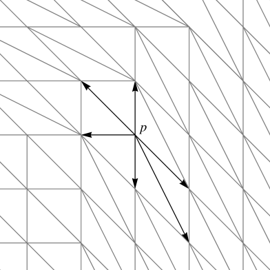
Our numerical scheme, Anisotropic Diffusion using Lattice Basis Reduction (AD-LBR), involves the construction of stencils whose geometry is tailored after the local diffusion tensor. Its essential feature is non-negativity: the discrete energy is written as a sum (3) of squared differences of values of , with non-negative weights . This discretization is consistent if for each , and any smooth ,
| (4) |
Indeed, the left hand side approximates the contribution of the “voxel” to the integral (1), while the right hand side is obtained by inserting the first order approximation in (3). The identity (4) is in turn equivalent to
| (5) |
The next lemma shows how to obtain such a decomposition in 2D. We denote by the rotation of a vector by , in such way that for all :
Lemma 1.
Let be such that , and . Then for any , with the convention :
| (6) |
Proof.
Note that . Denoting by the right hand side of (6), we obtain
Thus . Likewise , and . Since is a basis of , the result follows. ∎
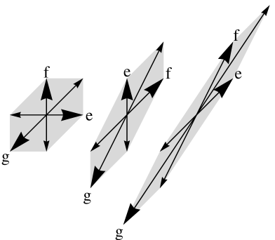
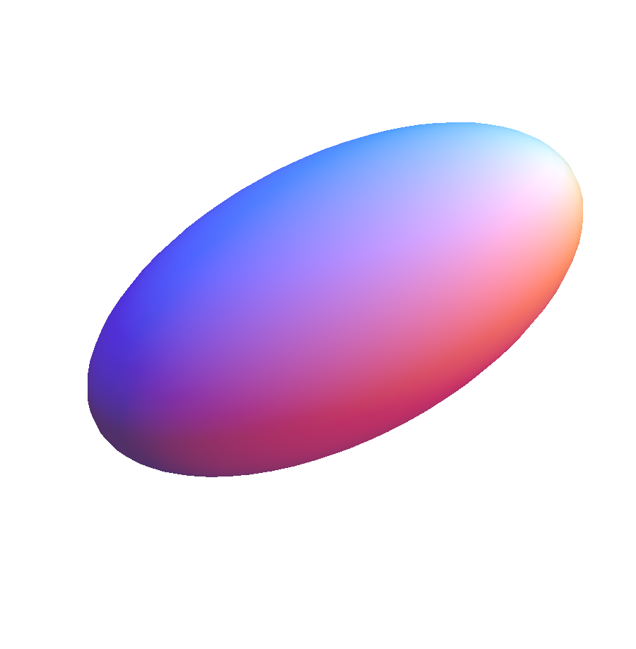
The diffusion tensor is meant to measure gradients, as in (1). In order to measure angles between vectors, we introduce a Riemannian metric 333The Laplace Beltrami operator associated to does not coincide with , unless is identically of determinant . This is not an issue for our application. on the domain , which is proportional to the inverse of : for all
| (7) |
The normalizing factor was chosen so as to normalize the metric determinant: . This normalization reflects the fact that the construction of our stencil depends on the preferred direction of diffusion, and on the amount of anisotropy, whereas the absolute strength of diffusion is irrelevant. In dimension , one easily checks that for any and any , one has
| (8) |
The AD-LBR is based on decompositions (5), given by the previous lemma, with a family of vectors chosen so that the scalar products appearing in (6) are non-positive. The adequate concept is that of -obtuse superbase of [4].
Definition 1.
-
•
A basis of is a family of elements of such that .
-
•
A superbase of is a family such that , and is a basis of .
Definition 2.
Let . A family of vectors in is said to be -obtuse if for all distinct .
In dimension , there exists for each at least one -obtuse superbase of [4]. The practical construction of such superbases is discussed in §2, and based on lattice basis reduction algorithms described in [11, 23, 17] (hence the name of our numerical scheme). This construction has a logarithmic numerical cost in the anisotropy ratio of the matrix :
| (9) |
The AD-LBR energy , see (3), is in two dimensions written in terms of the following stencils and coefficients. Let , and let be an -obtuse superbase of . We set
| (10) |
and for , with the convention ,
| (11) |
Lemma 1 implies the announced decomposition (5), and the weights are non-negative in view of (8). These weights , extended by outside , do not depend on the choice of -obtuse superbase , see Lemma 11. Stencils of the three dimensional AD-LBR are described in §2, and involve a construction of Selling444The authors would like to thank Professor P. Q. Nguyen for pointing out this points 3D stencil, which is simpler and sparser than the points stencil proposed by the authors in an earlier version of the manuscript. [22]. The above description of the stencils is suitable for periodic, reflected, and Dirichlet boundary conditions (extending by zero outside in the latter case). In the case of Neumann boundary conditions, a slight modification is in order:
We have so far established three strongpoints of the AD-LBR:
- Non-negativity.
-
Off diagonal coefficients of the symmetric semi-definite matrix, , associated to the energy are non-positive, while diagonal coefficients are positive.
- Sparsity.
-
Stencil cardinality is uniformly bounded, without restriction on the anisotropy ratio of the diffusion tensor.
- Complexity.
-
The construction of the stencil , and of the associated coefficients , has a logarithmic cost in the anisotropy ratio of the diffusion tensor.
The next result, Theorem 1, restricted to the two dimensional case, establishes that AD-LBR is asymptotically equivalent to a more involved and computationally intensive procedure: a finite element discretization of the energy (1), on an Anisotropic Delaunay Triangulation (ADT, see [10] and below) of the domain . Under the assumptions of Theorem 1, AD-LBR benefits from two additional guarantees, that we state informally and without proof.
- No chessboard artifacts.
-
Some numerical schemes for anisotropic diffusion suffer from chessboard artifacts, in the sense that periodic artifacts develop at the pixel level. Such artifacts cannot develop in finite element discretizations, since they would lead to high frequency oscillations of the finite element interpolant, and therefore to an increase of the energy (12). The asymptotic equivalence of the AD-LBR with a finite element discretization also rules out these defects.
- Spectral correctness.
-
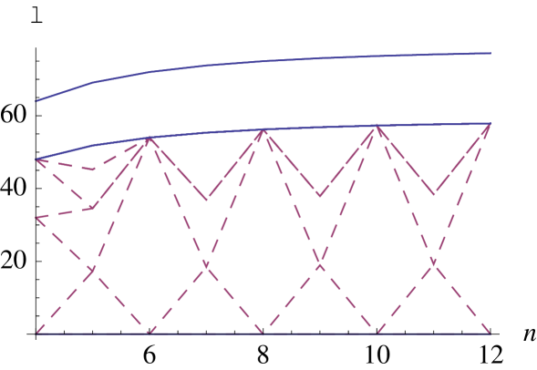
The -th smallest eigenvalue of the symmetric matrix associated to (3), converges as towards the -th smallest eigenvalue of the continuous operator , for any given integer . See Figure 8 page 8 for an illustration. This follows from a similar property of the finite element energy (12), and from the asymptotic equivalence (13).
Our convergence result, Theorem 1 below, is specialized to the case of a square periodic domain, which covers reflecting boundary conditions frequently used in image processing. Since the grid discretization must be compatible with the boundary conditions, any scale parameter appearing in the rest of the paper is assumed to be the inverse of a positive integer:
Theorem 1.
Let be the unit square , equipped with periodic boundary conditions. Let be a (periodic) diffusion tensor with Lipschitz regularity, and let be the Riemannian metric defined by (7). When is sufficiently small, the periodic Riemannian domain admits an Anisotropic Delaunay Triangulation , with collection of vertices . For , define
| (12) |
where denotes the piecewise linear interpolation operator on a triangulation . Then for some constant , independent of and ,
| (13) |
Let us mention that the finite element discretization on an ADT is a more general procedure than AD-LBR, since it does not require the domain to be sampled on a grid. This flexibility can be used to locally increase the density of vertices, in places where solution is expected to be less regular, or to insert vertices exactly on for a better discretization of boundary conditions. (Such refinements are however generally incompatible with image processing since the unknowns, the pixel values, lie by construction on a fixed and given cartesian grid.) Here and as often, the performance of AD-LBR is at the cost of its specialization.
The proof of Theorem 1 is postponed to §3, but for the sake of concreteness, we describe here the concept of Anisotropic Delaunay Triangulation (ADT) [10]. In the rest of this introduction, and in §3, we assume as in Theorem 1 that the diffusion tensor is defined on the square and satisfies periodic boundary conditions. We extend it, as well as the metric , to the whole plane by periodicity.
We specialize the concept of ADT [10], to the domain and the collection of vertices . For that purpose, we introduce some notations. For all , we denote by the distance from to , as measured by the metric at the point :
| (14) |
We denote by the least distance from a point , to the grid :
| (15) |
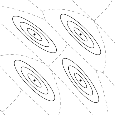
We introduce the Voronoi cell of a grid point , which is the collection of points closer to than to any other grid point:
| (16) |
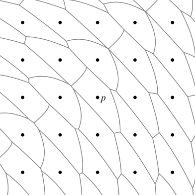
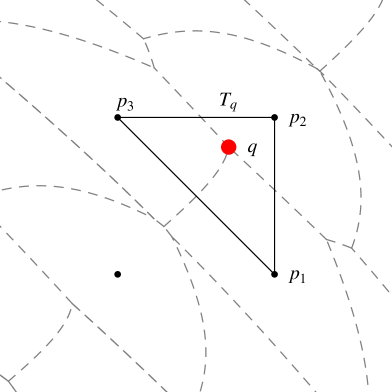
The collection of Voronoi cells is referred to as the Voronoi diagram, see Figure 2. A Voronoi vertex is a point at which at least three distinct Voronoi regions intersect: , , . We attach to a dual Voronoi cell , defined as the convex hull of the points , see Figure 3.
The geometric dual , of the Voronoi diagram, is defined as the collection of all dual Voronoi cells . Note that, generically on the metric , no more than three Voronoi regions can intersect at any point in , thus the elements of are generically triangles. If is small enough, we show in §3 (using the Dual Triangulation Theorem in [10]) that is a strictly convex polygon, of vertices with the above notations, and that is a polygonization (generically a triangulation) of , with vertices .
Since the metric and the vertices are periodic (recall that for some integer ), arbitrarily triangulating the elements of , respecting periodicity, yields a periodic triangulation .
Definition 3 (ADT, Labelle and Shewchuk [10]).
The triangulation obtained by the above construction is referred to as an ADT of the domain , with collection of vertices , and underlying Riemannian metric . Since is -periodic, we also regard it as an ADT of the periodic unit square .
We establish in §3.1 the existence of the ADT . Incidentally, we show in Lemma 7 (iii) page 7 that the angles of the elements of , measured with respect to the local metric , are asymptotically acute. This geometrical property (which holds thanks to our special choice of triangulation vertices, on a grid) is linked to the non-negativity of AD-LBR: indeed, it is known that finite elements discretizations such as (12) yield non-negative numerical schemes, and the discrete maximum principle, if the mesh satisfies a non-obtuse angle condition, see Lemma 3.1 in [9].
Subsection §3.2 is devoted to the study of -obtuse superbases of , and their cousins -reduced bases of , on which the AD-LBR relies: we discuss their characterization, uniqueness and stability properties. We study in §3.3 the finite element stencils, defined for by
| (17) |
see Figure 3 (right). We show that coincides with the AD-LBR stencil , unless the lattice admits a basis almost orthogonal with respect to the scalar product associated to , see Lemma 13. This is tied to the fact that orthogonal grids admit several (usual) Delaunay triangulations. Overcoming this technical difficulty, we conclude the proof of Theorem 1.
Note that the construction of the ADT is not easy to parallelize, in particular when anisotropy is pronounced since the Voronoi regions of far away points interact. The construction of also involves solving polynomial equations of degree four, because Voronoi regions boundaries are conics, and Voronoi vertices must be identified at their intersections. In contrast, the AD-LBR stencils are independent of each other, and the numerical cost of their construction only grows logarithmically with the metric anisotropy.
2 Construction of obtuse superbases, and three dimensional stencils
 |
|
 |
|
Algorithms for the construction of privileged bases of lattices, consisting of short and almost orthogonal vectors, have attracted an important research effort from the mathematical community, over a long period of time. The first such algorithm dates back to Lagrange [11], and is restricted to two dimensional lattices. Methods for high dimensional lattices, such as the LLL algorithm [12], are of key importance for integer programming and cryptography [18]. AD-LBR is based on the original algorithm of Lagrange [11], and on its recent extension to three dimensional lattices [23, 17]. These methods output a basis of reduced in the sense of Minkowski, which in dimension is equivalent to the following definition.
We denote by the sub-lattice of generated by vectors . This sub-lattice equals by convention if .
Definition 4.
An -reduced basis of , where and , is a basis of such that
| (18) |
For each , and each , there exists at least one -reduced basis [17]. In contrast, there exists for which no basis of satisfies (18). The norms of the elements of an -reduced basis,
| (19) |
are called the Minkowski minima, and are independent of the choice of -reduced basis. In particular, is the shortest vector of , with respect to the norm , and is the shortest linearly independent vector.
Lemma 2.
For any , ,
Proof.
Note that , for any . In addition: (i) any satisfies , and (ii) the set appearing in (18) always contains at least one element of the canonical basis of , so that . The announced result easily follows. ∎
We emphasize that obtaining an -reduced basis, i.e. solving the minimization problems (18), is both simple and cheap numerically. In dimension , this is the object of Lagrange’s algorithm [11] (later rediscovered by Gauss and often erroneously called Gauss’s algorithm, see [17]): initialize as the canonical basis of , and
| (20) | ||||
This algorithm can be regarded as a two dimensional geometrical generalization of greatest common divisor computation. It can be extended to higher dimension and, in dimension up to four, outputs an -reduced basis after at most iterations [17], each consisting of operations among reals.
The elements of an -reduced basis are heuristically never very far from being orthogonal, as illustrated by the following lemma.
Lemma 3.
Let , , and let be an -reduced basis. Then for any ,
| (21) |
Proof.
Since is an increasing function of , we may assume that . If follows from (18) that , and . Squaring these inequalities, and developing the scalar products, we obtain the announced result. ∎
Corollary 1.
Let , and let be an -reduced basis such that . Then is an -obtuse superbase of , with . In addition
| (22) |
Proof.
The previous Lemma implies Likewise . The result follows. ∎
The practical construction of the two dimensional AD-LBR stencil at a point amounts to (i) compute an -reduced basis using Lagrange’s algorithm (20), (ii) replace with , if necessary, so that , and (iii) define the stencil and the weights in terms of the -obtuse superbase of , where , as described in (10) and (11).
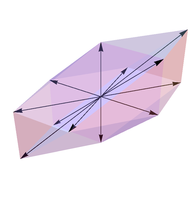
The rest of this section is devoted to the description of the three dimensional AD-LBR stencils. In constrast with the two dimensional case, the construction of the 3D stencil at a point , involves a -obtuse basis, instead of an -obtuse basis.
Proposition 1.
Let , and let be a -reduced basis. Let , for all , where the signs , and the permutation of are chosen so that
| (23) |
Then the following is a -obtuse superbase:
| (24) |
Proof.
To achieve (23), one can choose such that satisfies . Then choose the signs such that satisfies and .
The two families of vectors appearing in (24) are clearly superbases. We thus only need to show that they are -obtuse; in other words that for any two distinct elements of these families. Note that for all distinct , using (21),
In the case where , the pairwise scalar products between are non-positive by construction. In addition
Likewise for all , which concludes the proof.
We next turn to the second case, where . Enumerating all scalar products we obtain
and finally
This concludes the proof. ∎
In view of the previous Proposition, obtaining a -obtuse superbase of has numerical cost . Indeed a -reduced basis needs to be computed in a preliminary step, after what Proposition 1 is applied for a negligible cost. An alternative method for the construction of -obtuse superbases of is presented in [4] and in appendix B of [3], but its numerical complexity is not known to the authors.
The three dimensional AD-LBR is defined by the following stencils and coefficients. Let , let , and let be a -obtuse superbase of . We set
and if , and , then
As announced, , and the weights are non-negative. The proof of the scheme consistency (5), due to Selling [22], is reproduced in the next lemma for completeness. A generalization, appearing in Appendix B of [3], allows in arbitrary dimension to build a non-negative decomposition of the form (25) from a -obtuse superbase of . However the non existence of such a superbase, for some matrices , forbids a straightforward extension of AD-LBR to higher dimension.
Lemma 4 (Selling [22]).
Let be a superbase of . For all such that , , and , let . Then, for any :
| (25) |
Proof.
Let be as in the definition of . Then
since is a basis of . Also
In addition, clearly, Denoting by the right hand side of (25), we obtain as a result
Likewise for all . It follows as announced that . ∎
3 Equivalence to a finite element discretization
This section is devoted to the proof of Theorem 1: the asymptotic equivalence of AD-LBR with a finite element discretization on an Anisotropic Delaunay Triangulation (ADT). We use the notations of §1. The existence of the ADT is established in the first subsection, for sufficiently small, as well as a few of its properties. The second subsection is devoted to the study of -reduced bases. Theorem 1 is proved in the third subsection, by comparing the stencils of the AD-LBR and of the finite element discretization.
We denote by the maximum anisotropy ratio (9) of the diffusion tensor
| (26) |
Observing that , and recalling that , one easily checks that
| (27) |
for all and all .
3.1 Existence of an ADT
Our first lemma provides an uniform bound on the size of the Voronoi regions, see Figure 3, involved in the construction of the ADT.
Lemma 5.
-
(i)
For all , one has .
-
(ii)
If , and , then and .
Proof.
Point (i). Rounding the coordinates of to a nearest multiple of , we obtain a point such that . Recalling (27) we obtain , and therefore in view of (15).
Point (ii). We have . Thus , and likewise . Finally, by the triangle inequality, . ∎
Following the notations of [10], we denote by , , the smallest constant such that
Equivalently, in the sense of symmetric matrices,
| (28) |
We also define a quantity , closely related to the modulus of continuity of the metric :
| (29) |
One has as , for any continuous metric (indeed is periodic and therefore uniformly continuous). If is Lipschitz, as assumed in Theorem 1, then .
We show in the next lemma the existence of an ADT, by applying the main result of [10], under the assumption that is sufficiently small. More precisely, we assume in the rest of this subsection that
| (30) |
Lemma 6.
-
(i)
If , , and , then
-
(ii)
The geometric dual of the Voronoi diagram is, as announced in §1, a polygonization of into strictly convex polygons, with vertices .
Proof.
Point (i). We may assume that , otherwise there is nothing to prove. Point (ii) of Lemma 5 implies that , thus
On the other hand , and . The announced inequality follows.
Point (ii). We apply Theorem 7 (Dual Triangulation Theorem) in [10]. Since the domain has no boundary, it suffices to check that all the Voronoi arcs and vertices are wedged, see [10]. This condition means that for any such that , and any , one has , and likewise exchanging the roles of and . Heuristically, it expresses the acuteness of some angles measured in the local metric. Lemma 5 in [10] shows that this condition follows from point (i) of this lemma, which concludes the proof. ∎
We recall that is the triangulation obtained by arbitrarily triangulating the polygonization of the previous lemma, respecting periodicity, see Definition 3. Generically is already a triangulation, hence , see §1. The Voronoi regions , and the triangulation , are illustrated in Figures 2 and 3.
The next lemma provides estimates of the diameter, the area, and the angles of the elements of . These geometrical properties also have an interpretation in the context of lattices: (ii) shows that the edges of any triangle define a superbase of , and (iii) that this superbase is almost -obtuse, for any .
Note that the vertices of any triangle satisfy by construction
| (31) |
Lemma 7.
Denote by the edges of a triangle , where are oriented so that . Then
-
(i)
.
-
(ii)
, thus .
-
(iii)
, for any , where as . (Explicitly: )
Proof.
Point (i). We denote by the vertices of , ordered in such way that , , . The announced estimate follows from (31), and from point (ii) of Lemma 5.
Point (ii). Since is a conforming triangulation, the intersection of with the collection of all vertices of consists of only three points: the vertices of . Thus the triangle of vertices , homothetic to , contains no point of integer coordinates but its vertices. This implies that is a basis of , hence , as announced.
Point (iii). The pairwise distances between are bounded by , see point (i), and since so are the pairwise distances between . Defining , and observing that , we find that the pairwise distances between are bounded by .
Let . We have , thus
| (32) |
(For intuition: in a classical Delaunay triangulation, would be the circumcenter of , and (32) would state that is outside the circumcircle of .) Denoting , and , we obtain
| (33) |
using Lemma 5, and likewise for . We also have
Thus, proceeding as in (33),
Inserting in (32) these estimates of , , and using the fact that , see Lemma 5, we obtain after expansion the announced estimate of . ∎
We next rewrite the finite element energy (12) in a form similar to that of the AD-LBR energy (3). Let be the piecewise linear function on such that , and for any vertex distinct from . This is the classical “hat function” encountered in finite element analysis. For all , , let
| (34) |
Clearly, if is not an edge of , in other words if does not belong to the stencil , defined in (17). We express in the next lemma the finite element energy (12) in terms of the stencils and of the (potentially negative) weights .
Lemma 8.
For any , extended by periodicity to , one has
| (35) |
Proof.
For any triangle , and any , we denote
Clearly if or is not a vertex of . The coefficient , , is thus given by the following sum with at most two non-zero terms:
| (36) |
Let be the vertices of a triangle . Since the sum is constant on , equal to , it has a null gradient on , and therefore
Using this relation, and the two similar ones obtained by a cyclic permutation of , we obtain
Summing this expression over all , and combining it with (36), we obtain (35), which concludes the proof. ∎
Finally, we provide an approximation of the coefficients which will be easily compared with the AD-LBR weights (11).
Lemma 9.
Consider an edge of , shared by the two distinct triangles . Let (resp. ) be the two other vector edges of (resp. ), oriented so that (resp. ). Then
where .
Proof.
We assume, up to exchanging and , that is an edge of . Let , see point (ii) of Lemma 7; note that . Let be the constant value of on . Then and . These two independent linear identities are also satisfied by , hence on .
3.2 Some properties of -reduced bases
We establish some technical properties of -reduced bases, thanks to which we will be able to compare in §3.3 the “geometric” construction of the ADT finite element stencils , with the lattice based construction of the AD-LBR stencils .
Lemma 10.
Let , let , , and let . Assume that for all , with the convention :
| (37) | ||||
| (38) |
Then any -reduced basis satisfies
Proof.
Let . Our objective is to show that cannot be an element of an -reduced basis, and we may therefore assume that has co-prime coordinates.
It follows from (37) that the closed polygonal line of consecutive vertices , circles at least once around the origin, see Figure 5. Hence , for some and some . Since is a basis of (indeed ), the coefficients and are integers. Since , . Since has co-prime coordinates, .
Assuming without loss of generality that , we obtain using (38):
Observing that for all , we obtain . Since and are linearly independent, we have . Finally , hence cannot be an element of an -reduced basis, which concludes the proof. ∎
The next corollary reverses the construction, presented in Corollary 1, of an -obtuse superbase from an -reduced basis.
Corollary 2.
Let and let be an -obtuse superbase of , ordered so that . Then is an -reduced basis.
Proof.
The family satisfies by construction the conditions of the previous lemma. Hence any -reduced basis of satisfies . Observing that and are linearly independent, that , and that , we obtain that and . Recalling that -reduced bases are defined by the minimality of their -norms, see Definition 4, we obtain as announced that is an -reduced basis. ∎
The previous lemma shows that for any , there exists an -reduced basis such that
| (39) |


Given , and an -reduced basis of , we denote . This value can be expressed in terms of the Minkowski minima (19) and thus does not depend on the particular choice of -reduced basis. Indeed, recalling the identity
we obtain
| (40) |
In addition one has
| (41) |
where the right hand side follows from Lemma 3. A vanishing value, , indicates that the lattice admits an -orthogonal basis. In contrast, when the upper bound is met, , one has for , hence the reduced basis is not unique even up to sign changes. See Figure 5.
We next show that the stencils of the AD-LBR do not depend on the choices of reduced bases, as was announced in the introduction.
Lemma 11.
The weights used in the AD-LBR at a point (defined on by (11) and extended to by ), do not depend on the choice of -obtuse superbase of .
Proof.
We denote and . Let and be two -obtuse superbases, and let and be the corresponding AD-LBR stencils and weights defined by (10) and (11). We may assume, using Corollary 2 and up to reordering, that and are -reduced bases.
Corollary 1 states that the scalar products , , and are (strictly) negative. On the other hand
| (42) |
The next lemma establishes weak uniqueness and stability properties for -reduced bases, in the case of a strict inequality
Lemma 12.
Consider , an -reduced basis , and an -reduced basis . Let be such that , in the sense of symmetric matrices. Assume either:
-
(i)
, and (i.e. ).
-
(ii)
, and .
Then
3.3 Comparison of the stencils
We assume in this subsection that the scale parameter is sufficiently small. Our assumption is stronger than the one used in §3.1, see (30), hence in particular there exists an Anisotropic Delaunay Triangulation . More precisely we assume that
| (45) |
See (26), (29), and Lemma 7 for the definition of , and respectively. For Lipschitz metrics, and .
Our objective is to compare the stencils , , of the AD-LBR (10) and of the ADT finite element discretization (17) respectively, at a point . The next lemma shows that they are equal unless the lattice is almost orthogonal with respect to the local metric; a property quantified via , see (40).
Lemma 13.
Let , and let . If , then . In any case, one has for any -reduced basis :
| (46) | ||||
| (47) |
Proof.
We assume that , up to replacing with . Let be a triangle containing , and let be the edges of , oriented so that . Using point (iii) of Lemma 7, and (27), we obtain for all , with the convention
| (48) |
Denote , and . Applying Lemma 10 to and the points , we obtain that . Up to exchanging with , we thus have or . Since the elements of sum to zero, we conclude that
| (49) |
which implies (47).
Let be a triangle containing and intersecting the half line . We know (49) that is a vector edge of (i.e. the difference between two vertices of ). The corresponding edge segment must be , since otherwise would be empty. Thus . Applying the same argument to , we obtain (46).
If , then is also a vector edge of any triangle containing , since we eliminated the second case in (49). Reasoning as above we find that , and therefore . Thus . This concludes the proof. ∎
We introduce new stencils , for , defined as follows. Let . If , then denoting by an -reduced basis,
| (50) | ||||
| (51) |
On the other hand, if , then
| (52) |
The previous lemma implies that for any .
Lemma 14.
The stencils , , do not depend on the choice of -reduced basis.
Proof.
Let be the energies associated to the stencils : for , extended to by periodicity,
The outline of the proof of Theorem 1 is as follows. We prove in Lemmas 16, 17 and 15 respectively that for any :
| (53) | ||||
| (54) | ||||
| (55) |
where the constants only depend on the metric . Combining these inequalities, and recalling that and for Lipschitz metrics ( is defined in Lemma 9), we obtain
for some constant . This establishes (13), and concludes the proof of Theorem 1.
For each , we denote by , , the characteristic functions of and respectively. The proofs of (53) and (55) immediately result from the comparison, in Lemmas 16 and 15 respectively, of the coefficients , , , appearing in the expressions of .
In the following, it will be convenient to express the AD-LBR weights, and others, in terms of the scalar product associated to the Riemannian metric. We thus recall (8): for any , and any ,
We also define the bounds ()
Lemma 15.
For any , one has on
Proof.
Let , and let be an -obtuse superbase of . We can assume, thanks to Corollary 2, that is an -reduced basis. Then using (22)
hence , and likewise . If , then , and this concludes the proof.
Assume now that . Then
hence . The result follows since . ∎
Let and let be the consecutive elements of , in trigonometric order. We define for all , denoting ,
with the periodic conventions , . We also set on .
Lemma 16.
Proof.
The coefficients , , , are all equal to zero outside of . This holds by construction of , and by Lemma 13 for , . We may therefore forget about the presence of in (56).
First inequality. Lemma 9 states that on , which concludes the proof.
Second inequality. If , then . Comparing the definition of with that of (11) we observe that on , which concludes the proof in this case.
Assume now that . Let be an -obtuse superbase of . We can assume, thanks to Corollary 2 that is an -reduced basis. Looking at (11) and denoting , we find that
Likewise . In addition
Combining the definition of with the description of the stencil in Lemma 13, we obtain that
In any case . The expressions and estimates of at the points are obtained similarly. Likewise, using Lemma 13,
In any case . The expressions and estimates of at the points are similar. Comparing the above estimates of , , we obtain that on . Since , this concludes the proof. ∎
In the last lemma of this section, we control the contribution to the energy of a stencil , , in terms of the contributions to of and of the neighboring stencils , . This leads to an estimate of in terms of , which concludes the proof of Theorem 1.
Lemma 17.
One has , for any , with .
Proof.
Consider a grid point , and denote . Assume first that , so that . Consider also an arbitrary , and observe that for some -reduced basis .
4 Numerical experiments
We compare our scheme AD-LBR with a family of other schemes: finite difference, finite elements, and two schemes from the image processing literature. We begin with a quantitative comparison for the discretization of the restoration equation, in a synthetic case where the exact solution is analytically available for reference. The second test case is a qualitative comparison of Coherence-Enhancing Diffusion (CED) [25], on a real image and the quality assessment is by visual inspection. Finally we present a 3D implementation of AD-LBR for proof of feasibility, featuring a synthetic CED experiment, and a application of Edge Enhancing Diffusion to MRI data.
4.1 The different schemes
Our two dimensional numerical experiments feature the following six numerical schemes for anisotropic diffusion.
-
➣
AD-LBR: the scheme presented in this work.
- ➣
-
➣
Bilinear Finite Elements (Q1). Bilinear finite elements, also referred to as Q1 finite elements, are linear with respect to each space direction. This amounts to use a 9 points stencil, where the coefficients are different from the previous scheme.
-
➣
Weickert-Scharr scheme (WS). This scheme, introduced in [27], is based on a second order approximation of the gradient using a centered stencil. As a result, it offers good accuracy and rotation invariance when applied to sufficiently smooth functions, but lacks robustness guarantees such as the discrete maximum principle and spectral correctness (see §1), even for . The stencil for this scheme has size .
- ➣
- ➣
Note that other schemes exist, see for instance [16, 28]. While an exhaustive comparison is in principle desirable, it could not be done here due to time and space constraints.
To fix the ideas and illustrate the difference between the schemes, we propose to compute the stencil and the coefficients for different constant diffusion tensors , in isotropic and anisotropic cases. Denoting by the matrix of rotation by the angle , and by the chosen anisotropy ratio, we set, identically on :
| (60) |
The results are presented in Tables 1 and 2. Note that for the two last cases (anisotropy and ) the AD-LBR stencil contains points that are outside the neighborhood of the pixel. However the stencil contains 6 points, as expected. This contrasts with the schemes FD, Q1, W-NN where only the neighborhood is involved. Another observation is that the off-center stencil coefficients of the AD-LBR are non-positive (this gives non-negative off-diagonal coefficients for ), in contrast with schemes FD, Q1, WS, and with scheme W-NN for anisotropy . This is an essential property of AD-LBR (and A-NN), and as a consequence our scheme satisfies, unconditionally, the discrete maximum principle [1, 6].
The largest eigenvalue of the discrete operator is given in Table 3, for the different schemes. It turns out that AD-LBR has in most cases the smallest eigenvalues among all schemes, except for scheme WS and occasionally A-NN. This property allows (although this was not done in our numerical experiments) to use larger time steps for AD-LBR than for the other schemes, when solving parabolic equations (2) or (64) with an explicit time discretization.
Operator splitting is a classical approach to further increase the timestep in (potentially anisotropic and non-linear) diffusion PDEs [25, 26, 2]. The AD-LBR is compatible with Additive Operator Splitting, by applying Remark (e) page 111 in [25], although the efficiency of this technique is here compromised by the potentially large number of directions in our adaptive stencils. Let us also mention Multiplicative Operator Splittings, and Additive-Multiplicative Operator Splittings, which allow to combine different time-steps [2, 8]. None of these methods was used in our experiments.
Remark 1 (Axes-directed non negative six point scheme).
The following six point scheme A-NN is, in our belief, the best possible implementation of the constructive proof in [25] of the existence of non-negative schemes for two dimensional anisotropic diffusion. Like AD-LBR, this scheme is defined by the data at each point of a stencil , and of non-negative weights .
Let In the diagonal case , the scheme A-NN relies on the classical four points stencil. Otherwise note that
Let be such that ,
| (61) |
and is minimal. The scheme A-NN is defined by the six point stencil
and the non-negative weights
These coefficients are non-negative by construction, and consistency (5) is easily checked. Contrary to AD-LBR, the coordinate axes play a privileged role in A-NN. This introduces axis aligned artifacts which are visible in Figure 12 (g).
Remark 2 (Stencil radius).
The two dimensional stencils of AD-LBR coincide with those of FM-LBR, a numerical scheme for anisotropic static Hamilton-Jacobi PDEs introduced in [14] the second author. As shown in Proposition 1.6 of [14], the euclidean radius
of this stencil is bounded by .
In contrast, consider for the matrix
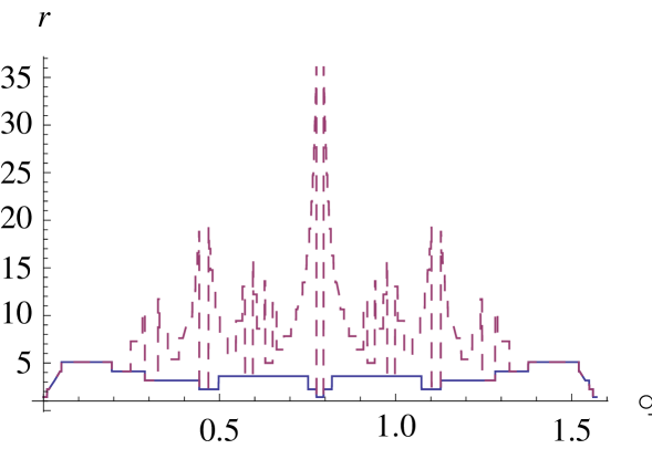
If follows from (61) that . From this point, one easily obtains that . The radius of the A-NN stencil, at a point , may thus be of the order of . The radii of the AD-LBR and A-NN stencils, computed for diffusion tensors of anisotropy and of various orientations, are illustrated on Figure 7.
 |
Remark 3 (Scheme FD).
The operator is discretized using centered finite differences [15]. This involves quantities defined at half integer indices, and in particular the diffusion tensor is here given on the offsetted grid , . For the sake of readability, we thus define and . The gradient operator is discretized by:
The divergence is defined as follows:
with
and similar terms involving .
| () | ||
|---|---|---|
| stencil for AD-LBR | ||
| stencil for FD | ||
| stencil for Q1 | ||
| stencil for WS | ||
| stencil for W-NN | ||
| stencil for A-NN |
| stencil for AD-LBR | ||
|---|---|---|
| stencil for FD | ||
| stencil for Q1 | ||
| stencil for WS | ||
| stencil for W-NN | ||
| stencil for A-NN | ||
| eigenvalue AD-LBR | 8 | 4.27 | 2.06 | 1.06 |
|---|---|---|---|---|
| eigenvalue FD | 8 | 6.22 | 5.06 | 4.85 |
| eigenvalue Q1 | 5.7 | 4.94 | 4.32 | 4.20 |
| eigenvalue WS | 1 | 1 | 1 | 1 |
| eigenvalue W-NN | 8 | 4.27 | 3.1 | 3.02 |
| eigenvalue A-NN | 8 | 4.27 | 1.04 | 0.3 |
4.2 A test case with an explicit solution
Consider an image , defined on a domain , and a diffusion tensor field . A classical approach to restore the image , if it has been corrupted by additive noise, is to find which minimizes:
| (62) |
In other words, is a penalized least squares approximation of . The parameter should be adjusted so as to avoid excessive smoothing (for large ), or insufficient denoising (for small ). The solution can be characterized as the solution to the static elliptic PDE:
| (63) |
In applications [20, 24] the diffusion tensor is usually adapted to the local image structure, in order to avoid smoothing the edges of . We construct below a test case (image and tensor field ), for which the solution is known analytically.
In order to obtain an analytic solution, we first consider a separable problem where the image is invariant by translation along the horizontal axis, and the metric is constant with axes parallel to the coordinate axes. This first problem is invariant under translations along the -axis, and therefore boils down to a 1-dimensional problem. This separable problem is then transported by a diffeomorphism in order to obtain a new problem where the axes of the metric are no more parallel to the coordinate axes.
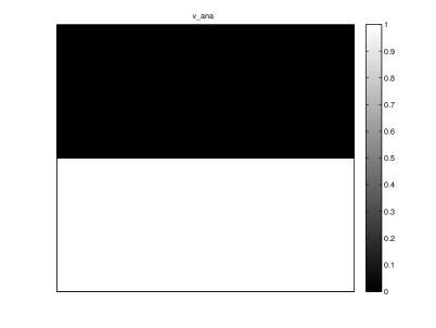
The analytical image is composed of a black and a white stripe: , see Figure 9. Given , we consider the constant diffusion tensor
The analytical solution of (63), applied to and , is known in the case of the infinite domain . In Fourier domain all the coefficients are real and:
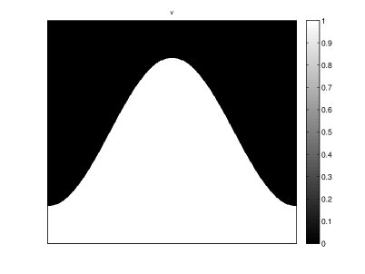
This separable problem is transformed using the following diffeomorphism: for
The Jacobian of is
We apply the different restoration schemes to the image , and the following diffusion tensor:
where we denoted and . The numerical solution is compared to the analytical function , which is the exact solution in the case of the infinite domain . This numerical solution was obtained on the bounded domain , equipped with reflecting boundary conditions. Numerical evidence suggests that this change of domain and of boundary conditions has only an anecdotic impact on the solution of (63), with the parameters chosen in this test case.
We used in the numerical experiments. The maximum value of , among all , is equivalent to .
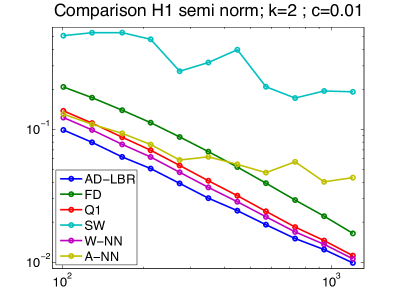
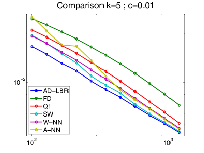
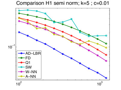
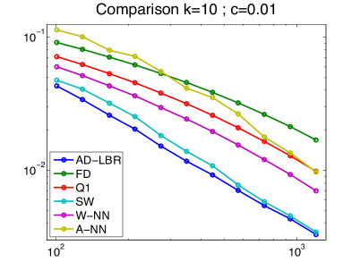
4.3 Results for the synthetic test case
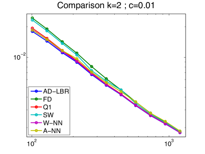
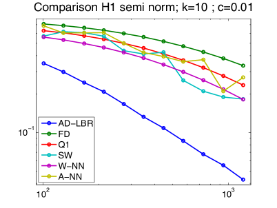
We present in Figure 10 the performance results of the different schemes, for different values of the anisotropy , obtained on a series of grids of size ranging from to . The anisotropy varies from to , which are relevant values for imaging applications, see the numerical experiments in §4.4. The quality of a scheme is measured by the difference and the semi-norm difference between the numerical solution and the analytical solution. Note that the error is concentrated close to the discontinuity, since the solution tends rapidly to a constant (0 or 1) far from the discontinuity. We chose the smoothing parameter in (62). The linear equation obtained by the discretization of (63) is solved using Conjugate Gradient.
We also tested extreme anisotropies, (thus ), which can be relevant in physics related applications. None of the tested schemes showed convincing results: methods based on fixed stencils fail because the discrete operator looses positivity, while the AD-LBR (and A-NN even more) suffers from under-sampling due to the large radius of its stencils. We thus refer to [7] for a radically different approach tailored for this setting. This method introduces an auxiliary one-dimensional unknown, which is constant on the field lines (obtained in a preprocessing step) of the anisotropy direction field, and varies orthogonally to them.
The performance advantage of the AD-LBR is particularly clear when the error is measured in the semi-norm: for the anisotropy and the resolution , which are relevant values in image processing, AD-LBR outperforms its alternatives by a factor ranging from 3 to 5.
4.4 Coherence-enhancing diffusion
In order to document the interest of our discretization, we implement Coherence-Enhancing Diffusion [25] using the different numerical schemes at our disposal. The following parabolic equation is considered:
| (64) |
This equation is non-linear since the diffusion tensor depends on the solution . This tensor also depends on four user defined parameters , . Let (resp. ), be the Gaussian kernel of variance (resp. ). Define the convolution , and the structure tensor . The diffusion tensor possesses the same eigenvectors as , and if the eigenvalues of are then the eigenvalues of are
This ensures that one smoothes preferably along the coherence direction , with a diffusivity that increases with respect to the coherence . When the time parameter becomes large, the image tends to a constant image, therefore it is necessary to stop the process at some finite time . The ratio of the eigenvalues is bounded by , hence .
We used an explicit time discretization for (64), with time step . The image at time is defined by the explicit equation:
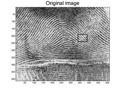
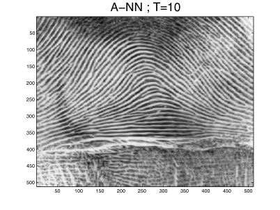
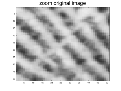
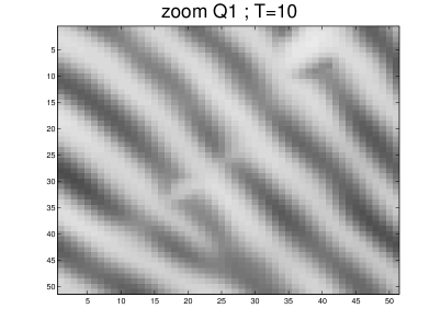
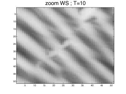
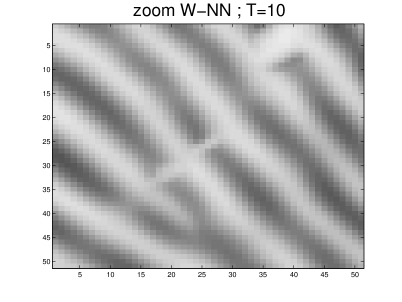
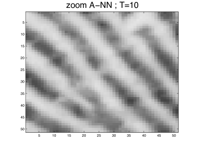
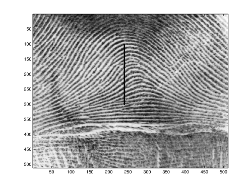
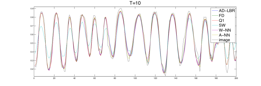
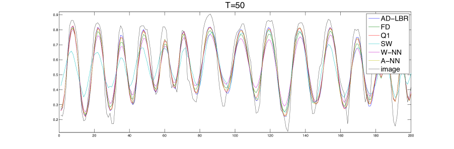
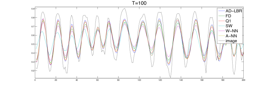
The parameters used in our simulation were: , , , and . This gives a maximum anisotropy of . The algorithm was applied to a fingerprint image. The results obtained for are shown in Figures 11 and 12, and they document the ability of our scheme to close interrupted lines more efficiently than the other schemes. The largest eigenvalue of the discrete operator at is given in Table 4 for the different schemes. As was already noticed in the constant metric case, it turns out that AD-LBR has the smallest eigenvalues among all schemes, except for scheme WS. This property allows (although this was not done in our numerical experiments) to use larger time steps for AD-LBR than for the other schemes.
Note also that ridges are clearer, and valleys are darker, using AD-LBR than with the other schemes. (Gray-scale range is the same for all images, see also Figure 13). This reflects the fact that AD-LBR avoids, better than the other schemes, smoothing transversally to the orientation encoded in the continuous anisotropic PDE (64).
Remark 4 (Computation time).
Numerical solvers of the parabolic PDE (64) combine three main components: (i) Constructing the diffusion tensor. (ii) Assembling the discretization stencils and the operator sparse matrix. (iii) Performing an explicit time step. Components (i) and (ii) are executed exactly the same number of times, while step (iii) is generally more frequent: in order to save CPU time, one typically does not update the diffusion operator at each time step. We produced a C++ implementation of AD-LBR, within the Insight Toolkit open source library. Although our code is neither parallel nor aggressively optimized, we believe that comparing the CPU times for steps (i), (ii) and (iii) is informative, and allows to estimate the additional cost of AD-LBR which is essentially contained in step (ii).
For our 2D Coherence-Enhancing Diffusion (CED) experiment, on the fingerprint image, (i) takes 0.21s, (ii) 0.027s, (iii) 0.005s. For our 3D CED Experiment, on synthetic data, (i) takes 1.35s, (ii) 0.51s, (iii) 0.035s. In both cases, the AD-LBR specific step (ii) is dominated by the construction of the diffusion tensor (i). Step (ii) may also be dominated by the mere cost (iii) of iterations, provided the operator is updated less than once every 6 explicit steps in 2D (14 in 3D). To our eyes, the limited additional cost (ii) of AD-LBR is acceptable in view of the strong theoretical guarantees, and qualitative improvements, brought by this scheme.
| scheme | AD-LBR | FD | Q1 | WS | W-NN | A-NN |
| eigenvalue | 3.75 | 5.67 | 5.09 | 0.96 | 3.83 | 6.23 |


4.5 3-dimensional experiments
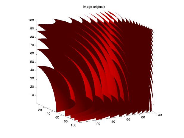
In order to illustrate the feasibility of our scheme in 3D space, we present the action of anisotropic diffusion PDEs on two examples. The first example is a 3D analog of the synthetic test case presented in [27], featuring Coherence-Enhancing Diffusion. The second one is the application of Edge-Enhancing Diffusion to a MRI scan.
Synthetic example
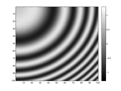
The original, radially varying image is defined on the cube . The gray-level at a point is defined by
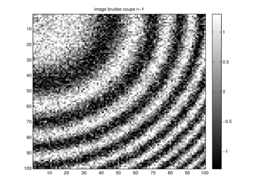
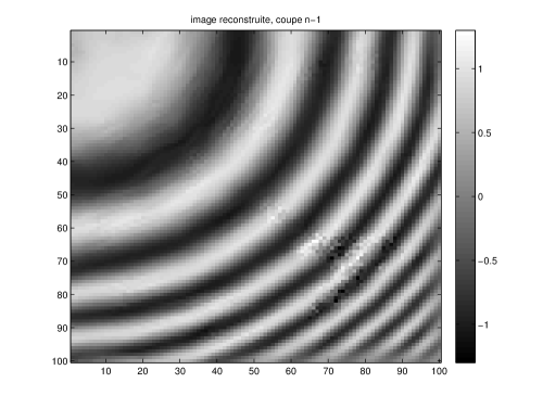
where and . This image presents a series of concentric level-sets. We present in Figure 14 the level sets , and a slice through the plane .
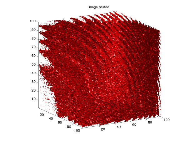
The image is perturbed by
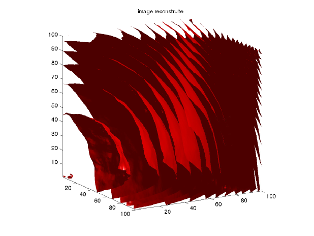
where is an additive Gaussian noise of variance . The reconstructed image is obtained using a 3D Coherence-Enhancing Diffusion PDE [25], similar to the 2D one in section 4.4:
where is the structure tensor defined by , . The tensor possesses the same eigenvectors as , and if the eigenvalues of are then the eigenvalues of are
where . The anisotropy ratio is bounded by . We used the values , . The problem is discretized using voxels. We present in Figure 14 the noisy image (levelset 0 and planar slice) and the result after 20 time-steps of .
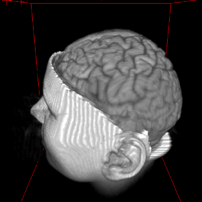
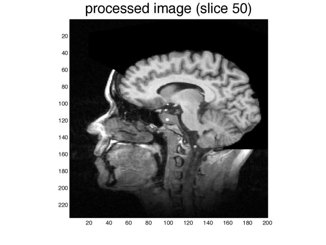
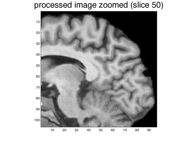
3D MRI data
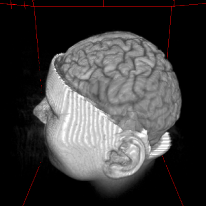
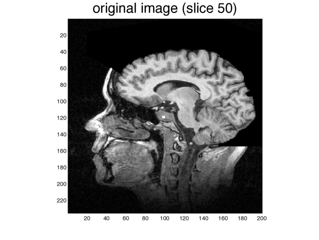
The data is a Magnetic Resonance Imaging scan of a skull, and was obtained from the ”University of North Carolina Volume Rendering Test Data Set” archive.
The reconstructed image is obtained using a 3D Edge-Enhancing Diffusion PDE [25], which differs from the above Coherence-Enhancing Diffusion one by the choice of the diffusion tensor eigenvalues. The optimal choice of these eigenvalues indeed depends on the application, and is still an active subject of research [13]. With the above notations, the eigenvalues of are
We used the values , . In our experiment, the maximum anisotropy ratio was . We present in Figure 15 the original image and two slices of the result after 10 time-steps of .

Conclusion
We introduced in this paper a new numerical scheme, AD-LBR, for anisotropic diffusion in image processing. This scheme is non-negative, and its stencils have a limited support: 6 points in 2D, 12 points in 3D. The former property implies that our scheme respects the maximum principle of Alvarez, Guichard, Lions and Morel, which is an essential feature of parabolic PDEs.
AD-LBR outperformed all tested alternatives in a quantitative numerical experiment: a test case in which approximate numerical solutions are compared against a known analytical solution. In a second qualitative test case, different schemes were used to enhance a fingerprint image. Our scheme appears here to close more efficiently the lines of the fingerprint, and to diffuse less orthogonally to the lines. This is precisely the purpose of the implemented PDE, coherence enhancing diffusion. We also presented a 3-dimensional implementation as a proof of feasibility.
The construction of the stencils of the AD-LBR is both original and non-trivial. The computational load for this aspect of the algorithm is fortunately not dominant, thanks to the use of a tool from discrete geometry: lattice basis reduction. The AD-LBR also allows to use larger time steps than most of its counterparts, in explicit discretizations of parabolic equations.
AD-LBR trivially extends to vector valued and matrix valued images, by applying it on each image component independently. (In other words, the coupling between image components lies in the construction of the common diffusion tensor , which AD-LBR regards as user input.) Future work will be devoted to the application of AD-LBR to the regularization of diffusion tensor fields, arising for instance from diffusion MRI, for which we expect it to be particularly appropriate: thanks to the scheme non-negativity, positive-definiteness is naturally preserved.
References
- [1] L. Alvarez, F. Guichard, P.-L. Lions, J.-M. Morel, Axioms and fundamental equations of Image processing, Arch. Rational Mech. Anal., vol. 123, 199–257 (1993)
- [2] D. Barash, T. Schlick, M. Israeli, and R. Kimmel, Multiplicative operator splittings in non-linear diffusion: from spatial splitting to multiplicative timesteps, Journal of Mathematical Imaging and Vision, 19:33-48, (2003).
- [3] J.-B. Bost and K. Künnemann, Hermitian vector bundles and extension groups on arithmetic schemes. I. Geometry of numbers, 2010
- [4] J. H. Conway, N. J. A. Sloane, Low-dimensional lattices. VI. Voronoi reduction of three-dimensional lattices., Proceedings of the Royal Society of London. Series A: Mathematical and Physical Sciences 436.1896 (1992): 55-68.
- [5] G.-H. Cottet, L. Germain, Image processing through reaction combined with nonlinear diffusion, Math. Comp., vol. 61, 659–673 (1993).
- [6] L. Dascal, A. Ditkowski, and N. Sochen, On the Discrete Maximum Principle for the Beltrami Color Flow, J. Math. Imaging Vision, vol. 29, 63–77 (2007)
- [7] P. Degond, A. Lozinski, J. Narski, C. Negulescu, An Asymptotic-Preserving method for highly anisotropic elliptic equations based on a micro-macro decomposition, J. Comput. Phys., vol. 231(7), 2724–2740 (2012)
- [8] S. Grewenig, J. Weickert, and A. Bruhn, From box filtering to fast explicit diffusion, Pattern Recognition 533-542, (2010).
- [9] W. Huang, Discrete maximum principle and a Delaunay-type mesh condition for linear finite element approximations of two-dimensional anisotropic diffusion problems, arXiv preprint arXiv:1008.0562, (2010)
- [10] F. Labelle, J. R. Shewchuk, Anisotropic Voronoi Diagrams and Guaranteed-Quality Anisotropic Mesh Generation, Proceedings of the Nineteenth Annual Symposium on Computational Geometry, 191-200 (2003)
- [11] J. L. Lagrange, Recherches d’arithmétique, Nouveaux Mémoires de l’Académie de Berlin, (1773)
- [12] A. K. Lenstra, H. W. Lenstra, and L. Lovász, Factoring polynomials with rational coefficients, Mathematische Annalen 261, 513–534, (1982)
- [13] A. M. Mendrik, E. J. Vonken, A. Rutten, M. A. Viergever, and B. van Ginneken, Noise reduction in computed tomography scans using 3-d anisotropic hybrid diffusion with continuous switch, Medical Imaging, IEEE Transactions on, 28(10), 1585-1594. (2009)
- [14] J.-M. Mirebeau, Anisotropic Fast Marching on Cartesian Grids, using Lattice Basis Reduction, preprint, 2012.
- [15] A. Mitchell and D. Griffiths The Finite Difference Method in Partial Differential Equations. Chichester: Wiley (1980).
- [16] P. Mrázek and M. Navara, Consistent positive directional splitting of anisotropic diffusion, Proc. Sixth Computer Vision Winter Workshop, (2001)
- [17] P. Q. Nguyen, and D. Stehlé, Low-dimensional lattice basis reduction revisited, ACM Transactions on Algorithms, Article 46 (2009).
- [18] P. Q. Nguyen and J. Stern, The two faces of lattices in cryptology, In Proceedings of the 2001 Cryptography and Lattices Conference (CALC’01). Lecture Notes in Computer Science, vol. 2146. Springer-Verlag, 146–180, (2001)
- [19] S. Osher, L. Rudin Feature-oriented image enhancement using shock filters, SIAM J. Numer. Anal., vol. 27, 919–940 (1990)
- [20] P. Perona and J. Malik, Scale-Space and Edge Detection Using Anisotropic Diffusion, IEEE Trans. Patt. Anal. Mach. Int., vol. 12, 629–639 (1990)
- [21] B. Schmid, J. Schindelin, A. Cardona, M. Longair, M. Heisenberg, A high-level 3D visualization API for Java and ImageJ. BMC Bioinformatics, 11:274 (2010)
- [22] E. Selling. über die binären und ternären quadratischen formen, J. reine angew. Math., 77:143–229, (1874).
- [23] I. Semaev, A 3-dimensional lattice reduction algorithm, In Proceedings of the 2001 Cryp- tography and Lattices Conference (CALC’01). Lecture Notes in Computer Science, vol. 2146. Springer-Verlag, 181–193, (2001)
- [24] J. Weickert, Theoretical foundations of anisotropic diffusion in image processing, Computing, SUppl. 11, 221–236 (1996)
- [25] J. Weickert, Anisotropic Diffusion in Image Processing, Teubner, Stuttgart (1998)
- [26] J. Weickert, B. Romeny, and M. Viergever, Efficient and reliable schemes for nonlinear diffusion filtering, IEEE Trans. Image Proc., vol. 7, 398–410 (1998)
- [27] J. Weickert, and H. Scharr, A scheme for coherence-enhancing diffusion filtering with optimized rotation invariance, J. Visual Comm. Image Rep., Vol. 13, 103–118, (2002).
- [28] M. Welk and G. Steidl and J. Weickert, Locally analytic schemes: A link between diffusion filtering and wavelet shrinkage, Applied and Computational Harmonic Analysis, 24, pp 195–224, (2008)