Sparse Quadratic Optimisation over the
Stiefel Manifold with Application to
Permutation Synchronisation

We start by ensuring that, under the assumption that $Z_{t}(U_{t})$ is full rank, the sequence $\{U_{t}\}$ generated by Algorithm 1 converges to the dominant subspace of $W$. This can straightforwardly be shown by using the following result.

Thus, if $Z_{t}(U_{t})$ is full rank for each $t$, we can identify our Algorithm 1 with Algorithm A in Lemma 3, and conclude that the sequence $\{U_{t}\}$ converges to the dominant subspace of $W$ as $t\rightarrow\infty$. This is because Algorithm B in Lemma 3 corresponds to the Orthogonal Iteration algorithm, which is known to converge to the dominant subspace of $W$ [21].

We continue by investigating the behaviour at the limit where the columns of $U_{t}$ are in the dominant subspace of $W$. Let us consider the update $U_{t+1}R_{t+1}\leftarrow WU_{t}Z(U_{t})$ of Algorithm 1, and further assume that the $d$ largest eigenvalues of $W$ are equal, which is for example the case for synchronisation problems assuming cycle consistency (cf. Sec. 4).

Hence, under the assumptions in Lemma 4, the columns of $U_{t^{\prime}}$ span the dominant subspace of $W$ for any $t^{\prime}\geq t$. The update in Algorithm 1 reduces to the form

i.e. updating $U_{t}$ to obtain $U_{t+1}$ simplifies to multiplication of $U_{t}$ with the $Q$-matrix from the QR-factorisation of $Z(U_{t})$.

We now turn our attention to the choice of $Z(U_{t})$ in Algorithm 1. We know that, as long as $Z(U_{t})$ is full rank in each iteration $t$, the columns of $U_{t}$ converge to the dominant subspace of $W$. In addition to our objective function $f$ in Problem (1), we now introduce the secondary objective

where for $p$ being a positive integer the notation $U.^{\wedge p}$ means to raise each element in $U$ to the power $p$. For $U\in\operatorname{St}(m,d)$ and $p$ larger than $2$, the maximisation of $g$ promotes sparsity in a relaxed sense. To be specific, if $p$ is odd, a few larger elements (with value close to 1) lead to a larger value of $g$ compared to many smaller elements (with value close to 0), so that sparsity and non-negativity are simultaneously promoted. Analogously, if $p$ is even, a few elements with value closer to $\pm 1$ lead to a larger value of $g$ compared to many smaller elements close to $0$.

Let us consider the maximisation of

with respect to $Q$, where $h(U,Q)=(UQ)^{T}((UQ).^{\wedge(p-1)}),$ $Q\in\mathbb{O}^{d}$, and $U\in\operatorname{St}(m,d)$. This means that we want to rotate $U$ by $Q$ in such a way that the secondary objective $g$ is maximised after the rotation. By applying the rotation from the right, we ensure that the columns $U$ span the same space after the rotation, but a higher objective value is achieved for the secondary objective $g$ in (4).

The extrinsic gradient with respect to $Q$ (for $Q$ relaxed to be in $\mathbb{R}^{d\times d}$) of $g(UQ)$ at $Q=\mathbf{I}$ is $p{\cdot}h(U,\mathbf{I})$. Thus the (manifold) gradient of $g(UQ)$ at $Q=\mathbf{I}$ is given by the projection of the extrinsic gradient at $Q=\mathbf{I}$ onto the tangent space, which reads

For a small step size $\alpha$, we can perform a first-order approximation of gradient ascent if we choose $Z=\mathbf{I}+\alpha p(h(U,\mathbf{I})-h^{T}(U,\mathbf{I}))$, and then update $U$ in terms of the Q-matrix of the QR-factorisation of $Z$. Now, let us assume that we investigate the behaviour at the limit under the assumptions in Lemma 4, i.e. that the $d$ largest eigenvalues of $W$ are equal. In this context the Q-matrix of the QR-factorisation is a retraction [3] and serves as a first-order approximation of the exponential map. With that, the updates become

This choice of the matrix $Z(U_{t})$ ensures that it is full rank, since adding the identity matrix and a skew-symmetric matrix results in a full rank matrix. Hence, for sufficiently small step size $\alpha$, we iteratively move in an ascent direction on $\mathbb{O}^{d}$ by utilising the QR-retraction.

Permutation synchronisation is a procedure to improve matchings between multiple objects [23, 34], and related concepts have been utilised to address diverse tasks, such as multi-alignment [7, 5, 25], multi-shape matching [22, 24, 20], multi-image matching [51, 42, 9, 13, 12], or multi-graph matching [48, 6, 41], among many others. Permutation synchronisation refers to the process of establishing cycle consistency in the set of pairwise permutation matrices that encode correspondences between points in multiple objects. In computer vision there is a typical application where the points are feature descriptors or key-points, and the objects are images, as shown in Fig. 2.

Let $k$ denote the number of objects, where each object $i$ contains $m_{i}$ points. For $\mathbf{1}_{p}$ being a $p$-dimensional vector of all ones, and vector inequalities being understood in an element-wise sense, let $P_{ij}\in\mathbb{P}_{m_{i}m_{j}}:=\{X\in\{0,1\}^{m_{i}\times m_{j}}:X\mathbf{1}_{m_{j}}\leq\mathbf{1}_{m_{i}},\mathbf{1}_{m_{i}}^{T}X\leq\mathbf{1}_{m_{j}}^{T}\}$ be the partial permutation matrix that represents the correspondence between the $m_{i}$ points in object $i$ and the $m_{j}$ points in object $j$. In the case of bijective permutations, the set of pairwise permutations $\mathcal{P}:=\{P_{ij}\}_{i,j=1}^{k}$ is said to be cycle-consistent if for all $i,j,\ell$ it holds that $P_{i\ell}P_{\ell j}=P_{ij}$.

We define the set of partial permutation matrices with full row-rank as $\overline{\mathbb{P}}_{m_{i}d}:=\{X\in\mathbb{P}_{m_{i}d}:X\mathbf{1}_{d}=\mathbf{1}_{m_{i}}\}$, where $d$ denotes the total number of distinct points across all objects. Cycle consistency is known to be equivalent to the existence of so-called object-to-universe matchings $\mathcal{U}:=\{P_{i}\in\overline{\mathbb{P}}_{m_{i}d}\}_{i=1}^{k}$ such that for all $i,j$ we can write $P_{ij}=P_{i}P_{j}^{T}$ (see [23, 34] for details). The object-to-universe characterisation of cycle consistency is also valid for the case of non-bijective (i.e. partial) permutations (see [42, 8] for details).

Given the noisy (i.e. not cycle-consistent) set of pairwise permutations $\mathcal{P}=\{P_{ij}\}_{i,j=1}^{k}$, permutation synchronisation can be phrased as the optimisation problem

where for $m:=\sum_{i}m_{i}$ we define the set $\mathbb{U}:=\overline{\mathbb{P}}_{m_{1}d}\times\ldots\times\overline{\mathbb{P}}_{m_{k}d}\subset\mathbb{R}^{m\times d}$, the $(m{\times}d)$-dimensional block matrix $P=[P_{1}^{T},\ldots,P_{k}^{T}]^{T}$, and the block matrix $W:=[P_{ij}]_{ij}\in\mathbb{R}^{m\times m}$ in order to allow for a compact matrix representation of the objective.

The core idea of existing spectral permutation synchronisation approaches [34, 39, 31] is to replace the feasible set $\mathbb{U}$ in Problem (9) with the Stiefel manifold $\operatorname{St}(m,d)$, so that we obtain an instance of Problem (1). We utilise Algorithm 1 to obtain a (globally optimal) solution $U^{*}\in\operatorname{St}(m,d)$ of this spectral formulation. In our algorithm we choose $p=3$ to promote sparsity and non-negativity in the resulting $U^{*}$ via the function $g(U)=\operatorname{tr}(U^{T}(U.^{\wedge 2}))=\sum_{i=1}^{m}\sum_{j=1}^{d}U_{ij}^{3}$. With that, in addition to $U^{*}$ being an orthogonal matrix, it contains few large elements that are close to 1 and many smaller elements that are close to 0. As such, we can readily project the matrix $U^{*}$ onto the set $\mathbb{U}$ in terms of a Euclidean projection. The Euclidean projection is given by projecting each of the $k$ blocks of $U^{*}=[U_{1}^{*T},\ldots,U_{k}^{*T}]^{T}$ individually onto the set of partial permutations, i.e. $P_{i}=\operatorname{proj}_{\overline{\mathbb{P}}_{m_{i}d}}(U_{i}^{*})=\operatorname*{arg\,max}_{X\in\overline{\mathbb{P}}_{m_{i}d}}\operatorname{tr}(X^{T}U_{i}^{*})$, see e.g. [8], which amounts to a (partial) linear assignment problem [32, 11] that we solve based on the efficient implementation in [10].

We experimentally compare our proposed approach with various methods for permutation synchronisation and perform an evaluation on both real and synthetic datasets. In particular, our comparison includes two existing spectral approaches, namely MatchEig [31] and Spectral [34], where for the latter we use the efficient implementation from the authors of [51]. In addition, we also compare against the alternating minimisation method MatchALS [51], and against the non-negative matrix factorisation approach NmfSync [8]. To emphasise that the methods MatchEig and MatchALS do not guarantee cycle consistency (but instead aim to improve the initial matchings), in all plots we show results of respective methods as dashed lines. We use the fscore to measure the quality of obtained multi-matchings, which is defined as the fraction $f=\frac{2\cdot p\cdot r}{p+r}$, where $p$ and $r$ denote the precision and recall, respectively. All experiments are run on a Macbook Pro (2.8 GHz quad core i7, 16 GB RAM), where for $\epsilon=10^{-5}$ we use $f(U_{t})/f(U_{t+1})\geq 1-\epsilon$ as convergence criterion in Algorithm 1, and a step size of $\alpha_{t}=\|h(U_{t},\mathbf{I})-h^{T}(U_{t},\mathbf{I})\|_{\infty}^{-1}$ in (7).

Real data. In this experiment we use the CMU house image sequence [1] comprising $111$ frames within the experimental protocol of [34]. We generate a sequence of permutation synchronisation problem instances with a gradually increasing number of objects $k$ by extracting respective pairwise matchings for $k$ objects. To this end, we vary $k$ from $20$ to $111$ and sample the pairwise matchings evenly-spaced from the $111\times 111$ pairwise matchings. Quantitative results in terms of the fscore, the objective value of Problem (9), and the runtimes are shown in Fig. 1, in which the individual problem instances vary along the horizontal axis. We can see that our proposed method dominates other approaches in terms of the fscore and the objective value (the reported objective values are divided by $k^{2}$ to normalise the scale in problems of different sizes), while being among the fastest. Note that we do not report the objective value for MatchEig and MatchALS, since they do not lead to cycle-consistent matchings so that the obtained solution does not lie in the feasible set of Problem (9). Qualitative results of the matching between one pair of images for $k=111$ are shown in Fig. 2. As expected, our proposed approach clearly outperforms the Spectral baseline, since our method is guaranteed to converge to the same same subspace that is spanned by the spectral solution, while at the same time providing a sparser and less negative solution that is thereby closer to the feasible set $\mathbb{U}$.

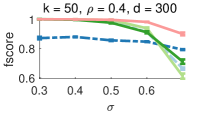
Synthetic data. We reproduce the procedure described in [8] for generating synthetic instances for the synchronisation of partial permutations. Four different parameters are considered for generating a problem instance: the universe size $d$, the number of objects $k$ that are to be matched, the observation rate $\rho$, and the error rate $\sigma$ (see [8] for details). One of these parameters varies in each experimental setting, while the others are kept fixed. Each individual experiment is repeated $5$ times with different random seeds. In Fig. 3 we compare the performance of MatchEig [31], MatchALS [51], Spectral [34], NmfSync [8] and Ours. The first row shows the fscore, and the second row the respective runtimes. Note that we did not run MatchALS on the larger instances since the runtime is prohibitively long. The methods MatchEig and MatchALS do not guarantee cycle consistency, and are thus shown as dashed lines. It can be seen that in most settings our method obtains superior performance in terms of the fscore, while being almost as fast as the most efficient methods that are also based on a spectral relaxation (MatchEig and Spectral).

The key contribution of this paper is an effective and efficient optimisation algorithm for addressing sparse optimisation problems over the Stiefel manifold. Given the fundamental nature of our contribution, we do not see any direct ethical concerns or negative societal impacts related to our work.

Overall, there are numerous opportunities to use the proposed method for various types of multi-matching problems over networks and graphs. The problem addressed is highly relevant within the fields of machine learning (e.g. for data canonicalisation to faciliate efficient learning with non-Euclidean data), computer vision (e.g. for 3D reconstruction in structure from motion, or image alignment), computer graphics (e.g. for bringing 3D shapes into correspondence) and other related areas.

The true power of permutation synchronisation methods appears when the number of objects to synchronise is large. With large quantities of data becoming increasingly available, the introduction of our scalable optimisation procedure that can account for orthogonality – while promoting sparsity and non-negativity – is an important contribution to the synchronisation community on the one hand. Moreover, on the other hand, it has the potential to have an impact on more general non-convex optimisation problems, particularly in the context of spectral relaxations of difficult and large combinatorial problems.

JT was supported by the Swedish Research Council (2019-04769).

References

- [1] CMU/VASC image database. http://www.cs.cmu.edu/afs/cs/project/vision/vasc/idb/www/html/motion/.
- [2] P.-A. Absil, C. G. Baker, and K. A. Gallivan. Trust-region methods on riemannian manifolds. Foundations of Computational Mathematics, 7(3):303–330, 2007.
- [3] P.-A. Absil, R. Mahony, and R. Sepulchre. Optimization algorithms on matrix manifolds. Princeton University Press, 2009.
- [4] P.-A. Absil, R. Mahony, R. Sepulchre, and P. Van Dooren. A grassmann–rayleigh quotient iteration for computing invariant subspaces. SIAM review, 44(1):57–73, 2002.
- [5] F. Arrigoni, B. Rossi, and A. Fusiello. Spectral synchronization of multiple views in se (3). SIAM Journal on Imaging Sciences, 9(4):1963–1990, 2016.
- [6] F. Bernard, C. Theobalt, and M. Moeller. DS*: Tighter Lifting-Free Convex Relaxations for Quadratic Matching Problems. In CVPR, 2018.
- [7] F. Bernard, J. Thunberg, P. Gemmar, F. Hertel, A. Husch, and J. Goncalves. A solution for multi-alignment by transformation synchronisation. In CVPR, 2015.
- [8] F. Bernard, J. Thunberg, J. Goncalves, and C. Theobalt. Synchronisation of partial multi-matchings via non-negative factorisations. Pattern Recognition, 92:146–155, 2019.
- [9] F. Bernard, J. Thunberg, P. Swoboda, and C. Theobalt. Hippi: Higher-order projected power iterations for scalable multi-matching. In CVPR, 2019.
- [10] F. Bernard, N. Vlassis, P. Gemmar, A. Husch, J. Thunberg, J. Goncalves, and F. Hertel. Fast correspondences for statistical shape models of brain structures. In Medical Imaging 2016: Image Processing, volume 9784, page 97840R. International Society for Optics and Photonics, 2016.
- [11] D. P. Bertsekas. Network Optimization: Continuous and Discrete Models. Athena Scientific, 1998.
- [12] T. Birdal, V. Golyanik, C. Theobalt, and L. J. Guibas. Quantum permutation synchronization. In CVPR, 2021.
- [13] T. Birdal and U. Simsekli. Probabilistic permutation synchronization using the riemannian structure of the birkhoff polytope. In CVPR, 2019.
- [14] N. Boumal, B. Mishra, P.-A. Absil, and R. Sepulchre. Manopt, a Matlab toolbox for optimization on manifolds. Journal of Machine Learning Research, 15(42):1455–1459, 2014.
- [15] A. Breloy, S. Kumar, Y. Sun, and D. P. Palomar. Majorization-minimization on the stiefel manifold with application to robust sparse pca. IEEE Transactions on Signal Processing, 69:1507–1520, 2021.
- [16] S. Chen, S. Ma, A. Man-Cho So, and T. Zhang. Proximal gradient method for nonsmooth optimization over the stiefel manifold. SIAM Journal on Optimization, 30(1):210–239, 2020.
- [17] T. Cour, P. Srinivasan, and J. Shi. Balanced graph matching. NIPS, 2006.
- [18] L. De Lathauwer, L. Hoegaerts, and J. Vandewalle. A grassmann-rayleigh quotient iteration for dimensionality reduction in ica. In International Conference on Independent Component Analysis and Signal Separation, pages 335–342. Springer, 2004.
- [19] A. Edelman, T. A. Arias, and S. T. Smith. The geometry of algorithms with orthogonality constraints. SIAM journal on Matrix Analysis and Applications, 20(2):303–353, 1998.
- [20] M. Gao, Z. Lähner, J. Thunberg, D. Cremers, and F. Bernard. Isometric multi-shape matching. In CVPR, 2021.
- [21] G. H. Golub and C. F. Van Loan. Matrix computations, volume 4. JHU press, 2013.
- [22] Q. Huang, Z. Liang, H. Wang, S. Zuo, and C. Bajaj. Tensor maps for synchronizing heterogeneous shape collections. ACM Transactions on Graphics (TOG), 38(4):1–18, 2019.
- [23] Q.-X. Huang and L. Guibas. Consistent shape maps via semidefinite programming. In Symposium on Geometry Processing, 2013.
- [24] R. Huang, J. Ren, P. Wonka, and M. Ovsjanikov. Consistent zoomout: Efficient spectral map synchronization. In Computer Graphics Forum, volume 39, pages 265–278. Wiley Online Library, 2020.
- [25] X. Huang, Z. Liang, X. Zhou, Y. Xie, L. J. Guibas, and Q. Huang. Learning transformation synchronization. In CVPR, 2019.
- [26] M. Leordeanu and M. Hebert. A Spectral Technique for Correspondence Problems Using Pairwise Constraints. In ICCV, 2005.
- [27] X. Li, S. Chen, Z. Deng, Q. Qu, Z. Zhu, and A. Man-Cho So. Weakly convex optimization over stiefel manifold using riemannian subgradient-type methods. SIAM Journal on Optimization, 31(3):1605–1634, 2021.
- [28] Y. Li and Y. Bresler. Global geometry of multichannel sparse blind deconvolution on the sphere. In NeurIPS, pages 1132–1143, 2018.
- [29] C. Lu, S. Yan, and Z. Lin. Convex sparse spectral clustering: Single-view to multi-view. IEEE Transactions on Image Processing, 25(6):2833–2843, 2016.
- [30] J. H. Manton. Optimization algorithms exploiting unitary constraints. IEEE Transactions on Signal Processing, 50(3):635–650, 2002.
- [31] E. Maset, F. Arrigoni, and A. Fusiello. Practical and Efficient Multi-View Matching. In ICCV, 2017.
- [32] J. Munkres. Algorithms for the Assignment and Transportation Problems. Journal of the Society for Industrial and Applied Mathematics, 5(1):32–38, Mar. 1957.
- [33] A. Ng, M. Jordan, and Y. Weiss. On spectral clustering: Analysis and an algorithm. NIPS, 14:849–856, 2001.
- [34] D. Pachauri, R. Kondor, and V. Singh. Solving the multi-way matching problem by permutation synchronization. In NIPS, 2013.
- [35] P. M. Pardalos, F. Rendl, and H. Wolkowicz. The Quadratic Assignment Problem - A Survey and Recent Developments. DIMACS Series in Discrete Mathematics, 1993.
- [36] Q. Qu, J. Sun, and J. Wright. Finding a sparse vector in a subspace: Linear sparsity using alternating directions. IEEE Transactions on Information Theory, 62(10):5855–5880, 2016.
- [37] Q. Qu, Y. Zhai, X. Li, Y. Zhang, and Z. Zhu. Geometric analysis of nonconvex optimization landscapes for overcomplete learning. In International Conference on Learning Representations, 2019.
- [38] Q. Qu, Z. Zhu, X. Li, M. C. Tsakiris, J. Wright, and R. Vidal. Finding the sparsest vectors in a subspace: Theory, algorithms, and applications. arXiv preprint arXiv:2001.06970, 2020.
- [39] Y. Shen, Q. Huang, N. Srebro, and S. Sanghavi. Normalized spectral map synchronization. NIPS, 29:4925–4933, 2016.
- [40] J. Song, P. Babu, and D. P. Palomar. Sparse generalized eigenvalue problem via smooth optimization. IEEE Transactions on Signal Processing, 63(7):1627–1642, 2015.
- [41] P. Swoboda, D. Kainmüller, A. Mokarian, C. Theobalt, and F. Bernard. A convex relaxation for multi-graph matching. In CVPR, 2019.
- [42] R. Tron, X. Zhou, C. Esteves, and K. Daniilidis. Fast multi-image matching via density-based clustering. In CVPR, 2017.
- [43] S. Umeyama. An eigendecomposition approach to weighted graph matching problems. IEEE transactions on pattern analysis and machine intelligence, 10(5):695–703, 1988.
- [44] U. Von Luxburg. A tutorial on spectral clustering. Statistics and computing, 17(4):395–416, 2007.
- [45] Q. Wang, J. Gao, and H. Li. Grassmannian manifold optimization assisted sparse spectral clustering. In Proceedings of the IEEE Conference on Computer Vision and Pattern Recognition, pages 5258–5266, 2017.
- [46] Z. Wen and W. Yin. A feasible method for optimization with orthogonality constraints. Mathematical Programming, 142(1):397–434, 2013.
- [47] Y. Xue, Y. Shen, V. Lau, J. Zhang, and K. B. Letaief. Blind data detection in massive mimo via -norm maximization over the stiefel manifold. IEEE Transactions on Wireless Communications, 2020.
- [48] J. Yan, X.-C. Yin, W. Lin, C. Deng, H. Zha, and X. Yang. A short survey of recent advances in graph matching. In Proceedings of the 2016 ACM on International Conference on Multimedia Retrieval, pages 167–174, 2016.
- [49] Y. Zhai, Z. Yang, Z. Liao, J. Wright, and Y. Ma. Complete dictionary learning via l4-norm maximization over the orthogonal group. Journal of Machine Learning Research, 21(165):1–68, 2020.
- [50] Y. Zhang, H.-W. Kuo, and J. Wright. Structured local optima in sparse blind deconvolution. IEEE Transactions on Information Theory, 66(1):419–452, 2019.
- [51] X. Zhou, M. Zhu, and K. Daniilidis. Multi-image matching via fast alternating minimization. In ICCV, 2015.
- [52] Z. Zhu, T. Ding, D. Robinson, M. Tsakiris, and R. Vidal. A linearly convergent method for non-smooth non-convex optimization on the grassmannian with applications to robust subspace and dictionary learning. NeurIPS, 32:9442–9452, 2019.
Appendix A Proofs
Proof of Lemma 1
Proof.
If the matrix is not symmetric, we can split into the sum of a symmetric part and skew-symmetric part . It holds that . Further, if is not positive semidefinite, we can shift its eigenvalues via to make it p.s.d. Since is constant for any scalar , the term does not affect the optimisers of Problem (1). Thus, we can replace in (1) by the p.s.d. matrix without affecting the optimisers. ∎
Proof of Lemma 2
Consider the eigenvalue decomposition of , i.e. , where contains the decreasingly ordered (nonnegative) eigenvalues on its diagonal and . For , this matrix can be written as the product of and another matrix , i.e., . So, instead of optimising over , we can optimise over . Let the -th row of be denoted as for . It holds that . Thus, an equivalent formulation of Problem (1) is the optimisation problem