Sparse random graphs: Eigenvalues and Eigenvectors

In this paper, we consider two models of random graphs, the Erdős-Rényi random graph $G(n,p)$ and the random regular graph $G_{n,d}$. Given a real number $p=p(n)$,$0\leq p\leq 1$, the Erdős-Rényi graph on a vertex set of size $n$ is obtained by drawing an edge between each pair of vertices, randomly and independently, with probability $p$. On the other hand, $G_{n,d}$, where $d=d(n)$ denotes the degree, is a random graph chosen uniformly from the set of all simple $d$-regular graphs on $n$ vertices. These are basic models in the theory of random graphs. For further information, we refer the readers to the excellent monographs $\cite[cite]{[\@@bibref{}{bollobas}{}{}]},\cite[cite]{[\@@bibref{}{janson}{}{}]}$ and survey [33].

Given a graph $G$ on $n$ vertices, the adjacency matrix $A$ of $G$ is an $n\times n$ matrix whose entry $a_{ij}$ equals one if there is an edge between the vertices $i$ and $j$ and zero otherwise. All diagonal entries $a_{ii}$ are defined to be zero. The eigenvalues and eigenvectors of $A$ carry valuable information about the structure of the graph and have been studied by many researchers for quite some time, with both theoretical and practical motivations (see, for example, $\cite[cite]{[\@@bibref{}{bauer}{}{}]},\cite[cite]{[\@@bibref{}{bhamidi}{}{}]},\cite[cite]{[\@@bibref{}{feige}{}{}]},\cite[cite]{[\@@bibref{}{semerjian}{}{}]}$ $\cite[cite]{[\@@bibref{}{FK1981}{}{}]},\cite[cite]{[\@@bibref{}{fried1991}{}{}]},\cite[cite]{[\@@bibref{}{fried2003}{}{}]}$, $\cite[cite]{[\@@bibref{}{fried1993}{}{}]},\cite[cite]{[\@@bibref{}{tvrandom}{}{}]},\cite[cite]{[\@@bibref{}{erdos2009semi}{}{}]}$, $\cite[cite]{[\@@bibref{}{shi2000}{}{}]},\cite[cite]{[\@@bibref{}{pothen1990}{}{}]}$).

The goal of this paper is to study the eigenvalues and eigenvectors of $G(n,p)$ and $G_{n,d}$. We are going to consider:

• •

  The global law for the limit of the empirical spectral distribution (ESD) of adjacency matrices of $G(n,p)$ and $G_{n,d}$. For $p=\omega(1/n)$, it is well-known that eigenvalues of $G(n,p)$ (after a proper scaling) follows Wigner’s semicircle law (we include a short proof in the Appendix A for completeness). Our main new result shows that the same law holds for random regular graph with $d\rightarrow\infty$ with $n$. This complements the well known result of McKay for the case when $d$ is an absolute constant (McKay’s law) and extends recent results of Dumitriu and Pal [9] (see Section 1.2 for more discussion).

• •

  Bound on the infinity norm of the eigenvectors. We first prove that the infinity norm of any (unit) eigenvector $v$ of $G(n,p)$ is almost surely $o(1)$ for $p=\omega(\log n/n)$. This gives a positive answer to a question raised by Dekel, Lee and Linial [7]. Furthermore, we can show that $v$ satisfies the bound $\|v\|_{\infty}=O\left(\sqrt{\log^{2.2}g(n){\log n}/{np}}\right)$ for $p=\omega(\log n/n)=g(n)\log n/n$, as long as the corresponding eigenvalue is bounded away from the (normalized) extremal values $-2$ and $2$.

We finish this section with some notation and conventions.

Given an $n\times n$ symmetric matrix $M$, we denote its $n$ eigenvalues as

$${\lambda}_{1}{(M)}\leq{\lambda}_{2}{(M)}\leq\ldots\leq{\lambda}_{n}{(M)},$$

and let $u_{1}(M),\ldots,u_{n}(M)\in\mathbb{R}^{n}$ be an orthonormal basis of eigenvectors of $M$ with

$$Mu_{i}(M)={\lambda}_{i}u_{i}(M).$$

The empirical spectral distribution (ESD) of the matrix $M$ is a one-dimensional function

$$F^{\bf M}_{n}(x)=\frac{1}{n}|\{1\leq j\leq n:\lambda_{j}(M)\leq x\}|,$$

where we use $|\mathbf{I}|$ to denote the cardinality of a set $\mathbf{I}$.

Let $A_{n}$ be the adjacency matrix of $G(n,p)$. Thus $A_{n}$ is a random symmetric $n\times n$ matrix whose upper triangular entries are iid copies of a real random variable $\xi$ and diagonal entries are $0$. $\xi$ is a Bernoulli random variable that takes values $1$ with probability $p$ and $0$ with probability $1-p$.

$$\mathbb{E}\xi=p,\mathbb{V}ar{\xi}=p(1-p)={\sigma}^{2}.$$

Usually it is more convenient to study the normalized matrix

$$M_{n}=\frac{1}{\sigma}(A_{n}-pJ_{n})$$

where $J_{n}$ is the $n\times n$ matrix all of whose entries are 1. $M_{n}$ has entries with mean zero and variance one. The global properties of the eigenvalues of $A_{n}$ and $M_{n}$ are essentially the same (after proper scaling), thanks to the following lemma

The main advantage of this definition is that if we have a polynomial number of events, each of which holds with overwhelming probability, then their intersection also holds with overwhelming probability.

Asymptotic notation is used under the assumption that $n\rightarrow\infty$. For functions $f$ and $g$ of parameter $n$, we use the following notation as $n\rightarrow\infty$: $f=O(g)$ if $|f|/|g|$ is bounded from above; $f=o(g)$ if $f/g\rightarrow 0$; $f=\omega(g)$ if $|f|/|g|\rightarrow\infty$, or equivalently, $g=o(f)$; $f=\Omega(g)$ if $g=O(f)$; $f=\Theta(g)$ if $f=O(g)$ and $g=O(f)$.

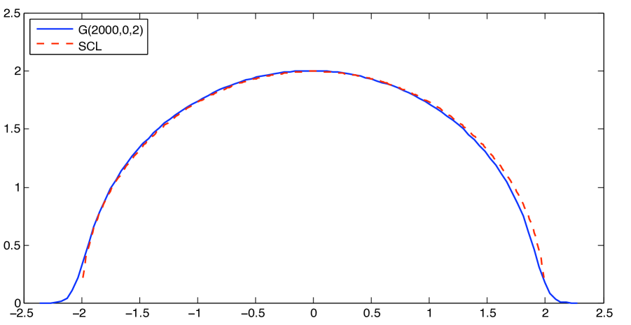
In 1950s, Wigner [32] discovered the famous semi-circle for the limiting distribution of the eigenvalues of random matrices. His proof extends, without difficulty, to the adjacency matrix of $G(n,p)$, given that $np\rightarrow\infty$ with $n$. (See Figure 1 for a numerical simulation)

If $np=O(1)$, the semicircle law no longer holds. In this case, the graph almost surely has $\Theta(n)$ isolated vertices, so in the limiting distribution, the point $0$ will have positive constant mass.

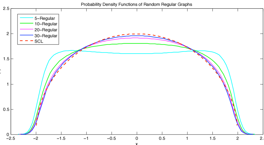
The case of random regular graph, $G_{n,d}$, was considered by McKay [21] about 30 years ago. He proved that if $d$ is fixed, and $n\rightarrow\infty$, then the limiting density function is

$$\displaystyle f_{d}(x)=\left\{\begin{array}[]{ll}\frac{d\sqrt{4(d-1)-x^{2}}}{2\pi(d^{2}-x^{2})},&\mbox{if $|x|\leq 2\sqrt{d-1}$};\\ \\ 0&\mbox{otherwise}.\end{array}\right.$$

This is usually referred to as McKay or Kesten-McKay law.

It is easy to verify that as $d\rightarrow\infty$, if we normalize the variable $x$ by $\sqrt{d-1}$, then the above density converges to the semicircle distribution on $[-2,2]$. In fact, a numerical simulation shows the convergence is quite fast(see Figure 2).

It is thus natural to conjecture that Theorem 1.3 holds for $G_{n,d}$ with $d\rightarrow\infty$. Let $A^{\prime}_{n}$ be the adjacency matrix of $G_{n,d}$, and set

$$M^{\prime}_{n}=\frac{1}{\sqrt{\frac{d}{n}(1-\frac{d}{n})}}(A^{\prime}_{n}-\frac{d}{n}J).$$

Nothing has been proved about this conjecture, until recently. In [9], Dimitriu and Pal showed that the conjecture holds for $d$ tending to infinity slowly, $d=n^{o(1)}$. Their method does not extend to larger $d$.

We are going to establish Conjecture 1.4 in full generality. Our method is very different from that of [9].

Without loss of generality we may assume $d\leq n/2$, since the adjacency matrix of the complement graph of $G_{n,d}$ may be written as $J_{n}-A^{\prime}_{n}$, thus by Lemma 1.1 will have the spectrum interlacing between the set $\{-\lambda_{n}(A^{\prime}_{n}),\dots,-\lambda_{1}(A^{\prime}_{n})\}$. Since the semi-circular distribution is symmetric, the ESD of $G_{n,d}$ will converges to semi-circular law if and only if the ESD of its complement does.

Theorem 1.5 is a direct consequence of the following stronger result, which shows convergence at small scales. For an interval $I$ let $N^{\prime}_{I}$ be the number of eigenvalues of $M^{\prime}_{n}$ in $I$.

Relatively little is known for eigenvectors in both random graph models under study. In [7], Dekel, Lee and Linial, motivated by the study of nodal domains, raised the following question.

Later, in their journal paper [8], the authors added one sharper question.

The bound $n^{-1/2+o(1)}$ was also conjectured by the second author of this paper in an NSF proposal (submitted Oct 2008). He and Tao [30] proved this bound for eigenvectors corresponding to the eigenvalues in the bulk of the spectrum for the case $p=1/2$. If one defines the adjacency matrix by writting $-1$ for non-edges, then this bound holds for all eigenvectors [30, 29].

The above two questions were raised under the assumption that $p$ is a constant in the interval $(0,1)$. For $p$ depending on $n$, the statements may fail. If $p\leq\frac{(1-\epsilon)\log n}{n}$, then the graph has (with high probability) isolated vertices and so one cannot expect that $\|u\|_{\infty}=o(1)$ for every eigenvector $u$. We raise the following questions:

Similarly, we can ask the above questions for $G_{n,d}$:

As far as random regular graphs is concerned, Dumitriu and Pal [9] and Brook and Lindenstrauss [5] showed that for any normalized eigenvector of a sparse random regular graph is delocalized in the sense that one can not have too much mass on a small set of coordinates. The readers may want to consult their papers for explicit statements.

We generalize our questions by the following conjectures:

In this paper, we focus on $G(n,p)$. Our main result settles (positively) Question 1.8 and almost Question 1.10 . This result follows from Corollary 2.3 obtained in Section 2.

For Questions 1.9 and 1.11, we obtain a good quantitative bound for those eigenvectors which correspond to eigenvalues bounded away from the edge of the spectrum.

For convenience, in the case when $p=\omega(\log n/n)\in(0,1)$, we write

$$p=\frac{g(n)\log n}{n},$$

where $g(n)$ is a positive function such that $g(n)\rightarrow\infty$ as $n\rightarrow\infty$ ($g(n)$ can tend to $\infty$ arbitrarily slowly).

The proofs are adaptations of a recent approach developed in random matrix theory (as in [30],[29],[10], [11]). The main technical lemma is a concentration theorem about the number of eigenvalues on a finer scale for $p=\omega(\log n/n)$.

We use the method of comparison. An important lemma is the following

For the range $p\geq\log^{2}n/n$, Lemma 2.1 is a consequence of a result of Shamir and Upfal [26] (see also [20]). For smaller values of $np$, McKay and Wormald [23] calculated precisely the probability that $G(n,p)$ is $np$-regular, using the fact that the joint distribution of the degree sequence of $G(n,p)$ can be approximated by a simple model derived from independent random variables with binomial distribution. Alternatively, one may calculate the same probability directly using the asymptotic formula for the number of $d$-regular graphs on $n$ vertices (again by McKay and Wormald [22]). Either way, for $p=o(1/\sqrt{n})$, we know that

$${\hbox{\bf P}}(G(n,p)\text{ is }np\text{-regular})\geq\Theta(\exp(-n\log(\sqrt{np})).$$

which is better than claimed in Lemma 2.1.

Another key ingredient is the following concentration lemma, which may be of independent interest.

Apply Lemma 2.2 for the normalized adjacency matrix $M_{n}$ of $G(n,p)$ with $K=1/\sqrt{p}$ we obtain

By Corollary 2.3 and Lemma 2.1, the probability that $N_{I}$ fails to be close to the expected value in the model $G(n,p)$ is much smaller than the probability that $G(n,p)$ is $np$-regular. Thus the probability that $N_{I}$ fails to be close to the expected value in the model $G_{n,d}$ where $d=np$ is the ratio of the two former probabilities, which is $O(\exp(-cn\sqrt{np}\log np))$ for some small positive constant $c$. Thus, Theorem 1.6 is proved, depending on Lemma 2.2 which we turn to next.

Assume $I=[a,b]$ and $a-(-2)<2-b$.

We will use the approach of Guionnet and Zeitouni in [18]. Consider a random Hermitian matrix $W_{n}$ with independent entries $w_{ij}$ with support in a compact region $S$. Let $f$ be a real convex $L$-Lipschitz function and define

$$Z:=\sum_{i=1}^{n}f(\lambda_{i})$$

where $\lambda_{i}$’s are the eigenvalues of $\frac{1}{\sqrt{n}}W_{n}$. We are going to view $Z$ as the function of the atom variables $w_{ij}$. For our application we need $w_{ij}$ to be random variables with mean zero and variance 1, whose absolute values are bounded by a common constant $K$.

The following concentration inequality is from [18]

In order to apply Lemma 2.5 for $N_{I}$ and $M$, it is natural to consider

$$Z:=N_{I}=\sum_{i=1}^{n}\chi_{I}(\lambda_{i})$$

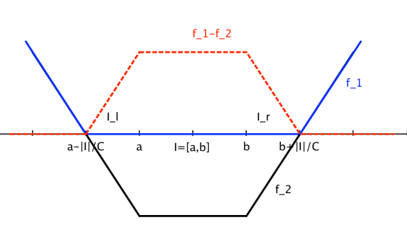
where $\chi_{I}$ is the indicator function of $I$ and $\lambda_{i}$ are the eigenvalues of $\frac{1}{\sqrt{n}}M_{n}$. However, this function is neither convex nor Lipschitz. As suggested in [18], one can overcome this problem by a proper approximation. Define $I_{l}=[a-\frac{|I|}{C},a]$, $I_{r}=[b,b+\frac{|I|}{C}]$ and construct two real functions $f_{1},f_{2}$ as follows(see Figure 3):

$$f_{1}(x)=\Bigg{\{}\begin{array}[]{ll}-\frac{C}{|I|}(x-a)-1&\text{if }x\in(-\infty,a-\frac{|I|}{C})\\ 0&\text{if }x\in I\cup I_{l}\cup I_{r}\\ \frac{C}{|I|}(x-b)-1&\text{if }x\in(b+\frac{|I|}{C},\infty)\end{array}$$

$$f_{2}(x)=\Bigg{\{}\begin{array}[]{ll}-\frac{C}{|I|}(x-a)-1&\text{if }x\in(-\infty,a)\\ -1&\text{if }x\in I\\ \frac{C}{|I|}(x-b)-1&\text{if }x\in(b,\infty)\end{array}$$

where $C$ is a constant to be chosen later. Note that $f_{j}$’s are convex and $\frac{C}{|I|}$-Lipschitz. Define

$$X_{1}=\sum_{i=1}^{n}f_{1}(\lambda_{i}),\ X_{2}=\sum_{i=1}^{n}f_{2}(\lambda_{i})$$

and apply Lemma 2.5 with $T=\frac{\delta}{8}n\int_{I}\rho_{sc}(t)dt$ for $X_{1}$ and $X_{2}$. Thus, we have

$\displaystyle{\hbox{\bf P}}(|X_{j}-{\hbox{\bf E}}(X_{j})|\geq\frac{\delta}{8}n\int_{I}\rho_{sc}(t)dt)$

$\displaystyle\leq 4\exp(-c\frac{\delta^{2}n^{2}|I|^{2}(\int_{I}\rho_{sc}(t)dt)^{2}}{K^{2}C^{2}}).$

At this point we need to estimate the value of $\int_{I}\rho_{sc}(t)dt$. There are two cases: if $I$ is in the “bulk” i.e. $I\subset[-2+\epsilon,2-\epsilon]$ for some positive absolute constant $\epsilon$, then $\int_{I}\rho_{sc}(t)dt=\alpha|I|$ where $\alpha$ is a constant depending on $\epsilon$. But if $I$ is very near the edge of $[-2,2]$ i.e. $a-(-2)<|I|=o(1)$, then $\int_{I}\rho_{sc}(t)dt=\alpha^{\prime}|I|^{3/2}$ for some absolute constant $\alpha^{\prime}$. Thus in both case we have

$${\hbox{\bf P}}(|X_{j}-{\hbox{\bf E}}(X_{j})|\geq\frac{\delta}{8}n\int_{I}\rho_{sc}(t)dt)\leq 4\exp(-c_{1}\frac{\delta^{2}n^{2}|I|^{5}}{K^{2}C^{2}})$$

Let $X=X_{1}-X_{2}$, then

$${\hbox{\bf P}}(|X-{\hbox{\bf E}}(X)|\geq\frac{\delta}{4}n\int_{I}\rho_{sc}(t)dt)\leq O(\exp(-c_{1}\frac{\delta^{2}n^{2}|I|^{5}}{K^{2}C^{2}})).$$

Now we compare $X$ to $Z$, making use of a result of Götze and Tikhomirov [17]. We have ${\hbox{\bf E}}(X-Z)\leq{\hbox{\bf E}}(N_{I_{l}}+N_{I_{r}})$. In [17], Götze and Tikhomirov obtained a convergence rate for ESD of Hermitian random matrices whose entries have mean zero and variance one, which implies that for any $I\subset[-2,2]$

$$|{\hbox{\bf E}}(N_{I})-n\int_{I}\rho_{sc}(t)dt|<\beta n\sqrt{\frac{M_{4}}{n}},$$

where $\beta$ is an absolute constant, $M_{4}=\sup_{i,j}{\hbox{\bf E}}(|\omega_{ij}|^{4})$. Thus

$${\hbox{\bf E}}(X)\leq{\hbox{\bf E}}(Z)+n\int_{I_{l}\cup I_{r}}\rho_{sc}(t)dt+\beta n\sqrt{\frac{M_{4}}{n}}.$$

In the “edge” case we can choose $C=(4/\delta)^{2/3}$, then because $|I|\geq\Omega(\delta^{-2/3}(M_{4}/n)^{1/3})$, we have

$$n\int_{I_{l}\cup I_{r}}\rho_{sc}(t)dt=\Theta(n(\frac{|I|}{C})^{3/2})>\Omega(n\sqrt{\frac{M_{4}}{n}})$$

and

$$n\int_{I_{l}\cup I_{r}}\rho_{sc}(t)dt+\beta n\sqrt{\frac{M_{4}}{n}}=\Theta(n(\frac{|I|}{C})^{3/2})=\Theta(\frac{\delta}{4}n\int_{I}\rho_{sc}(t)dt).$$

In the “bulk” case we choose $C=4/\delta$, then

$$n\int_{I_{l}\cup I_{r}}\rho_{sc}(t)dt+\beta n\sqrt{\frac{M_{4}}{n}}=\Theta(n\frac{|I|}{C})=\Theta(\frac{\delta}{4}n\int_{I}\rho_{sc}(t)dt).$$

Therefore in both cases, with probability at least $1-O(\exp(-c_{1}\frac{\delta^{4}n^{2}|I|^{5}}{K^{2}}))$, we have

$$Z\leq X\leq{\hbox{\bf E}}(X)+\frac{\delta}{4}n\int_{I}\rho_{sc}(t)dt<{\hbox{\bf E}}(Z)+\frac{\delta}{2}n\int_{I}\rho_{sc}(t)dt.$$

The convergence rate result of Götze and Tikhomirov again gives

$${\hbox{\bf E}}(N_{I})<n\int_{I}\rho_{sc}(t)dt+\beta n\sqrt{\frac{M_{4}}{n}}<(1+\frac{\delta}{2})n\int_{I}\rho_{sc}(t)dt,$$

hence with probability at least $1-O(\exp(-c_{1}\frac{\delta^{4}n^{2}|I|^{5}}{K^{2}}))$

$$Z<(1+\delta)n\int_{I}\rho_{sc}(t)dt,$$

which is the desires upper bound.

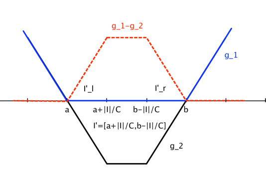
The lower bound is proved using a similar argument. Let $I^{\prime}=[a+\frac{|I|}{C},b-\frac{|I|}{C}]$, $I^{\prime}_{l}=[a,a+\frac{|I|}{C}]$, $I^{\prime}_{r}=[b-\frac{|I|}{C},b]$ where $C$ is to be chosen later and define two functions $g_{1}$, $g_{2}$ as follows (see Figure 3):

$$g_{1}(x)=\Bigg{\{}\begin{array}[]{ll}-\frac{C}{|I|}(x-a)&\text{if }x\in(-\infty,a)\\ 0&\text{if }x\in I^{\prime}\cup I^{\prime}_{l}\cup I^{\prime}_{r}\\ \frac{C}{|I|}(x-b)&\text{if }x\in(b,\infty)\end{array}$$

$$g_{2}(x)=\Bigg{\{}\begin{array}[]{ll}-\frac{C}{|I|}(x-a)&\text{if }x\in(-\infty,a+\frac{|I|}{C})\\ -1&\text{if }x\in I^{\prime}\\ \frac{C}{|I|}(x-b)&\text{if }x\in(b-\frac{|I|}{C},\infty)\end{array}$$

Define

$$Y_{1}=\sum_{i=1}g_{1}(\lambda_{i}),\ Y_{2}=\sum_{i=1}g_{2}(\lambda_{i}).$$

Applying Lemma 2.5 with $T=\frac{\delta}{8}n\int_{I}\rho_{sc}(t)dt$ for $Y_{j}$ and using the estimation for $\int_{I}\rho(t)dt$ as above, we have

$${\hbox{\bf P}}(|Y_{j}-{\hbox{\bf E}}(Y_{j})|\geq\frac{\delta}{8}n\int_{I}\rho_{sc}(t)dt)\leq 4\exp(-c_{2}\frac{\delta^{2}n^{2}|I|^{5}}{K^{2}C^{2}}).$$

Let $Y=Y_{1}-Y_{2}$, then

$${\hbox{\bf P}}(|Y-{\hbox{\bf E}}(Y)|\geq\frac{\delta}{4}n\int_{I}\rho_{sc}(t)dt)\leq O(\exp(-c_{2}\frac{\delta^{2}n^{2}|I|^{5}}{K^{2}C^{2}})).$$

We have ${\hbox{\bf E}}(Z-Y)\leq{\hbox{\bf E}}(N_{I^{\prime}_{l}}+N_{I^{\prime}_{r}})$. A similar argument as in the proof of the upper bound (using the convergence rate of Götze and Tikhomirov) shows

$${\hbox{\bf E}}(Y)\geq{\hbox{\bf E}}(Z)-n\int_{I^{\prime}_{l}\cup I^{\prime}_{r}}\rho_{sc}(t)dt-\beta n\sqrt{\frac{M_{4}}{n}}>E(Z)-\frac{\delta}{4}n\int_{I}\rho_{sc}(t)dt.$$

Therefore with probability at least $1-O(\exp(-c_{2}\frac{\delta^{2}n^{2}|I|^{5}}{K^{2}C^{2}}))$, we have

$$Z\geq Y\geq{\hbox{\bf E}}(Y)-\frac{\delta}{4}n\int_{I}\rho_{sc}(t)dt>{\hbox{\bf E}}(Z)-\frac{\delta}{2}n\int_{I}\rho_{sc}(t)dt,$$

and by the convergence rate, with probability at least $1-O(\exp(-c2\frac{\delta^{2}n^{2}|I|^{5}}{K^{2}C^{2}}))$

$$Z>(1-\delta)n\int_{I}\rho_{sc}(t)dt.$$

Thus, Theorem 2.2 is proved.

$A_{n}$ is the adjacency matrix of $G(n,p)$. In the proofs of Theorem 1.16 and Theorem 1.17, we actually work with the eigenvectors of a perturbed matrix

$$A_{n}+\epsilon N_{n},$$

where $\epsilon=\epsilon(n)>0$ can be arbitrarily small and $N_{n}$ is a symmetric random matrix whose upper triangular elements are independent with a standard Gaussian distribution.

The entries of $A_{n}+\epsilon N_{n}$ are continuous and thus with probability 1, the eigenvalues of $A_{n}+\epsilon N_{n}$ are simple. Let

$$\mu_{1}<\ldots<\mu_{n}$$

be the ordered eigenvalues of $A_{n}+\epsilon N_{n}$, which have a unique orthonormal system of eigenvectors $\{w_{1},\ldots,w_{n}\}$. By the Cauchy interlacing principle, the eigenvalues of $A_{n}+\epsilon N_{n}$ are different from those of its principle minors, which satisfies a condition of Lemma 3.2.

Let $\lambda_{i}$’s be the eigenvalue of $A_{n}$ with multiplicity $k_{i}$ defined as follows:

$$\ldots\lambda_{i-1}<\lambda_{i}=\lambda_{i+1}=\ldots=\lambda_{i+k_{i}}<\lambda_{i+k_{i}+1}\ldots$$

By Weyl’s theorem, one has for every $1\leq j\leq n$,

$$|\lambda_{j}-\mu_{j}|\leq\epsilon||N_{n}||_{\text{op}}=O(\epsilon\sqrt{n})$$

(3.1)

Thus the behaviors of eigenvalues of $A_{n}$ and $A_{n}+\epsilon N_{n}$ are essentially the same by choosing $\epsilon$ sufficiently small. And everything (except Lemma 3.2) we used in the proofs of Theorem 1.16 and Theorem 1.17 for $A_{n}$ also applies for $A_{n}+\epsilon N_{n}$ by a continuity argument. We will not distinguish $A_{n}$ from $A_{n}+\epsilon N_{n}$ in the proofs.

The following lemma will allow us to transfer the eigenvector delocaliztion results of $A_{n}+\epsilon N_{n}$ to those of $A_{n}$ at some expense.

References

- [1] Z.D. Bai. Methodologies in spectral analysis of large dimensional random matrices, a review. In Advances in statistics: proceedings of the conference in honor of Professor Zhidong Bai on his 65th birthday, National University of Singapore, 20 July 2008, volume 9, page 174. World Scientific Pub Co Inc, 2008.
- [2] M. Bauer and O. Golinelli. Random incidence matrices: moments of the spectral density. Journal of Statistical Physics, 103(1):301–337, 2001.
- [3] S. Bhamidi, S.N. Evans, and A. Sen. Spectra of large random trees. Arxiv preprint arXiv:0903.3589, 2009.
- [4] B. Bollobás. Random graphs. Cambridge Univ Pr, 2001.
- [5] S. Brooks and E. Lindenstrauss. Non-localization of eigenfunctions on large regular graphs. Arxiv preprint arXiv:0912.3239, 2009.
- [6] F. Chung, L. Lu, and V. Vu. The spectra of random graphs with given expected degrees. Internet Mathematics, 1(3):257–275, 2004.
- [7] Y. Dekel, J. Lee, and N. Linial. Eigenvectors of random graphs: Nodal domains. In APPROX ’07/RANDOM ’07: Proceedings of the 10th International Workshop on Approximation and the 11th International Workshop on Randomization, and Combinatorial Optimization. Algorithms and Techniques, pages 436–448, Berlin, Heidelberg, 2007. Springer-Verlag.
- [8] Y. Dekel, J. Lee, and N. Linial. Eigenvectors of random graphs: Nodal domains. Approximation, Randomization, and Combinatorial Optimization. Algorithms and Techniques, pages 436–448, 2008.
- [9] I. Dumitriu and S. Pal. Sparse regular random graphs: spectral density and eigenvectors. Arxiv preprint arXiv:0910.5306, 2009.
- [10] L. Erdos, B. Schlein, and H.T. Yau. Semicircle law on short scales and delocalization of eigenvectors for Wigner random matrices. Ann. Probab, 37(3):815–852, 2009.
- [11] L. Erdos, B. Schlein, and H.T. Yau. Local semicircle law and complete delocalization for Wigner random matrices. Accepted in Comm. Math. Phys. Communications in Mathematical Physics, 287(2):641–655, 2010.
- [12] U. Feige and E. Ofek. Spectral techniques applied to sparse random graphs. Random Structures and Algorithms, 27(2):251, 2005.
- [13] J. Friedman. On the second eigenvalue and random walks in random -regular graphs. Combinatorica, 11(4):331–362, 1991.
- [14] J. Friedman. Some geometric aspects of graphs and their eigenfunctions. Duke Math. J, 69(3):487–525, 1993.
- [15] J. Friedman. A proof of Alon’s second eigenvalue conjecture. In Proceedings of the thirty-fifth annual ACM symposium on Theory of computing, pages 720–724. ACM, 2003.
- [16] Z Füredi and J. Komlós. The eigenvalues of random symmetric matrices. Combinatorica, 1(3):233–241, 1981.
- [17] F. Götze and A. Tikhomirov. Rate of convergence to the semi-circular law. Probability Theory and Related Fields, 127(2):228–276, 2003.
- [18] A. Guionnet and O. Zeitouni. Concentration of the spectral measure for large matrices. Electron. Comm. Probab, 5:119–136, 2000.
- [19] S. Janson, T. Łuczak, and A. Ruciński. Random graphs. Citeseer, 2000.
- [20] M. Krivelevich, B. Sudakov, V.H. Vu, and N.C. Wormald. Random regular graphs of high degree. Random Structures and Algorithms, 18(4):346–363, 2001.
- [21] B.D. McKay. The expected eigenvalue distribution of a large regular graph. Linear Algebra and its Applications, 40:203–216, 1981.
- [22] B.D. McKay and N.C. Wormald. Asymptotic enumeration by degree sequence of graphs with degrees . Combinatorica 11 , no. 4, 369–382., 1991.
- [23] B.D. McKay and N.C. Wormald. The degree sequence of a random graph. I. The models. Random Structures Algorithms 11, no. 2, 97–117, 1997.
- [24] A. Pothen, H.D. Simon, and K.P. Liou. Partitioning sparse matrices with eigenvectors of graphs. SIAM Journal on Matrix Analysis and Applications, 11:430, 1990.
- [25] G. Semerjian and L.F. Cugliandolo. Sparse random matrices: the eigenvalue spectrum revisited. Journal of Physics A: Mathematical and General, 35:4837–4851, 2002.
- [26] E Shamir and E Upfal. Large regular factors in random graphs. Convexity and graph theory (Jerusalem, 1981), 1981.
- [27] J. Shi and J. Malik. Normalized cuts and image segmentation. IEEE Transactions on pattern analysis and machine intelligence, 22(8):888–905, 2000.
- [28] G.W. Stewart and Ji-guang. Sun. Matrix perturbation theory. Academic press New York, 1990.
- [29] T. Tao and V. Vu. Random matrices: Universality of local eigenvalue statistics up to the edge. Communications in Mathematical Physics, pages 1–24, 2010.
- [30] T. Tao and V. Vu. Random matrices: Universality of the local eigenvalue statistics, submitted. Institute of Mathematics, University of Munich, Theresienstr, 39, 2010.
- [31] V. Vu. Random discrete matrices. Horizons of Combinatorics, pages 257–280, 2008.
- [32] E.P. Wigner. On the distribution of the roots of certain symmetric matrices. Annals of Mathematics, 67(2):325–327, 1958.
- [33] N.C. Wormald. Models of random regular graphs. London Mathematical Society Lecture Note Series, pages 239–298, 1999.