Sparse recovery by non-convex optimization – instance optimality
Abstract
In this note, we address the theoretical properties of , a class of compressed sensing decoders that rely on minimization with to recover estimates of sparse and compressible signals from incomplete and inaccurate measurements. In particular, we extend the results of Candès, Romberg and Tao [4] and Wojtaszczyk [30] regarding the decoder , based on minimization, to with . Our results are two-fold. First, we show that under certain sufficient conditions that are weaker than the analogous sufficient conditions for the decoders are robust to noise and stable in the sense that they are instance optimal for a large class of encoders. Second, we extend the results of Wojtaszczyk to show that, like , the decoders are instance optimal in probability provided the measurement matrix is drawn from an appropriate distribution.
1 Introduction
The sparse recovery problem received a lot of attention lately, both because of its role in transform coding with redundant dictionaries (e.g., [28, 29, 9]), and perhaps more importantly because it inspired compressed sensing [13, 3, 4], a novel method of acquiring signals with certain properties more efficiently compared to the classical approach based on Nyquist-Shannon sampling theory. Define to be the set of all -sparse vectors, i.e.,
and define compressible vectors as vectors that can be well approximated in . Let denote the best -term approximation error of in (quasi-)norm where , i.e.,
Throughout the text, denotes an real matrix where . Let the associated encoder be the map (also denoted by ). The transform coding and compressed sensing problems mentioned above require the existence of decoders, say , with roughly the following properties:
-
(C1)
whenever with sufficiently small .
-
(C2)
, where the norms are appropriately chosen. Here denotes measurement error, e.g., thermal and computational noise.
-
(C3)
can be computed efficiently (in some sense).
Below, we denote the (in general noisy) encoding of by , i.e.,
| (1) |
In general, the problem of constructing decoders with properties (C1)-(C3) is non-trivial (even in the noise-free case) as is overcomplete, i.e., the linear system of equations in (1) is underdetermined, and thus, if consistent, it admits infinitely many solutions. In order for a decoder to satisfy (C1)-(C3), it must choose the “correct solution” among these infinitely many solutions. Under the assumption that the original signal is sparse, one can phrase the problem of finding the desired solution as an optimization problem where the objective is to maximize an appropriate “measure of sparsity” while simultaneously satisfying the constraints defined by (1). In the noise-free case, i.e., when in (1), under certain conditions on the matrix , i.e., if is in general position, there is a decoder which satisfies for all whenever , e.g., see [14]. This can be explicitly computed via the optimization problem
| (2) |
Here denotes the number of non-zero entries of the vector , equivalently its so-called -norm. Clearly, the sparsity of is reflected by its -norm.
1.1 Decoding by minimization
As mentioned above, exactly if is sufficiently sparse depending on the matrix . However, the associated optimization problem is combinatorial in nature, thus its complexity grows quickly as becomes much larger than . Naturally, one then seeks to modify the optimization problem so that it lends itself to solution methods that are more tractable than combinatorial search. In fact, in the noise-free setting, the decoder defined by minimization, given by
| (3) |
recovers exactly if is sufficiently sparse and the matrix has certain properties (e.g., [6, 4, 14, 15, 9, 26]). In particular, it has been shown in [4] that if and satisfies a certain restricted isometry property, e.g., or more generally for some such that , then (in what follows, denotes the set of positive integers, i.e., ). Here are the -restricted isometry constants of , as introduced by Candès, Romberg and Tao (see, e.g., [4]), defined as the smallest constants satisfying
| (4) |
for every . Throughout the paper, using the notation of [30], we say that a matrix satisfies if .
Checking whether a given matrix satisfies a certain RIP is computationally intensive, and becomes rapidly intractable as the size of the matrix increases. On the other hand, there are certain classes of random matrices which have favorable RIP. In fact, let be an matrix the columns of which are independent, identically distributed (i.i.d.) random vectors with any sub-Gaussian distribution. It has been shown that satisfies with any when
| (5) |
with probability greater than (see, e.g., [1],[5],[6]), where and are positive constants that only depend on and on the actual distribution from which is drawn.
In addition to recovering sparse vectors from error-free observations, it is important that the decoder be robust to noise and stable with regards to the “compressibility” of . In other words, we require that the reconstruction error scale well with the measurement error and with the “non-sparsity” of the signal (i.e., (C2) above). For matrices that satisfy , with for some such that , it has been shown in [4] that there exists a feasible decoder for which the approximation error scales linearly with the measurement error and with . More specifically, define the decoder
| (6) |
The following theorem of Candès et al. in [4] provides error guarantees when is not sparse and when the observation is noisy.
Theorem 1
[4] Fix , suppose that is arbitrary, and let where . If satisfies , then
| (7) |
For reasonable values of , the constants are well behaved; e.g., and for .
Remark 2
This means that given , and is sufficiently sparse, recovers the underlying sparse signal within the noise level. Consequently the recovery is perfect if .
Remark 3
By explicitly assuming to be sparse, Candès et. al. [4] proved a version of the above result with smaller constants, i.e., for with and ,
| (8) |
where .
Remark 4
In the noise free case, i.e., when , the reconstruction error in Theorem 1 is bounded above by , see (7). This upper bound would sharpen if one could replace with on the right hand side of (7) (note that can be large even if all the entries of the reconstruction error are small but nonzero; this follows from the fact that for any vector , , and consequently there are vectors for which , especially when is large). In [10] it was shown that the term on the right hand side of (7) cannot be replaced with if one seeks the inequality to hold for all with a fixed matrix , unless for some constant . This is unsatisfactory since the paradigm of compressed sensing relies on the ability of recovering sparse or compressible vectors from significantly fewer measurements than the ambient dimension .
Even though one cannot obtain bounds on the approximation error in terms of with constants that are uniform on (with a fixed matrix ), the situation is significantly better if we relax the uniformity requirement and seek for a version of (7) that holds “with high probability”. Indeed, it has been recently shown by Wojtaszczyk that for any specific , can be placed in (7) in lieu of (with different constants that are still independent of ) with high probability on the draw of if (i) and (ii) the entries is drawn i.i.d. from a Gaussian distribution or the columns of are drawn i.i.d. from the uniform distribution on the unit sphere in [30]. In other words, the encoder is “(2,2) instance optimal in probability” for encoders associated with such , a property which was discussed in [10].
Following the notation of [30], we say that an encoder-decoder pair is instance optimal of order with constant C if
| (9) |
holds for all . Moreover, for random matrices , is said to be instance optimal in probability if for any (9) holds with high probability on the draw of . Note that with this notation Theorem 1 implies that is (2,1) instance optimal (set ), provided satisfies the conditions of the theorem.
The preceding discussion makes it clear that satisfies conditions (C1) and (C2), at least when is a sub-Gaussian random matrix and is sufficiently small. It only remains to note that decoding by amounts to solving an minimization problem, and is thus tractable, i.e., we also have (C3). In fact, minimization problems as described above can be solved efficiently with solvers specifically designed for the sparse recovery scenarios (e.g. [27],[16], [11]).
1.2 Decoding by minimization
We have so far seen that with appropriate encoders, the decoders provide robust and stable recovery for compressible signals even when the measurements are noisy [4], and that is (2,2) instance optimal in probability [30] when is an appropriate random matrix. In particular, stability and robustness properties are conditioned on an appropriate RIP while the instance optimality property is dependent on the draw of the encoder matrix (which is typically called the measurement matrix) from an appropriate distribution, in addition to RIP.
Recall that the decoders and were devised because their action can be computed by solving convex approximations to the combinatorial optimization problem (2) that is required to compute . The decoders defined by
| (10) | ||||
| (11) |
with are also approximations of , the actions of which are computed via non-convex optimization problems that can be solved, at least locally, still much faster than (2). It is natural to ask whether the decoders and possess robustness, stability, and instance optimality properties similar to those of and , and whether these are obtained under weaker conditions on the measurement matrices than the analogous ones with .
Early work by Gribonval and co-authors [22, 21, 20, 19] take some initial steps in answering these questions. In particular, they devise metrics that lead to sufficient conditions for uniqueness of to imply uniqueness of and specifically for having . The authors also present stability conditions in terms of various norms that bound the error, and they conclude that the smaller the value of is, the more non-zero entries can be recovered by (11). These conditions, however, are hard to check explicitly and no class of deterministic or random matrices was shown to satisfy them at least with high probability. On the other hand, the authors provide lower bounds for their metrics in terms of generalized mutual coherence. Still, these conditions are pessimistic in the sense that they generally guarantee recovery of only very sparse vectors.
Recently, Chartrand showed that in the noise-free setting, a sufficiently sparse signal can be recovered perfectly with , where , under less restrictive RIP requirements than those needed to guarantee perfect recovery with . The following theorem was proved in [7].
Theorem 5
[7] Let , and let . Suppose that is -sparse, and set . If satisfies for some such that , then .
Note that, for example, when and , the above theorem only requires to guarantee perfect recovery with , a less restrictive condition than the analogous one needed to guarantee perfect reconstruction with , i.e., Moreover, in [8], Staneva and Chartrand study a modified RIP that is defined by replacing in (4) with . They show that under this new definition of , the same sufficient condition as in Theorem 5 guarantees perfect recovery. Steneva and Chartrand also show that if is an Gaussian matrix, their sufficient condition is satisfied provided , where and are given explicitly in [8]. It is important to note is that goes to zero as goes to zero. In other words, the dependence on of the required number of measurements (that guarantees perfect recovery for all ) disappears as approaches 0. This result motivates a more detailed study to understand the properties of the decoders in terms of stability and robustness, which is the objective of this paper.
1.2.1 Algorithmic Issues
Clearly, recovery by minimization poses a non-convex optimization problem with many local minimizers. It is encouraging that simulation results from recent papers, e.g., [7, 25], strongly indicate that simple modifications to known approaches like iterated reweighted least squares algorithms and projected gradient algorithms yield that are the global minimizers of the associated minimization problem (or approximate the global optimizers very well). It is also encouraging to note that even though the results presented in this work and in others [7, 22, 21, 20, 19, 25] assume that the global minimizer has been found, a significant set of these results, including all results in this paper, continue to hold if we could obtain a feasible point which satisfies (where is the vector to be recovered). Nevertheless, it should be stated that to our knowledge, the modified algorithms mentioned above have only been shown to converge to local minima.
1.3 Paper Outline
In what follows, we present generalizations of the above results, giving stability and robustness guarantees for minimization. In Section 2.1 we show that the decoders and are robust to noise and (2,p) instance optimal in the case of appropriate measurement matrices. For this section we rely and expand on our note [25]. In Section 2.3 we extend [30] and show that for the same range of dimensions as for decoding by minimization, i.e., when with , is also (2,2) instance optimal in probability for , provided the measurement matrix is drawn from an appropriate distribution. The generalization follows the proof of Wojtaszczyk in [30]; however it is non-trivial and requires a variant of a result by Gordon and Kalton [18] on the Banach-Mazur distance between a -convex body and its convex hull. In Section 3 we present some numerical results, further illustrating the possible benefits of using minimization and highlighting the behavior of the decoder in terms of stability and robustness. Finally, in Section 4 we present the proofs of the main theorems and corollaries.
While writing this paper, we became aware of the work of Foucart and Lai [17] which also shows similar instance optimality results for under different sufficient conditions. In essence, one could use the -results of Foucart and Lai to obtain instance optimality in probability results similar to the ones we present in this paper, albeit with different constants. Since neither the sufficient conditions for instance optimality presented in [17] nor the ones in this paper are uniformly weaker, and since neither provide uniformly better constants, we simply use our estimates throughout.
2 Main Results
In this section, we present our theoretical results on the ability of minimization to recover sparse and compressible signals in the presence of noise.
2.1 Sparse recovery with : stability and robustness
We begin with a deterministic stability and robustness theorem for decoders and when that generalizes Theorem 1 of Candès et al. Note the associated sufficient conditions on the measurement matrix, given in (12) below, are weaker for smaller values of than those that correspond to . The results in this subsection were initially reported, in part, in [25].
In what follows, we say that a matrix satisfies the property if it satisfies
| (12) |
for and such that .
Theorem 6 (General Case)
Let . Suppose that is arbitrary and where . If satisfies , then
| (13) |
where
| (14) |
| (15) |
Remark 8
Corollary 9 (( instance optimality)
Let . Suppose that satisfies . Then is instance optimal of order with constant where is as in (15).
Corollary 10 (sparse case)
Remark 11
Corollaries 9 and 10 follow from Theorem 6 by setting and , respectively. Furthermore, Corollary 10 can be proved independently of Theorem 6 leading to smaller constants. See [25] for the explicit values of these improved constants. Finally, note that setting in Corollary 10, we obtain Theorem 5 as a corollary.
Remark 12
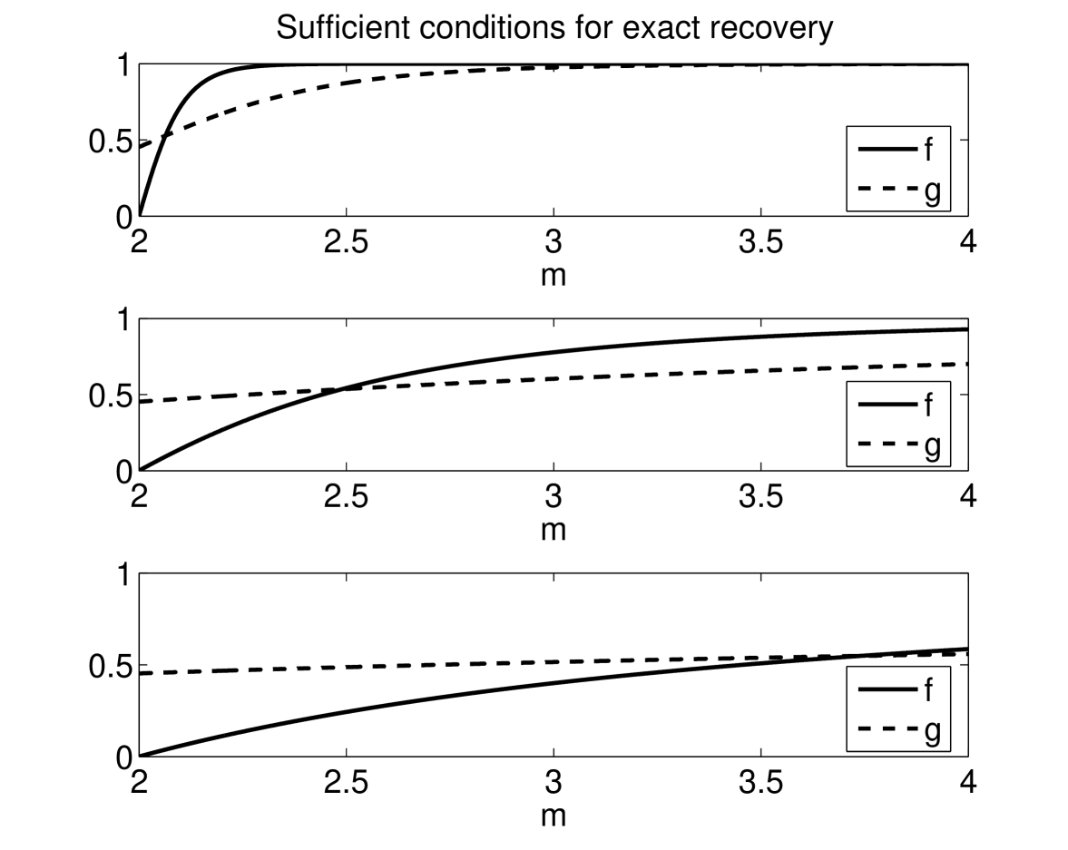
In [17], Foucart and Lai give different sufficient conditions for exact recovery than those we present. In particular, they show that if
| (16) |
holds for some , then will recover signals in exactly. Note that the sufficient condition in this paper, i.e., (12), holds when
| (17) |
for some . In Figure 1, we compare these different sufficient conditions as a function of for and respectively. Figure 1 indicates that neither sufficient condition is weaker than the other for all values of . In fact, we can deduce that (16) is weaker when is close to 2, while (17) is weaker when starts to grow larger. Since both conditions are only sufficient, if either one of them holds for an appropriate , then recovers all signals in .
Remark 13
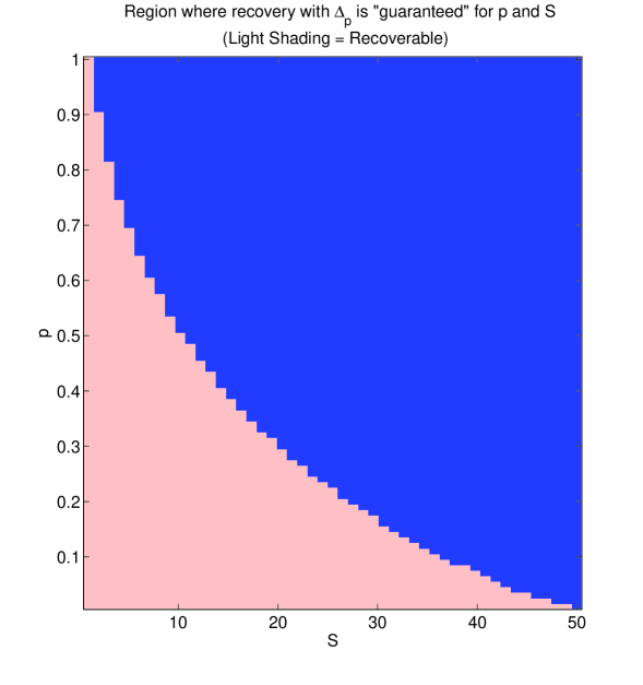
In [12], Davies and Gribonval showed that if one chooses (where can be computed implicitly for ), then there exist matrices (matrices in that correspond to tight Parseval frames in ) with the prescribed for which fails to recover signals in . Note that this result does not contradict with the results that we present in this paper: we provide sufficient conditions (e.g., (12)) in terms of , where and , that guarantee recovery by . These conditions are weaker than the corresponding conditions ensuring recovery by , which suggests that using can be beneficial. Moreover, the numerical examples we provide in Section 3 indicate that by using , , one can indeed recover signals in , even when fails to recover them (see Figure 2).
Remark 14
In summary, Theorem 6 states that if (12) is satisfied then we can recover signals in stably by decoding with . It is worth mentioning that the sufficient conditions presented here reduce the gap between the conditions for exact recovery with (i.e., ) and with , e.g., . For example for and , is sufficient. In the next subsection, we quantify this improvement.
2.2 The relationship between and
Let be an matrix and suppose , are its -restricted isometry constants. Define for with as the largest value of for which the slightly stronger version of (12) given by
| (18) |
holds for some , . Consequently, by Theorem 6, for all . We now establish a relationship between and .
Proposition 15
Suppose, in the above described setting, there exists and , such that
| (19) |
Then recovers all -sparse vectors, and recovers all sparse vectors with
Remark 16
For example, if then using , we can recover all -sparse vectors with .
2.3 Instance optimality in probability and
In this section, we show that is instance optimal in probability when is an appropriate random matrix. Our approach is based on that of [30], which we summarize now. A matrix is said to possess the property if and only if
where denotes the unit ball in . In [30], Wojtaszczyk shows that random Gaussian matrices of size as well as matrices whose columns are drawn uniformly from the sphere possess, with high probability, the property with . Noting that such matrices also satisfy with , again with high probability, Wojtaszczyk proves that , for these matrices, is (2,2) instance optimal in probability of order . Our strategy for generalizing this result to with relies on a generalization of the property to an property. Specifically, we say that a matrix satisfies if and only if
We first show that a random matrix , either Gaussian or uniform as mentioned above, satisfies the property with
Once we establish this property, the proof of instance optimality in probability for proceeds largely unchanged from Wojtaszczyk’s proof with modifications to account only for the non-convexity of the -quasinorm with .
Next, we present our results on instance optimality of the decoder, while deferring the proofs to Section 4. Throughout the rest of the paper, we focus on two classes of random matrices: denotes matrices, the entries of which are drawn from a zero mean, normalized column-variance Gaussian distribution, i.e., where ; in this case, we say that is an Gaussian random matrix. , on the other hand, denotes matrices, the columns of which are drawn uniformly from the sphere; in this case we say that is an uniform random matrix. In each case, denotes the associated probability space.
We start with a lemma (which generalizes an analogous result of [30]) that shows that the matrices and satisfy the property with high probability.
Lemma 17
Let , and let be an Gaussian random matrix. For , suppose that for some and some constants . Then, there exists a constant , independent of , , and , and a set
such that .
In other words, satisfies the , , with probability on the draw of the matrix. Here is a positive constant that depends only on . (In particular, and see (50) for the explicit value of when ). This statement is true also for .
The above lemma for can be found in [30]. As we will see in Section 4, the generalization of this result to is non-trivial and requires a result from [18], cf. [23], relating certain “distances” of -convex bodies to their convex hulls. It is important to note that this lemma provides the machinery needed to prove the following theorem, which extends to , , the analogous result of Wojtaszczyk [30] for .
In what follows, for a set , ; for , denotes the vector with entries for all , and for .
Theorem 18
Let . Suppose that satisfies and for some and as in (50). Let be an arbitrary decoder. If is (2,p) instance optimal of order with constant , then for any and , all of the following hold.
-
(i)
-
(ii)
-
(iii)
Above, denotes the set of indices of the largest (in magnitude) coefficients of ; the constants (all denoted by ) depend on , , , and but not on and . For the explicit values of these constants see (38) and (39).
Finally, our main theorem on the instance optimality in probability of the decoder follows.
Theorem 19
Let , and let be an Gaussian random matrix. Suppose that . There exists constants such that for all with , the following are true.
-
(i)
There exists with such that for all
(20) for any and for any .
-
(ii)
For any , there exists with such that for all
(21) for any .
The statement also holds for , i.e., for random matrices the columns of which are drawn independently from a uniform distribution on the sphere.
Remark 20
The constants above (both denoted by ) depend on the parameters of the particular and RIP properties that the matrix satisfies, and are given explicitly in Section 4, see (38) and (41). The constants , and depend only on and the distribution of the underlying random matrix (see the proof in Section 4.5) and are independent of and .
Remark 21
Clearly, the statements do not make sense if the hypothesis of the theorem forces to be 0. In turn, for a given pair, it is possible that there is no positive integer for which the conclusions of Theorem 19 hold. In particular, to get a non-trivial statement, one needs .
Remark 22
Note the difference in the order of the quantifiers between conclusions (i) and (ii) of Theorem 19. Specifically, with statement (i), once the matrix is drawn from the “good” set , we obtain the error guarantee (20) for every and . In other words, after the initial draw of a good matrix , stability and robustness in the sense of (20) are ensured. On the other hand, statement (ii) concludes that associated with every is a “good” set (possibly different for different ) such that if the matrix is drawn from , then stability and robustness in the sense of (21) are guaranteed. Thus, in (ii), for every , a different matrix is drawn, and with high probability on that draw (21) holds.
Remark 23
The above theorem pertains to the decoders which, like the analogous theorem for presented in [30], requires no knowledge of the noise level. In other words, provides estimates of sparse and compressible signals from limited and noisy observations without having to explicitly account for the noise in the decoding. This provides an improvement on Theorem 6 and a practical advantage when estimates of measurement noise levels are absent.
3 Numerical Experiments
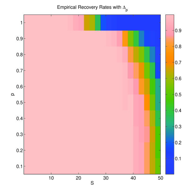
In this section, we present some numerical experiments to highlight important aspects of sparse reconstruction by decoding using , . First, we compare the sufficient conditions under which decoding with guarantees perfect recovery of signals in for different values of and . Next, we present numerical results illustrating the robustness and instance optimality of the decoder. Here, we wish to observe the linear growth of the reconstruction error , as a function of and of .
To that end, we generate a matrix whose columns are drawn from a Gaussian distribution and we estimate its RIP constants via Monte Carlo (MC) simulations. Under the assumption that the estimated constants are the correct ones (while in fact they are only lower bounds), Figure 2 (left) shows the regions where (12) guarantees recovery for different -pairs. On the other hand, Figure 2 (right) shows the empirical recovery rates via quasinorm minimization: To obtain this figure, for every , we chose 50 different instances of where non-zero coefficients of each were drawn i.i.d. from the standard Gaussian distribution. These vectors were encoded using the same measurement matrix as above. Since there is no known algorithm that will yield the global minimizer of the optimization problem (11), we approximated the action of by using a projected gradient algorithm on a sequence of smoothed versions of the minimization problem: In (11), instead of minimizing the , we minimized initially with a large . We then used the corresponding solution as the starting point of the next subproblem obtained by decreasing the value of according to the rule . We continued reducing the value of and solving the corresponding subproblem until becomes very small. Note that this approach is similar to the one described in [7]. The empirical results show that (in fact, the approximation of as described above) is successful in a wider range of scenarios than those predicted by Theorem 6. This can be attributed to the fact that the conditions presented in this paper are only sufficient, or to the fact that in practice what is observed is not necessarily a manifestation of uniform recovery. Rather, the practical results could be interpreted as success of with high probability on either or .
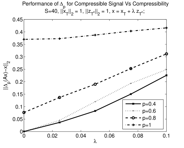
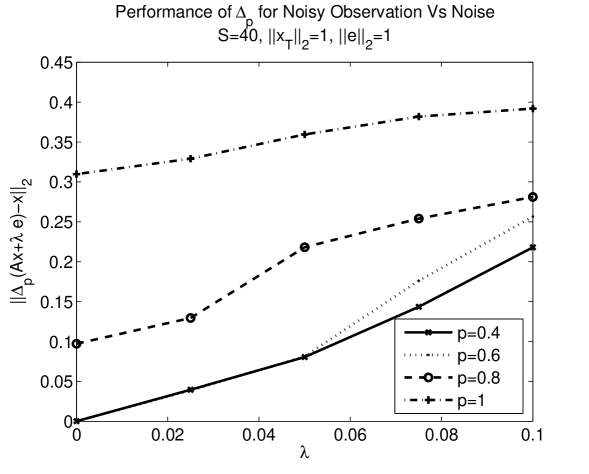
Next, we generate scenarios that allude to the conclusions of Theorem 19. To that end, we generate a signal composed of , supported on an index set , and a signal supported on , where all the coefficients are drawn from the standard Gaussian distribution. We then normalize and so that and generate with increasing values of (starting from 0), thereby increasing . For this experiment, we choose our measurement matrix by drawing its columns uniformly from the sphere. For each value of we measure the reconstruction error , and we repeat the process 10 times while randomizing the index set but preserving the coefficient values. We report the averaged results in Figure 3 (left) for different values of . Similarly, we generate noisy observations , of a sparse signal where and we increase the noise level starting from . Here, again, the non-zero entries of and all entries of were chosen i.i.d. from the standard Gaussian distribution and then the vectors were properly normalized. Next, we measure (for 10 realizations where we randomize ) and report the averaged results in Figure 3 (right) for different values of . In both these experiments, we observe that the error increases roughly linearly as we increase , i.e., and the noise power, respectively. Moreover, when the signal is highly compressible or when the noise level is low, we observe that reconstruction using with yields a lower approximation error than that with . It is also worth noting that for values of close to one, even in the case of sparse signals with no noise, the average reconstruction error is non-zero. This may be due to the fact that for such large the number of measurements is not sufficient for the recovery of signals with , further highlighting the benefits of using the decoder , with smaller values of .
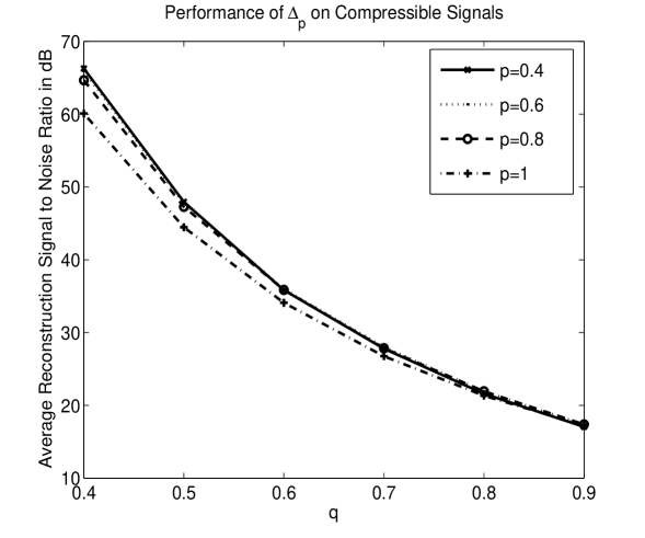
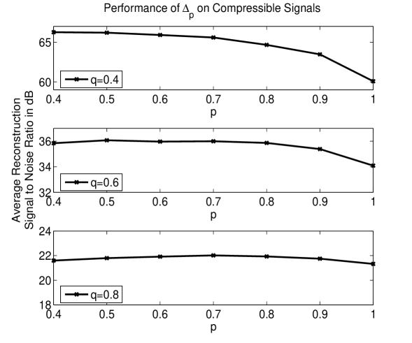
Finally, in Figure 4, we plot the results of an experiment in which we generate signals with sorted coefficients that decay according to some power law. In particular, for various values of , we set such that . We then encode with 50 different measurement matrices the columns of which were drawn from the uniform distribution on the sphere, and examine the approximations obtained by decoding with for different values of . The results indicate that values of provide the lowest reconstruction errors. Note that in Figure 4, we report the results in form of signal to noise ratios defined as
4 Proofs
4.1 Proof of Proposition 15
First, note that for any , is non-decreasing in . Also, the map is increasing in for .
Set
Then
We now describe how to choose and such that , , and (this will be sufficient to complete the proof using the monotonicity observations above). First, note that this last equality is satisfied only if is in the set
Let be such that
| (22) |
To see that such an exists, recall that where . Also, with , and . Consequently, , and . Thus, we know that we can find as above. Furthermore, . It follows from (22) that
We now choose
Then , and . So, we conclude that for as above and
we have
Consequently, the condition of Corollary 10 is satisfied and we have the desired conclusion. ∎
4.2 Proof of Theorem 6
We modify the proof of Candès et. al. of the analogous result for the encoder (Theorem 2 in [4]) to account for the non-convexity of the quasinorm. We give the full proof for completeness. We stick to the notation of [4] whenever possible.
Let , be arbitrary, and define and . Our goal is to obtain an upper bound on given that (by definition of ).
Below, for a set , ; for , denotes the vector with entries for all , and for .
( I ) We start by decomposing as a sum of sparse vectors with disjoint support. In particular, denote by the set of indices of the largest (in magnitude) coefficients of (here is to be determined later). Next, partition into sets , for where (also to be determined later), such that is the set of indices of the largest (in magnitude) coefficients of , is the set of indices of the second largest coefficients of , and so on. Finally let . We now obtain a lower bound for using the RIP constants of the matrix . In particular, we have
| (23) | |||||
Above, together with RIP, we used the fact that satisfies the triangle inequality for any . What now remains is to relate and to .
( II ) Next, we aim to bound from above in terms of . To that end, we proceed as in [4]. First, note that for all , and thus . It follows that , and consequently
| (24) |
Next, note that, similar to the case when as shown in [4], the “error” is concentrated on the “essential support” of (in our case ). To quantify this claim, we repeat the analogous calculation in [4]: Note, first, that by definition of ,
As satisfies the triangle inequality, we then have
Consequently,
| (25) |
which, together with (24), implies
| (26) |
where , and we used the fact that (which follows as ). Using (26) and (23), we obtain
| (27) |
where
| (28) |
At this point, using , we obtain an upper bound on given by
| (29) |
provided (this will impose the condition given in (12) on the RIP constants of the underlying matrix ).
( III ) To complete the proof, we will show that the error vector is concentrated on . Denote by the th largest (in magnitude) coefficient of and observe that . As , we then have
| (30) |
Here, the last inequality follows because for
Finally, we use (25) and (30) to conclude
| (31) | |||||
Above, we used the fact that , and that for any , and , .
4.3 Proof of Lemma 17.
( I ) The following result of Wojtaszczyk [30, Proposition 2.2] will be useful.
Proposition 24 ([30])
Let be an Gaussian random matrix, let , and suppose that for some and some constants . Then, there exists a constant , independent of and , and a set
such that
The above statement is true also for .
We will also use the following adaptation of [18, Lemma 2] for which we will first introduce some notation. Define a body to be a compact set containing the origin as an interior point and star shaped with respect to the origin [23]. Below, we use to denote the convex-hull of a body . For , we denote by the “distance” between and given by
Finally, we call a body -convex if for any , whenever such that .
Lemma 25
Let , and let be a -convex body in . If , then
where
We defer the proof of this lemma to the Appendix.
( II ) Note that . This follows because , which is equal to the largest column norm of , is 1 by construction. Thus, for ,
that is, , and so is well-defined. Next, by Proposition 24, we know that there exists with such that for all ,
| (33) |
From this point on, let . Then
and consequently
| (34) |
The next step is to note that and consequently
We can now invoke Lemma 25 to conclude that
| (35) |
Finally, by using (34), we find that
| (36) |
and consequently
| (37) |
In other words, the matrix has the property with the desired value of for every with . Here is as specified in Proposition 24.
To see that the same is true for , note that there exists a set with such that for all , , for every column of (this follows from RIP). Using this observation one can trace the above proof with minor modifications. ∎
4.4 Proof of Theorem 18.
We start with the following lemma, the proof of which for follows with very little modification from the analogous proof of Lemma 3.1 in [30] and shall be omitted.
Lemma 26
Let and suppose that satisfies and with . Then for every , there exists such that
Here, . Note that depends only on , and .
We now proceed to prove Theorem 18. Our proof follows the steps of [30] and differs in the handling of the non-convexity of the quasinorms for .
First, recall that satisfies and , so by Lemma 26, there exists such that , , and . Now, , and is instance optimal with constant . Thus,
and consequently
where in the third inequality we used the fact in any that quasinorm satisfies the inequality for all . So, we conclude
| (38) |
That is (i) holds with .
Next, we prove parts (ii) and (iii) of Theorem 18. As in the analogous proof of [30], Theorem 18 (ii) can be seen as a special case of Theorem 18 (iii), with . We therefore turn to proving (iii). Once again, by Lemma 26, there exists and in such that the following hold.
Here is the set of indices of the largest (in magnitude) coefficients of , and and are as in the proof of Theorem 6.
Similar to the previous part we can see that and by the hypothesis of instance optimality of , we have
Consequently observing that and using the triangle inequality,
| (39) |
That is (iii) holds with . By setting , one can see that this is the same constant associated with (ii). This concludes the proof of this theorem. ∎
4.5 Proof of Theorem 19.
First, we show that is instance optimal of order for an appropriate range of with high probability. One of the fundamental results in compressed sensing theory states that for any , there exists and with , all depending only on , such that , , satisfies for any . See, e.g., [6],[1], for the proof of this statement as well as for the explicit values of the constants. Now, choose such that . Then, with , and as above, for every and for every , the RIP constants of satisfy (18) (and hence (12)), with . Thus, by Corollary 9 is instance optimal of order with constant as in (15).
Now, set with such that (note that such a exists if and are sufficiently large). By the hypothesis of the theorem, and satisfy the hypothesis of the Lemma 17 with , , some , and an appropriate (determined by above). Because
by Lemma 17, there exists , such that for every , satisfies where . Consequently, set . Then, , for . Note that depends on , which is now a universal constant, and , which depends only on the distribution of (and in particular its concentration of measure properties, see [1]). Now, if , satisfies , thus , as well as . Therefore we can apply part (i) of Theorem 18 to get the first part of this theorem, i.e.,
| (40) |
Here is as in (38) with . To finish the proof of part (i), note that for , and .
To prove part (ii), first define as the support of the largest coefficients (in magnitude) of and . Now, note that for any there exists a set with for some universal constant , such that for all , (this follows from the concentration of measure property of Gaussian matrices, see, e.g., [1]). Define . Thus, where . Note that the dependencies of are identical to those of discussed above. Recall that for , satisfies both and . We can now apply part (iii) of Theorem 18 to obtain for
| (41) |
Above, the constant is as in (39). Once again, note that for , to finish the proof for any . ∎
5 Appendix: Proof of Lemma 25
In this section we provide the proof of Lemma 25 for the sake of completeness and also because we explicitly calculate the optimal constants involved. Let us first introduce some notation used in [18] and [23].
For a body , define its gauge functional by , and let , , be the smallest constant such that
Given a -convex body and a positive integer , define
Note that .
Finally, conforming with the notation used in [18] and [23], we define . Note that this should not cause confusion as we do not refer to the RIP constants throughout the rest of the paper. It can be shown by a result of [24] that , cf. [18, Lemma 1] for a proof.
We will need the following propositions.
Proposition 27 (sub-additivity of )
For the gauge functional associated with a -convex body , the following inequality holds for any .
| (42) |
[Proof.] Let and . If at least one of and is zero, then (42) holds trivially. (Note that, as is a body, if and only if .) So, we may assume that both and are strictly positive. Since is compact, it follows that and . Furthermore, is -convex, i.e., for all with , we have . In particular, choose and . This gives . Consequently, by the definition of the gauge functional . Finally, and . ∎
Proposition 28
.
[Proof.] Note that , and thus, by definition, is the smallest constant such that for every positive integer and for every choice of points ,
| (43) |
For , we can choose to be orthonormal. Consequently,
and thus, . On the other hand, let be an arbitrary positive integer, and suppose that . Then, it is easy to show that there exists a choice of signs , such that
Indeed, we will show this by induction. First, note that . Next, assume that there exists such that
Then (using parallelogram law),
Choosing accordingly, we get
which implies that . Using the fact that which we showed above, we conclude that . ∎
Proof of Lemma 25
We now present a proof of the more general form of Lemma 25 as stated in [18] and [23] (albeit for the Banach-Mazur distance in place of ). The proof is essentially as in [18], cf. [23], which in fact also works with the distance to establish an upper bound on the Banach-Mazur distance between a -convex body and a symmetric body.
Lemma 29
Let , , and let be a -convex body. Suppose that is a symmetric body with respect to the origin such that . Then
where .
[Proof.] Note that , and therefore is well-defined. Let and . Thus, . Let be a positive integer and let be a collection of points in . Then, and by the definition of , there is a choice of signs so that . Since is symmetric, we can assume that has . Now we can write
| (44) | |||||
where the first inequality uses the sub-additivity of and the fact that . Thus by taking the supremum in (44) over all possible ’s and dividing by , we obtain, for any ,
By applying this inequality for , we obtain the following inequality for any
| (45) |
Since , we now want to minimize the right hand side in (45) by choosing appropriately. To that end, define
and
Since for any , the best bound on is essentially given by , where . However, since is not necessarily an integer (which we require), we will instead use as a bound. Thus, we solve to obtain . By evaluating at , we obtain for every . In other words, for every , we have
| (46) |
On the other hand, if , then . However, this last bound is one of the summands in the right hand side of (45) with (which we provide a bound for in (46)). Consequently (46) holds for all . In particular, it holds for the value of which achieves the supremum of . Since , we obtain
| (47) |
Remark 30
In the previous step we utilize the fact that in the derivations above we can replace every and with and respectively, thus every and with and without changing (46). This allows us to pass from the bound on to without any problems.
Recalling the definitions of and , note the following inclusions:
| (48) |
Consequently and the inequality
| (49) |
follows from the definition of . Combining (49) and (47) we complete the proof with
∎ Finally, we choose above and , recall that (see Proposition 28), and obtain Lemma 25 as a corollary with
| (50) |
Acknowledgment
The authors would like to thank Michael Friedlander, Gilles Hennenfent, Felix Herrmann, and Ewout Van Den Berg for many fruitful discussions. This work was finalized during an AIM workshop. We thank the American Institute of Mathematics for its hospitality. Moreover, R. Saab thanks Rabab Ward for her immense support. The authors also thank the anonymous reviewers for their constructive comments which improved the paper significantly.
References
- [1] R. Baraniuk, M. Davenport, R. DeVore, M. Wakin, A simple proof of the restricted isometry property for random matrices, Constructive Approximation 28 (3) (2008) 253–263.
- [2] E. J. Candès, The restricted isometry property and its implications for compressed sensing, Comptes rendus-Mathématique 346 (9-10) (2008) 589–592.
- [3] E. J. Candès, J. Romberg, T. Tao, Robust uncertainty principles: exact signal reconstruction from highly incomplete frequency information, IEEE Transactions on Information Theory 52 (2006) 489–509.
- [4] E. J. Candès, J. Romberg, T. Tao, Stable signal recovery from incomplete and inaccurate measurements, Communications on Pure and Applied Mathematics 59 (2006) 1207–1223.
- [5] E. J. Candès, T. Tao, Decoding by linear programming., IEEE Transactions on Information Theory 51 (12) (2005) 489–509.
- [6] E. J. Candès, T. Tao, Near-optimal signal recovery from random projections: universal encoding strategies?, IEEE Transactions on Information Theory 52 (12) (2006) 5406–5425.
- [7] R. Chartrand, Exact reconstructions of sparse signals via nonconvex minimization, IEEE Signal Processing Letters 14 (10) (2007) 707–710.
- [8] R. Chartrand, V. Staneva, Restricted isometry properties and nonconvex compressive sensing, Inverse Problems 24 (035020).
-
[9]
S. Chen, D. Donoho, M. Saunders, Atomic decomposition by basis pursuit, SIAM
Journal on Scientific Computing 20 (1) (1999) 33–61.
URL citeseer.ist.psu.edu/chen98atomic.html - [10] A. Cohen, W. Dahmen, R. DeVore, Compressed sensing and best k-term approximation, Journal of the American Mathematical Society 22 (1) (2009) 211–231.
- [11] I. Daubechies, R. DeVore, M. Fornasier, S. Gunturk, Iteratively re-weighted least squares minimization for sparse recovery, Communications on Pure and Applied Mathematics (to appear).
- [12] M. Davies, R. Gribonval, Restricted Isometry Constants where sparse recovery can fail for , IEEE Transactions on Information Theory 55 (5) (2009) 2203–2214.
- [13] D. Donoho, Compressed sensing., IEEE Transactions on Information Theory 52 (4) (2006) 1289–1306.
- [14] D. Donoho, M. Elad, Optimally sparse representation in general (nonorthogonal) dictionaries via minimization, Proceedings of the National Academy of Sciences of the United States of America 100 (5) (2003) 2197–2202.
- [15] D. Donoho, X. Huo, Uncertainty principles and ideal atomic decomposition, IEEE Transactions on Information Theory 47 (2001) 2845–2862.
- [16] M. Figueiredo, R. Nowak, S. Wright, Gradient Projection for Sparse Reconstruction: Application to Compressed Sensing and Other Inverse Problems, IEEE Journal of Selected Topics in Signal Processing 1 (4) (2007) 586–597.
- [17] S. Foucart, M. Lai, Sparsest solutions of underdetermined linear systems via -minimization for , Applied and Computational Harmonic Analysis 26 (3) (2009) 395–407.
- [18] Y. Gordon, N. Kalton, Local structure theory for quasi-normed spaces, Bulletin des sciences mathématiques 118 (1994) 441–453.
- [19] R. Gribonval, R. M. Figueras i Ventura, P. Vandergheynst, A simple test to check the optimality of sparse signal approximations, in: IEEE International Conference on Acoustics, Speech and Signal Processing (ICASSP’05), vol. 5, 2005.
- [20] R. Gribonval, R. M. Figueras i Ventura, P. Vandergheynst, A simple test to check the optimality of sparse signal approximations, EURASIP Signal Processing, special issue on Sparse Approximations in Signal and Image Processing 86 (3) (2006) 496–510.
- [21] R. Gribonval, M. Nielsen, On the strong uniqueness of highly sparse expansions from redundant dictionaries, in: International Conference on Independent Component Analysis (ICA’04), LNCS, Springer-Verlag, Granada, Spain, 2004.
- [22] R. Gribonval, M. Nielsen, Highly sparse representations from dictionaries are unique and independent of the sparseness measure, Applied and Computational Harmonic Analysis 22 (3) (2007) 335–355.
- [23] O. Guedon, A. Litvak, Euclidean projections of p-convex body, GAFA, Lecture Notes in Math 1745 (2000) 95–108.
- [24] N. Peck, Banach-mazur distances and projections on p-convex spaces, Mathematische Zeitschrift 177 (1) (1981) 131–142.
- [25] R. Saab, R. Chartrand, O. Yilmaz, Stable sparse approximations via nonconvex optimization, in: IEEE International Conference on Acoustics, Speech and Signal Processing (ICASSP), 2008.
- [26] J. Tropp, Recovery of short, complex linear combinations via minimization, IEEE Transactions on Information Theory 51 (4) (2005) 1568–1570.
-
[27]
E. van den Berg, M. Friedlander, In pursuit of a root, UBC Computer Science
Technical Report TR-2007-16.
URL http://www.optimization-online.org/DB_FILE/2007/06/1708%.pdf - [28] P. Vandergheynst, P. Frossard, Efficient image representation by anisotropic refinement in matching pursuit, in: IEEE International Conference on Acoustics, Speech, and Signal Processing (ICASSP), vol. 3, 2001.
- [29] R. Ventura, P. Vandergheynst, P. Frossard, Low rate and scalable image coding with redundant representations, IEEE Transactions on Image Processing 15 (3) (2006) 726–739.
-
[30]
P. Wojtaszczyk, Stability and instance optimality for gaussian measurements in
compressed sensing, Foundations of Computational Mathematics (to appear).
URL http://dx.doi.org/10.1007/s10208-009-9046-4