Spatial and Spatio-Temporal Log-Gaussian Cox Processes: Extending the Geostatistical Paradigm
Abstract
In this paper we first describe the class of log-Gaussian Cox processes (LGCPs) as models for spatial and spatio-temporal point process data. We discuss inference, with a particular focus on the computational challenges of likelihood-based inference. We then demonstrate the usefulness of the LGCP by describing four applications: estimating the intensity surface of a spatial point process; investigating spatial segregation in a multi-type process; constructing spatially continuous maps of disease risk from spatially discrete data; and real-time health surveillance. We argue that problems of this kind fit naturally into the realm of geostatistics, which traditionally is defined as the study of spatially continuous processes using spatially discrete observations at a finite number of locations. We suggest that a more useful definition of geostatistics is by the class of scientific problems that it addresses, rather than by particular models or data formats.
doi:
10.1214/13-STS441keywords:
, , and
1 Introduction
Spatial statistics has been one of the most fertile areas for the development of statistical methodology during the second half of the twentieth century. A striking, if slightly contrived, illustration of the pace of this development is the contrast between the 90 pages of Bartlett (1975) and the 900 pages of Cressie (1991). Cressie’s book established a widely used classification of spatial statistics into three subareas: geostatistical data, lattice data, spatial patterns (meaning point patterns). Within this classification, geostatistical data consist of observed values of some phenomenon of interest associated with a set of spatial locations , where, in principle, each could have been any location within a designated spatial region . Lattice data consist of observed values associated with a fixed set of locations , that is, the phenomenon of interest exists only at those specific locations. Finally, in a spatial pattern the data are a set of spatial locations presumed to have been generated as a partial realisation of a point process that is itself the object of scientific interest. Almost 20 years later, Gelfand et al. (2010) used the same classification but with a different terminology focused more on the underlying process than on the extant data: continuous spatial variation, discrete spatial variation, and spatial point processes. With this process-based terminology in place, continuous spatial variation implies a stochastic process , discrete spatial variation implies only a finite-dimensional random variable, , and a point pattern implies a counting measure, .
In this paper, we argue first that the most important theoretical distinction within spatial statistics is between spatially continuous and spatially discrete stochastic processes, and second that most natural processes are spatially continuous and should be modelled accordingly. One consequence of this point of view is that in many applications, maintaining a one-to-one linkage between data formats (geostatistical, lattice, point pattern) and associated model classes (spatially continuous, spatially discrete, point process) is inappropriate. In particular, we suggest a redefinition of geostatistics as the collection of statistical models and methods whose purpose is to enable predictive inference about a spatially continuous, incompletely observed phenomenon, , say.
Classically, geostatistical data correspond to noisy versions of . A standard geostatistical model, expressed here in hierarchical form, is that is a Gaussian stochastic process, whilst conditional on , the are mutually independent, Normally distributed with means and common variance . A second scenario, and the focus of the current paper, is when determines the intensity, , say, of an observed Poisson point process. An example that we will consider in detail is a log-linear specification, , where is a Gaussian process. A third form is when the point process is reduced to observations of the numbers of points in each of regions that form a partition (or subset) of the region of interest . Hence, conditional on , the are mutually independent, Poisson-distributed with means
| (1) |
In the remainder of the paper we show how the log-Gaussian Cox process can be used in a range of applications where is incompletely observed through the lens of point pattern or aggregated count data. Sections 2 to 4 concern theoretical properties, inference and computation. Section 5 describes several applications. Section 6 discusses the extension to spatio-temporal data. Section 7 gives an outline of how this approach to modelling incompletely observed spatial phenomena extends naturally to the joint analysis of multivariate spatial data when the different data elements are observed at incommensurate spatial scales. Section 8 is a short, concluding discussion.
2 The Log-Gaussian Cox Process
A (univariate, spatial) Cox process (Cox (1955)) is a point process defined by the following two postulates: {longlist}[CP2:]
is a nonnegative-valued stochastic process;
conditional on the realisation , the point process is an inhomogeneous Poisson process with intensity .
Cox processes are natural models for point process phenomena that are environmentally driven, much less natural for phenomena driven primarily by interactions amongst the points. Examples of these two situations in an epidemiological context would be the spatial distribution of cases of a noninfectious or infectious disease, respectively. In a noninfectious disease, the observed spatial pattern of cases results from spatial variation in the exposure of susceptible individuals to a combination of observed and unobserved risk-factors. Conditional on exposure, cases occur independently. In contrast, in an infectious disease the observed pattern is at least partially the result of infectious cases transmitting the disease to nearby susceptibles. Notwithstanding this phenomenological distinction, it can be difficult, or even impossible, to distinguish empirically between processes representing stochastically independent variation in a heterogeneous environment and stochastic interactions in a homogeneous environment (Bartlett (1964)).
The moment properties of a Cox process are inherited from those of the process . For example, in the stationary case the intensity of the Cox process is equal to the expectation of and the covariance density of the Cox process is equal to the covariance function of . Hence, writing and , the reduced second moment measure or -function (Ripley 1976, 1977) of the Cox process is
| (2) |
Møller, Syversveen and Waagepetersen (1998) introduced the class of log-Gaussian processes(LGCPs). As the name implies, an LGCP is a Cox process with , where is a Gaussian process. This construction has an elegant simplicity. One of its attractive features is that the tractability of the multivariate Normal distribution carries over, to some extent, to the associated Cox process.
In the stationary case, let and . It follows from the moment properties of the log-Normal distribution that the associated LGCP has intensity and covariance density . This makes it both convenient and natural to re-parameterise the model as
| (3) |
where , so that and . This re-parameterisation gives a clean separation between first-order (mean value) and second-order (variation about the mean) properties. Hence, for example, if we wished to model a spatially varying intensity by including one or more spatially indexed explanatory variables , a natural first approach would be to retain the stationarity of but replace the constant intensity by a regression model, . The resulting Cox process is now an intensity-reweighted stationary point process (Baddeley, Møller and Waagepetersen, 2000), which is the analogue of a real-valued process with a spatially varying mean and a stationary residual.
The definition of a multivariate LGCP is immediate—we simply replace the scalar-valued Gaussian process by a vector-valued multivariate Gaussian process—and its moment properties are equally tractable. For example, if is a stationary bivariate Gaussian process with intensities and , and cross-covariance function , the cross-covariance density of the associated Cox process is .
There is an extensive literature on parametric specifications for the covariance structure of real-valued processes ; for a recent summary, see Gneiting and Guttorp (2010a). The theoretical requirement for a function to be a valid covariance function is that it be positive-definite, meaning that for all positive integers , any associated set of points , and any associated set of real numbers ,
| (4) |
Checking that (4) holds for an arbitrary candidate is not straightforward. In practice, we choose covariance functions from a catalogue of parametric families that are known to be valid. In the stationary case, a widely used family is the Matérn (1960) class , where
| (5) | |||
In (2), is the complete Gamma function, is a modified Bessel function of order , and and are parameters. The parameter has units of distance, whilst is a dimensionless shape parameter that determines the differentiability of the corresponding Gaussian process; specifically, the process is -times mean square differentiable if . This physical interpretation of is useful because is difficult to estimate empirically (Zhang (2004)), hence, a widely used strategy is to choose between a small set of values corresponding to different degrees of differentiability, for example, or . Estimation of is more straightforward.
In summary, the LGCP is the natural analogue for point process data of the linear Gaussian model for real-valued geostatistical data (Diggle and Ribeiro (2007)). Like the linear Gaussian model, it lacks any mechanistic interpretation. Its principal virtue is that it provides a flexible and relatively tractable class of empirical models for describing spatially correlated phenomena. This makes it extremely useful in a range of applications where the scientific focus is on spatial prediction rather than on testing mechanistic hypotheses. Section 5 gives several examples.
3 Inference for Log-Gaussian Cox Processes
In this section we distinguish between two inferential targets, namely, estimation of model parameters and prediction of the realisations of unobserved stochastic processes. Within the Bayesian paradigm, this distinction is often blurred, because parameters are treated as unobserved random variables and the formal machinery of inference is the same in both cases, consisting of the calculation of the conditional distribution of the target given the data. However, from a scientific perspective parameter estimation and prediction are fundamentally different, because the former concerns properties of the process being modelled whereas the latter concerns properties of a particular realisation of that process.
3.1 Parameter Estimation
For parameter estimation, we consider three approaches: moment-based estimation, maximum likelihood estimation, and Bayesian estimation. The first approach is typically very simple to implement and is useful for the initial exploration of candidate models. The second and third are more principled, both being likelihood-based.
3.1.1 Moment-based estimation
In the stationary case, moment-based estimation consists of minimising a measure of the discrepancy between empirical and theoretical second-moment properties. One class of such measures is a weighted least squares criterion,
| (6) |
In the intensity-re-weighted case, (6) can still be used after separately estimating a regression model for a spatially varying under the working assumption that the data are a partial realisation of an inhomogeneous Poisson process.
This method of estimation has an obviously ad hoc quality. In particular, it is difficult to give generally applicable guidance on appropriate choices for the values of and in (6). Because the method is intended only to give preliminary estimates, there is something to be said for simply matching and by eye. The R (R Core Team (2013)) package lgcp (Taylor et al., 2013) includes an interactive graphics function to facilitate this.
3.1.2 Maximum likelihood estimation
The general form of the Cox process likelihood associated with data is
where
| (8) |
is the likelihood for an inhomogeneous Poisson process with intensity . The evaluation of (3.1.2) involves integration over the infinite-dimensional distribution of . In Section 4.1 below we describe an implementation in which the continuous region of interest is approximated by a finely spaced regular lattice, hence replacing by a finite set of values , where the points cover . Even so, the high dimensionality of the implied integration appears to present a formidable obstacle to analytic progress. One solution, easily stated but hard to implement robustly and efficiently, is to use Monte Carlo methods.
Monte Carlo evaluation of (3.1.2) consists of approximating the expectation by an empirical average over simulated realisations of some kind. A crude Monte Carlo method would use the approximation
| (9) |
where are simulated realisations of on the set of grid-points . In practice, this is hopelessly inefficient. A better approach is to use an ingenious method due to Geyer (1999), as follows.
Let denote the un-normalised joint density of and . Then, the associated likelihood is
| (10) |
where
| (11) |
is the intractable normalising constant for . It follows that
| (12) | |||
where is any convenient, fixed value of , and denotes expectation when . However, the function in (10) is also an un-normalised conditional density for given . Under this second interpretation, the corresponding normalised conditional density is , where
| (13) |
and the same argument as before gives
| (14) | |||
It follows from (3.1.2), (10) and (13) that the likelihood for the observed data, , can be written as
| (15) |
Hence, the log-likelihood ratio between any two parameter values, and , is
| (16) | |||
Substitution from (3.1.2) and (3.1.2) gives the result that
| (17) | |||
where . For any fixed value of , a Monte Carlo approximation to the log-likelihood, ignoring the constant term on the left-hand side of (3.1.2), is therefore given by
The result (3.1.2) provides a Monte Carlo approximation to the log-likelihood function, and therefore to the maximum likelihood estimate , by simulating the process only at a single value, . The accuracy of the approximation depends on the number of simulations, , and on how close is to .
Note that in the second term on the right-hand side of (3.1.2) the pairs are simulated joint realisations of and at , whilst in the first term is held fixed at the observed data and the simulated realisations are conditional on . Conditional simulation of requires Markov chain Monte Carlo (MCMC) methods, for which careful tuning is generally needed. We discuss computational issues, including the design of a suitable MCMC algorithm, in Section 4.
3.1.3 Bayesian estimation
One way to implement Bayesian estimation would be directly to combine Monte Carlo evaluation of the likelihood with a prior for . However, it turns out to be more efficient to incorporate Bayesian estimation and prediction into a single MCMC algorithm, as described in Section 4.
3.2 Prediction
For prediction, we consider plug-in and Bayesian prediction. Suppose, quite generally, that data are to be used to predict a target under an assumed model with parameters . Then, plug-in prediction consists of a series of probability statements within the conditional distribution , where is a point estimate of , whereas Bayesian prediction replaces by
| (19) |
This shows that Bayesian prediction is a weighted average of plug-in predictions, with different values of weighted according to the Bayesian posterior for . The Bayesian solution (19) is the more correct in that it incorporates parameter uncertainty in a way that is both natural, albeit on its own terms, and elegant.
4 Computation
Inference for LGCPs is a computationally challenging problem. Throughout this section we will use the notation and language of purely spatial processes on , but the discussion applies in more general settings including spatio-temporal LGCPs.
4.1 The Computational Grid
Although we model the latent process as a spatially continuous process, in practice, we work with a piecewise-constant equivalent to the LGCP model on a collection of cells that form a disjoint partition of the region of interest, . In the limit as the number of cells tends to infinity, this process behaves like its spatially continuous counterpart. We call the collection of cells on which we represent the process the computational grid. The choice of grid reflects a balance between computational complexity and accuracy of approximation. The computational bottleneck arises through the need to invert the covariance matrix, , corresponding to the variance of evaluated on the computational grid.
Typically, we shall use a computational grid of square cells. This is an example of a regular grid, by which we mean that on an extension of the grid notionally wrapped on a torus, a strictly stationary covariance function of the process on will induce a block-circulant covariance structure on the grid (Wood and Chan (1994); Møller, Syversveen and Waagepetersen, 1998). For simplicity of presentation, we make no distinction between the extended grid and the original grid, since for extensions that at least double the width and height of the original grid, the toroidal distance between any two cells in the original observation window coincides with their Euclidean distance in . For a second-order stationary process , inversion of on a regular grid is best achieved using Fourier methods (Frigo and Johnson (2011)). On irregular grids, sparse matrix methods in conjunction with an assumption of low-order Markov dependence are more efficient (Rue and Held (2005); Rue, Martino and Chopin (2009); Lindgren, Rue and Lindström, 2011). In this context, Lindgren, Rue and Lindström (2011) demonstrate a link between models assuming a Markov dependence structure and spatially continuous models whose covariance function belongs to a restricted subset of the Matérn class.
4.2 Implementing Bayesian Inference, MCMC or INLA?
We now suppose that the computational grid has been defined and the point process data have been converted to a set of counts, , on the grid cells; note that we envisage using a finely spaced grid, for which cell-counts will typically be 0 or 1. Our goal is to use the data to make inferences about the latent process and the parameters and , which, respectively, parameterise the intensity of the LGCP and the covariance structure of .
In the Bayesian paradigm we treat , and as random variables, assign priors to the model parameters and make inferential statements using the posterior/predictive distribution,
Two options for computation are as follows: MCMC, which generates random samples from , and the integrated nested Laplace approximation (INLA), which uses a mathematical approximation.
Taylor and Diggle (2013a) compare the performance of MCMC and INLA for a spatial LGCP with constant expectation and parameters treated as known values. In this restricted scenario, they found that MCMC, run for 100,000 iterations, delivered more accurate estimates of predictive probabilities than INLA. However, they acknowledged that “further research is required in order to design better MCMC algorithms that also provide inference for the parameters of the latent field”.
Approximate methods such as INLA have the advantages that they produce results quickly and circumvent the need to assess the convergence and mixing properties of an MCMC algorithm. This makes INLA very convenient for quick comparisons amongst multiple candidate models, which would be a daunting task for MCMC. Against this, MCMC methods are more flexible in that extensions to standard classes of models can usually be accommodated with only a modest amount of coding effort. Also, an important consideration in some applications is that the currently available software implementation of INLA is limited to the evaluation of predictive distributions for univariate, or, at best, low-dimensional, components of the underlying model, whereas MCMC provides direct access to joint posterior/predictive distributions of nonlinear functions of the parameters and of the latent process . Mixing INLA and MCMC can therefore be a good overall computational strategy. For example, Haran and Tierney (2012) use a heavy-tailed approximation similar in spirit to INLA to construct efficient MCMC proposal schemes.
4.2.1 Markov Chain Monte Carlo inference for log-Gaussian Cox processes
MCMC methods generate samples from a Markov chain whose stationary distribution is the target of interest, in our case . Such samples are inherently dependent but, subject to careful checking of mixing and convergence properties, their empirical distribution is an unbiased estimate of the target, and, in principle, the associated Monte Carlo error can be made arbitrarily small by using a sufficiently long run of the chain. In the current context, we follow Møller, Syversveen and Waagepetersen (1998) and Brix and Diggle (2001) in using a standardised version of , denoted , and transform to the log-scale, so that the MCMC algorithm operates on the whole of , rather than on a restricted subset. We denote the th sample from the chain by and write for the target distribution.
The aim in designing MCMC algorithms for any specific class of problems is to achieve faster convergence and better mixing than would be obtained by generic off-the-shelf methods. Gilks, Richardson and Spiegelhalter (1995) and Gamerman and Lopes (2006) give overviews of the extensive literature on this topic. We focus our discussion on the Metropolis-Hastings (MH) algorithm, which includes as a special case the popular Gibbs sampler (Metropoliset al., 1953; Hastings (1970); Geman and Geman (1984); Spiegelhalter, Thomas and Best, 1999). In order to use the MH algorithm, we require a proposal density, . At the th iteration of the algorithm, we sample a candidate, , from , and set with probability
otherwise set . The choice of is critical. Previous research on inferential methods for spatial and spatio-temporal log-Gaussian Cox processes has advocated the Metropolis-adjusted Langevin algorithm (MALA), which mimics a Langevin diffusion on the target of interest; see Roberts and Tweedie (1996), Møller, Syversveen and Waagepetersen (1998) and Brix and Diggle (2001); note also Brix and Diggle (2003) and Taylor and Diggle (2013b). Alternatives to MH include Hamiltonian Monte Carlo methods, as discussed in Girolami and Calderhead (2011).
The Metropolis-adjusted Langevin algorithm exploits gradient information to identify efficient proposals. The algorithms in this article make use of a “pre-conditioning matrix”, (Girolami and Calderhead (2011)), to define the proposal
where is a scaling constant. Ideally, should be the negative inverse of the Fisher information matrix evaluated at the maximum likelihood estimate of , that is, where is the observed information. However, this matrix is massive, dense and intractable. In practice, we can obtain an efficient algorithm by choosing to be an approximation of and further by changing during the course of the algorithm using adaptive MCMC (Andrieu and Thoms (2008); Roberts and Rosenthal (2007)). In MALA algorithms, can be tuned adaptively to achieve an approximately optimal acceptance rate of 0.574 (Roberts and Rosenthal (2001)).
Since the gradient of with respect to can be both difficult to compute and computationally costly, we instead suggest a random walk proposal for the -component of . In the examples described in Section 5 we used the following overall proposal:
| (21) | |||
In (4.2.1), is an approximation to , and similarly for and . The constants , and are the approximately optimal scalings for Gaussian targets explored by the Gaussian random walk or MALA proposals (Roberts and Rosenthal (2001)); these are, respectively, , and , where is the dimension.
The acceptance rate for a random walk proposal is often tuned to around 0.234, which is optimal for a Gaussian target in the limit as the dimension of the target goes to infinity. At each step in our algorithm, we jointly propose new values for and for using, respectively, a MALA and a random walk component in the overall proposal, but we also seek to maintain an acceptance rate of 0.574 to achieve optimality for the MALA parts of the proposal. As a compromise, in our proposal we scale the matrix by a constant factor and the proposal covariance matrix by a single adaptive . In the examples described in Section 5 we used a value of , which appears to work well across a range of scenarios.
5 Applications
5.1 Smoothing a Spatial Point Pattern
The intensity, , of an inhomogeneous spatial point process is the unique nonnegative valued function such that the expected number of points of the process, called events, that fall within any spatial region is
| (22) |
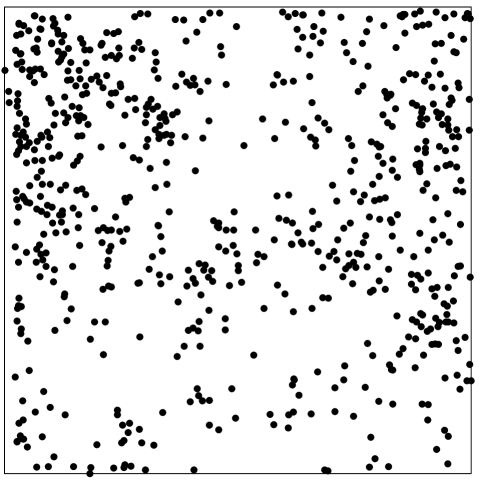
Suppose that we wish to estimate from a partial realisation consisting of all of the events of the process that fall within a region , hence, . Figure 1 shows an example in which the data are the locations of 703 hickory trees in a 19.6 acre (281.6 by 281.6 metre) square region (Gerrard (1969)), which we have re-scaled to be of dimension 100 by 100.
An intuitively reasonable class of estimators for is obtained by counting the number of events that lie within some fixed distance, , say, of and dividing by or, to allow for edge-effects, by the area, , of the intersection of and a circular disc with centre and radius , hence,
| (23) |
This estimate is, in essence, a simple form of bivariate kernel smoothing with a uniform kernel function (Silverman (1986)). Berman and Diggle (1989) derived the mean square error of (23) as a function of under the assumption that the underlying point process is a stationary Cox process. They then showed how to estimate, and thereby approximately minimise, the mean square error without further parametric assumptions.
A different way to formalise the smoothing problem is as a prediction problem associated with the log-Gaussian Cox process, (3). In this formulation, , where is a stationary Gaussian process indexed by a parameter and the target for prediction is . The formal solution is the predictive distribution of given . For a smooth estimate, analogous to (23), we take to be a suitable summary of the predictive distribution, for example, its point-wise expectation or median. This is still a nonparametric solution, in the sense that no parametric form is specified in advance for . The parameterisation of the Gaussian process is the counterpart of the choices made in the kernel estimation approach, namely, the specification of the uniform kernel in (23) and the value of the bandwidth, .
For this application, we specify that has mean , variance and exponential correlation function, , hence, . We conduct Bayesian predictive inference using MCMCmethods implemented in an extension of the R package lgcp (Taylor et al., 2013). For we chose a diffuse prior, . For and , we chose Normal priors on the log scale: and . We initialised theMCMC as follows. For and , we minimised
where is the -function of the model and is Ripley’s estimate (Ripley 1976, 1977), resulting in initial values of and . The initial value of was set to a matrix of zeros and was initialised using estimates from an overdispersed Poisson generalised linear model fitted to the cell counts, ignoring spatial correlation.
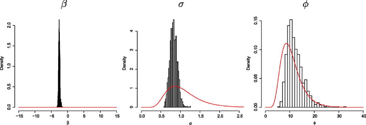
For the MCMC, we used a burn-in of 100,000 iterations followed by a further 900,000 iterations, of which we retained every 900th iteration so as to give a weakly dependent sample of size 1000. Convergence and mixing diagnostics are shown in the supplementary material [Diggle et al. (2013)]. Figure 2 compares the prior and posterior distributions of the three model parameters showing, in particular, that the data give only weak information about the correlation range parameter, . This is well known in the classical geostatistical context where the data are measured values of (see, e.g., Zhang (2004)), and is exacerbated in the point process setting.
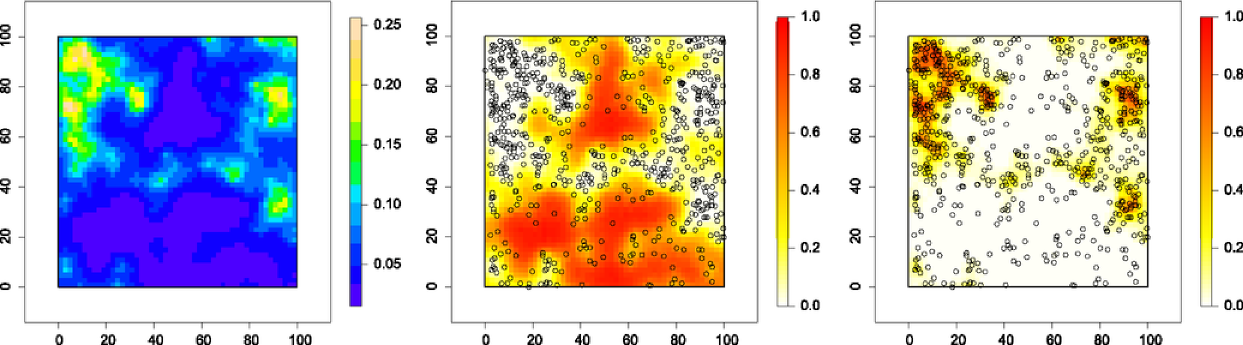
The left plot in Figure 3 shows the pointwise 50th percentiles of the predictive distribution for the target, over the observation window; this clearly identifies the pattern of the spatial variation in the intensity. The LGCP-based solution also enables us to map areas of particularly low or high intensity. The middle and right plots in Figure 3 are maps of and . The areas in these plots where the posterior probabilities are high correspond, respectively, to areas where the density of trees is less than half and more than double the mean density.
The LGCP-based solution to the smoothing problem is arguably over-elaborate by comparison with simpler methods such as kernel smoothing. Against this, arguments in its favour are that it provides a principled rather than an ad hoc solution, probabilistic prediction rather than point prediction, and an obvious extension to smoothing in the presence of explanatory variables by specifying , where is a vector of spatially referenced explanatory variables.
5.2 Spatial Segregation: Genotypic Diversity of Bovine Tuberculosis in Cornwall, UK
Our second application concerns a multivariate version of the smoothing problem described in Section 5.1. Events are now of types, hence, the data are , where and the corresponding intensity functions are . Write for the intensity of the superposition. Under the additional assumption that the underlying process is an inhomogeneous Poisson process, then conditional on the superposition, the labellings of the events are a sequence of independent multinomial trials with position-dependent multinomial probabilities,
| (24) |
A basic question for any multivariate point process data is whether the type-specific component processes are independent. When they are not, further questions of interest are context-specific. Here, we describe an analysis of data relating to bovine tuberculosis in the county of Cornwall, UK.
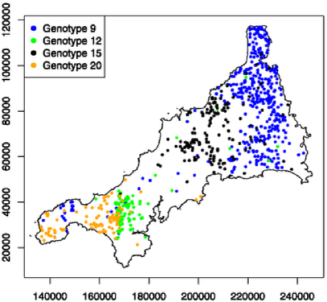
Bovine tuberculosis (BTB) is a serious disease of cattle. It is endemic in parts of the UK. As part of the national control strategy, herds are regularly inspected for BTB. When disease in a herd is detected and at least one tuberculosis bacterium is successfully cultured, the genotype that is responsible for the BTB breakdown can be determined. Here, we re-visit an example from Diggle, Zheng and Durr (2005) in which the events are the locations of cattle herds in the county of Cornwall, UK, that have tested positive for bovine BTB over the period 1989 to 2002, labelled according to their genotypes. The data, shown in Figure 4, are limited to the 873 locations with the four most common genotypes; six less common genotypes accounted for an additional 46 cases.
The question of primary interest in this example is whether the genotypes are randomly intermingled amongst the locations and, if not, to what extent specific genotypes are spatially segregated. This question is of interest because the former would be consistent with the major transmission mechanism being cross-infection during the county-wide movement of animals to and from markets, whereas the latter would be indicative of local pools of infection, possibly involving transmission between cattle and reservoirs of infection in local wildlife populations (Woodroffe et al., 2005; Donnelly et al. (2006)).
To model the data, we consider a multivariate log-Gaussian Cox process with
| (25) | |||
| (26) |
In (5.2), is the number of genotypes, the parameters relate to the intensities of the component processes, is a Gaussian process common to all types of points and the are Gaussian processes specific to each genotype. Although is not identifiable from our data without additional assumptions, its inclusion helps the interpretation of the model, in particular, by emphasising that the component intensities are not mutually independent processes.
In this example, we used informative priors for the model parameters: , and . Because the algorithm mixes slowly, this proved to be a very challenging computational problem. For the MCMC, we used a burn-in of 100,000 iterations followed by a further 18,000,000 iterations, of which we retained every 18,000th iteration so as to give a sample of size 1000. Convergence, mixing diagnostics and plots of the prior and posterior distributions of and are shown in the supplementary material [Diggle et al. (2013)]. These plots show that the chain appeared to have reached stationarity with low autocorrelation in the thinned output. The plots also illustrate that there is little information in the data on and .
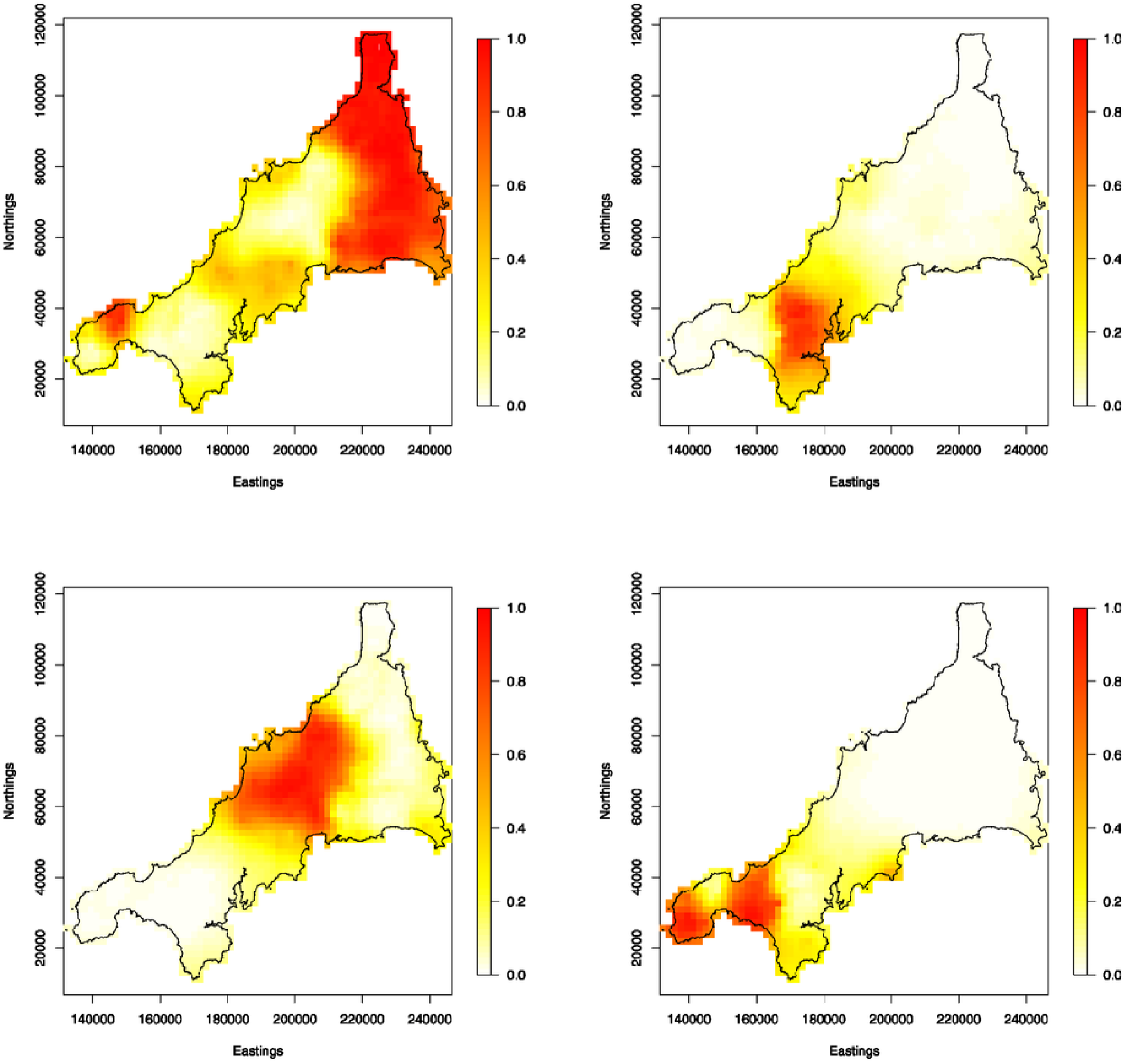
Within (5.2) the hypothesis of randomly intermingled genotypes corresponds to , for all . Were it the case that farms were uniformly distributed over Cornwall, would then represent the spatial variation in the overall risk of BTB, irrespective of genotype. Otherwise, conflates spatial variation in overall risk with the spatial distribution of farms. For the Cornwall BTB data the evidence against randomly intermingled genotypes is overwhelming and we focus our attention on spatial variation in the probability that a case at location is of type , for each of . These conditional probabilities are
and do not depend on the unidentifiable common component . Figure 5 shows point predictions of the four genotype-specific probability surfaces, defined as the conditional expectations for each of .
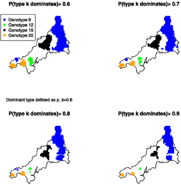
As argued earlier, one advantage of a model-based approach to spatial smoothing is that results can be presented in ways that acknowledge the uncertainty on the point predictions. We could replace each panel of Figure 5 by a set of percentile plots, as in Figure 3. For an alternative display that focuses more directly on the core issue of spatial segregation, let denote the set of locations for which . As and both approach 1, each shrinks towards the empty set, but more slowly in a highly segregated pattern than in a weakly segregated one. In Figure 6 we show the areas for each of and 0.9. Genotype 9, which contributes 494 to the total of 873 cases, dominates strongly in an area to the east and less strongly in a smaller area to the west. Genotype 15 contributes 166 cases and dominates in a single, central area. Genotypes 12 and 20 each contribute a proportion of approximately 0.12 to the total, with only small pockets of dominance to the south-west.
If infection times were known, we could perform inference via MCMC under a spatio-temporal version of the model,
| (27) |
with , and for spatio-temporal versions of the purely spatial processes in (5.2) and a vector of spatio-temporal covariates. Unlike purely spatial models, spatio-temporal models are potentially able to investigate mechanistic hypotheses about disease transmission. For example, in the context of this example a spatio-temporal analysis could distinguish between segregated patches that are stable over time or that grow from initially isolated cases.
5.3 Disease Atlases
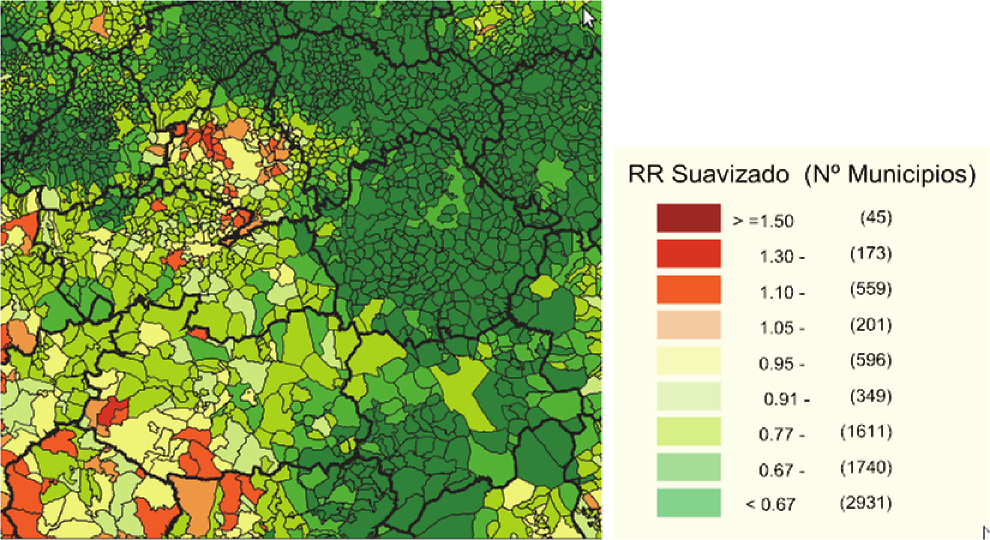
Figure 7 is a typical example of the kind of map that appears in a variety of cancer atlases. This example is taken from a Spanish national disease atlas project (López-Abente et al., 2006). The map estimates the spatial variation in the relative risk of lung cancer in the Castile-La Mancha Region of Spain and some surrounding areas. It is of a type known to geographers as a choropleth map, in which the geographical region of interest, , is partitioned into a set of subregions and each subregion is colour-coded according to the numerical value of the quantity of interest. The standard statistical methodology used to convert data on case-counts and the number of people at risk in each subregion is the following hierarchical Poisson-Gaussian Markov random field model, due to Besag, York and Molié (1991).
Let denote the number of cases in subregion and a standardised expectation computed as the expected number of cases, taking into account the demographics of the population in subregion but assuming that risk is otherwise spatially homogeneous. Assume that the are conditionally independent Poisson-distributed conditional on a latent random vector , with conditional means . Finally, assume that is multivariate Gaussian, with its distribution specified as a Gaussian Markov random field (Rue and Held (2005)). A Markov random field is a multivariate distribution specified indirectly by its full conditionals, . In the Besag, York and Molié (1991) model the full conditionals take the so-called intrinsic autoregressive form,
| (28) |
where is the mean of the over subregions considered to be neighbours of and is the number of such neighbours. Typically, subregions are defined to be neighbours if they share a common boundary.
An alternative approach is to model the locations of individual cancer cases as an LGCP with intensity , where represents population density, assumed known, and denotes disease risk, . Conditional on , case-counts in subregions are independent and Poisson-distributed with means
This approach leads to spatially smooth risk-maps whose interpretation is independent of the particular partition of into subregions . This is an important consideration when the differ greatly in size and shape, as the definition of neighbours in an MRF model then becomes problematic; see, for example, Wall (2004). Fitting a spatially continuous model also has the potential to add information to an analysis of aggregated data, for example, when data on environmental risk-factors are available at high spatial resolution. A caveat is that the population density may only be available in the form of small-area population counts, implying a piece-wise constant surface that can only be a convenient fiction. Note, however, that spatially continuous modelled population density maps have been constructed and are freely available; see, forexample, http://sedac.ciesin.columbia.edu/data/set/gpw-v3-population-density.
For the Spanish lung cancer data, we have covariate information available at small-area, which we incorporate by fitting the model
| (29) |
treating the covariate surfaces as piece-wise constant.
For Bayesian inference under the continuous model (29) we follow Li et al. (2012) by adding standard data augmentation techniques to the MCMC fitting algorithm described earlier. Recall that for computational purposes, we perform all calculations on a fine grid, treating the cell counts in each grid cell as Poisson distributed conditional on the latent process . Provided the computational grid is fine enough, each can be approximated by the union of a set of grid cells, and we can use a grid-based Gibbs sampling strategy, repeatedly sampling first from and then from , where are the cell counts on the computational grid, and parameterises the covariance structure of . Sampling from the first of these densities can be achieved using a Metropolis-Hastings update as discussed in Section 4. The second density is a multinomial distribution and poses no difficulty.
Our priors for this example were as follows: , and . For the MCMC algorithm, we used a burn-in of 100,000 iterations followed by a further 18,000,000 iterations, of which we retained every 18,000th iteration so as to give a sample of size 1000. Convergence, mixing diagnostics and plots of the prior and posterior distributions of and are shown in the supplementary material [Diggle et al. (2013)]. As in the Cornwall BTB analysis, these plots indicated convergence to the stationary distribution and low autocorrelation in the thinned output.
In the analysis reported here, we base our offset on modelled population data at 100 metre resolution obtained from the European Environment Agency; see http://www.eea.europa.eu/data-and-maps/data/population-density-disaggregated-with-corine-land-cover-2000-2. We projected this very fine population information onto our computational grid, which consisted of cells metres in dimension. We used an exponential model for the covariance function of and estimated its parameters (posterior median and 95% credible interval) to be and metres. Figure 8 illustrates the shape of the posterior covariance function; it can be seen from this plot that the posterior dependence between cells is over a relatively small range.
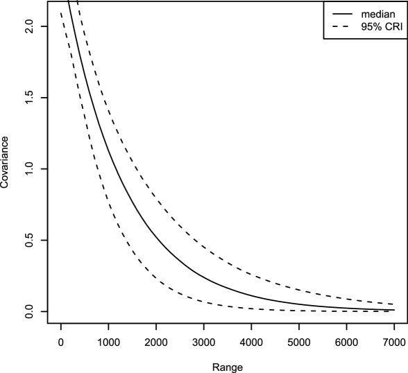
Table 1 summarises our estimation of covariate effects. Our results show that estimated (posterior median) mortality rates were higher in areas with higher rates of illiteracy and higher income; these effects were statistically significant at the 5% level, in the sense that the Bayesian 95% credible intervals excluded zero. The remaining covariates (unemployment, percentage farmers, percentage of people over 65 and average number of people per home) had a protective effect, but only significantly so in the case of percentage farmers.
| Quantile | |||
|---|---|---|---|
| Parameter | 0.50 | 0.025 | 0.975 |
| Percentage illiterate | 1.13 | 1.03 | 1.24 |
| Percentage unemployed | 0.92 | 0.8 | 1.03 |
| Percentage farmers | 0.88 | 0.76 | 1.00 |
| Percentage of people over 65 years old | 1.2 | 0.96 | 1.51 |
| Income index | 1.19 | 1.03 | 1.39 |
| Average number of people per home | 0.98 | 0.75 | 1.26 |
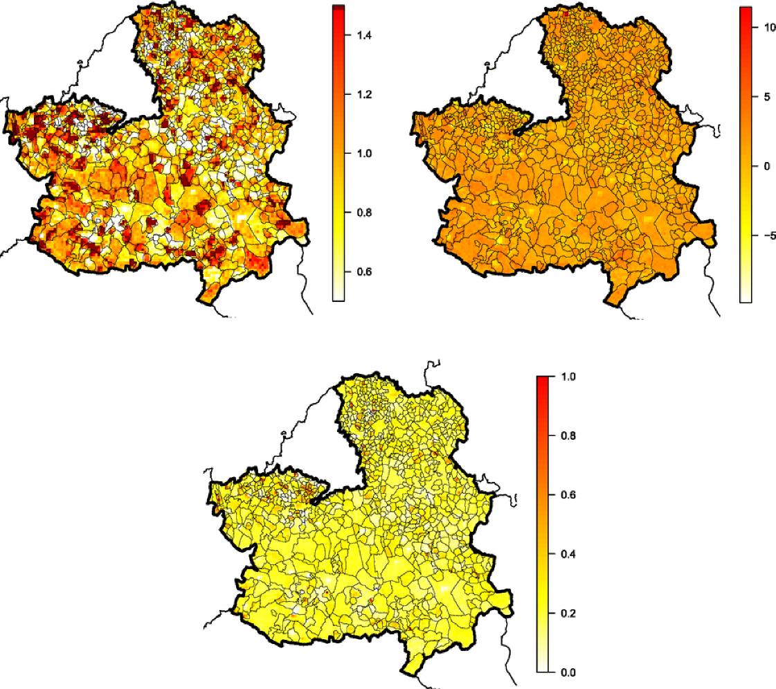
Figure 9 shows the resulting maps. The top left-hand panel shows the predicted, covariate-adjusted relative risk surface derived from the log-Gaussian Cox process model (29). This predicted relative risk surface reveals several small areas of raised risk that are not apparent in Figure 7. The top right-hand panel shows the log of the estimated variance of relative risk. To account for this variation, we produced a plot of the posterior probability that relative risk exceeds 1.1, shown in the bottom panel. This shows that higher rates of incidence appear to be mainly confined to a number of small townships, the largest of which is an area to the north of Toledo and surrounding the Illescas municipality, where there are a number of contiguous cells for which the probability exceeds 0.6.
We acknowledge that this is an illustrative example. In particular, we cannot guarantee the reliability of the estimate of population density used as an offset.
In a discussion of Markov models for spatial data, Wall (2004) investigated properties of the covariance structure implied by the simultaneous and conditional autoregressive models on an irregular lattice. She concluded that the “implied spatial correlation [between cells in these] models does not seem to follow an intuitive or practical scheme” and advises “[using] other ways of modelling lattice data should be considered, especially when there is interest in understanding the spatial structure”. Our approach is one such. Others, which we discuss in Section 7, include proposals in Best, Ickstadt and Wolpert (2000) and Kelsall and Wakefield (2002).
Our spatially continuous formulation does not entirely rescue us from the trap of the ecological fallacy (Piantadosi, Byar and Green, 1988; Greenland and Morgenstern (1990)). In a spatial context, this refers to the fact that the association between a risk-factor and a health outcome need not be, and usually is not, independent of the spatial scale on which the risk-factor and outcome variables are defined. In our example, we have to accept that treating covariate surfaces as if they were piece-wise constant is a convenient fiction. However, our methodology avoids any necessity to aggregate all covariate and outcome variables to a common set of spatial units, but rather operates at the fine resolution of the computational grid. In effect, this enables us to place a spatially continuous interpretation on any parameters relating to continuously measured components of the model, whether covariates or the latent stochastic process .
6 Spatio-Temporal Log-Gaussian Cox Processes
6.1 Models
A spatio-temporal LGCP is defined in the obvious way, as a spatio-temporal Poisson point process conditional on the realisation of a stochastic intensity function , where is a Gaussian process. Gneiting and Guttorp (2010b) review the literature on formulating models for spatio-temporal Gaussian processes. They make a useful distinction between physically motivated constructions and more empirical formulations. An example of the former is given in Brown et al. (2000), who propose models based on a physical dispersion process. In discrete time, with denoting the time-separation between successive realisations of the spatial field, their model takes the form
| (30) | |||
where is a smoothing kernel and is a noise process, in each case with parameters that depend on the value of in such a way as to give a consistent interpretation in the spatio-temporally continuous limit as .
Amongst empirical spatio-temporal covariancemodels, a basic distinction is between separable and nonseparable models. Suppose that is stationary, with variance and correlation function . In a separable model, , where and are spatial and temporal correlation functions. The separability assumption is convenient, not least because any valid specification of and guarantees the validity of , but it is not especially natural. Parametric families of nonseparable models are discussed in Cressie and Huang (1999), Gneiting (2002), Ma (2003, 2008) and Rodrigues and Diggle (2010).
As noted by Gneiting and Guttorp (2010b), whilst spatio-temporally continuous processes are, in formal mathematical terms, simply spatially continuous processes with an extra dimension, from a scientific perspective models need to reflect the fundamentally different nature of space and time, and, in particular, time’s directional quality. For this reason, in applications where data arise as a set of spatially indexed time-series, a natural way to formulate a spatio-temporal model is as a multivariate time series whose cross-covariance functions are spatially structured. For example, a spatially discrete version of (6.1) on a finite set of spatial locations and integer times would be
| (31) |
where the are functions of the corresponding locations, and . For a review of models of this kind, see Gamerman (2010).
6.2 Spatio-Temporal Prediction: Real-Time Monitoring of Gastrointestinal Disease
An early implementation of spatio-temporal log-Gaussian process modelling was used in the AEGISS project (Ascertainment and Enhancement ofGastroenteric Infection Surveillance Statistics, seehttp://www.maths.lancs.ac.uk/~diggle/Aegiss/day.html%3fyear=2002). The overall aim of the project was to investigate how health-care data routinely collected within the UK’s National Health Service (NHS) could be used to spot outbreaks of gastro-intestinal disease. The project is described in detail in Diggle et al. (2003), whilst Diggle, Rowlingson and Su (2005) give details of the spatio-temporal statistical model.
As part of the government’s modernisationprogramme for the NHS, the nonemergency NHS Direct telephone service was launched in the late 1990s, and by 2000 was serving all of Englandand Wales (http://www.nhsdirect.nhs.uk/About/WhatIsNHSDirect/History). Callers to this 24-hour system were questioned about their problem and advised accordingly. This process reduced calls to an “algorithm code” which was a broad classification of the problem. Basic information on the caller, including age, sex and postal code, was also recorded. Cooper and Chinemana (2004) give a more detailed description of the NHS Direct system. Mark and Shepherd (2004) analyse its impact on the demand for primary care in the UK. Cooper et al. (2003) report a retrospective analysis of 150,000 calls to NHS Direct classified as diarrhoea or vomiting, and concluded that fluctuations in the rate of such calls could be a useful proxy for monitoring the incidence of gastrointestinal illness.
In the AEGISS project, residential postal codes associated with calls classified as relating to diarrhoea or vomiting were converted to grid references using a lookup table. Postal codes at this level are referenced to 100 metre precision, which on the scale of the study area (the county of Hampshire) is effectively continuous. The data then formed a spatio-temporal point pattern.
The daily extraction of data for Hampshire and the location coding was done by the NHS at Southampton. These data were encrypted and sent by email to Lancaster, where the emails were automatically filtered, decrypted and stored. An overnight run of the MALA algorithm described in Brix and Diggle (2001) took the latest data and produced maps of predictive probabilities for the risk exceeding multiples 2, 4 and 8 of the baseline rate.
The specification of the model, based on an exploratory analysis of the data, was a spatio-temporal LGCP with intensity
The spatial baseline component, , was calculated by a kernel smoothing of the first two years of case locations, whilst the temporal baseline, , was obtained by fitting a standard Poisson regression model to the counts over time. This regression model included an annual seasonal component, a factor representing the day-of-the-week and a trend term to represent the increasing take-up of the NHS Direct service during the life-time of the project.
The parameters of were then estimated using moment-based methods, as in Brix and Diggle (2001), with a separable correlation structure. Uncertainty in these parameter estimates was considered to have a minimal effect on the predictive distribution of because parameter estimates are informed by all of the data, whereas prediction of given the model parameters benefits only from data points that lie close to , that is, within the range of the spatio-temporal correlation.
Plug-in predictive inference was then performed using the MALA algorithm on each new set of data arriving overnight. Instead of storing the outputs from each of 10,000 iterations, only a count of where exceeded a threshold that corresponded to 2, 4 or 8 times the baseline risk was retained. This range of thresholds was chosen in consultation with clinicians; a doubling of risk was considered of possible interest, whilst an eightfold increase was considered potentially serious. These exceedence counts were then converted into exceedence probabilities.
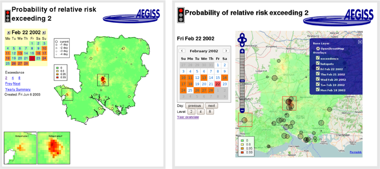
Presentation of these exceedence maps was an important aspect of the AEGISS project. At the time, there were few implementations of maps on the internet—UMN MapServer was released as open source in 1997 and the Google Maps service started in 2005. A simpler approach was used where static images of the exceedence probabilities were generated by R’s graphics system. Regions where the exceedence probability was higher than 0.9 were outlined with a box and displayed in a zoomed-in version below the main graphic. Other page controls enabled the user to select the threshold value as 2, 4 or 8, and to select a day or month. A traffic light system of green, amber and red warnings dependent on the severity of exceedence threshold crossings was developed for rapid assessment of conditions on any particular day. The left-hand panel of Figure 10 shows a day where two clusters of grid cells show high predictive probability of at least a doubling of risk relative to baseline.
With modern web-based technologies the user interface could be constructed as a dynamic web-mapping system that would allow the user freely to navigate the study region. Layers of information, such as cases or exceedence probability maps, can then be selected by the user as overlays. The right-hand panel of Figure 10 shows the same day as the left-hand panel, but uses the OpenLayers (http:// www.openlayers.org) web-mapping toolkit to superimpose the cases and risk surface on a base map composed of data from OpenStreetMap (http://www.openstreetmap.org). This also shows the layer selector menu for further customisation.
Increases in computing power and algorithmic advances mean that longer MCMC runs can be performed overnight or on finer spatial resolutions. However, increasing ethical concerns over data use and patient confidentiality mean that finely resolvedspatio-temporal data are becoming harder to obtain. Recent changes in the organisation of the NHS 24-hour telephone helpline has meant that several providers will now be responsible for regional services contributing to a new system, NHS111 (http:// www.nhs.uk/111). AEGISS was originally conceived as a pilot project that could be rolled out to all of the UK, but obtaining data from all the new providers and dealing with possible systematic differences between them in order to perform a statistically rigorous analysis is now more challenging. The future of health surveillance systems may lie in the use of multivariate spatio-temporal models to combine information from multiple data streams including nontraditional proxies for health outcomes, such as nonprescription medicine sales, counts of key words and phrases used in search engine queries, and text-mining of social media sites.
7 Data Synthesis: Integrated Analysis of Exposure and Health Outcome Data at Multiple Spatial Scales
The ubiquitous problem of dealing with exposure and health outcome data recorded at disparate spatial scales is known to geographers as the “modifiable areal unit problem.” See, for example, the reviews by Gotway and Young (2002) and Dark and Bram (2007). In the statistical literature, a more common term is “spatial misalignment.” See, for example, Gelfand (2010). Several authors have considered special cases of this problem in an epidemiological setting. Mugglin, Carlin and Gelfand (2000) deal with data in the form of disease counts on a partition of the region of interest, , into a discrete set of subregions, , together with covariate information on a different partition, , say. Their solution is based on creating a single, finer partition that includes all nonzero intersections . Best, Ickstadt and Wolpert (2000) also consider count data on a discrete partition of , but assume that covariate information on a risk factor of interest is available throughout . They consider count data to be derived from an underlying Cox process whose intensity varies in a spatially continuous manner through the combination of a covariate effect and a latent stochastic process modelled as a kernel-smoothed gamma random field. They then derive the distribution of the observed counts by spatial integration over the . Kelsall and Wakefield (2002) take a similar approach, but using a log-Gaussian latent stochastic process rather than a gamma random field. The technical and computational issues that arise when handling spatial integrals of stochastic processes can be simplified by using low-rank models, such as the class of Gaussian predictive process models proposed by Banerjee et al. (2008) and further developed by Finley et al. (2009). Gelfand (2012) gives a useful summary of this and related work.
All of these approaches can be subsumed within a single modelling framework for multiple exposures and disease risk by considering these as a set of spatially continuous processes, irrespective of the spatial resolution at which data elements are recorded. For example, a model for the spatial association between disease risk, , and exposures can be obtained by treating individual case-locations as an LGCP with intensity
| (32) |
where denotes stochastic variation in risk that is not captured by the covariate processes . The inferential algorithms associated with model (32) would then depend on the structure of the available data.
Suppose, for example, that health outcome data are available in the form of area-level counts, , in subregions , whilst exposure data are obtained as collections of unbiased estimates, , of the at corresponding locations . Suppose further that the are conditionally independent, with , the processes are jointly Gaussian and the process is also Gaussian and independent of the . A possible inferential goal is to evaluate the predictive distribution of the risk surface given the data and . In an obvious shorthand, and temporarily ignoring the issue of parameter estimation, the required predictive distribution is . The joint distribution of , , and factorises as
| (33) |
where and are multivariate Gaussian densities, is a product of univariate Gaussian densities, and is a product of Poisson probability distributions with means
Sampling from the required predictive distributions can then proceed using a suitable MCMC algorithm. For Bayesian parameter estimation, we would augment (33) by a suitable joint prior for the model parameters before designing the MCMC algorithm.
A specific example of data synthesis concerns an ongoing leptospirosis cohort study in a poor community within the city of Salvador, Brazil. Leptospirosis is considered to be the most widespread of the zoonotic diseases. This is due to the large number of people worldwide, but especially in poor communities, who live in close proximity to wild and domestic mammals that serve as reservoirs of infection and shed the agent in their urine. The major mode of transmission is contact with contaminated water or soil (Levett (2001); Bharti et al. (2003); McBride et al., 2005). In the majority of cases infection leads to an asymptomatic or mild, self-limiting febrile illness. However, severe cases can lead to potentially fatal acute renal failure and pulmonary haemorrhage syndrome. Leptospirosis is traditionally associated with rural-based subsistencefarming communities, but rapid urbanization and widening social inequality have led to the dramatic growth of urban slums, where the lack of basic sanitation favours rat-borne transmission (Ko et al., 1999; Johnson et al., 2004).
The goals of the cohort study are to investigate the combined effects of social and physical environmental factors on disease risk, and to map the unexplained spatio-temporal variation in incidence. In the study, approximately 1700 subjects at residential locations provide blood-samples on recruitment and at subsequent times approximately 6, 12, 18 and 24 months later. At each post-recruitment visit, sero-conversion is defined as achange from zero to positive, or at least a fourfold increase in concentration. The resulting data consist of binary responses, (sero-conversion no/yes), together with a mix of time-constant and time-varying risk-factors, .
A conventional analysis might treat the data from each subject as a time-sequence of binary responses with associated explanatory variables. Widely used methods for data of this kind include generalised estimating equations (Liang and Zeger (1986)) and generalised linear mixed models (Breslow and Clayton (1993)). An analysis more in keeping with the philosophy of the current paper would proceed as follows.
Let and denote time-constant and time-varying explanatory variables associated with subject , and the times at which blood samples are taken, setting for all . Note that explanatory variables can be of two distinct kinds: characteristics of an individual subject, for example, their age; and characteristics of a subject’s place of residence, for example, its proximity to an open-sewer. In principle, the latter can be indexed by a spatially continuous location, hence, and . A response indicates that at least one infection event has occurred in the time-interval . A model for each subject’s risk of infection then requires the specification of a set of person-specific hazard functions, . A model that allows for unmeasured risk factors would be a set of LGCPs, one for each subject, with respective stochastic intensities,
| (34) |
where the are mutually independent and is a spatio-temporally continuous Gaussian process. It follows that
| (35) | |||
In practice, values of and may only be observed incompletely, either at a finite number of locations or as small-area averages. For notational convenience, we consider only a single, incompletely observed spatio-temporal covariate whose measured values, , we model as
| (36) |
where is a spatio-temporal Gaussian process and the are mutually independent measurement errors. Then, (34) becomes
| (37) |
Inference for the model defined by (7), (36) and (37), based on data and , would require further development of MCMC algorithms of the kind de-scribed in Section 4.
8 Discussion
In this paper we have argued that the LGCP provides a useful class of models, not only for point process data but also for any problem involving prediction of an incompletely observed spatial or spatio-temporal process, irrespective of data format. Developments in statistical computation have made the combination of likelihood-based, classical or Bayesian parameter estimation and probabilistic prediction feasible for relatively large data sets, including real-time updating of spatio-temporal predictions.
In each of our applications, the focus has been on prediction of the spatial or spatio-temporal variation in a response surface, rather than on estimation of model parameters. In problems of this kind, where parameters are not of direct interest but rather are a means to an end, Bayesian prediction in conjunction with diffuse priors is an attractive strategy, as its predictions naturally accommodate the effect of parameter uncertainty. Model-based predictions are essentially nonparametric smoothers, but embedded within a probabilistic framework. This encourages the user to present results in a way that emphasises, rather than hides, their inherent imprecision.
In many public health settings, identifying where and when a particular phenomenon, such as disease incidence, is likely to have exceeded an agreed intervention threshold is more useful than quoting either a point estimate and its standard error or the statistical significance of departure from a benchmark.
The log-linear formulation is convenient because of the tractable moment properties of the log-Gaussian distribution. It also gives the model a natural interpretation as a multiplicative decomposition of the overall intensity into deterministic and stochastic components. However, it can lead to very highly skewed marginal distributions, with large patches of near-zero intensity interspersed with sharp peaks. Within the Monte Carlo inferential framework, there is no reason why other, less severe transformations from to should not be used.
Two areas of current methodological research are the formulation of models and methods for principled analysis of multiple data streams that include data of variable quality from nontraditional sources, and the further development of robust computational algorithms that can deliver reliable inferences for problems of ever-increasing complexity.
Our general approach reflects a continuing trend in applied statistics since the 1980s. The explosion in the development of computationally intensive methods and associated complex stochastic models has encouraged a move away from a methods-based classification of the statistics discipline and towards a multidisciplinary, problem-based focus in which statistical method (singular) is thoroughly embedded within scientific method.
Acknowledgements
We thank the Department of Environmental and Cancer Epidemiology in the National Center For Epidemiology (Spain) for providing aggregated data from the Castile-La Mancha region for permission to use the Spanish lung cancer data.
The leptospirosis study described in Section 7 is funded by a USA National Science Foundation grant, with Principal Investigator Professor Albert Ko (Yale University School of Public Health). This work was supported by the UK Medical Research Council(Grant number G0902153).
[id=suppA]
\stitleSupplementary materials for “Spatial and spatio-temporal log-Gaussian Cox
processes: Extending the geostatistical paradigm”
\slink[doi]10.1214/13-STS441SUPP \sdatatype.pdf
\sfilenamests441_supp.pdf
\sdescriptionThis material contains mixing, convergence and inferential diagnostics
for all of the examples in the main article and is also available from
http://www.lancs.ac.uk/
staff/taylorb1/statsciappendix.pdf.
References
- Andrieu and Thoms (2008) {barticle}[mr] \bauthor\bsnmAndrieu, \bfnmChristophe\binitsC. and \bauthor\bsnmThoms, \bfnmJohannes\binitsJ. (\byear2008). \btitleA tutorial on adaptive MCMC. \bjournalStat. Comput. \bvolume18 \bpages343–373. \biddoi=10.1007/s11222-008-9110-y, issn=0960-3174, mr=2461882 \bptokimsref \endbibitem
- Baddeley, Møller and Waagepetersen (2000) {barticle}[mr] \bauthor\bsnmBaddeley, \bfnmA. J.\binitsA. J., \bauthor\bsnmMøller, \bfnmJ.\binitsJ. and \bauthor\bsnmWaagepetersen, \bfnmR.\binitsR. (\byear2000). \btitleNon- and semi-parametric estimation of interaction in inhomogeneous point patterns. \bjournalStat. Neerl. \bvolume54 \bpages329–350. \biddoi=10.1111/1467-9574.00144, issn=0039-0402, mr=1804002 \bptokimsref \endbibitem
- Banerjee et al. (2008) {barticle}[mr] \bauthor\bsnmBanerjee, \bfnmSudipto\binitsS., \bauthor\bsnmGelfand, \bfnmAlan E.\binitsA. E., \bauthor\bsnmFinley, \bfnmAndrew O.\binitsA. O. and \bauthor\bsnmSang, \bfnmHuiyan\binitsH. (\byear2008). \btitleGaussian predictive process models for large spatial data sets. \bjournalJ. R. Stat. Soc. Ser. B Stat. Methodol. \bvolume70 \bpages825–848. \biddoi=10.1111/j.1467-9868.2008.00663.x, issn=1369-7412, mr=2523906 \bptokimsref \endbibitem
- Bartlett (1964) {barticle}[mr] \bauthor\bsnmBartlett, \bfnmM. S.\binitsM. S. (\byear1964). \btitleThe spectral analysis of two-dimensional point processes. \bjournalBiometrika \bvolume51 \bpages299–311. \bidissn=0006-3444, mr=0175254 \bptokimsref \endbibitem
- Bartlett (1975) {bbook}[mr] \bauthor\bsnmBartlett, \bfnmM. S.\binitsM. S. (\byear1975). \btitleThe Statistical Analysis of Spatial Pattern. \bpublisherChapman & Hall, \blocationLondon. \bidmr=0402886 \bptokimsref \endbibitem
- Berman and Diggle (1989) {barticle}[mr] \bauthor\bsnmBerman, \bfnmMark\binitsM. and \bauthor\bsnmDiggle, \bfnmPeter\binitsP. (\byear1989). \btitleEstimating weighted integrals of the second-order intensity of a spatial point process. \bjournalJ. R. Stat. Soc. Ser. B Stat. Methodol. \bvolume51 \bpages81–92. \bidissn=0035-9246, mr=0984995 \bptokimsref \endbibitem
- Besag, York and Mollié (1991) {barticle}[mr] \bauthor\bsnmBesag, \bfnmJulian\binitsJ., \bauthor\bsnmYork, \bfnmJeremy\binitsJ. and \bauthor\bsnmMollié, \bfnmAnnie\binitsA. (\byear1991). \btitleBayesian image restoration, with two applications in spatial statistics. \bjournalAnn. Inst. Statist. Math. \bvolume43 \bpages1–59. \biddoi=10.1007/BF00116466, issn=0020-3157, mr=1105822 \bptnotecheck related\bptokimsref \endbibitem
- Best, Ickstadt and Wolpert (2000) {barticle}[mr] \bauthor\bsnmBest, \bfnmNicola G.\binitsN. G., \bauthor\bsnmIckstadt, \bfnmKatja\binitsK. and \bauthor\bsnmWolpert, \bfnmRobert L.\binitsR. L. (\byear2000). \btitleSpatial Poisson regression for health and exposure data measured at disparate resolutions. \bjournalJ. Amer. Statist. Assoc. \bvolume95 \bpages1076–1088. \biddoi=10.2307/2669744, issn=0162-1459, mr=1821716 \bptokimsref \endbibitem
- Bharti et al. (2003) {bmisc}[pbm] \bauthor\bsnmBharti, \bfnmAjay R.\binitsA. R., \bauthor\bsnmNally, \bfnmJarlath E.\binitsJ. E., \bauthor\bsnmRicaldi, \bfnmJessica N.\binitsJ. N., \bauthor\bsnmMatthias, \bfnmMichael A.\binitsM. A., \bauthor\bsnmDiaz, \bfnmMonica M.\binitsM. M., \bauthor\bsnmLovett, \bfnmMichael A.\binitsM. A., \bauthor\bsnmLevett, \bfnmPaul N.\binitsP. N., \bauthor\bsnmGilman, \bfnmRobert H.\binitsR. H., \bauthor\bsnmWillig, \bfnmMichael R.\binitsM. R., \bauthor\bsnmGotuzzo, \bfnmEduardo\binitsE. and \bauthor\bsnmVinetz, \bfnmJoseph M.\binitsJ. M. (\byear2003). \bhowpublishedLeptospirosis: A zoonotic disease of global importance. Lancet. Infect. Dis. 3 757–771. \bidissn=1473-3099, pii=S1473309903008302, pmid=14652202 \bptokimsref \endbibitem
- Breslow and Clayton (1993) {barticle}[auto:STB—2013/09/19—12:14:10] \bauthor\bsnmBreslow, \bfnmN. E.\binitsN. E. and \bauthor\bsnmClayton, \bfnmD. G.\binitsD. G. (\byear1993). \btitleApproximate inference in generalized linear mixed models. \bjournalJ. Amer. Statist. Assoc. \bvolume88 \bpages9–25. \bptokimsref \endbibitem
- Brix and Diggle (2001) {barticle}[mr] \bauthor\bsnmBrix, \bfnmAnders\binitsA. and \bauthor\bsnmDiggle, \bfnmPeter J.\binitsP. J. (\byear2001). \btitleSpatiotemporal prediction for log-Gaussian Cox processes. \bjournalJ. R. Stat. Soc. Ser. B Stat. Methodol. \bvolume63 \bpages823–841. \biddoi=10.1111/1467-9868.00315, issn=1369-7412, mr=1872069 \bptokimsref \endbibitem
- Brix and Diggle (2003) {barticle}[auto:STB—2013/09/19—12:14:10] \bauthor\bsnmBrix, \bfnmA.\binitsA. and \bauthor\bsnmDiggle, \bfnmP. J.\binitsP. J. (\byear2003). \btitleCorrigendum: Spatio-temporal prediction for log-Gaussian Cox processes. \bjournalJ. R. Stat. Soc. Ser. B Stat. Methodol. \bvolume65 \bpages946. \bptokimsref \endbibitem
- Brown et al. (2000) {barticle}[mr] \bauthor\bsnmBrown, \bfnmPatrick E.\binitsP. E., \bauthor\bsnmKåresen, \bfnmKjetil F.\binitsK. F., \bauthor\bsnmRoberts, \bfnmGareth O.\binitsG. O. and \bauthor\bsnmTonellato, \bfnmStefano\binitsS. (\byear2000). \btitleBlur-generated non-separable space–time models. \bjournalJ. R. Stat. Soc. Ser. B Stat. Methodol. \bvolume62 \bpages847–860. \biddoi=10.1111/1467-9868.00269, issn=1369-7412, mr=1796297 \bptokimsref \endbibitem
- Cooper and Chinemana (2004) {barticle}[pbm] \bauthor\bsnmCooper, \bfnmDuncan\binitsD. and \bauthor\bsnmChinemana, \bfnmFrances\binitsF. (\byear2004). \btitleNHS direct derived data: An exciting new opportunity or an epidemiological headache? \bjournalJ. Public Health (Oxf.) \bvolume26 \bpages158–160. \biddoi=10.1093/pubmed/fdh133, issn=1741-3842, pii=26/2/158, pmid=15284319 \bptokimsref \endbibitem
- Cooper et al. (2003) {barticle}[pbm] \bauthor\bsnmCooper, \bfnmD. L.\binitsD. L., \bauthor\bsnmSmith, \bfnmG. E.\binitsG. E., \bauthor\bsnmO’Brien, \bfnmS. J.\binitsS. J., \bauthor\bsnmHollyoak, \bfnmV. A.\binitsV. A. and \bauthor\bsnmBaker, \bfnmM.\binitsM. (\byear2003). \btitleWhat can analysis of calls to NHS direct tell us about the epidemiology of gastrointestinal infections in the community? \bjournalJ. Infect. \bvolume46 \bpages101–105. \bidissn=0163-4453, pii=S016344530291090X, pmid=12634071 \bptokimsref \endbibitem
- Cox (1955) {barticle}[mr] \bauthor\bsnmCox, \bfnmD. R.\binitsD. R. (\byear1955). \btitleSome statistical methods connected with series of events. \bjournalJ. R. Stat. Soc. Ser. B Stat. Methodol. \bvolume17 \bpages129–157; discussion, 157–164. \bidissn=0035-9246, mr=0092301 \bptokimsref \endbibitem
- Cressie (1991) {bbook}[mr] \bauthor\bsnmCressie, \bfnmNoel A. C.\binitsN. A. C. (\byear1991). \btitleStatistics for Spatial Data. \bpublisherWiley, \blocationNew York. \bidmr=1127423 \bptokimsref \endbibitem
- Cressie and Huang (1999) {barticle}[mr] \bauthor\bsnmCressie, \bfnmNoel\binitsN. and \bauthor\bsnmHuang, \bfnmHsin-Cheng\binitsH.-C. (\byear1999). \btitleClasses of nonseparable, spatio-temporal stationary covariance functions. \bjournalJ. Amer. Statist. Assoc. \bvolume94 \bpages1330–1340. \biddoi=10.2307/2669946, issn=0162-1459, mr=1731494 \bptokimsref \endbibitem
- Dark and Bram (2007) {barticle}[auto:STB—2013/09/19—12:14:10] \bauthor\bsnmDark, \bfnmS. J.\binitsS. J. and \bauthor\bsnmBram, \bfnmD.\binitsD. (\byear2007). \btitleThe modifiable areal unit problem (MAUP) in physical geography. \bjournalProgress in Physical Geography \bvolume31 \bpages471–479. \bptokimsref \endbibitem
- Diggle and Ribeiro (2007) {bbook}[mr] \bauthor\bsnmDiggle, \bfnmPeter J.\binitsP. J. and \bauthor\bsnmRibeiro, \bfnmPaulo J.\binitsP. J. \bsuffixJr. (\byear2007). \btitleModel-Based Geostatistics. \bpublisherSpringer, \blocationNew York. \bidmr=2293378 \bptokimsref \endbibitem
- Diggle, Rowlingson and Su (2005) {barticle}[mr] \bauthor\bsnmDiggle, \bfnmPeter\binitsP., \bauthor\bsnmRowlingson, \bfnmBarry\binitsB. and \bauthor\bsnmSu, \bfnmTing-li\binitsT.-l. (\byear2005). \btitlePoint process methodology for on-line spatio-temporal disease surveillance. \bjournalEnvironmetrics \bvolume16 \bpages423–434. \biddoi=10.1002/env.712, issn=1180-4009, mr=2147534 \bptokimsref \endbibitem
- Diggle, Zheng and Durr (2005) {barticle}[auto:STB—2013/09/19—12:14:10] \bauthor\bsnmDiggle, \bfnmP. J.\binitsP. J., \bauthor\bsnmZheng, \bfnmP.\binitsP. and \bauthor\bsnmDurr, \bfnmP.\binitsP. (\byear2005). \btitleNon-parametric estimation of spatial segregation in a multivariate point process. \bjournalApplied Statistics \bvolume54 \bpages645–658. \bptokimsref \endbibitem
- Diggle et al. (2003) {bincollection}[mr] \bauthor\bsnmDiggle, \bfnmP. J.\binitsP. J., \bauthor\bsnmKnorr-Held, \bfnmL.\binitsL., \bauthor\bsnmRowlingson, \bfnmB.\binitsB., \bauthor\bsnmSu, \bfnmT.\binitsT., \bauthor\bsnmHawtin, \bfnmP.\binitsP. and \bauthor\bsnmBryant, \bfnmT.\binitsT. (\byear2003). \btitleTowards on-line spatial surveillance. In \bbooktitleMonitoring the Health of Populations: Statistical Methods for Public Health Surveillance (\beditor\bfnmR.\binitsR. \bsnmBrookmeyer and \beditor\bfnmD.\binitsD. \bsnmStroup, eds.). \bpublisherOxford Univ. Press, \blocationOxford. \bptokimsref \endbibitem
- Diggle et al. (2013) {bmisc}[auto:STB—2013/09/19—12:14:10] \bauthor\bsnmDiggle, \bfnmP. J.\binitsP. J., \bauthor\bsnmMoraga, \bfnmPaula\binitsP., \bauthor\bsnmRowlingson, \bfnmBarry\binitsB. and \bauthor\bsnmTaylor, \bfnmBenjamin M.\binitsB. M. (\byear2013). \bhowpublishedSupplement to “Spatial and spatio-temporal log-Gaussian Cox processes: Extending the geostatistical paradigm.” DOI:\doiurl10.1214/13-STS441SUPP. \bptokimsref \endbibitem
- Donnelly et al. (2006) {barticle}[auto:STB—2013/09/19—12:14:10] \bauthor\bsnmDonnelly, \bfnmC. A.\binitsC. A., \bauthor\bsnmWoodroffe, \bfnmR.\binitsR., \bauthor\bsnmCox, \bfnmD. R.\binitsD. R., \bauthor\bsnmBourne, \bfnmF. J.\binitsF. J., \bauthor\bsnmCheesman, \bfnmC. L.\binitsC. L., \bauthor\bsnmClifton-Hadley, \bfnmR. S.\binitsR. S., \bauthor\bsnmWei, \bfnmG.\binitsG., \bauthor\bsnmGettinby, \bfnmG.\binitsG., \bauthor\bsnmGilks, \bfnmP.\binitsP., \bauthor\bsnmJenkins, \bfnmH.\binitsH., \bauthor\bsnmJohnston, \bfnmW. T.\binitsW. T., \bauthor\bsnmLe Fevre, \bfnmA. M.\binitsA. M., \bauthor\bsnmMcInery, \bfnmJ. P.\binitsJ. P. and \bauthor\bsnmMorrison, \bfnmW. I.\binitsW. I. (\byear2006). \btitlePositive and negative effects of widespread badger culling on tuberculosis in cattle. \bjournalNature \bvolume485 \bpages843–846. \bptokimsref \endbibitem
- Finley et al. (2009) {barticle}[mr] \bauthor\bsnmFinley, \bfnmAndrew O.\binitsA. O., \bauthor\bsnmSang, \bfnmHuiyan\binitsH., \bauthor\bsnmBanerjee, \bfnmSudipto\binitsS. and \bauthor\bsnmGelfand, \bfnmAlan E.\binitsA. E. (\byear2009). \btitleImproving the performance of predictive process modeling for large datasets. \bjournalComput. Statist. Data Anal. \bvolume53 \bpages2873–2884. \biddoi=10.1016/j.csda.2008.09.008, issn=0167-9473, mr=2667597 \bptokimsref \endbibitem
- Frigo and Johnson (2011) {bmisc}[auto:STB—2013/09/19—12:14:10] \bauthor\bsnmFrigo, \bfnmM.\binitsM. and \bauthor\bsnmJohnson, \bfnmS. G.\binitsS. G. (\byear2011). \bhowpublishedFFTW fastest Fourier transform in the west. Available at http://www.fftw.org/. \bptokimsref \endbibitem
- Gamerman (2010) {bincollection}[mr] \bauthor\bsnmGamerman, \bfnmDani\binitsD. (\byear2010). \btitleDynamic spatial models including spatial time series. In \bbooktitleHandbook of Spatial Statistics (\beditor\bfnmA. E.\binitsA. E. \bsnmGelfand, \beditor\bfnmP. J.\binitsP. J. \bsnmDiggle, \beditor\bfnmM.\binitsM. \bsnmFuentes and \beditor\bfnmP.\binitsP. \bsnmGuttorp, eds.) \bpages437–448. \bpublisherCRC Press, \blocationBoca Raton, FL. \biddoi=10.1201/9781420072884-c24, mr=2730959 \bptokimsref \endbibitem
- Gamerman and Lopes (2006) {bbook}[mr] \bauthor\bsnmGamerman, \bfnmDani\binitsD. and \bauthor\bsnmLopes, \bfnmHedibert Freitas\binitsH. F. (\byear2006). \btitleMarkov Chain Monte Carlo: Stochastic Simulation for Bayesian Inference, \bedition2nd ed. \bpublisherChapman & Hall/CRC, \blocationBoca Raton, FL. \bidmr=2260716 \bptokimsref \endbibitem
- Gelfand (2010) {bincollection}[mr] \bauthor\bsnmGelfand, \bfnmAlan E.\binitsA. E. (\byear2010). \btitleMisaligned spatial data: The change of support problem. In \bbooktitleHandbook of Spatial Statistics (\beditor\bfnmA. E.\binitsA. E. \bsnmGelfand, \beditor\bfnmP. J.\binitsP. J. \bsnmDiggle, \beditor\bfnmM.\binitsM. \bsnmFuentes and \beditor\bfnmP.\binitsP. \bsnmGuttorp, eds.) \bpages517–539. \bpublisherCRC Press, \blocationBoca Raton, FL. \biddoi=10.1201/9781420072884-c29, mr=2730964 \bptokimsref \endbibitem
- Gelfand (2012) {barticle}[auto:STB—2013/09/19—12:14:10] \bauthor\bsnmGelfand, \bfnmA. E.\binitsA. E. (\byear2012). \btitleHierarchical modelling for spatial data problems. \bjournalSpatial Statistics \bvolume1 \bpages30–39. \bptokimsref \endbibitem
- Gelfand et al. (2010) {bbook}[mr] \beditor\bsnmGelfand, \bfnmAlan E.\binitsA. E., \beditor\bsnmDiggle, \bfnmPeter J.\binitsP. J., \beditor\bsnmFuentes, \bfnmMontserrat\binitsM. and \beditor\bsnmGuttorp, \bfnmPeter\binitsP., eds. (\byear2010). \btitleHandbook of Spatial Statistics. \bpublisherCRC Press, \blocationBoca Raton, FL. \biddoi=10.1201/9781420072884, mr=2761512 \bptokimsref \endbibitem
- Geman and Geman (1984) {barticle}[pbm] \bauthor\bsnmGeman, \bfnmS.\binitsS. and \bauthor\bsnmGeman, \bfnmD.\binitsD. (\byear1984). \btitleStochastic relaxation, Gibbs distributions, and the Bayesian restoration of images. \bjournalIEEE Trans. Pattern. Anal. Mach. Intell. \bvolume6 \bpages721–741. \bidissn=0162-8828, pmid=22499653 \bptokimsref \endbibitem
- Gerrard (1969) {bmisc}[auto:STB—2013/09/19—12:14:10] \bauthor\bsnmGerrard, \bfnmD. J.\binitsD. J. (\byear1969). \bhowpublishedCompetition Quotient: A New Measure of the Competition Affecting Individual Forest Trees. Research Bulletin 20. Agricultural Experiment Station, Michigan State Univ., East Lansing, MI. \bptokimsref \endbibitem
- Geyer (1999) {bincollection}[mr] \bauthor\bsnmGeyer, \bfnmC.\binitsC. (\byear1999). \btitleLikelihood inference for spatial point processes: Likelihood and computation. In \bbooktitleStochastic Geometry (Toulouse, 1996), (\beditor\bfnmO. E.\binitsO. E. \bsnmBarndorff-Nielsen, \beditor\bfnmW. S.\binitsW. S. \bsnmKendall and \beditor\bfnmM. N. M.\binitsM. N. M. \bparticlevan \bsnmLieshout, eds.). \bseriesMonogr. Statist. Appl. Probab. \bvolume80 \bpages79–140. \bpublisherChapman & Hall/CRC, \blocationBoca Raton, FL. \bidmr=1673118 \bptokimsref \endbibitem
- Gilks, Richardson and Spiegelhalter (1995) {bbook}[auto:STB—2013/09/19—12:14:10] \bauthor\bsnmGilks, \bfnmW.\binitsW., \bauthor\bsnmRichardson, \bfnmS.\binitsS. and \bauthor\bsnmSpiegelhalter, \bfnmD.\binitsD. (\byear1995). \btitleMarkov Chain Monte Carlo in Practice. \bpublisherChapman & Hall, \blocationLondon. \bptokimsref \endbibitem
- Girolami and Calderhead (2011) {barticle}[mr] \bauthor\bsnmGirolami, \bfnmMark\binitsM. and \bauthor\bsnmCalderhead, \bfnmBen\binitsB. (\byear2011). \btitleRiemann manifold Langevin and Hamiltonian Monte Carlo methods. \bjournalJ. R. Stat. Soc. Ser. B Stat. Methodol. \bvolume73 \bpages123–214. \biddoi=10.1111/j.1467-9868.2010.00765.x, issn=1369-7412, mr=2814492 \bptnotecheck related\bptokimsref \endbibitem
- Gneiting (2002) {barticle}[mr] \bauthor\bsnmGneiting, \bfnmTilmann\binitsT. (\byear2002). \btitleNonseparable, stationary covariance functions for space–time data. \bjournalJ. Amer. Statist. Assoc. \bvolume97 \bpages590–600. \biddoi=10.1198/016214502760047113, issn=0162-1459, mr=1941475 \bptokimsref \endbibitem
- Gneiting and Guttorp (2010a) {bincollection}[mr] \bauthor\bsnmGneiting, \bfnmTilmann\binitsT. and \bauthor\bsnmGuttorp, \bfnmPeter\binitsP. (\byear2010a). \btitleContinuous parameter stochastic process theory. In \bbooktitleHandbook of Spatial Statistics (\beditor\bfnmA. E.\binitsA. E. \bsnmGelfand, \beditor\bfnmP. J.\binitsP. J. \bsnmDiggle, \beditor\bfnmM.\binitsM. \bsnmFuentes and \beditor\bfnmP.\binitsP. \bsnmGuttorp, eds.) \bpages17–28. \bpublisherCRC Press, \blocationBoca Raton, FL. \biddoi=10.1201/9781420072884-c2, mr=2730952 \bptokimsref \endbibitem
- Gneiting and Guttorp (2010b) {bincollection}[mr] \bauthor\bsnmGneiting, \bfnmTilmann\binitsT. and \bauthor\bsnmGuttorp, \bfnmPeter\binitsP. (\byear2010b). \btitleContinuous parameter spatio-temporal processes. In \bbooktitleHandbook of Spatial Statistics (\beditor\bfnmA. E.\binitsA. E. \bsnmGelfand, \beditor\bfnmP. J.\binitsP. J. \bsnmDiggle, \beditor\bfnmM.\binitsM. \bsnmFuentes and \beditor\bfnmP.\binitsP. \bsnmGuttorp, eds.) \bpages427–436. \bpublisherCRC Press, \blocationBoca Raton, FL. \biddoi=10.1201/9781420072884-c23, mr=2730958 \bptokimsref \endbibitem
- Gotway and Young (2002) {barticle}[mr] \bauthor\bsnmGotway, \bfnmCarol A.\binitsC. A. and \bauthor\bsnmYoung, \bfnmLinda J.\binitsL. J. (\byear2002). \btitleCombining incompatible spatial data. \bjournalJ. Amer. Statist. Assoc. \bvolume97 \bpages632–648. \biddoi=10.1198/016214502760047140, issn=0162-1459, mr=1951636 \bptokimsref \endbibitem
- Greenland and Morgenstern (1990) {barticle}[auto:STB—2013/09/19—12:14:10] \bauthor\bsnmGreenland, \bfnmS.\binitsS. and \bauthor\bsnmMorgenstern, \bfnmH.\binitsH. (\byear1990). \btitleEcological bias, confounding and effect modification. \bjournalInternational Journal of Epidemiology \bvolume18 \bpages269–274. \bptokimsref \endbibitem
- Haran and Tierney (2012) {bmisc}[auto:STB—2013/09/19—12:14:10] \bauthor\bsnmHaran, \bfnmM.\binitsM. and \bauthor\bsnmTierney, \bfnmL.\binitsL. (\byear2012). \bhowpublishedOn automating Markov chain Monte Carlo for a class of spatial models. Available at http://arxiv.org/abs/1205.0499. \bptokimsref \endbibitem
- Hastings (1970) {barticle}[auto:STB—2013/09/19—12:14:10] \bauthor\bsnmHastings, \bfnmW. K.\binitsW. K. (\byear1970). \btitleMonte Carlo sampling methods using Markov chains and their applications. \bjournalBiometrika \bvolume57 \bpages97–109. \bptokimsref \endbibitem
- Johnson et al. (2004) {barticle}[auto:STB—2013/09/19—12:14:10] \bauthor\bsnmJohnson, \bfnmM. A.\binitsM. A., \bauthor\bsnmSmith, \bfnmH.\binitsH., \bauthor\bsnmJoseph, \bfnmP.\binitsP., \bauthor\bsnmGilman, \bfnmR. H.\binitsR. H., \bauthor\bsnmBautista, \bfnmC. T.\binitsC. T., \bauthor\bsnmCampos, \bfnmK. J.\binitsK. J., \bauthor\bsnmCespedes, \bfnmM.\binitsM., \bauthor\bsnmKlatsky, \bfnmP.\binitsP., \bauthor\bsnmVidal, \bfnmC.\binitsC., \bauthor\bsnmTerry, \bfnmH.\binitsH., \bauthor\bsnmCalderon, \bfnmM. M.\binitsM. M., \bauthor\bsnmCoral, \bfnmC.\binitsC., \bauthor\bsnmCabrera, \bfnmL.\binitsL., \bauthor\bsnmParmar, \bfnmP. S.\binitsP. S. and \bauthor\bsnmVinetz, \bfnmJ. M.\binitsJ. M. (\byear2004). \btitleEnvironmental exposure and leptospirosis, Peru. \bjournalEmerging Infectious Diseases \bvolume10 \bpages1016–1022. \bptokimsref \endbibitem
- Kelsall and Wakefield (2002) {barticle}[mr] \bauthor\bsnmKelsall, \bfnmJulia\binitsJ. and \bauthor\bsnmWakefield, \bfnmJonathan\binitsJ. (\byear2002). \btitleModeling spatial variation in disease risk: A geostatistical approach. \bjournalJ. Amer. Statist. Assoc. \bvolume97 \bpages692–701. \biddoi=10.1198/016214502388618438, issn=0162-1459, mr=1941405 \bptokimsref \endbibitem
- Ko et al. (1999) {barticle}[pbm] \bauthor\bsnmKo, \bfnmA. I.\binitsA. I., \bauthor\bsnmReis, \bfnmM. Galvão\binitsM. G., \bauthor\bsnmDourado, \bfnmC. M. Ribeiro\binitsC. M. R., \bauthor\bsnmJohnson, \bfnmW. D.\binitsW. D. \bsuffixJr. and \bauthor\bsnmRiley, \bfnmL. W.\binitsL. W. (\byear1999). \btitleUrban epidemic of severe leptospirosis in Brazil. Salvador Leptospirosis Study Group. \bjournalLancet \bvolume354 \bpages820–825. \bidissn=0140-6736, pmid=10485724 \bptokimsref \endbibitem
- Levett (2001) {barticle}[auto:STB—2013/09/19—12:14:10] \bauthor\bsnmLevett, \bfnmP. N.\binitsP. N. (\byear2001). \btitleLeptospirosis. \bjournalClininical Microbiology Reviews \bvolume14 \bpages296–326. \bptokimsref \endbibitem
- Li et al. (2012) {barticle}[auto:STB—2013/09/19—12:14:10] \bauthor\bsnmLi, \bfnmY.\binitsY., \bauthor\bsnmBrown, \bfnmP. E.\binitsP. E., \bauthor\bsnmGesink, \bfnmD. C.\binitsD. C. and \bauthor\bsnmRue, \bfnmH.\binitsH. (\byear2012). \btitleLog Gaussian Cox processes and spatially aggregated disease incidence data. \bjournalStat. Methods Med. Res. \bvolume21 \bpages479–507. \bptokimsref \endbibitem
- Liang and Zeger (1986) {barticle}[mr] \bauthor\bsnmLiang, \bfnmKung Yee\binitsK. Y. and \bauthor\bsnmZeger, \bfnmScott L.\binitsS. L. (\byear1986). \btitleLongitudinal data analysis using generalized linear models. \bjournalBiometrika \bvolume73 \bpages13–22. \biddoi=10.1093/biomet/73.1.13, issn=0006-3444, mr=0836430 \bptokimsref \endbibitem
- Lindgren, Rue and Lindström (2011) {barticle}[mr] \bauthor\bsnmLindgren, \bfnmFinn\binitsF., \bauthor\bsnmRue, \bfnmHåvard\binitsH. and \bauthor\bsnmLindström, \bfnmJohan\binitsJ. (\byear2011). \btitleAn explicit link between Gaussian fields and Gaussian Markov random fields: The stochastic partial differential equation approach. \bjournalJ. R. Stat. Soc. Ser. B Stat. Methodol. \bvolume73 \bpages423–498. \biddoi=10.1111/j.1467-9868.2011.00777.x, issn=1369-7412, mr=2853727 \bptnotecheck related\bptokimsref \endbibitem
- López-Abente et al. (2006) {bmisc}[auto:STB—2013/09/19—12:14:10] \bauthor\bsnmLópez-Abente, \bfnmG.\binitsG., \bauthor\bsnmRamis, \bfnmR.\binitsR., \bauthor\bsnmPollán, \bfnmM.\binitsM., \bauthor\bsnmAragonés, \bfnmN.\binitsN., \bauthor\bsnmPérez-Gómez, \bfnmB.\binitsB., \bauthor\bsnmGómez-Barroso, \bfnmD.\binitsD., \bauthor\bsnmCarrasco, \bfnmJ. M.\binitsJ. M., \bauthor\bsnmLope, \bfnmV.\binitsV., \bauthor\bsnmGarcía-Pérez, \bfnmJ.\binitsJ., \bauthor\bsnmBoldo, \bfnmE.\binitsE. and \bauthor\bsnmGarcía-Mendizábal, \bfnmM. J.\binitsM. J. (\byear2006). \bhowpublishedATLAS municipal de mortalidad por cáncer en España, 1989–1998. Instituto de Salud Carlos III, Madrid. \bptokimsref \endbibitem
- Ma (2003) {barticle}[mr] \bauthor\bsnmMa, \bfnmChunsheng\binitsC. (\byear2003). \btitleFamilies of spatio-temporal stationary covariance models. \bjournalJ. Statist. Plann. Inference \bvolume116 \bpages489–501. \biddoi=10.1016/S0378-3758(02)00353-1, issn=0378-3758, mr=2000096 \bptokimsref \endbibitem
- Ma (2008) {barticle}[mr] \bauthor\bsnmMa, \bfnmChunsheng\binitsC. (\byear2008). \btitleRecent developments on the construction of spatio-temporal covariance models. \bjournalStoch. Environ. Res. Risk Assess. \bvolume22 \bpages39–47. \biddoi=10.1007/s00477-007-0154-x, issn=1436-3240, mr=2418410 \bptokimsref \endbibitem
- Mark and Shepherd (2004) {barticle}[auto:STB—2013/09/19—12:14:10] \bauthor\bsnmMark, \bfnmA. L.\binitsA. L. and \bauthor\bsnmShepherd, \bfnmD. H.\binitsD. H. (\byear2004). \btitleNHS Direct: Managing demand for primary care? \bjournalInternational Journal of Health Planning and Management \bvolume19 \bpages79–91. \bptokimsref \endbibitem
- Matérn (1960) {bbook}[mr] \bauthor\bsnmMatérn, \bfnmBertil\binitsB. (\byear1960). \btitleSpatial Variation. \bpublisherMeddelanden fran Statens Skogsforskningsinstitut, \blocationStockholm. \bnoteBand 49, number 5. \bidmr=0169346 \bptokimsref \endbibitem
- McBride et al. (2005) {barticle}[auto:STB—2013/09/19—12:14:10] \bauthor\bsnmMcBride, \bfnmA. J.\binitsA. J., \bauthor\bsnmAthanazio, \bfnmD. A.\binitsD. A., \bauthor\bsnmReis, \bfnmM. G.\binitsM. G. and \bauthor\bsnmKo, \bfnmA. I.\binitsA. I. (\byear2005). \btitleLeptospirosis. \bjournalCurrent Opinions in Infectious Diseases \bvolume18 \bpages376–386. \bptokimsref \endbibitem
- Metropolis et al. (1953) {barticle}[auto:STB—2013/09/19—12:14:10] \bauthor\bsnmMetropolis, \bfnmN.\binitsN., \bauthor\bsnmRosenbluth, \bfnmA. W.\binitsA. W., \bauthor\bsnmRosenbluth, \bfnmM. N.\binitsM. N., \bauthor\bsnmTeller, \bfnmA. H.\binitsA. H. and \bauthor\bsnmTeller, \bfnmE.\binitsE. (\byear1953). \btitleEquation of state calculations by fast computing machines. \bjournalThe Journal of Chemical Physics \bvolume21 \bpages1087–1092. \bptokimsref \endbibitem
- Møller, Syversveen and Waagepetersen (1998) {barticle}[mr] \bauthor\bsnmMøller, \bfnmJesper\binitsJ., \bauthor\bsnmSyversveen, \bfnmAnne Randi\binitsA. R. and \bauthor\bsnmWaagepetersen, \bfnmRasmus Plenge\binitsR. P. (\byear1998). \btitleLog Gaussian Cox processes. \bjournalScand. J. Stat. \bvolume25 \bpages451–482. \biddoi=10.1111/1467-9469.00115, issn=0303-6898, mr=1650019 \bptokimsref \endbibitem
- Mugglin, Carlin and Gelfand (2000) {barticle}[auto:STB—2013/09/19—12:14:10] \bauthor\bsnmMugglin, \bfnmA. S.\binitsA. S., \bauthor\bsnmCarlin, \bfnmB. P.\binitsB. P. and \bauthor\bsnmGelfand, \bfnmA. E.\binitsA. E. (\byear2000). \btitleFully model-based approaches for spatially misaligned data. \bjournalJ. Amer. Statist. Assoc. \bvolume95 \bpages877–887. \bptokimsref \endbibitem
- Piantadosi, Byar and Green (1988) {barticle}[pbm] \bauthor\bsnmPiantadosi, \bfnmS.\binitsS., \bauthor\bsnmByar, \bfnmD. P.\binitsD. P. and \bauthor\bsnmGreen, \bfnmS. B.\binitsS. B. (\byear1988). \btitleThe ecological fallacy. \bjournalAm. J. Epidemiol. \bvolume127 \bpages893–904. \bidissn=0002-9262, pmid=3282433 \bptokimsref \endbibitem
- R Core Team (2013) {bmisc}[auto:STB—2013/09/19—12:14:10] \borganizationR Core Team. (\byear2013). \bhowpublishedR: A Language and Environment for Statistical Computing. Vienna, Austria. \bptokimsref \endbibitem
- Ripley (1976) {barticle}[mr] \bauthor\bsnmRipley, \bfnmB. D.\binitsB. D. (\byear1976). \btitleThe second-order analysis of stationary point processes. \bjournalJ. Appl. Probab. \bvolume13 \bpages255–266. \bidissn=0021-9002, mr=0402918 \bptokimsref \endbibitem
- Ripley (1977) {barticle}[mr] \bauthor\bsnmRipley, \bfnmB. D.\binitsB. D. (\byear1977). \btitleModelling spatial patterns. \bjournalJ. R. Stat. Soc. Ser. B Stat. Methodol. \bvolume39 \bpages172–212. \bidissn=0035-9246, mr=0488279 \bptokimsref \endbibitem
- Roberts and Rosenthal (2001) {barticle}[mr] \bauthor\bsnmRoberts, \bfnmGareth O.\binitsG. O. and \bauthor\bsnmRosenthal, \bfnmJeffrey S.\binitsJ. S. (\byear2001). \btitleOptimal scaling for various Metropolis–Hastings algorithms. \bjournalStatist. Sci. \bvolume16 \bpages351–367. \biddoi=10.1214/ss/1015346320, issn=0883-4237, mr=1888450 \bptokimsref \endbibitem
- Roberts and Rosenthal (2007) {barticle}[mr] \bauthor\bsnmRoberts, \bfnmGareth O.\binitsG. O. and \bauthor\bsnmRosenthal, \bfnmJeffrey S.\binitsJ. S. (\byear2007). \btitleCoupling and ergodicity of adaptive Markov chain Monte Carlo algorithms. \bjournalJ. Appl. Probab. \bvolume44 \bpages458–475. \biddoi=10.1239/jap/1183667414, issn=0021-9002, mr=2340211 \bptokimsref \endbibitem
- Roberts and Tweedie (1996) {barticle}[mr] \bauthor\bsnmRoberts, \bfnmGareth O.\binitsG. O. and \bauthor\bsnmTweedie, \bfnmRichard L.\binitsR. L. (\byear1996). \btitleExponential convergence of Langevin distributions and their discrete approximations. \bjournalBernoulli \bvolume2 \bpages341–363. \biddoi=10.2307/3318418, issn=1350-7265, mr=1440273 \bptokimsref \endbibitem
- Rodrigues and Diggle (2010) {barticle}[mr] \bauthor\bsnmRodrigues, \bfnmAlexandre\binitsA. and \bauthor\bsnmDiggle, \bfnmPeter J.\binitsP. J. (\byear2010). \btitleA class of convolution-based models for spatio-temporal processes with non-separable covariance structure. \bjournalScand. J. Stat. \bvolume37 \bpages553–567. \biddoi=10.1111/j.1467-9469.2009.00675.x, issn=0303-6898, mr=2779636 \bptokimsref \endbibitem
- Rue and Held (2005) {bbook}[mr] \bauthor\bsnmRue, \bfnmHåvard\binitsH. and \bauthor\bsnmHeld, \bfnmLeonhard\binitsL. (\byear2005). \btitleGaussian Markov Random Fields: Theory and Applications. \bseriesMonographs on Statistics and Applied Probability \bvolume104. \bpublisherChapman & Hall/CRC, \blocationBoca Raton, FL. \biddoi=10.1201/9780203492024, mr=2130347 \bptokimsref \endbibitem
- Rue, Martino and Chopin (2009) {barticle}[mr] \bauthor\bsnmRue, \bfnmHåvard\binitsH., \bauthor\bsnmMartino, \bfnmSara\binitsS. and \bauthor\bsnmChopin, \bfnmNicolas\binitsN. (\byear2009). \btitleApproximate Bayesian inference for latent Gaussian models by using integrated nested Laplace approximations. \bjournalJ. R. Stat. Soc. Ser. B Stat. Methodol. \bvolume71 \bpages319–392. \biddoi=10.1111/j.1467-9868.2008.00700.x, issn=1369-7412, mr=2649602 \bptnotecheck related\bptokimsref \endbibitem
- Silverman (1986) {bbook}[mr] \bauthor\bsnmSilverman, \bfnmB. W.\binitsB. W. (\byear1986). \btitleDensity Estimation for Statistics and Data Analysis. \bpublisherChapman & Hall, \blocationLondon. \bidmr=0848134 \bptokimsref \endbibitem
- Spiegelhalter, Thomas and Best (1999) {bmisc}[auto:STB—2013/09/19—12:14:10] \bauthor\bsnmSpiegelhalter, \bfnmD. J.\binitsD. J., \bauthor\bsnmThomas, \bfnmA.\binitsA. and \bauthor\bsnmBest, \bfnmN. G.\binitsN. G. (\byear1999). \bhowpublishedWinBUGS Version 1.2 User Manual. \bptokimsref \endbibitem
- Taylor and Diggle (2013a) {bmisc}[auto:STB—2013/09/19—12:14:10] \bauthor\bsnmTaylor, \bfnmB. M.\binitsB. M. and \bauthor\bsnmDiggle, \bfnmP. J.\binitsP. J. (\byear2013a). \bhowpublishedINLA or MCMC? A tutorial and comparative evaluation for spatial prediction in log-Gaussian Cox processes. J. Stat. Comput. Simul. To appear. Preprint available at http://arxiv.org/abs/1202.1738. \bptokimsref \endbibitem
- Taylor and Diggle (2013b) {barticle}[mr] \bauthor\bsnmTaylor, \bfnmBenjamin M.\binitsB. M. and \bauthor\bsnmDiggle, \bfnmPeter J.\binitsP. J. (\byear2013b). \btitleCorrigendum: Spatiotemporal prediction for log-Gaussian Cox processes. \bjournalJ. R. Stat. Soc. Ser. B Stat. Methodol. \bvolume75 \bpages601–602. \biddoi=10.1111/rssb.12008, issn=1369-7412, mr=3065481 \bptokimsref \endbibitem
- Taylor et al. (2013) {bmisc}[auto:STB—2013/09/19—12:14:10] \bauthor\bsnmTaylor, \bfnmB. M.\binitsB. M., \bauthor\bsnmDavies, \bfnmT. M.\binitsT. M., \bauthor\bsnmRowlingson, \bfnmB. S.\binitsB. S. and \bauthor\bsnmDiggle, \bfnmP. J.\binitsP. J. (\byear2013). \bhowpublishedlgcp: Inference with spatial and spatio-temporal log-Gaussian Cox processes in R. Journal of Statistical Software 52 Issue 4. \bptokimsref \endbibitem
- Wall (2004) {barticle}[mr] \bauthor\bsnmWall, \bfnmMelanie M.\binitsM. M. (\byear2004). \btitleA close look at the spatial structure implied by the CAR and SAR models. \bjournalJ. Statist. Plann. Inference \bvolume121 \bpages311–324. \biddoi=10.1016/S0378-3758(03)00111-3, issn=0378-3758, mr=2038824 \bptokimsref \endbibitem
- Wood and Chan (1994) {barticle}[mr] \bauthor\bsnmWood, \bfnmAndrew T. A.\binitsA. T. A. and \bauthor\bsnmChan, \bfnmGrace\binitsG. (\byear1994). \btitleSimulation of stationary Gaussian processes in . \bjournalJ. Comput. Graph. Statist. \bvolume3 \bpages409–432. \biddoi=10.2307/1390903, issn=1061-8600, mr=1323050 \bptokimsref \endbibitem
- Woodroffe et al. (2005) {barticle}[auto:STB—2013/09/19—12:14:10] \bauthor\bsnmWoodroffe, \bfnmR.\binitsR., \bauthor\bsnmDonnelly, \bfnmC. A.\binitsC. A., \bauthor\bsnmJohnston, \bfnmW. T.\binitsW. T., \bauthor\bsnmBourne, \bfnmF. J.\binitsF. J., \bauthor\bsnmCheesman, \bfnmC. L.\binitsC. L., \bauthor\bsnmClifton-Hadley, \bfnmR. S.\binitsR. S., \bauthor\bsnmCox, \bfnmD. R.\binitsD. R., \bauthor\bsnmGettinby, \bfnmG.\binitsG., \bauthor\bsnmHewinson, \bfnmR. G.\binitsR. G., \bauthor\bsnmLe Fevre, \bfnmA. M.\binitsA. M., \bauthor\bsnmMcInery, \bfnmJ. P.\binitsJ. P. and \bauthor\bsnmMorrison, \bfnmW. I.\binitsW. I. (\byear2005). \btitleSpatial association of Mycobacterium bovis infection in cattle and badgers Meles meles. \bjournalJournal of Applied Ecology \bvolume42 \bpages852–862. \bptokimsref \endbibitem
- Zhang (2004) {barticle}[mr] \bauthor\bsnmZhang, \bfnmHao\binitsH. (\byear2004). \btitleInconsistent estimation and asymptotically equal interpolations in model-based geostatistics. \bjournalJ. Amer. Statist. Assoc. \bvolume99 \bpages250–261. \biddoi=10.1198/016214504000000241, issn=0162-1459, mr=2054303 \bptokimsref \endbibitem