Spatial PixelCNN: Generating Images from Patches
Abstract
In this paper we propose Spatial PixelCNN, a conditional autoregressive model that generates images from small patches. By conditioning on a grid of pixel coordinates and global features extracted from a Variational Autoencoder (VAE), we are able to train on patches of images, and reproduce the full-sized image. We show that it not only allows for generating high quality samples at the same resolution as the underlying dataset, but is also capable of upscaling images to arbitrary resolutions (tested at resolutions up to ) on the MNIST dataset. Compared to a PixelCNN++ baseline, Spatial PixelCNN quantitatively and qualitatively achieves similar performance on the MNIST dataset.
dojoteef@gmail.com anhnguyen@auburn.edu
1 Introduction

Generative image modeling has elicited much excitement in the past few years. Much of the enthusiasm is centered on a small set of popular techniques. These include variational inference, through the use of the reparameterization trick (Kingma & Welling, 2013; Rezende et al., 2014), integral probability metrics (Goodfellow et al., 2014; Arjovsky et al., 2017; Nowozin et al., 2016), and autoregressive, explicit density estimation (Oord et al., 2016b). Despite the success of these techniques, it is still challenging to generate high-resolution images, especially for datasets with large variability (Nguyen et al., 2017; Odena et al., 2016), though that is readily changing (Karras et al., 2017).
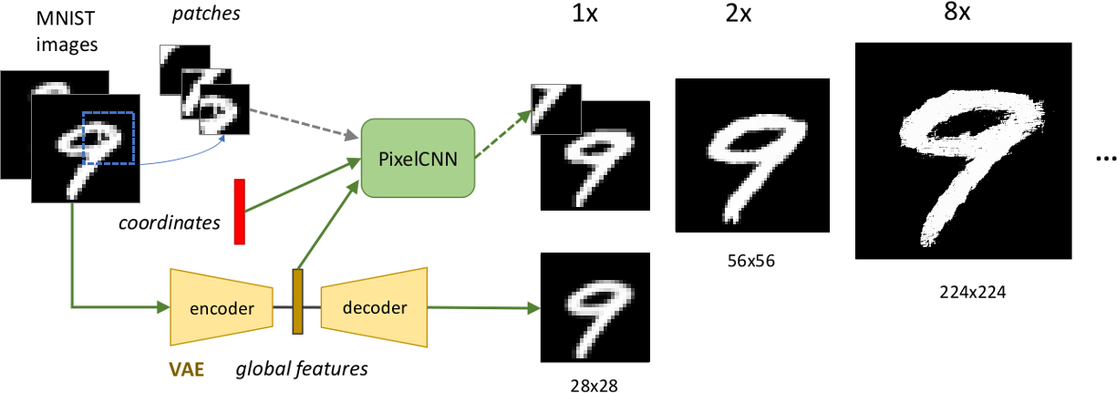
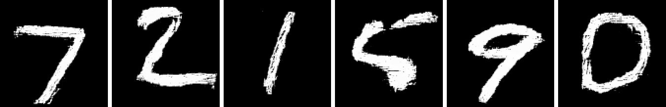
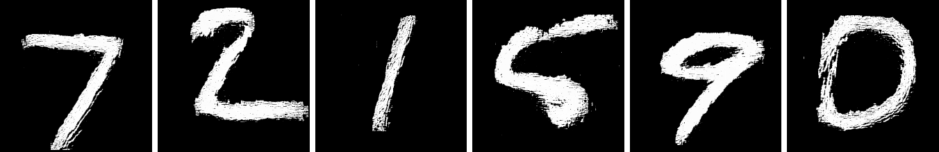
In this paper, we propose Spatial PixelCNN, a conditional autoregressive PixelCNN (Oord et al., 2016b) capable of generating large images from small patches. We combine the strengths of three components: (1) an autoregressive model—specifically, PixelCNN++ (Salimans et al., 2017)—to capture local image statistics from patches; (2) a latent variable model—in our case a variational autoencoder (Kingma & Welling, 2013)—to capture the global structures in images; and (3) spatial locations of each pixel in an image. Intuitively, an image is modeled autogressively pixel-by-pixel. Each pixel sampled is conditioned on (1) a subset of previously sampled pixels in its neighborhood; (2) a latent code that encodes global image statistics; and (3) 2-D spatial coordinates indicating its location in the image. This spatial conditioning enables us to reduce the coupling of each pixel from the resolution of the image. At generation time, our approach takes a target resolution as input, and outputs an image of arbitrary size (e.g. images from training patches, Fig. 2).
While performing impressively, state-of-the-art super-resolution techniques (Ledig et al., 2016; Tyka, 2017) (a) require a large dataset of high-resolution images—which may not be always available in practice; (b) have a fixed-sized output. We instead explore learning a generic upscaling function from only low-resolution images, in the absence of high-resolution images. Compared to existing image generative models that output fixed-sized images, our approach can be trained on small patches as opposed to full-sized images, thus requiring much less GPU memory—an important implication for scalability. Our method also enables the possibility of training on a dataset of images of mixed resolutions.
Our contributions are summarized as follows:
-
1.
We show the effects of spatial conditioning, using pixel coordinates, on generating high-resolution images.
- 2.
-
3.
We show that remarkably, Spatial PixelCNN is capable of generating coherent images at arbitrary resolutions for the MNIST dataset.
2 Related Work
Pixel Recurrent Neural Networks (Oord et al., 2016b) (PixelRNN), are a class of powerful generative model. PixelRNN is an explicit generative model which can be trained to directly maximize the likelihood of the training data. Here, the likelihood of each 2-D image is decomposed via chain rule into:
| (1) |
which is the product of every pixel , conditioned on all previous pixels in the row-major order—a left to right, top to bottom order of columns and rows .
It is this grounding in RNNs, that helps explain the motivation to train on only a patch of an image at time. RNNs have been used extensively for sequence modeling (Krause et al., 2016; Theis & Bethge, 2015; Kim et al., 2016). Often in the area of natural language processing (NLP), the corpus of text being trained is too large to feed the entire sequence of characters or words to the model at once. In order to circumvent that limitation, training involves a truncated form of backpropagation through time (Werbos, 1990; Graves, 2013). Our approach of training on patches can be seen as a similar trade-off. Rather than conditioning each pixel on all previous pixels in a given image, we only condition on a local window of pixels.
Pixel Convolutional Neural Networks (PixelCNN) (Oord et al., 2017), are a reformulation of PixelRNNs, that exploit masked convolutions to parallelize the the autoregressive computation. The approach of using masked convolutions for autoregressive density estimation has also been exploited for text (Kalchbrenner et al., 2016), audio (Oord et al., 2016a), and videos (Kalchbrenner et al., 2017).
Thus, there is reason to believe sequential modeling of pixels in an image can be achieved through training on patches utilizing a PixelCNN. Though to allow recreating the original image, there are several additional factors which are crucial to producing an adequate result.
2.1 Variational Autoencoders
Variational autoencoders (Kingma & Welling, 2013) are a form of latent variable model. They are trained to encode their input into a latent code . The true posterior is often intractable, so an approximate posterior is computed by optimizing a variational lower bound on the log-likelihood of the data. Often this latent code is interpretable and encodes a global representation of .
(Gulrajani et al., 2016; Chen et al., 2016) have evaluated integrating a PixelCNN decoder into a VAE framework. Gulrajani et al., 2016 note that it is critical to ensure the receptive field of the PixelCNN is smaller than the input image . Otherwise, a powerful PixelCNN decoder alone can model the entire image distribution, rendering the latent code from the VAE unused. When evaluated on binarized MNIST (Larochelle & Murray, 2011), both report the successful combination yields state-of-the-art results.
Spatial PixelCNN indeed fits the criteria needed to ensure utilization of the latent code , as it only trains on a patch of an image at a time. In fact the inclusion of a latent variable model, in this case a VAE, is necessary to ensure the model has a global representation of the images.
2.2 Conditioning on Pixel Coordinates
Compositional Pattern Producing Networks (CPPNs) (Stanley, 2007) are feedforward networks that utilize a wide array of transfer functions and are often trained via evolutionary algorithms. CPPNs can encode 2-D images (Nguyen et al., 2015), 3-D objects (Clune & Lipson, 2011) and even weights of another target network (Stanley et al., 2009).
To encode a 2-D color image, a CPPN performs a transformation parameterized by a network which takes as input a pair of coordinates and outputs 3 color values (e.g. RGB) (Secretan et al., 2008). A pair of coordinates is often computed by evenly sampling a pre-defined range e.g. . The coordinates are assembled into a grid, each corresponding to a pixel in the training image. At image generation time, an image can be rendered at an arbitrarily large resolution by simply sampling more coordinates within the specified range, and querying the CPPN for the associated color value.
CPPNs have been shown to impose a strong spatial prior yielding images of highly regular patterns (Secretan et al., 2008; Nguyen et al., 2015). It is this spatial regularity from CPPNs that we exploit in this work. We find that conditioning Spatial PixelCNN on a grid of coordinates is crucial for ensuring a coherent image is generated, and also confers an ability to upscale images.
2.3 Other High-Resolution Image Generation Methods
Since directly modeling high resolution images is challenging, an effective approach is to generate an image in hierarchical stages of increasing resolutions (Zhang et al., 2016; Denton et al., 2015; Karras et al., 2017). While producing impressive results, this approach outputs fixed-sized images, and requires storing the entire image in GPU memory at once—this is problematic when the training images exceed GPU memory capacity. Spatial PixelCNN instead allows for choosing the target image size at generation time, and only processes a small patch of the image at a time.
To cut down on GPU memory requirements, Tyka, 2017 devises upscaling image tiles, and stitching them together to produce the final result. While requiring less memory, the approach still retains the reliance on generating a fixed-sized output.
Our framework most closely resembles Ha, 2016, which combines spatial coordinates, and the latent code from a VAE, trained as a GAN end-to-end on full-sized images. Our model differs in two important ways: (1) Spatial PixelCNN conditions each pixel on the latent code and a local neighborhood of preceding pixels rather than assuming conditional independence given the latent code; (2) Spatial PixelCNN is trained on patches rather than full-sized images.
3 Methods
In this section we define the mathematical formulation of our model. We additionally describe how we generate images of a target size from the trained model.
3.1 Spatial PixelCNN
Our proposed model is based on a modified version of PixelCNN++ (Salimans et al., 2017). In order to reduce cumbersome mathematical notation, we restate Eq. 1 as:
| (2) |
where denotes the virtual index of the pixel, if the image were flattened into a 1-D array. Rather than training the model on full-sized images , we instead choose random patches of size taken from the images:
| (3) |
Given that our goal is to model the set of images , rather than merely a collection of all patches , we condition on a normalized coordinate grid that has the same number of coordinate pairs as pixels in the full-sized image. Specifically, is composed of evenly spaced coordinate pairs within the range . We choose patches from corresponding to the given patch . To condition each pixel on its corresponding coordinate pair , we make use of the gated spatial conditioning as outlined in van den Oord et al., 2016 arriving at the conditional probability:
| (4) |
We found such spatial conditioning crucial to imparting coherence to the patches . Without conditioning on , the model may assign a high probability to distinct patches of the generated image, allowing juxtapositions (Fig. 3). However, as the model is trained on patches of fewer dimensions, the extra spatial information provided by is not enough to ensure global coherence (Fig. 3(c)).
In order to provide this global coherence, we also condition on a latent code, provided by a VAE. Previous treatments (Gulrajani et al., 2016; Chen et al., 2016) combinining PixelCNN and VAE have made use of PixelCNN as a decoder. We found that by only training on patches, the VAE was unable to capture global features (data not shown). Instead, we jointly train the two models: VAE on images and Spatial PixelCNN on patches .
Specifically, we minimize the sum of an image loss and a patch loss:
| (5) |
The image loss is the typical VAE loss, that of the negative log-likelihood of the images and the KL-divergence of the approximate posterior from the prior:
| (6) |
The patch loss is the negative log-likelihood of the patches, given the coordinate grid and latent :
| (7) |
Note that instead of co-training both VAE and Spatial PixelCNN, it is also possible to pre-train the VAE first, and then train the Spatial PixelCNN. This pre-trained VAE typically has a lower KL-divergence than the co-trained approach. Global features extracted from the pre-trained VAE also allow for successful reconstructions, though we do not evaluate its efficacy in this paper.
3.2 Generating Images
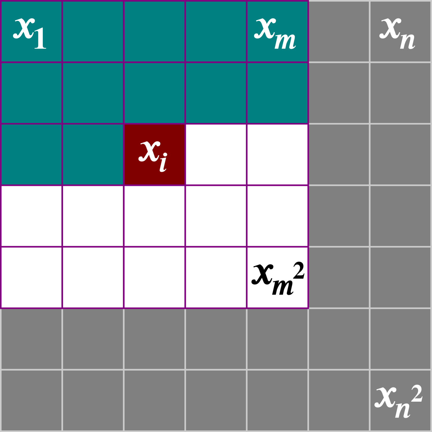
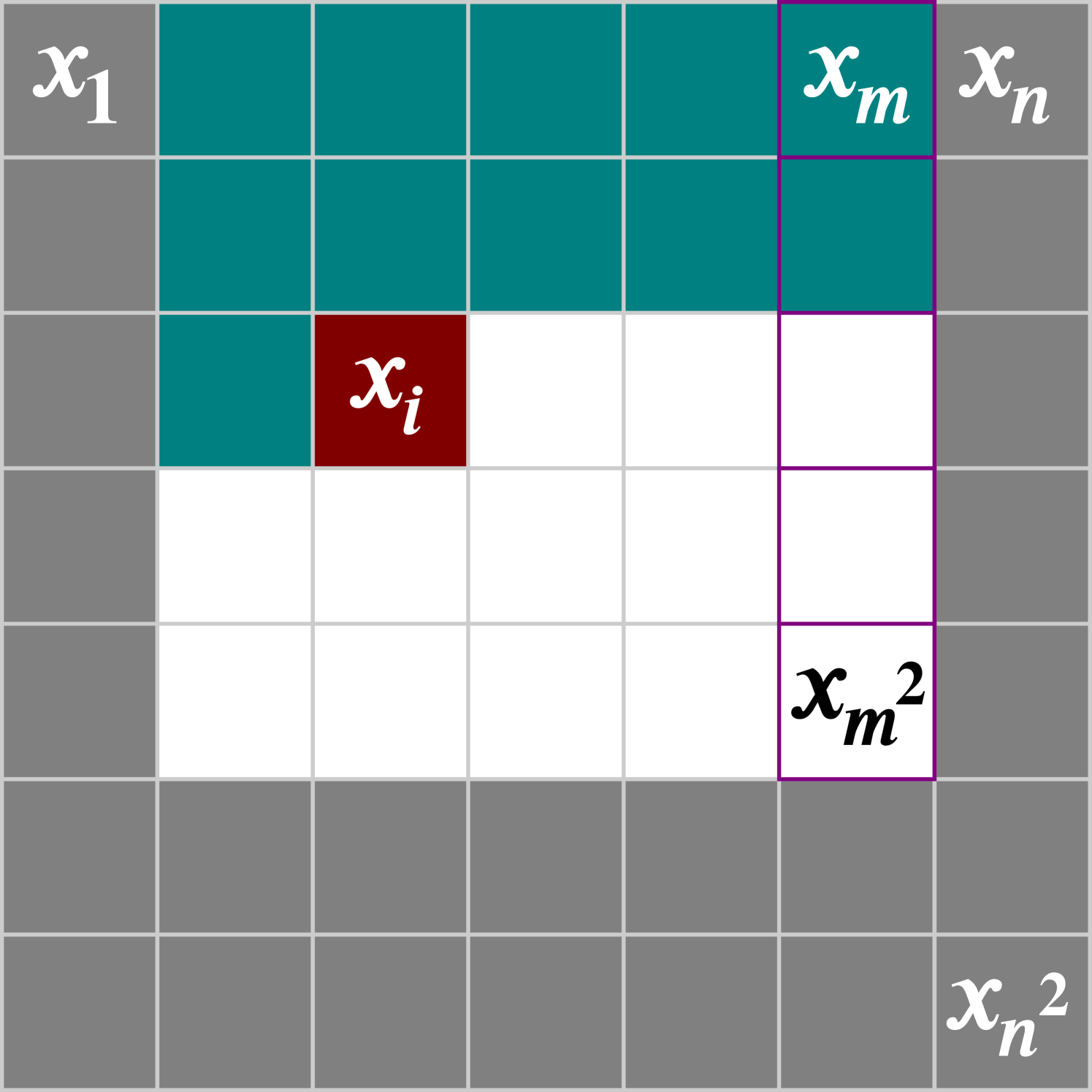
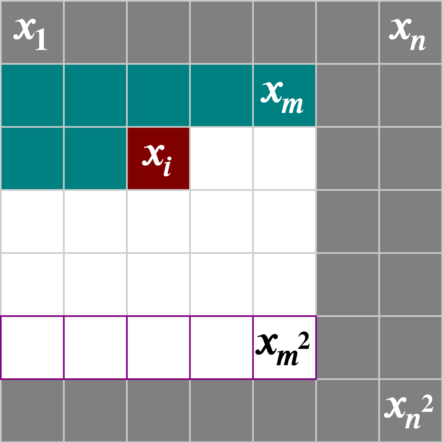
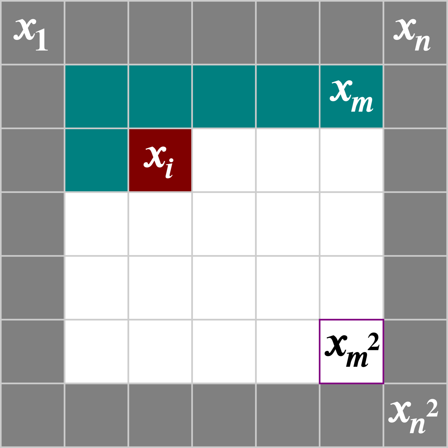
As our model is based on patches of images, a sliding window is used during image generation. In order to ensure that each pixel being generated has the maximal number of preceding pixels to condition on, the sliding window moves one pixel at a time from left to right, top to bottom (Fig. 4). This is the same ordering defined by the model for pixels to condition on (Eq. 1). Only the maximally conditioned pixels are generated from each patch of the sliding window.
One of the unique aspects of our model is its ability to upscale images to a higher resolution, while only being trained on lower resolution images. To accomplish this, we condition on coordinate patches from a larger coordinate grid during the generation process. That is, when we generate a image, we subdivide the grid into evenly spaced steps. Then as we slide the window over the image we wish to generate, we condition on the associated patch from .
4 Experiments
| PixelCNN++ without VAE | ||||||
| MS-SSIM | Confidence | |||||
| Patch Size | Coordinates | Bpd | 28x28 | 56x56 | 28x28 | 56x56 |
| * | 0.88 | 0.17 0.26 | 0.66 0.16 | 95.6 1.2 | 70.7 5.1 | |
| 0.89 | 0.17 0.27 | 0.48 0.29 | 97.5 0.7 | 86.3 3.3 | ||
| 1.50 | 0.09 0.25 | 0.15 0.19 | 89.6 2.6 | 82.1 3.6 | ||
| 1.48 | 0.18 0.26 | 0.27 0.15 | 93.7 1.7 | 81.5 3.5 | ||
| 1.68 | 0.03 0.24 | 0.02 0.12 | 87.0 2.9 | 79.9 3.7 | ||
| 1.65 | 0.14 0.25 | 0.15 0.18 | 91.1 2.3 | 82.6 3.7 | ||
| 1.73 | 0.02 0.24 | 0.02 0.13 | 86.4 3.0 | 80.3 3.8 | ||
| 1.70 | 0.13 0.24 | 0.20 0.19 | 85.6 3.5 | 83.3 3.5 | ||
| 1.52 | 0.05 0.21 | 0.05 0.14 | 71.8 6.0 | 76.3 4.3 | ||
| 1.42 | 0.14 0.23 | 0.17 0.19 | 79.1 5.5 | 86.4 2.9 | ||
| PixelCNN++ with VAE | ||||||
|---|---|---|---|---|---|---|
| MS-SSIM | Confidence | |||||
| Patch Size | Coordinates | Bpd | 28x28 | 56x56 | 28x28 | 56x56 |
| 1.95 | 0.03 0.23 | 0.03 0.11 | 87.6 2.8 | 81.9 3.5 | ||
| 1.87 | 0.19 0.27 | 0.16 0.21 | 93.4 1.6 | 91.3 2.3 | ||
| * | 1.39 | 0.18 0.27 | 0.15 0.21 | 97.0 0.8 | 93.2 1.7 | |
| 1.67 | 0.18 0.27 | 0.13 0.20 | 95.1 1.3 | 94.1 1.6 | ||
Here we describe the details for the experiments conducted. This includes model architecture, training hyperparameters, and the specific metrics used to evaluate the model.
4.1 Model Details
We use a modified version of PixelCNN++ (Salimans et al., 2017). Our model similarly makes use of six blocks of ResNet (He et al., 2016) layers. Spatial PixelCNN is conditioned on both a latent vector and a regularized coordinate grid. For each change in dimensions between blocks, the coordinate grid is resampled to the new layer’s dimensions. This resampling is performed as a simple linear interpolation. Given a grid patch defined by coordinates in the range , we linearly interpolate the range into equal sized steps. This regularization is key to preserving spatial coherence between ResNet blocks.
We additionally make use of ResNet blocks for the encoder and decoder of our VAE. For each ResNet layer of the decoder, we condition on the latent vector .
For most of our MNIST (LeCun et al., 1998) experiments we use two ResNet layers for each block, with a convolution filter size of . We term this the small network. In order to determine the trade-off between the model’s ability to compress data (as determined by having a smaller expected bits per dimension), versus its ability to effectively upscale images, we also conduct an experiment with a large network. This large network utilizes five ResNet layers for each block, with a convolution filter size of . The size of the latent code is fixed at for both network sizes.
4.2 Training Details
We make use of the Tensorflow (Abadi et al., 2015) framework for training and evaluating our models. We train using the Adam (Kingma & Ba, 2014) optimizer, with a batch size of , and an initial learning rate of of which is annealed using exponential decay at a rate of every batch. Additionally a dropout rate of , along with L2 regularization of is utilized. We train each model until convergence, as determined by a lack of improvement over one hundred epochs in the model’s bits per dimension.
At testing and image generation time we use the exponential moving average over the model parameters (Polyak & Juditsky, 1992), calculated with a decay of at each parameter update. We report our negative log-likelihood values in bits per dimension. The reported bits per dimension is calculated as the average bits per dimension over all possible patches for the images in the test set.
4.3 Evaluation Details
As previously noted (Theis et al., 2015), the negative log-likelihood may not be a great qualitative measure for evaluating generative models. This can be seen clearly in our experiments, where bits per dimension does not accurately correlate with the ability of the model to generate coherent images (Fig. 3).
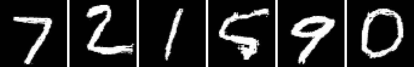
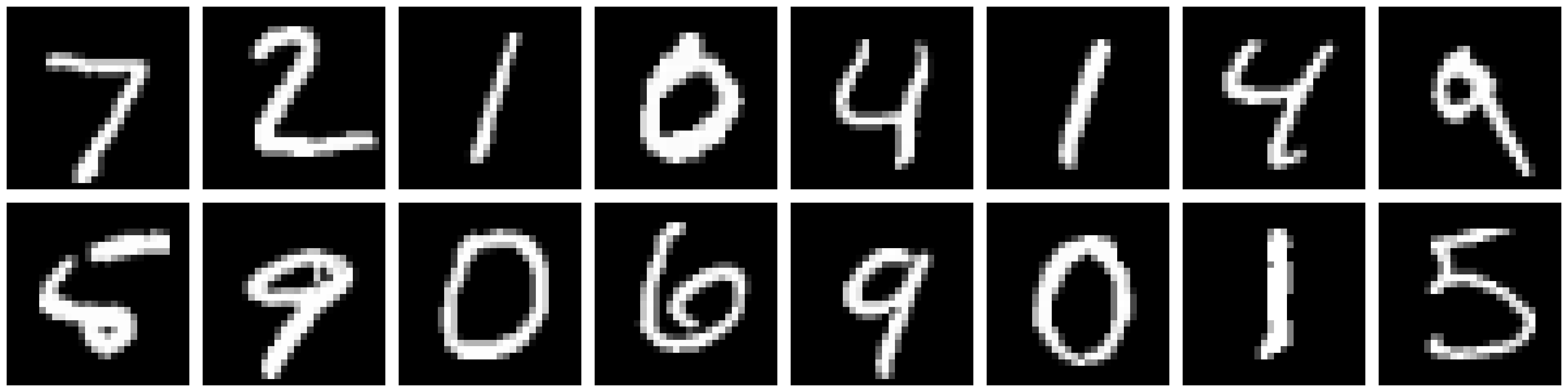
MS-SSIM: We first assess the diversity of the images generated by utilizing Multiscale Structural Similarity (Wang et al., 2003; Odena et al., 2016) (MS-SSIM). To calculate the MS-SSIM for a given model, we begin by randomly sampling images from the model. We produce an MS-SSIM score for all unique pairs of images. We then report the mean and standard deviation of these scores. The lower the MS-SSIM, the more diverse the images in the set. The ideal MS-SSIM of a given model should closely resemble that of the underlying data, so we also report an MS-SSIM for images from the MNIST test set for comparison.
While a measure of diversity shows the model does not exhibit mode collapse, it is unable to address the subjective assessment of image quality. Such an assessment should include the ability of the model to accurately reconstruct a given input, as well as ensuring generated samples reflect the underlying data distribution. Thus we devise two additional measures.
LeNet Accuracy: As the combination of PixelCNN and VAE allows for conditioning on an interpretable latent representation, we can assess reconstruction accuracy for these models. We take inspiration from the use of the Inception model (Odena et al., 2016) for assessing accuracy. As our model is trained on MNIST, we instead train a version of LeNet (LeCun et al., 1998), which has demonstrated strong classification ability for this dataset. We reconstruct images from the test set using our models, then measure the classification accuracy for these reconstructions. For comparison, we also report the classification accuracy for the original images from the test set.
LeNet Confidence: In order to assess random samples generated from the model, we devise a simple confidence score inspired by the Inception Score (Salimans et al., 2016). As part of the Inception Score measures diversity, we reformulate our metric to only measure the conditional probability of the label, given an image. For a given image, we calculate the softmax of the LeNet logits. The index of the largest value indicates the predicted class. We take the largest value multiplied by one hundred as a confidence measure, indicating how confident the model is in the prediction. We report the mean and standard deviation of this value for random samples from each model.
Given that our model additionally shows strong ability to upscale images to higher resolutions, we also report results for generating images. For both classification accuracy and confidence, we first downsample images to before running the LeNet classifier. We note that individually these metrics are imperfect, especially when assessing downsampled images, but when taken in aggregate they yield a more holistic assessment.
5 Results
| PixelCNN++ with VAE | |||
|---|---|---|---|
| Accuracy | |||
| Patch Size | Coordinates | 28x28 | 56x56 |
| 33.2 | 12.1 | ||
| 97.2 | 87.8 | ||
| * | 98.2 | 91.4 | |
| 96.2 | 95.3 | ||
In this section we detail the results of our experiments. As the model we propose has multiple components, we perform ablation experiments to verify the need for each. When comparing MS-SSIM scores, we consider scores close to those computed for the actual MNIST digits to be better scores. For LeNet Accuracy and Confidence, a higher score is considered better.
5.1 Effects of Spatial Conditioning
We first assess the importance of spatial conditioning on the generative ability of PixelCNN++ (Table 2). We train PixelCNN++ on various patch sizes, both with and without spatial conditioning. We note that even when trained on full-sized images, conditioning on a grid of coordinates boosts both MS-SSIM and LeNet Confidence (Table 2 Row 2). This implies the addition of coordinates may help capture structure versus a baseline PixelCNN++.
As we sweep across patch sizes, we see the addition of coordinates keeps the MS-SSIM within range of the underlying dataset. Though, we note as patch size decreases, we observe a decrease in confidence scores for the samples, and associated coherence of the resultant images (Fig. 3(c)).
An important observation from the experiments is that the trained bits per dimension value is not a great representation of the quality of random samples generated from the models (Figs. 3(b) & 3(c)). In the case of training on patches (Table 2 Row 2), the model achieves a similar ability to compress the data (as denoted by a low bits per dimension), as training on patches (Table 2 Row 2). Though, comparing the LeNet Confidence of generated images, the patches clearly model the underlying dataset more accurately (training on patches achieves a Confidence of , while training on patches only results in a score of ).
5.2 Addition of a Latent Code
We next consider the effects provided by the addition of a latent code. Even without spatial conditioning, the model trained on patches produces higher confidence scores with the addition of a VAE (Table 2 Row 2 & Table 2 Row 2). Though, the model has trouble with scale (Fig. 3(d)). This follows our intuition that spatial conditioning is key to capturing regularity across images.
5.3 Images from Patches
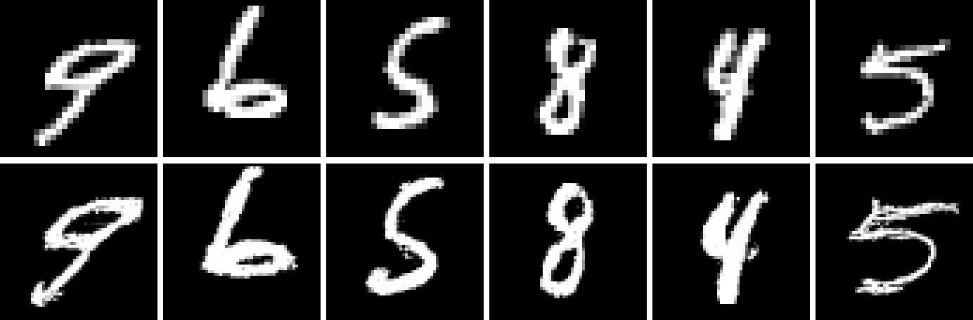
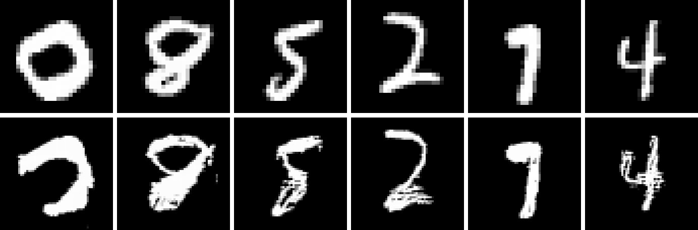
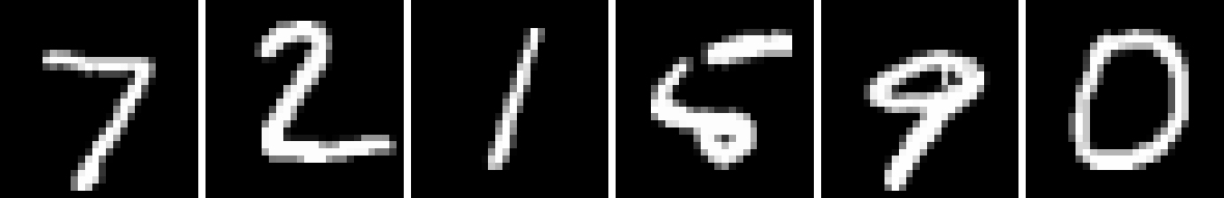
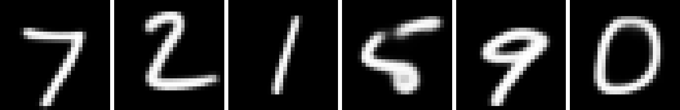
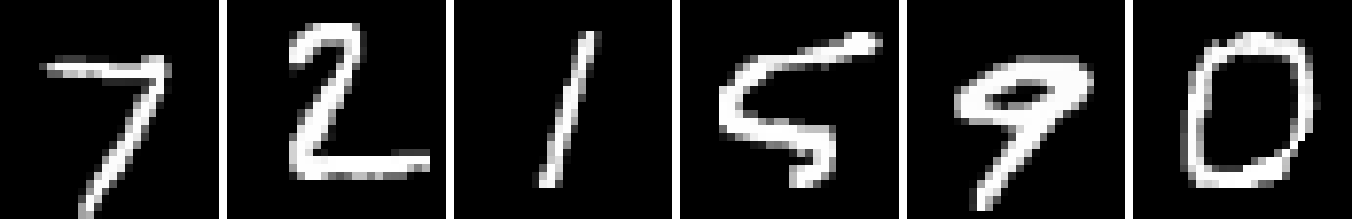
We now examine Spatial PixelCNN conditioned on both coordinates and a latent code. While a direct comparison is difficult, we note that Spatial PixelCNN produces samples qualitatively similar to PixelCNN++ (Fig. 1). Additionally Spatial PixelCNN trained on patches receives a similar Confidence score to the PixelCNN++ baseline when generating images (Table 2 Row 2 & Table 2 Row 2).
An interesting result can be observed when comparing the small network trained on patches versus the small network trained on patches. Given an equivalent network size, training on smaller patches produces superior results (Table 2 Rows 2 & 2). Only with the addition of more parameters, through the use of the large network, does training on patches produce a higher confidence and accuracy (Table 2 Rows 2 & 2) when generating images.
5.4 Upscaling Ability
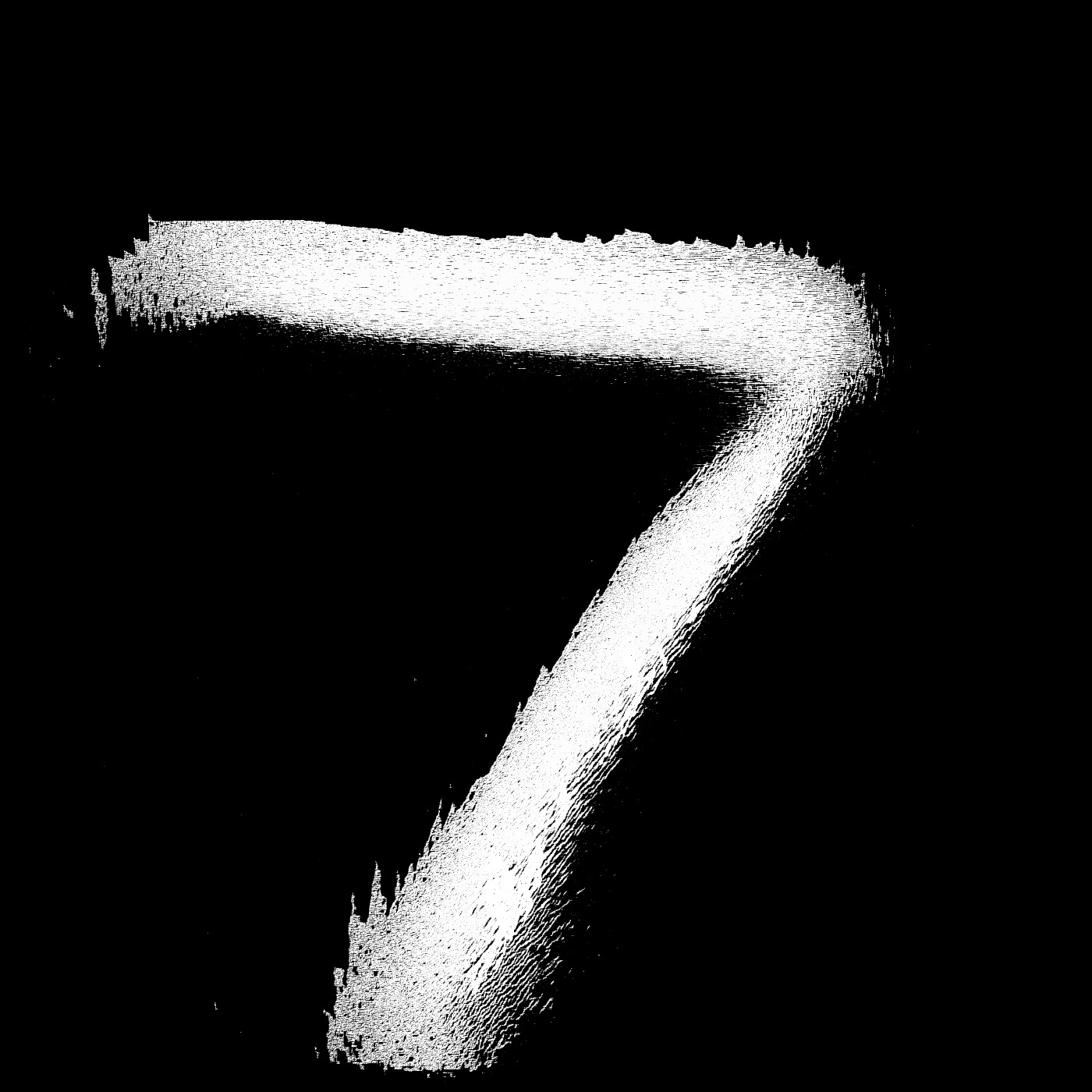
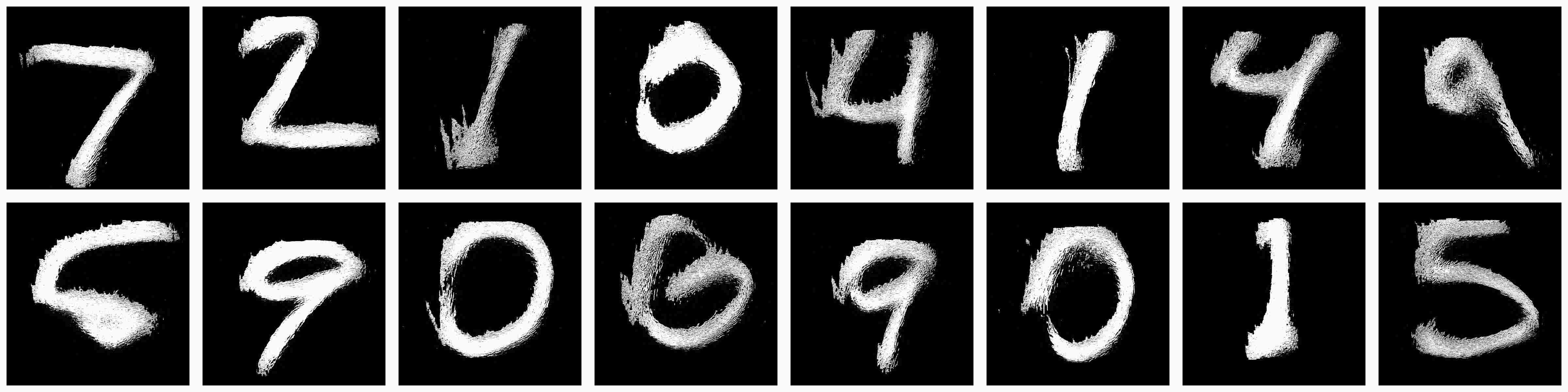
Finally we assess the ability for the network to generate high resolution images while only training on a low resolution dataset. Looking at the generated images, the small network trained on patches works exceedingly well for upscaling (Fig. 1(b)). It even tends to retain structural detail better than the large network trained on patches (Fig. 1(c)). Not only does it surpass the accuracy and confidence scores of the large network (Table 2 Rows 2 & 2 and Table 3 Rows 3 & 3), it only loses a small amount of accuracy and confidence, despite upscaling . It even shows remarkable ability for large upscaling factors (Figs. 2, 5(e), & 5(f)). See Appendix A for examples of and upscaling.
6 Discussion & Conclusions
We demonstrated that the addition of coordinates to PixelCNN++ has a clear positive effect on its generative ability. This can be seen even when trained on full-sized images, rather than on patches. We also showed that with the combination of a VAE, Spatial PixelCNN trained on patches is able to not only generate convincing images at the same resolution as the underlying dataset, but also high resolution images, despite only training on a low resolution dataset.
We believe that our approach should allow for training on mixed-sized images by feeding a resampled version of the image to the VAE. This may potentially allow for less preprocessing of images used for training. We leave this open for future research.
7 Acknowledgments
We thank Jeff Clune for his valuable discussions and support. We also thank the University of Wyoming Advanced Research Computing Center (ARCC) for their assistance and computing resources which enabled us to perform experiments and analyses. Additionally, we appreciate OpenAI making their code for PixelCNN++ available for reference online.
References
- Abadi et al. (2015) Abadi, Martín, Agarwal, Ashish, Barham, Paul, Brevdo, Eugene, Chen, Zhifeng, Citro, Craig, Corrado, Greg S., Davis, Andy, Dean, Jeffrey, Devin, Matthieu, Ghemawat, Sanjay, Goodfellow, Ian, Harp, Andrew, Irving, Geoffrey, Isard, Michael, Jia, Yangqing, Jozefowicz, Rafal, Kaiser, Lukasz, Kudlur, Manjunath, Levenberg, Josh, Mané, Dan, Monga, Rajat, Moore, Sherry, Murray, Derek, Olah, Chris, Schuster, Mike, Shlens, Jonathon, Steiner, Benoit, Sutskever, Ilya, Talwar, Kunal, Tucker, Paul, Vanhoucke, Vincent, Vasudevan, Vijay, Viégas, Fernanda, Vinyals, Oriol, Warden, Pete, Wattenberg, Martin, Wicke, Martin, Yu, Yuan, and Zheng, Xiaoqiang. TensorFlow: Large-scale machine learning on heterogeneous systems, 2015. URL https://www.tensorflow.org/. Software available from tensorflow.org.
- Arjovsky et al. (2017) Arjovsky, Martin, Chintala, Soumith, and Bottou, Léon. Wasserstein gan. 01 2017. URL https://arxiv.org/abs/1701.07875.
- Chen et al. (2016) Chen, Xi, Kingma, Diederik P, Salimans, Tim, Duan, Yan, Dhariwal, Prafulla, Schulman, John, Sutskever, Ilya, and Abbeel, Pieter. Variational lossy autoencoder. arXiv preprint arXiv:1611.02731, 2016.
- Clune & Lipson (2011) Clune, Jeff and Lipson, Hod. Evolving 3d objects with a generative encoding inspired by developmental biology. ACM SIGEVOlution, 5(4):2–12, 2011.
- Denton et al. (2015) Denton, Emily, Chintala, Soumith, Szlam, Arthur, and Fergus, Rob. Deep generative image models using a laplacian pyramid of adversarial networks. 06 2015. URL https://arxiv.org/abs/1506.05751.
- Goodfellow et al. (2014) Goodfellow, Ian, Pouget-Abadie, Jean, Mirza, Mehdi, Xu, Bing, Warde-Farley, David, Ozair, Sherjil, Courville, Aaron, and Bengio, Yoshua. Generative adversarial nets. In Advances in neural information processing systems, pp. 2672–2680, 2014.
- Graves (2013) Graves, Alex. Generating sequences with recurrent neural networks. arXiv preprint arXiv:1308.0850, 2013.
- Gulrajani et al. (2016) Gulrajani, Ishaan, Kumar, Kundan, Ahmed, Faruk, Taiga, Adrien Ali, Visin, Francesco, Vazquez, David, and Courville, Aaron. Pixelvae: A latent variable model for natural images. arXiv preprint arXiv:1611.05013, 2016.
- Ha (2016) Ha, David. Generating large images from latent vectors. http://blog.otoro.net/2016/04/01/generating-large-images-from-latent-vectors/, 2016.
- He et al. (2016) He, Kaiming, Zhang, Xiangyu, Ren, Shaoqing, and Sun, Jian. Deep residual learning for image recognition. In Proceedings of the IEEE conference on computer vision and pattern recognition, pp. 770–778, 2016.
- Kalchbrenner et al. (2016) Kalchbrenner, Nal, Espeholt, Lasse, Simonyan, Karen, Oord, Aaron van den, Graves, Alex, and Kavukcuoglu, Koray. Neural machine translation in linear time. arXiv preprint arXiv:1610.10099, 2016.
- Kalchbrenner et al. (2017) Kalchbrenner, Nal, van den Oord, Aäron, Simonyan, Karen, Danihelka, Ivo, Vinyals, Oriol, Graves, Alex, and Kavukcuoglu, Koray. Video pixel networks. In Precup, Doina and Teh, Yee Whye (eds.), Proceedings of the 34th International Conference on Machine Learning, volume 70 of Proceedings of Machine Learning Research, pp. 1771–1779, International Convention Centre, Sydney, Australia, 06–11 Aug 2017. PMLR. URL http://proceedings.mlr.press/v70/kalchbrenner17a.html.
- Karras et al. (2017) Karras, Tero, Aila, Timo, Laine, Samuli, and Lehtinen, Jaakko. Progressive growing of gans for improved quality, stability, and variation. arXiv preprint arXiv:1710.10196, 2017.
- Kim et al. (2016) Kim, Yoon, Jernite, Yacine, Sontag, David, and Rush, Alexander M. Character-aware neural language models. In AAAI, pp. 2741–2749, 2016.
- Kingma & Ba (2014) Kingma, Diederik and Ba, Jimmy. Adam: A method for stochastic optimization. arXiv preprint arXiv:1412.6980, 2014.
- Kingma & Welling (2013) Kingma, Diederik P and Welling, Max. Auto-encoding variational bayes. 12 2013. URL https://arxiv.org/abs/1312.6114.
- Krause et al. (2016) Krause, Ben, Lu, Liang, Murray, Iain, and Renals, Steve. Multiplicative lstm for sequence modelling. 09 2016. URL https://arxiv.org/abs/1609.07959.
- Larochelle & Murray (2011) Larochelle, Hugo and Murray, Iain. The neural autoregressive distribution estimator. In Proceedings of the Fourteenth International Conference on Artificial Intelligence and Statistics, pp. 29–37, 2011.
- LeCun et al. (1998) LeCun, Yann, Bottou, Léon, Bengio, Yoshua, and Haffner, Patrick. Gradient-based learning applied to document recognition. Proceedings of the IEEE, 86(11):2278–2324, 1998.
- Ledig et al. (2016) Ledig, Christian, Theis, Lucas, Huszár, Ferenc, Caballero, Jose, Cunningham, Andrew, Acosta, Alejandro, Aitken, Andrew, Tejani, Alykhan, Totz, Johannes, Wang, Zehan, et al. Photo-realistic single image super-resolution using a generative adversarial network. arXiv preprint arXiv:1609.04802, 2016.
- Nguyen et al. (2015) Nguyen, Anh, Yosinski, Jason, and Clune, Jeff. Deep neural networks are easily fooled: High confidence predictions for unrecognizable images. In Proceedings of the IEEE Conference on Computer Vision and Pattern Recognition, pp. 427–436, 2015.
- Nguyen et al. (2017) Nguyen, Anh, Yosinski, Jason, Bengio, Yoshua, Dosovitskiy, Alexey, and Clune, Jeff. Plug & play generative networks: Conditional iterative generation of images in latent space. Proceedings of the IEEE Conference on Computer Vision and Pattern Recognition, 2017.
- Nowozin et al. (2016) Nowozin, Sebastian, Cseke, Botond, and Tomioka, Ryota. f-gan: Training generative neural samplers using variational divergence minimization. In Advances in Neural Information Processing Systems, pp. 271–279, 2016.
- Odena et al. (2016) Odena, Augustus, Olah, Christopher, and Shlens, Jonathon. Conditional image synthesis with auxiliary classifier gans. arXiv preprint arXiv:1610.09585, 2016.
- Oord et al. (2016a) Oord, Aaron van den, Dieleman, Sander, Zen, Heiga, Simonyan, Karen, Vinyals, Oriol, Graves, Alex, Kalchbrenner, Nal, Senior, Andrew, and Kavukcuoglu, Koray. Wavenet: A generative model for raw audio. arXiv preprint arXiv:1609.03499, 2016a.
- Oord et al. (2016b) Oord, Aaron van den, Kalchbrenner, Nal, and Kavukcuoglu, Koray. Pixel recurrent neural networks. arXiv preprint arXiv:1601.06759, 2016b.
- Oord et al. (2017) Oord, Aaron van den, Vinyals, Oriol, and Kavukcuoglu, Koray. Neural discrete representation learning. arXiv preprint arXiv:1711.00937, 2017.
- Polyak & Juditsky (1992) Polyak, Boris T and Juditsky, Anatoli B. Acceleration of stochastic approximation by averaging. SIAM Journal on Control and Optimization, 30(4):838–855, 1992.
- Rezende et al. (2014) Rezende, Danilo Jimenez, Mohamed, Shakir, and Wierstra, Daan. Stochastic backpropagation and approximate inference in deep generative models. In Xing, Eric P. and Jebara, Tony (eds.), Proceedings of the 31st International Conference on Machine Learning, volume 32 of Proceedings of Machine Learning Research, pp. 1278–1286, Bejing, China, 22–24 Jun 2014. PMLR. URL http://proceedings.mlr.press/v32/rezende14.html.
- Salimans et al. (2016) Salimans, Tim, Goodfellow, Ian, Zaremba, Wojciech, Cheung, Vicki, Radford, Alec, and Chen, Xi. Improved techniques for training gans. In Advances in Neural Information Processing Systems, pp. 2234–2242, 2016.
- Salimans et al. (2017) Salimans, Tim, Karpathy, Andrej, Chen, Xi, and Kingma, Diederik P. Pixelcnn++: Improving the pixelcnn with discretized logistic mixture likelihood and other modifications. arXiv preprint arXiv:1701.05517, 2017.
- Secretan et al. (2008) Secretan, Jimmy, Beato, Nicholas, D Ambrosio, David B, Rodriguez, Adelein, Campbell, Adam, and Stanley, Kenneth O. Picbreeder: evolving pictures collaboratively online. In Proceedings of the SIGCHI Conference on Human Factors in Computing Systems, pp. 1759–1768. ACM, 2008.
- Stanley (2007) Stanley, Kenneth O. Compositional pattern producing networks: A novel abstraction of development. Genetic programming and evolvable machines, 8(2):131–162, 2007.
- Stanley et al. (2009) Stanley, Kenneth O, D’Ambrosio, David B, and Gauci, Jason. A hypercube-based encoding for evolving large-scale neural networks. Artificial life, 15(2):185–212, 2009.
- Theis & Bethge (2015) Theis, Lucas and Bethge, Matthias. Generative image modeling using spatial lstms. In Advances in Neural Information Processing Systems, pp. 1927–1935, 2015.
- Theis et al. (2015) Theis, Lucas, Oord, Aäron van den, and Bethge, Matthias. A note on the evaluation of generative models. arXiv preprint arXiv:1511.01844, 2015.
- Tyka (2017) Tyka, Mike. Superresolution with semantic guide. https://mtyka.github.io/machine/learning/2017/08/09/highres-gan-faces-followup.html, 2017.
- van den Oord et al. (2016) van den Oord, Aaron, Kalchbrenner, Nal, Espeholt, Lasse, Vinyals, Oriol, Graves, Alex, et al. Conditional image generation with pixelcnn decoders. In Advances in Neural Information Processing Systems, pp. 4790–4798, 2016.
- Wang et al. (2003) Wang, Zhou, Simoncelli, Eero P, and Bovik, Alan C. Multiscale structural similarity for image quality assessment. In Signals, Systems and Computers, 2004. Conference Record of the Thirty-Seventh Asilomar Conference on, volume 2, pp. 1398–1402. IEEE, 2003.
- Werbos (1990) Werbos, Paul J. Backpropagation through time: what it does and how to do it. Proceedings of the IEEE, 78(10):1550–1560, 1990.
- Zhang et al. (2016) Zhang, Han, Xu, Tao, Li, Hongsheng, Zhang, Shaoting, Huang, Xiaolei, Wang, Xiaogang, and Metaxas, Dimitris. Stackgan: Text to photo-realistic image synthesis with stacked generative adversarial networks. arXiv preprint arXiv:1612.03242, 2016.
Appendix A Large Upscaling Factors
A.1 Upscaling Comparisons
A.2 A Single High-Resolution Example