Spatio-temporal Gait Feature with Global Distance Alignment
Abstract
Gait recognition is an important recognition technology, because gait is not easy to camouflage and does not need cooperation to recognize subjects. However, many existing methods are inadequate in preserving both temporal information and fine-grained information, thus reducing its discrimination. This problem is more serious when the subjects with similar walking postures are identified. In this paper, we try to enhance the discrimination of spatio-temporal gait features from two aspects: effective extraction of spatio-temporal gait features and reasonable refinement of extracted features. Thus our method is proposed, it consists of Spatio-temporal Feature Extraction (SFE) and Global Distance Alignment (GDA). SFE uses Temporal Feature Fusion (TFF) and Fine-grained Feature Extraction (FFE) to effectively extract the spatio-temporal features from raw silhouettes. GDA uses a large number of unlabeled gait data in real life as a benchmark to refine the extracted spatio-temporal features. GDA can make the extracted features have low inter-class similarity and high intra-class similarity, thus enhancing their discrimination. Extensive experiments on mini-OUMVLP and CASIA-B have proved that we have a better result than some state-of-the-art methods.
Index Terms:
gait recognition, spatio-temporal feature extraction, distance alignment.I Introduction
Different from iris, fingerprint, face, and other biometric features, gait does not need the cooperation of subject in the process of recognition, and it can recognize the subject at a long distance in uncontrolled scenarios. Therefore, gait has broad applications in forensic identification, video surveillance, crime investigation, etc [1, 2]. As a visual identification task, its goal is to learn distinguishing features for different subjects. However, when learn spatio-temporal features from raw gait sequences, gait recognition is often disturbed by many external factors, such as various camera angles, different clothes/carrying conditions [3, 4, 5].
Many deep learning-based methods have been proposed to overcome these problems [6, 7, 8, 9, 10, 11]. DVGan uses GAN to produce the whole view space, which views angle from 0° to 180° with 1° interval to adapt the various camera angles [12]. GaitNet uses Auto-Encoder as their framework to learn the gait-related information from raw RGB images. It also uses LSTMs to learn the changes of temporal information to overcome the different clothes/carrying conditions [13]. GaitNDM encodes body shape and boundary curvature into a new feature descriptor to increase the robustness of gait representation [14]. GaitSet learns identity information from the set, which consists of independent frames, to adapt the various viewing angles and different clothes/carrying conditions [15]. Gaitpart employs partial features for human body description to enhance fine-grained learning [16]. One robust gait recognition method combines multiple types of sensors to enhance the richness of gait information [17]. Gii proposes a discriminant projection method based on list constraints to solve the perspective variance problem in cross-view gait recognition [18].
Previous methods have performed well in extracting temporal or spatial information, but still fall short in extracting spatio-temporal features at the same time. This problem is even worse when identifying subjects with similar walking postures. To solve this problem, we came up with a novel method: Spatio-temporal Gait Feature with Global Distance Alignment, which consists of Spatio-temporal Feature Extraction (SFE) and Global Distance Alignment (GDA). SFE includes Temporal Feature Fusion (TFF) and Fine-grained Feature Extraction(FFE). The proposed method enhances the discrimination of spatio-temporal gait features from two aspects: effective extraction of spatio-temporal gait features and reasonable refinement of extracted features. For effective extraction of spatio-temporal gait features, we first use TFF to fuse the most representative temporal features and then use FFE to extract fine-grained features from the most representative temporal features. After the above operations, spatio-temporal features of raw gait silhouettes can be fully extracted. For reasonable refinement of extracted features, we try to use the feature distribution of real-life unlabeled gait data as a benchmark to refine the extracted spatio-temporal gait features, this operation can further increase the intra-class similarity and inter-class dissimilarity of the extracted spatio-temporal gait features.
We will describe the advantages of the proposed method from the following three aspects:
-
•
We propose a concise and effective framework named Spatio-temporal Feature Extraction (SFE), which firstly uses TFF to fuse the most representative temporal features, and then uses FFE to extract fine-grained features from the most representative temporal features. SFE is also a lightweight network model that has fewer network parameters than GaitSet, GaitPart and other state-of-the-art methods.
-
•
We propose a Global Distance Alignment (GDA) technique, which uses the feature distribution of real-life unlabeled gait data as a benchmark to refine the extracted spatio-temporal gait features. GDA can greatly increase the intra-class similarity and inter-class dissimilarity of extracted spatio-temopral gait features, thus enhancing their discrimination.
-
•
Extensive experiments on CASIA-B and mini-OUMVLP have proved that our method have better performance than other state-of-the-art methods. It is worth noting that the proposed method achieves an average rank-1 accuracy of 97.0 on the CASIA-B gait dataset under NM conditions.
II Related Work
This section focuses on the work related to gait recognition. It first introduces the differences between appearance-based and model-based methods, and then mainly introduces the temporal feature extraction model and spatial feature extraction model in appearance-based methods.
Gait recognition. Current gait recognition methods can be categorized as model-based methods [19, 20, 21, 22, 23] and appearance-based methods [24, 25, 26, 27, 28]. Appearance-based methods use CNNs directly to learn the spatio-temporal features of the original gait sequences and then use feature matching to identify the gait sequence [29]. Model-based methods use a new representation to replace the original gait silhouettes as input. A representative model-based method is JointsGait [30], which uses the human joints of raw gait silhouettes to create gait graph structure and then extracts the spatio-temporal features from the gait graph structure by Graph Convolutional Network (GCN). However, when using this method to express the silhouettes in gait sequence, it often loses a lot of important detailed information and increases the difficulty of recognition. Other model-based methods also encounter this problem, so appearance-based methods have become the most mainstream gait recognition methods at present [7, 31, 32, 8, 33, 34, 35]. In this paper, the methods we mentioned later both belong to the appearance-based methods.
The efficiency of spatio-temporal feature extraction is an important factor to measure the quality of appearance-based methods[36], it will greatly affect the accuracy of recognition. Spatio-temporal feature extraction module can be divided into two parts: temporal feature extraction module[37] and spatial feature extraction module. 1) For the temporal feature extraction module, there have deep learning-based methods and traditional methods. The traditional methods first compress the original gait silhouettes into a single image and then use a convolutional neural network to extract the spatio-temporal features of that image [38, 39]. Although these traditional methods are simple, the following researchers have found that they do not preserve temporal information well and try to use deep learning-based methods to extract temporal features. LSTM [40, 41, 42] uses a repeated neural network module to preserve and extract the temporal information from raw gait sequences. GaitSet[15] observes that even if the gait sequences are shuffled, rearranging them into correct order is not difficult, and then uses shuffled silhouettes to learn spatio-temporal information to ensure the adaptability of various gait sequences. But both LSTM and GaitSet have some disadvantages: they have complex network structures and calculation processes. In this paper, we try to use several parallel convolution layers to extract global features from raw gait silhouettes and use a simple max operation to fuse the most representative temporal feature. This can simplify the network structure and use less calculation to effectively extract the temporal feature. It is worth noting that our method only uses 4 convolution layers and 2 pooling layers in total. 2) For the spatial feature extraction module, in [43], the idea of partial is introduced into gait recognition, and it is considered that different human parts will play different roles in the recognition of identity information. Therefore, the human body is divided into seven different components, and the influence of different parts on gait recognition is explored by removing the seven components in the average gait image and observing the change of recognition rate. It lays a foundation for the current use of the partial idea. GaitPart uses this idea in the field of deep learning to describe the human body to fully extract the fine-grained information, it divides multi-layer features into blocks to extract fine-grained features and achieves good results. However, GaitPart uses the idea of partial in shallow features and divides multi-layer features into blocks, which increases the complexity of the network. In this paper, we divide the high-level features only once to extract the fine-grained feature, and only a single convolution layer can get good performance. This interesting idea also greatly simplifies the network structure.
We fully consider the shortcomings of previous gait recognition methods in spatio-temporal feature extraction and propose our method: Spatio-temporal Gait Feature with Global Distance Alignment. It first designs a concise and effective spatio-temporal gait feature extraction (SFE) model to ensure the effective extraction of spatio-temporal gait features, and then uses the global distance alignment (GDA) technique to increase the intra-class similarity and inter-class dissimilarity of the extracted spatio-temporal gait features. Our method can effectively enhance the discrimination of gait sequence to ensure the accuracy of gait recognition.
III Our method
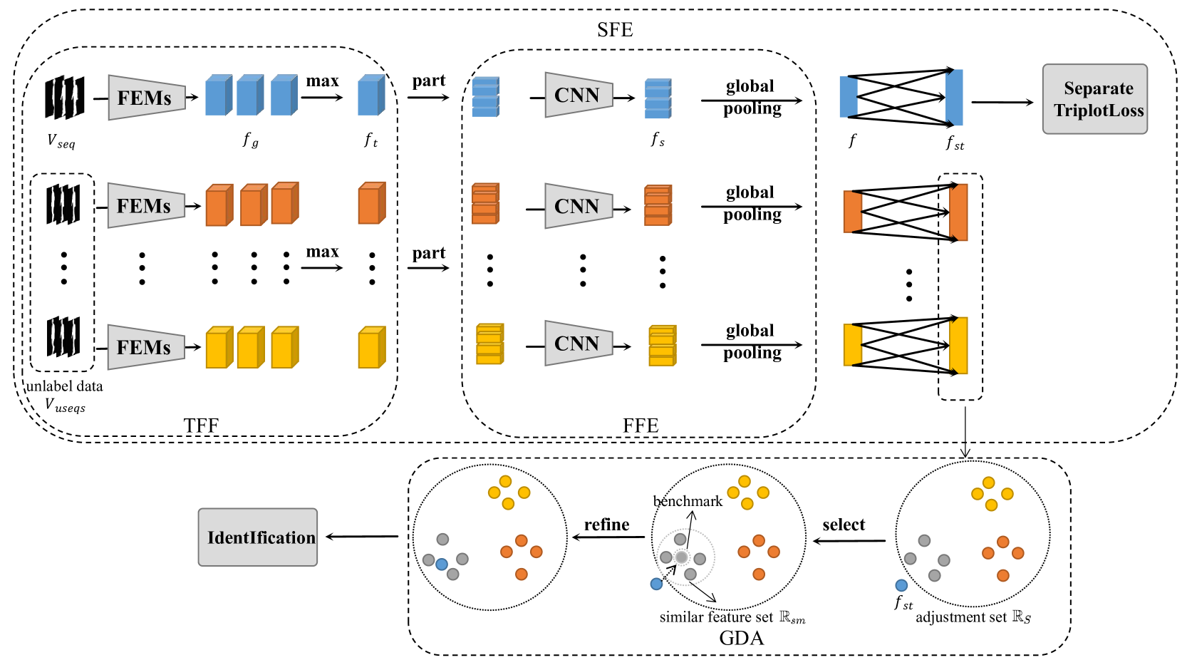
We will introduce our method from three aspects in this section, which includes the overall pipeline, Spatio-temporal Feature Extraction (SFE) module and Global Distance Alignment (GDA). SFE mainly includes two parts: Fine-grained Feature Extraction (FFE) and Temporal Feature Fusion (TFF). The framework of the proposed method is presented in Fig. 1.
III-A Pipeline
As presented in Fig. 1, our network mainly consists of two parts: SFE module and GDA module. SFE module is mainly the optimization of neural network structure, it can effectively extract the spatio-temporal gait features of raw gait sequences by a flexible network structure. GDA is a post-processing method, which uses a large number of unlabeled gait data in real life as a benchmark to refine the extracted spatio-temporal gait features. GDA can further enhance the discrimination of extracted gait features. It is worth noting that GDA is used in test phase, and it uses the trained SFE model as an extractor to extract the adjustment set.
At the part of SFE, we first input some raw gait silhouettes to TFF module frame by frame. TFF can learn the most representative temporal gait feature from the original gait sequence .
| (1) |
The most representative temporal gait feature are then sent to FFE module to learn their fine-grained feature .
| (2) |
After fine-grained features are extracted, a global pooling layer is used to remove redundant information of feature to obtain feature . Then the fully connected layer is used to integrate the spatio-temporal information of feature into . Finally, the Separate TripletLoss is used as a constraint to optimize network parameters.
At the part of GDA, we first use the trained SFE model to extract the spatio-temporal gait features of unlabel data as the adjustment set .
| (3) |
Then we select some similar spatio-temporal gait features from as similar feature set to refine the extracted feature to make it have high intra-class similarity and low inter-class similarity, thus enhancing its discrimination.
III-B Spatio-temporal Feature Extraction model
SFE model is mainly the optimization of neural network. It ensures that the spatio-temporal gait features are fully extracted while using as few network parameters as possible. We will introduce it from Temporal Feature Fusion (TFF) and Fine-grained Feature Extraction (FFE).
III-B1 Temporal Feature Fusion (TFF)
TFF consists of several parallel FEMs and a max pooling layer, where the parameters of FEMs are shared. FEMs are used to extract the global features from original gait sequence , they can fully extract the important information of each frame. Max pooling is used to select the most representative temporal feature from the global features . We will introduce the structure of FEM and why do we use Maxpooling to fuse the most representative temporal feature next.
| Feature Extraction Module | |||||
| Block | Layer | In | Out | Kernel | Pad |
| Block1 | Conv2d (C1) | 1 | 32 | 5 | 2 |
| Conv2d (C2) | 32 | 32 | 3 | 1 | |
| Maxpool, kernel size=2, stride=2 | |||||
| Block2 | Conv2d (C3) | 32 | 64 | 3 | 1 |
| Conv2d (C4) | 64 | 128 | 3 | 1 | |
| Maxpool, kernel size=2, stride=2 | |||||
As presented in Tab. I, FEM uses 4 Convolutional layers to extract the global features of raw silhouettes and 2 Max pooling layers to select the important information of these global features. These operations can fully extract the global features from original gait sequence.
| (4) |
We also find that only some features we extracted play an outstanding role in describing human identity. We try to use various operations: max, mean, medium to fuse the representative frame from extracted global features and then we find that using max operation can better preserve human identity information. The max operation is defined as:
| (5) |
where are the global features extracted from raw gait sequences by several parallel FEMs, is the most representative temporal feature fused from by max operation.
III-B2 Fine-grained Feature Extraction (FFE)
In the former literature, some researchers have found that using partial features to describe the human body has an outstanding performance. However, previous researches both analyze shallow partial features to describe the human body [44] and it needs to be partitioned many times in different layer features to extract fine-grained features, which will make the structure of the network more complex. So we try to extract the fine-grained features from deep layers to simplify network structure. It can ensure that we can fully extract fine-grained features while minimizing network parameters. We sequentially divide the extracted most representative temporal feature into 1, 2, 4, and 8 blocks to learn the fine-grained information, which the most representative temporal feature is a high-level feature. We can observe that when we use 4 blocks to learn the fine-grained features , it has the best performance. The results show that when we learn fine-grained information, excessive blocking can not make the fine-grained information learn more fully, but may ignore the relationship between adjacent parts. We also try to use deeper convolutional layers to learn fine-grained information again. But in most cases, its performance is not as good as the single Convolutional layer. The results strongly prove that when using the partial idea in high-level features, it does not need too deep network structure to learn fine-grained information.
Specifically, we first divide the most representative temporal feature into 4 blocks. Then use a single Convolutional layer to learn the fine-grained feature . After this, Global Pooling is used to reduce the redundant information of . The formula of Global Pooling is shown as:
| (6) |
These two pooling operations are both applied to the dimension. Through this operation, our feature changes from three-dimensional data containing , , and to two-dimensional data containing and . Finally, we use the Fully Connected Layer to integrate all the previously learned information to obtain the spatio-temporal gait feature .
Gait recognition is mainly based on feature matching to identify the identity of the subject. Therefore, the low similarity between different subjects and high similarity between the same subject are important factors to determine the recognition accuracy. The hard triplet loss has a good performance on reducing inter-class similarity and increasing intra-class similarity, so we use it as a constraint to optimize network parameters. Hard triplet loss is formulated as:
| (7) | ||||
where is a measure that represents the dissimilarity of the positive sample and anchor ( and ), is a measure that represents the dissimilarity of the negative sample and anchor ( and ). And we use the Euclidean norm to get the values of and . We use the min value of and the max value of as a proxy to calculate loss can be more effective in reducing inter-class similarity and increasing intra-class similarity.
III-C Global Distance Alignment
Triplet loss can increase intra-class similarity and decrease inter-class similarity of subjects in most cases. However, when meeting subjects with similar walking styles, triplet loss do not ensure the discrimination of their features. We try to use a post-processing method to refine the extracted spatio-temporal gait features to make them more discriminative. Global distance alignment technology is introduced to solve the problem. It pulls in the gait features between the same subjects to increase the intra-class similarity, and separates the gait features between different subjects to increase the inter-class dissimilarity.
First, we will find a large number of unlabeled gait data in real life. Then, we use the trained SFE module to extract spatio-temporal features of these unlabeled gait data. These extracted features are used as an adjustment set . And then, we calculate the distance between the features in and the extracted spatio-temporal features , and select some features similar to from based the calculated distance. These features are treated as similar feature sets . At the last, we adaptability select the most appropriate benchmark from by the overall (mean), maximum (maximum) and most moderate (median) aspects and use this benchmark to refine the extracted spatio-temporal features . Fig. 2 shows the complete feature refinement process. We can clearly see that after refinement by GDA, the intra-class similarity and inter-class dissimilarity of have greatly enhanced. Next, we will introduce GDA in detail from the following five parts: Unlabeled gait data, Adjustment set, Similar feature set, Benchmark and Refinement.
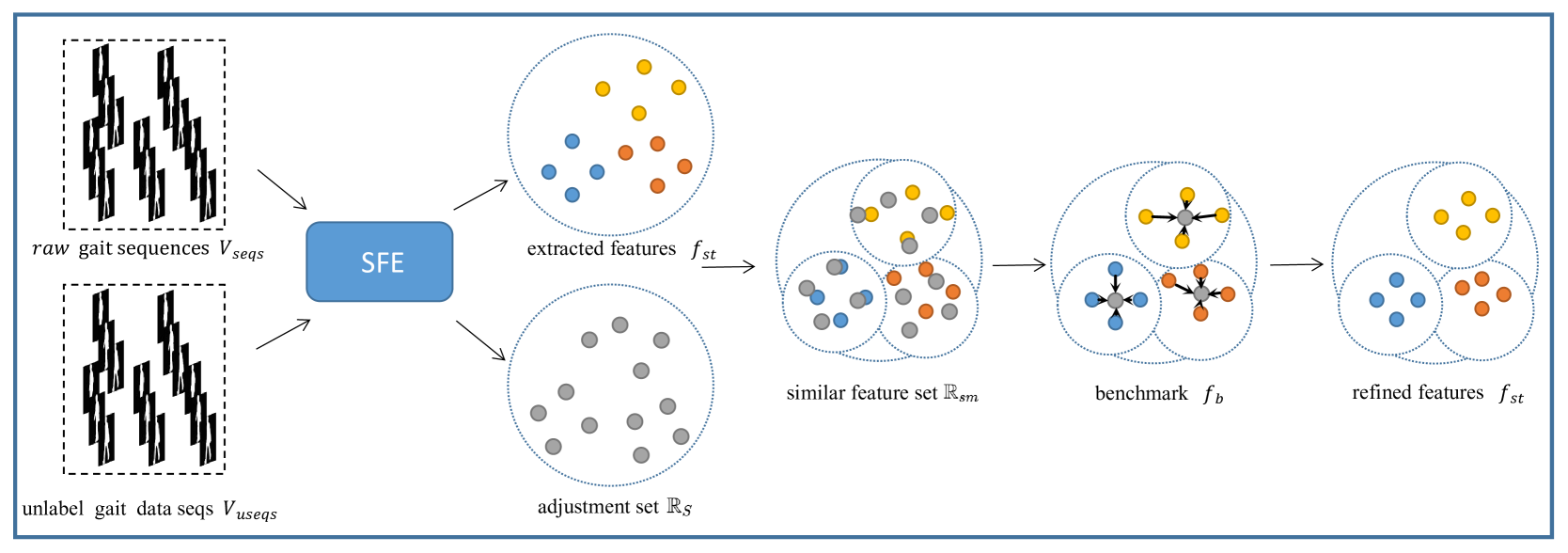
III-C1 Unlabeled gait data
The selection of unlabeled gait data directly determines the robustness of the adjustment set . It should be ensured that the unlabeled gait data should contain the appropriate number of subjects. If the number is small, it will not be representative enough, and if the number is large, it will lead to problems similar to overfitting. Fig. 3 of the experimental section verifies this conclusion. Another thing to note is that subjects in unlabeled gait data should have an appropriate sex ratio and a reasonable age distribution.
III-C2 Adjustment set
When unlabel gait data is found, we will use the trained SFE model to extract their spatio-temporal gait features and use these features as adjustment set . The formula for summarizing is defined as:
| (8) |
where are the gait sequences from the unlabeled gait data, which contains the appropriate number of subjects. is the adjustment set used to refine the spatio-temporal gait features .
III-C3 Similar feature set
When we get the adjustment set from unlabeled gait data , we first calculate the distance between these features in and extracted gait spatio-temporal features , and then select some features similar to from by the calculated distance. These features are treated as similar feature set . The formula for selecting the similar features is defined as:
| (9) | ||||
where is the spatio-temporal feature extracted from raw gait sequences in the probe set or gallery set, is the spatio-temporal feature in . is the spatio-temporal feature in . represents the distance between and . represents the distance between and . The distances mentioned here are measured by the Euclidean norm. This formula shows that the probability that the distance between and is smaller than the distance between and is . It can help us find some features , which most similar to extracted spatio-temporal features from .
III-C4 Benchmark
when we get , we will select the most appropriate benchmark to achieve the best refinement effect. The formula for determining is defined as:
| (10) | ||||
where has some features similar to the extracted saptio-temporal gait feature . , , respectively represent the maximum, average, and median values. can ensure that all similar features in are fully utilized, thus ensuring robustness of the benchmark . It is worth noting that for each extracted gait feature , the corresponding is different.
III-C5 Refinement
When the appropriate benchmark is calculated, we can use it to refine the previously extracted spatio-temporal gait features . This operation can make these features have hign intra-class similarity and inter-class dissimilarity, and make them more discriminative. The feature extracted in the test stage is divided into gallery set and probe set. When only the features in probe set are refined, the specific formula is defined as follows:
| (11) | ||||
where is the original distance between features in the probe set and features in the gallery set, it is an important reference to determine the identity of subject. is the value that spatio-temporal feature need to be refined, is the refined distance between in the probe set and in the gallery set. However, the formula only refines the features in probe set to modify the final distance for feature matching. When we want to refine the spatio-temporal gait features in both the gallery set and probe set, the formula can be defined as follows:
| (12) |
where is the value used to refine the spatio-temporal features in gallery set. and are hyperparameters that determine the degree of refinement. Extensive experiments have proved that GDA has the best effect when both and are set to 0.5.
| Gallery NM#1-4 | 0°-180° | mean | |||||||||||
|---|---|---|---|---|---|---|---|---|---|---|---|---|---|
| Probe | 0° | 18° | 36° | 54° | 72° | 90° | 108° | 126° | 144° | 162° | 180° | ||
| NM | CNN-LB [45] | 82.6 | 90.3 | 96.1 | 94.3 | 90.1 | 87.4 | 89.9 | 94.0 | 94.7 | 91.3 | 78.5 | 89.9 |
| GaitSet1 [15] | 90.8 | 97.9 | 99.4 | 96.9 | 93.6 | 91.7 | 95.0 | 97.8 | 98.9 | 96.8 | 85.8 | 95.0 | |
| Gait-Joint [13] | 75.6 | 91.3 | 91.2 | 92.9 | 92.5 | 91.0 | 91.8 | 93.8 | 92.9 | 94.1 | 81.9 | 89.9 | |
| GaitNet [9] | 91.2 | 92.0 | 90.5 | 95.6 | 86.9 | 92.6 | 93.5 | 96.0 | 90.9 | 88.8 | 89.0 | 91.6 | |
| CNN-Ensemble [45] | 88.7 | 95.1 | 98.2 | 96.4 | 94.1 | 91.5 | 93.9 | 97.5 | 98.4 | 95.8 | 85.6 | 94.1 | |
| GaitSet2 [46] | 91.1 | 99.0 | 99.9 | 97.8 | 95.1 | 94.5 | 96.1 | 98.3 | 99.2 | 98.1 | 88.0 | 96.1 | |
| GaitPart [16] | 94.1 | 98.6 | 99.3 | 98.5 | 94.0 | 92.3 | 95.9 | 98.4 | 99.2 | 97.8 | 90.4 | 96.2 | |
| Ours | 95.3 | 99.2 | 99.1 | 98.3 | 95.4 | 94.4 | 96.5 | 98.9 | 99.4 | 98.2 | 92.0 | 97.0 | |
| BG | CNN-LB [45] | 64.2 | 80.6 | 82.7 | 76.9 | 64.8 | 63.1 | 68.0 | 76.9 | 82.2 | 75.4 | 61.3 | 72.4 |
| GaitSet1 [15] | 83.8 | 91.2 | 91.8 | 88.8 | 83.3 | 81 | 84.1 | 90.0 | 92.2 | 94.4 | 79.0 | 87.2 | |
| GaitSet2 [46] | 86.7 | 94.2 | 95.7 | 93.4 | 88.9 | 85.5 | 89.0 | 91.7 | 94.5 | 95.9 | 83.3 | 90.8 | |
| MGAN [47] | 48.5 | 58.5 | 59.7 | 58.0 | 53.7 | 49.8 | 54.0 | 61.3 | 59.5 | 55.9 | 43.1 | 54.7 | |
| GaitNet [9] | 83.0 | 87.8 | 88.3 | 93.3 | 82.6 | 74.8 | 89.5 | 91.0 | 86.1 | 81.2 | 85.6 | 85.7 | |
| GaitPart [16] | 89.1 | 94.8 | 96.7 | 95.1 | 88.3 | 94.9 | 89.0 | 93.5 | 96.1 | 93.8 | 85.8 | 91.5 | |
| Ours | 91.3 | 94.9 | 95.5 | 93.64 | 90.5 | 84.4 | 90.8 | 95.8 | 97.6 | 94.14 | 88.0 | 92.4 | |
| CL | CNN-LB [45] | 37.7 | 57.2 | 66.6 | 61.1 | 55.2 | 54.6 | 55.2 | 59.1 | 58.9 | 48.8 | 39.4 | 54.0 |
| GaitSet1 [15] | 61.4 | 75.4 | 80.7 | 77.3 | 72.1 | 70.1 | 71.5 | 73.5 | 73.5 | 68.4 | 50.0 | 70.4 | |
| GaitSet2 [46] | 59.5 | 75.0 | 78.3 | 74.6 | 71.4 | 71.3 | 70.8 | 74.1 | 74.6 | 69.4 | 54.1 | 70.3 | |
| MGAN [47] | 23.1 | 34.5 | 36.3 | 33.3 | 32.9 | 32.7 | 34.2 | 37.6 | 33.7 | 26.7 | 21.0 | 31.5 | |
| GaitNet [9] | 42.1 | 58.2 | 65.1 | 70.7 | 68.0 | 70.6 | 65.3 | 69.4 | 51.5 | 50.1 | 36.6 | 58.9 | |
| Ours | 73.0 | 86.4 | 85.6 | 82.7 | 76.8 | 74.3 | 77.1 | 80.7 | 79.6 | 77.6 | 64.7 | 78.0 | |
| probe | Gallery All 14 Views | |
|---|---|---|
| GaitPart(experiment) | Ours | |
| 0° | 73.5 | 77.0 |
| 15° | 79.4 | 84.0 |
| 30° | 87.2 | 88.5 |
| 45° | 87.1 | 88.4 |
| 60° | 83.0 | 85.6 |
| 75° | 84.2 | 87.3 |
| 90° | 81.5 | 85.7 |
| 180° | 73.6 | 78.4 |
| 195° | 79.8 | 84.7 |
| 210° | 87.3 | 88.0 |
| 225° | 88.3 | 89.3 |
| 240° | 83.8 | 86.2 |
| 255° | 84.1 | 86.1 |
| 270° | 82.0 | 86.3 |
| mean | 82.5 | 85.4 |
IV Experiments
There are four parts to our experiment: the first part is an introduction of CASIA-B, mini-OUMVLP and training details. The second part shows the results of our method compared with other state-of-the-art methods. The third part is the ablation experiment, which describes the effectiveness of each module of the proposed method. The last part is an additional experiment, which presents the application of the proposed method on the cross dataset.
IV-A Datasets and Training Details
CASIA-B [48] is the main database to test the effectiveness of the gait method. It has a total of sequences, which 124 mean the number of subjects, 10 mean the groups of each subject, 11 mean angles of each group. Its walking conditions include walking in coats (CL), walking with a bag (BG) and normal walking (NM). CL has 2 groups, BG has 2 groups, NM has 6 groups. 11 angles include 0°, 18°, 36° 54°, 72°, 90°, 108°, 126°, 144°, 162°, 180°. The first 74 subjects of CASIA-B are used as the training set and the last 50 subjects are considered as the test set. The test set is divided into gallery set and probe set. The first 4 sequences in NM condition is set to gallery set, and the rest sequences are divided into 3 probe sets: BG #1-2, CL #1-2, NM #5-6.
mini-OUMVLP [49] evolved from OU-MVLP [50]. The number of original OU-MVLP is too large and the requirement of GPU is high, so we choose the first 500 subjects of OU-MVLP as our dataset: mini-OUMVLP. Each subject of mini-OUMVLP has 2 groups (#00-01), each group has 14 views (0°, 15°, …, 90°; 180°, 195°, …, 270°). The first 350 subjects of mini-OUMVLP are used as the training set, the rest 150 subjects are used as the test set. Seq #01 in the test set is set to gallery set and Seq #00 in the test set is set to probe set.
In all experiments, we crop the size of input silhouettes to 64 × 44 and consider 50 gait silhouettes as a gait sequence. We use adam as the optimizer for the model. The margin of hard triplet loss is set to 0.2.
1) In the dataset CASIA-B, we train the proposed method 78K iterations. GaitSet has been trained on 80K iterations. GaitPart has been trained on 120k iterations. The parameter settings of GaitPart and GaitSet are followed as their original papers. The parameters and are set to 8 and 16 respectively. The number of channels in both 1 and 2 is set as 32, 3 is set as 64, 4 is set as 128. The block for FFE is set as 4. The learning rate of this module is set as 1-4. We simulate real-life unlabeled gait data with gait sequences from the test set and extract the adjustment set by the proposed Spatio-temporal Feature Extraction module. The probability for selecting similar features is set to 0.001.
2) In the dataset mini-OUMVLP, we train the proposed method 120K iterations. GaitPart has been trained on 120k iterations. The parameter settings of GaitPart are followed as its original paper. The number of channels in both 1 and 2 is set as 32, 3 is set as 64, is set as 128. The number of blocks for FFE is set as 4. The parameters and are set to 8 and 16 respectively. The learning rate of this module is also set as 1-4. We also simulate real-life unlabeled gait data with gait sequences from the test set and extract the adjustment set by the proposed Spatio-temporal Feature Extraction module. The probability for selecting similar features is set to 0.001.
3) In additional experiments, we train proposed method 120k iterations on CASIA-B. The batch size is set to 8 16. The numbers of channels for both 1 and 2 is set as 32, 3 is set as 64, 4 is set as 128. The block for FFE is set as 4. The learning rate of this module is also set as 1-4. We test the proposed method on mini-OUMVLP. The first 350 subjects in mini-OUMVLP are simulated as unlabeled gait data in real life, and the next 150 subjects are used as the test set. The probability for selecting similar features is set to 0.001.
| probe | Fine-Grained Feature Extraction (FFE) | Feature alignment | walking conditions | |||||||||
| 8blocks | 4blocks | 2blocks | 1blocks | 4blocks+8blocks | 4blocks+4blocks | 0.001 | 0.01 | 0.1 | NM | BG | CL | |
| a | ✓ | 94.5 | 86.8 | 75.4 | ||||||||
| b | ✓ | 95.5 | 90.1 | 74.4 | ||||||||
| c | ✓ | 95 | 87.4 | 70.6 | ||||||||
| d | ✓ | 95 | 86.4 | 70.2 | ||||||||
| e | ✓ | 94.7 | 85.6 | 71.9 | ||||||||
| f | ✓ | 95.0 | 84.6 | 64.4 | ||||||||
| g | ✓ | ✓ | 97.0 | 92.4 | 78.0 | |||||||
| h | ✓ | ✓ | 96.1 | 91.5 | 76.3 | |||||||
| i | ✓ | ✓ | 96 | 90.8 | 75.6 | |||||||
IV-B Results
We have done a lot of experiments on CASIA-B and mini-OUMVLP, and the results proved that the proposed method has better performance than some state-of-the-art methods.
CASIA-B. Tab. II shows the results of some experiments with our method and some state-of-the-art methods. Except for our method, we also use GaitSet and GaitPart to do experiments on CASIA-B and the results of other methods are directly taken from their original papers. On normal walking conditions (NM), our accuracy at all views is greater than 90, and the average accuracy can achieve 97.0, even better than Gaitpart. On walking with a bag (BG), the average accuracy can achieve 92.4, and only two views (90°, 180°) are below 90. On walking in coats (CL), the average accuracy can achieve 78.0, and we are the best on all views compared with other state-of-the-art works.
mini-OUMVLP. In order to verify the robustness of our method, we try to do some experiments on another larger data set: mini-OUMVLP. Tab. III shows the results of our experiments. Because the original OU-MVLP dataset has so many subjects that it requires a lot of CPU resources, we use a smaller version that contained only the first 500 subjects of OU-MVLP. We keep the parameter settings of GaitPart as their original experiment. It should be notice that the original data of mini-OUMVLP are incomplete , so the identification accuracy will be a little affected. The average accuracy of all views of our method is 85.4, even better than GaitPart, which accuracy is 82.5. We are proud to have a higher performance than GaitPart in all 14 views.
| probe | Gallery All 14 Views | |
|---|---|---|
| Ours(Adjustment) | Ours(No Adjustment) | |
| 0° | 74.3 | 70.8 |
| 15° | 81.6 | 79.9 |
| 30° | 87.1 | 87.3 |
| 45° | 87.0 | 87.1 |
| 60° | 83.2 | 82.5 |
| 75° | 85.0 | 83.8 |
| 90° | 83.0 | 82.3 |
| 180° | 76.4 | 73.6 |
| 195° | 81.8 | 80.6 |
| 210° | 86.1 | 85.9 |
| 225° | 86.2 | 86.8 |
| 240° | 84.0 | 83.2 |
| 255° | 83.0 | 82.4 |
| 270° | 83.0 | 81.8 |
| mean | 83.0 | 82.0 |
IV-C Ablation Experiments
To prove the role of every part of the proposed method. We perform several ablation experiments on CASIA-B with different parameters, including setting different numbers of the blocks in Fine-grained Feature Extraction (FFE) and the different probability in Global Distance Alignment (GDA). The results are shown as Tab. IV. We will analyze these results in the next part.
Effectiveness of FFE. In order to explore how fine-grained features can be adequately extracted. We do different experiments on the number of blocks of FFE. 8 blocks, 4 blocks, 2 blocks, and 1 block mean that we divide the most representative temporal feature into 8 parts, 4 parts, 2 parts, and 1 part to extract the fine-grained spatial feature. 4 blocks + 8 blocks means that we divide the most representative temporal feature into 4 parts for fine-grained feature extractions, and then divide it into 8 parts again for further extraction of the fine-grained feature. 4 blocks + 4 blocks means that we divide the most representative temporal feature into 4 parts to learn the fine-grained features and then divide it into 4 parts again to further extract fine-grained features. 1) By comparing the groups a, b, c, d, we find that when we divide the most representative temporal features into 4 parts to extract the fine-grained features, it shows the best performance. This can prove that when we use the partial idea to extract fine-grained features, it is necessary to block the feature map to appropriate parts. If the most representative temporal feature is divided too fine, the information will be repeatedly extracted, and if the feature graph is divided too coarse, the fine-grained information will not be fully extracted. Both of them will affect the accuracy of recognition. 2) By comparing groups b, e, and f, we can observe that when we divide the most representative temporal feature into 4 parts and extract fine-grained features only once can get the best result. This can prove that the most representative temporal features extracted by Temporal Feature Fusion (TFF) are high-level features, so it only needs to block once and then extract fine-grained features once can fully obtain fine-grained features, and too much extraction will lead to information loss, which has a great impact on recognition accuracy. The results of the experiments can also show the advantages of our Spatio-temporal Feature Extraction module: spatial features can be fully extracted by using only one blocking operation in high-level features, which simplifies the structure of the network.
Effectiveness of GDA. GDA is not to optimize the network structure, it belongs to the post-processing of data, it uses unlabeled data set as the benchmark to refine the spatio-temporal features in the probe set and gallery set to make them have low inter-class similarity and high intra-class similarity. We will prove its effectiveness through some experiments. The most important part of GDA is to select the appropriate benchmark from the adjustment set to refine spatio-temporal features in gallery set and probe set. The most important factor to select an appropriate benchmark is to find some features similar to spatio-temporal features from . We will experiment to find out how many similar features we should find to have the best performance. 0.1, 0.01, 0.001 are the important similarity indicator to find similar feature set . These mean that the probability that the distance between in and is smaller than the distance between in and are 0.1, 0.01, 0.001 respectively. 1) By comparing the groups g, h, and i, it can be clearly observed that when we set the probability to 0.001, the result will be best. This can prove that only a small part of the data in is related to the spatio-temporal features , So we can not set the possibility too high. 2) By comparing the groups b and g, we can see the significance of GDA, the accuracies on NM, BG, and CL both get a good promotion after being refined by GDA. This fully proves that when we use GDA to refine the spatio-temporal features can make them have low inter-class similarity and high intra-class similarity, thus increasing their discrimination.
IV-D Additional Experiments
The training phase and test phase are all under the same data set on previous experiments, and the unlabeled data used for GDA is the test set. To further prove the robustness of the GDA module, we try to experiment on cross dataset. We first train the proposed Spatio-temporal Feature Extraction (SFE) module on CAISA-B, when the network parameters are trained, we do the test on mini-OUMVLP. We use the gait sequences of the first 350 subjects of mini-OUMVLP as the unlabeled gait sequences , and then use the trained SFM module to extract their spatio-temporal gait features as the adjustment set . Finally, we use the rest 150 subjects as the test set to test the effectiveness of GDA. Tab. V presents our results on mini-OUMVLP. Adjustment means that we refine the extracted spatio-temporal gait features in the probe set and gallery set by GDA before the test, and No means test without the refinement by GDA. It can be seen that after the processing of GDA, the recognition accuracies can be effectively improved. This cross dataset experiment can further prove the robustness of GDA.
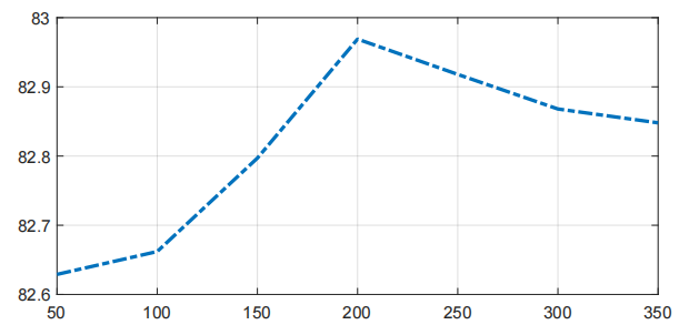
We also do some experiments to explore how many subjects should be used as the unlabeled data set. Fig. 3 shows how the final recognition accuracy varies with the number of subjects who are used to as the unlabeled gait data. We can observe that at the beginning, with the increase of the number of subjects, the accuracy of recognition becomes higher and higher. But as the number of subjects reaches a threshold, if we continue to increase the number of subjects, the recognition accuracy will decrease. This shows that we should choose the appropriate number of subjects when we find the unlabeled gait data, too few subjects may lead to the unlabeled data lacking representativeness, and too many subjects may lead to problems like overfitting.
V Conclusion
In this paper, we propose an interesting idea of using global distance alignment techniques to enhance the discrimination of features. Thus our method is proposed. It first uses Fine-grained Feature Extraction (FFE) and Temporal Feature Fusion (TFF) to effectively learn the spatio-temporal features from raw gait silhouettes, then uses a large number of unlabeled gait data in real life as a benchmark to refine the extracted spatio-temporal features to make them have low inter-class similarity and high intra-class similarity, thus enhancing their discrimination. Extensive experiments have proved that our method has a great performance on two main gait datasets: mini-OUMVLP and CASIA-B. In the future, we will try to introduce hyperspectral data sets and radar data sets to extract robust features for the task of gait recognition.
References
- [1] M. J. Marín-Jiménez, F. M. Castro, R. Delgado-Escaño, V. Kalogeiton, and N. Guil, “Ugaitnet: Multimodal gait recognition with missing input modalities,” IEEE Transactions on Information Forensics and Security, vol. 16, no. 1, pp. 5452–5462, 2021.
- [2] S. Choi, J. Kim, W. Kim, and C. Kim, “Skeleton-based gait recognition via robust frame-level matching,” IEEE Transactions on Information Forensics and Security, vol. 14, no. 10, pp. 2577–2592, 2019.
- [3] Y. He, J. Zhang, H. Shan, and L. Wang, “Multi-task gans for view-specific feature learning in gait recognition,” IEEE Transactions on Information Forensics and Security, vol. 14, no. 1, pp. 102–113, 2018.
- [4] X. Li, M. Chen, F. Nie, and Q. Wang, “A multiview-based parameter free framework for group detection.” in Proc. AAAI Conference on Artificial Intelligence, 2017, pp. 4147–4153.
- [5] X. Li, L. Liu, and X. Lu, “Person reidentification based on elastic projections,” IEEE Transactions on Neural Networks and Learning Systems, vol. 29, no. 4, pp. 1314–1327, 2018.
- [6] J. Su, Y. Zhao, and X. Li, “Deep metric learning based on center-ranked loss for gait recognition,” in Proc. IEEE International Conference on Acoustics, Speech and Signal Processing, 2020, pp. 4077–4081.
- [7] J. Liao, A. Kot, T. Guha, and V. Sanchez, “Attention selective network for face synthesis and pose-invariant face recognition,” in Proc. IEEE International Conference on Image Processing, 2020, pp. 748–752.
- [8] X. Ma, N. Sang, X. Wang, and S. Xiao, “Deep regression forest with soft-attention for head pose estimation,” in Proc. IEEE International Conference on Image Processing, 2020, pp. 2840–2844.
- [9] Z. Zhang, L. Tran, X. Yin, Y. Atoum, X. Liu, J. Wan, and N. Wang, “Gait recognition via disentangled representation learning,” in Proc. IEEE Conference on Computer Vision and Pattern Recognition, 2019, pp. 4710–4719.
- [10] Z. Zhang, L. Tran, X. Yin, Y. Atoum, X. Liu, J. Wan, and N. Wang, “Gait recognition via disentangled representation learning,” in Proc. IEEE Conference on Computer Vision and Pattern Recognition, 2019, pp. 4705–4714.
- [11] F. M. Castro, M. J. Marin-Jimenez, N. Guil, and N. P. de la Blanca, “Multimodal feature fusion for cnn-based gait recognition: an empirical comparison,” Neural Computing and Applications, vol. 32, no. 17, pp. 14 173–14 193, 2020.
- [12] R. Liao, W. An, S. Yu, Z. Li, and Y. Huang, “Dense-view geis set: View space covering for gait recognition based on dense-view gan.” arXiv preprint arXiv:2009.12516, 2020.
- [13] C. Song, Y. Huang, Y. Huang, N. Jia, and L. Wang, “Gaitnet: An end-to-end network for gait based human identification,” Pattern Recognition, vol. 96, no. 1, p. 106988, 2019.
- [14] H. El-Alfy, I. Mitsugami, and Y. Yagi, “Gait recognition based on normal distance maps,” IEEE transactions on cybernetics, vol. 48, no. 5, pp. 1526–1539, 2017.
- [15] H. Chao, Y. He, J. Zhang, and J. Feng, “Gaitset: Regarding gait as a set for cross-view gait recognition,” vol. 33, no. 1, pp. 8126–8133, 2019.
- [16] C. Fan, Y. Peng, C. Cao, X. Liu, S. Hou, J. Chi, Y. Huang, Q. Li, and Z. He, “Gaitpart: Temporal part-based model for gait recognition,” in Proc. IEEE Conference on Computer Vision and Pattern Recognition, 2020, pp. 14 225–14 233.
- [17] Q. Zou, L. Ni, Q. Wang, Q. Li, and S. Wang, “Robust gait recognition by integrating inertial and rgbd sensors,” IEEE transactions on cybernetics, vol. 48, no. 4, pp. 1136–1150, 2017.
- [18] Z. Zhang, J. Chen, Q. Wu, and L. Shao, “Gii representation-based cross-view gait recognition by discriminative projection with list-wise constraints,” IEEE transactions on cybernetics, vol. 48, no. 10, pp. 2935–2947, 2017.
- [19] W. An, S. Yu, Y. Makihara, X. Wu, C. Xu, Y. Yu, R. Liao, and Y. Yagi, “Performance evaluation of model-based gait on multi-view very large population database with pose sequences,” IEEE Transactions on Biometrics, Behavior, and Identity Science, vol. 2, no. 4, pp. 421–430, 2020.
- [20] R. Liao, S. Yu, W. An, and Y. Huang, “A model-based gait recognition method with body pose and human prior knowledge,” Pattern Recognition, vol. 98, no. 1, p. 107069, 2020.
- [21] S. Yan, Y. Xiong, and D. Lin, “Spatial temporal graph convolutional networks for skeleton-based action recognition,” in Proc. AAAI conference on artificial intelligence, 2018, pp. 1–1.
- [22] D. Kastaniotis, I. Theodorakopoulos, and S. Fotopoulos, “Pose-based gait recognition with local gradient descriptors and hierarchically aggregated residuals,” Journal of Electronic Imaging, vol. 25, no. 6, p. 063019, 2016.
- [23] J. Chen, J. Chen, H. Chao, and M. Yang, “Image blind denoising with generative adversarial network based noise modeling,” in Proc. IEEE Conference on Computer Vision and Pattern Recognition, 2018, pp. 3155–3164.
- [24] S. Yu and R. Liao, “Weizhi an, haifeng chen, edel b. garcía, yongzhen huang, and norman poh. gaitganv2: Invariant gait feature extraction using generative adversarial networks,” Pattern Recognition, vol. 87, no. 1, pp. 179–189, 2019.
- [25] Y. Wang, B. Du, Y. Shen, K. Wu, G. Zhao, J. Sun, and H. Wen, “Ev-gait: Event-based robust gait recognition using dynamic vision sensors,” in Proc. of the IEEE Conference on Computer Vision and Pattern Recognition, 2019, pp. 6358–6367.
- [26] I. Rida, “Towards human body-part learning for model-free gait recognition,” arXiv preprint arXiv:1904.01620, 2019.
- [27] G. Ma, L. Wu, and Y. Wang, “A general subspace ensemble learning framework via totally-corrective boosting and tensor-based and local patch-based extensions for gait recognition,” Pattern Recognition, vol. 66, no. 1, pp. 280–294, 2017.
- [28] M. Gadaleta and M. Rossi, “Idnet: Smartphone-based gait recognition with convolutional neural networks,” Pattern Recognition, vol. 74, no. 1, pp. 25–37, 2018.
- [29] X. Ben, P. Zhang, Z. Lai, R. Yan, X. Zhai, and W. Meng, “A general tensor representation framework for cross-view gait recognition,” Pattern Recognition, vol. 90, no. 1, pp. 87–98, 2019.
- [30] N. Li, X. Zhao, and C. Ma, “Jointsgait: A model-based gait recognition method based on gait graph convolutional networks and joints relationship pyramid mapping,” arXiv preprint arXiv:2005.08625, 2020.
- [31] A. Sepas-Moghaddam, S. Ghorbani, N. F. Troje, and A. Etemad, “Gait recognition using multi-scale partial representation transformation with capsules.” arXiv preprint arXiv:2010.09084, 2020.
- [32] B. Lin, S. Zhang, X. Yu, Z. Chu, and H. Zhang, “Learning effective representations from global and local features for cross-view gait recognition.” arXiv preprint arXiv:2011.01461, 2020.
- [33] C. Zhao, X. Li, and Y. Dong, “Learning blur invariant binary descriptor for face recognition,” Neurocomputing, vol. 404, no. 1, pp. 34–40, 2020.
- [34] Z. Ji, X. Liu, Y. Pang, and X. Li, “Sgap-net: Semantic-guided attentive prototypes network for few-shot human-object interaction recognition,” Proc. AAAI Conference on Artificial Intelligence, pp. 11 085–11 092, 2020.
- [35] Y. Fu, Y. Wei, Y. Zhou, H. Shi, G. Huang, X. Wang, Z. Yao, and T. Huang, “Horizontal pyramid matching for person re-identification,” in Proc. AAAI conference on artificial intelligence, 2019, pp. 8295–8302.
- [36] M. Deng, C. Wang, F. Cheng, and W. Zeng, “Fusion of spatial-temporal and kinematic features for gait recognition with deterministic learning,” Pattern Recognition, vol. 67, no. 1, pp. 186–200, 2017.
- [37] C. Wang, J. Zhang, J. Pu, X. Yuan, and L. Wang, “Chrono-gait image: A novel temporal template for gait recognition,” in Proc. European Conference on Computer Vision, 2010, pp. 257–270.
- [38] J. Han and B. Bhanu, “Individual recognition using gait energy image,” IEEE Transactions on Pattern Analysis and Machine Intelligence, vol. 28, no. 2, pp. 316–322, 2005.
- [39] K. Shiraga, Y. Makihara, D. Muramatsu, T. Echigo, and Y. Yagi, “Geinet: View-invariant gait recognition using a convolutional neural network,” in Proc International Conference on Biometrics, 2016, pp. 1–8.
- [40] G. Zhang, V. Davoodnia, A. Sepas-Moghaddam, Y. Zhang, and A. Etemad, “Classification of hand movements from eeg using a deep attention-based lstm network,” IEEE Sensors Journal, vol. 20, no. 6, pp. 3113–3122, 2019.
- [41] Y. Feng, Y. Li, and J. Luo, “Learning effective gait features using lstm,” in Proc. International Conference on Pattern Recognition, 2016, pp. 325–330.
- [42] A. Sepas-Moghaddam, A. Etemad, F. Pereira, and P. L. Correia, “Facial emotion recognition using light field images with deep attention-based bidirectional lstm,” in Proc. IEEE International Conference on Acoustics, Speech and Signal Processing, 2020, pp. 3367–3371.
- [43] X. Li, S. J. Maybank, S. Yan, D. Tao, and D. Xu, “Gait components and their application to gender recognition,” IEEE Transactions on Systems, Man, and Cybernetics, Part C (Applications and Reviews), vol. 38, no. 2, pp. 145–155, 2008.
- [44] T. T. Verlekar, L. D. Soares, and P. L. Correia, “Gait recognition in the wild using shadow silhouettes,” Image and Vision Computing, vol. 76, no. 1, pp. 1–13, 2018.
- [45] Z. Wu, Y. Huang, L. Wang, X. Wang, and T. Tan, “A comprehensive study on cross-view gait based human identification with deep cnns,” IEEE Transactions on Pattern Analysis and Machine Intelligence, vol. 39, no. 2, pp. 209–226, 2017.
- [46] H. Chao, K. Wang, Y. He, J. Zhang, and J. Feng, “Gaitset: Cross-view gait recognition through utilizing gait as a deep set,” IEEE Transactions on Pattern Analysis and Machine Intelligence, vol. 44, no. 7, pp. 3467–3478, 2021.
- [47] Y. He, J. Zhang, H. Shan, and L. Wang, “Multi-task gans for view-specific feature learning in gait recognition,” IEEE Transactions on Information Forensics and Security, vol. 14, no. 1, pp. 102–113, 2019.
- [48] S. Zheng, J. Zhang, K. Huang, R. He, and T. Tan, “Robust view transformation model for gait recognition,” in proc. IEEE International Conference on Image Processing, 2011, pp. 2073–2076.
- [49] Y. Chen, Y. Zhao, and X. Li, “Effective gait feature extraction using temporal fusion and spatial partial,” in Proc. IEEE International Conference on Image Processing, 2021, pp. 1244–1248.
- [50] N. Takemura, Y. Makihara, D. Muramatsu, T. Echigo, and Y. Yagi, “Multi-view large population gait dataset and its performance evaluation for cross-view gait recognition,” IEEE Transactions on Computer Vision and Applications, vol. 10, no. 1, pp. 1–14, 2018.