Spatio-Temporal Sparsification for General Robust Graph Convolution Networks
Abstract
Graph Neural Networks (GNNs) have attracted increasing attention due to its successful applications on various graph-structure data. However, recent studies have shown that adversarial attacks are threatening the functionality of GNNs. Although numerous works have been proposed to defend adversarial attacks from various perspectives, most of them can be robust against the attacks only on specific scenarios. To address this shortage of robust generalization, we propose to defend the adversarial attacks on GNN through applying the Spatio-Temporal sparsification (called ST-Sparse) on the GNN hidden node representation. ST-Sparse is similar to the Dropout regularization in spirit. Through intensive experiment evaluation with GCN as the target GNN model, we identify the benefits of ST-Sparse as follows: (1) ST-Sparse shows the defense performance improvement in most cases, as it can effectively increase the robust accuracy by up to 6% improvement; (2) ST-Sparse illustrates its robust generalization capability by integrating with the existing defense methods, similar to the integration of Dropout into various deep learning models as a standard regularization technique; (3) ST-Sparse also shows its ordinary generalization capability on clean datasets, in that ST-SparseGCN (the integration of ST-Sparse and the original GCN) even outperform the original GCN, while the other three representative defense methods are inferior to the original GCN.
1 Introduction
Recently, Graph Neural Networks (GNNs) have attracted increasing attention due to its successful applications on various graph-structure data, such as social networks, chemical composition structures, and biological gene proteins (Zhou et al. 2018; Wu et al. 2019b). However, recent works (Sun et al. 2018; Xu et al. 2019a; Dai et al. 2018) have pointed out that GNNs are vulnerable to adversarial attacks, which can crash safety-critical GNN applications, such as auto-driving, medical diagnosis (Wu et al. 2019b).
To address this issue, numerous works (Sun et al. 2018; Zhang, Cui, and Zhu 2020; Jin et al. 2020) have been proposed to defend the adversarial attacks from the perspectives of data preprocessing (Wu et al. 2019a), structure modification (Wang et al. 2019), adversarial training (Feng et al. 2019), adversarial detection (Zhang, Hossain Khan, and Coates 2019), and etc. However, our experimental study and the evaluation in the existing work (Jin et al. 2020) have shown that none of the existing defense methods is superior to the others under all attacks for all datasets with all perturbation sizes. This illustrates the limitation of the existing defense methods in terms of the robust generalization capability.
Recently, (Tsipras et al. 2019) revealed that the existence of adversarial attack might originate from the utilization of weakly correlated features, which can be reduced by keeping only the strongly correlated features. This phenomenon motivates us to adopt the sparse representation, which is widely utilized in computational neuroscience (Ahmad and Scheinkman 2019), to reduce the effect from the weakly correlated features. Thus, in this work, we propose a spatio-temporal feature sparsification framework to improve the robustness of the GNN models.
The spatial feature sparsification (called TopK) in the proposed framework simply keeps the features with the largest values and sets all the other features to zero. In spirit, TopK is the same as the Dropout regulirazation technique (Srivastava et al. 2014) except that Dropout randomly drops neurons, while TopK orders the neurons according to their output values and keeps only the neurons with the top values. Through experiment studies, we identify that TopK can improve the defense performance under four representative adversarial attacks on three typical benchmark datasets with varies perturbation sizes.
However, the robustness brought by TopK is at the expense of the generalization capability. Compared with Dropout, TopK loses the randomness, which sacrifices the generalization capability, as the randomness in Dropout can decompose a complex model into an ensemble of a large number of simpler models. To address this issue, temporal feature sparsification is introduced to alternate the non-zero features (also called active features) in each training epoch. Through the feature alternation, more features can participate in node representation in turn. Thus, the spatial sparsification together with the temporal sparsification (abbreviated as ST-Sparse) can behave similarly to the Dropout regulirazation technique. Therefore, ST-Sparse might achieve the similar generalization capability as Dropout. Moreover, through experiment evaluation, we identify that ST-Sparse can achieve robust generalization in that it can integrate with the existing defense methods to further improve the model robustness, similar to the integration of Dropout into various deep learning models as a standard regularization technique.
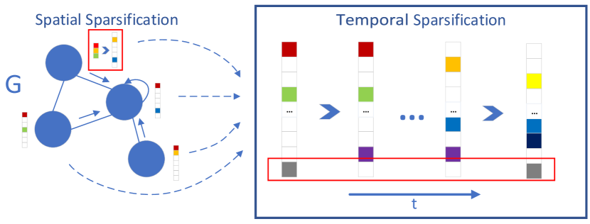
Fig. 1 illustrates the basic idea of the proposed ST-Sparse mechanism. The spatial sparsification is mainly dedicated to transform a dense hidden node vector of a GNN to a sparse high-dimensional vector, where only the top salient features are activated, as illustrated through the red rectangle at the top left part of Fig. 1. The temporal sparsification further sparsifies the active features along the time dimension during the GNN training process. More specifically, the duty cycle of each active feature dimension is sparse so that each active feature will not be intensively used.
Note that the temporal sparsification is applied to the feature dimension instead of the features of individual nodes, because on one hand, the salient features of individual nodes usually focus only on a few dimensions, the temporal spasification of these features may significantly degrade the model performance; on the other hand, the overall distribution composed of all nodes can better reflect the temporal sparsity. By balancing the duty cycle of activation among different dimension, it is possible to avoid the intensive usage of certain dimensions, thereby increasing the model’s expressive capability, which in turn increases the robustness of the model.
The main contributions of this work is summarized as follows.
-
•
From the perspective of spatio-temporal sparsity, we explore to construct a robust feature space, where the information propagation in GNN is less vulnerable to adversarial attacks.
-
•
We provide a novel ST-Sparse mechanism, which utilizes TopK to realize spatial sparsity in high-dimensional vector space, and adopts attention to balance the activation duty cycles among different dimensions, so as to realize the temporal sparsity in the feature space.
-
•
To verify the effectiveness of ST-Sparse, we apply ST-Sparse to the graph convolution network (GCN) (Kipf and Welling 2017) (denoted as ST-SparseGCN). Intensive experiments through three benchmark datasets show that ST-SparseGCN can significantly improve the robustness, robust generalization, and ordinary generalization of GCN in terms of classification accuracy.
2 Related Works
Adversarial attacks on general graph. The basic idea of adversarial attacks on graph is to change the graph topology or feature information to intentionally interfere with the classifier. (Dai et al. 2018) studied a non-target evasion attack based on reinforcement learning. (Zügner, Akbarnejad, and Günnemann 2018) proposed netattack, a poisoning attack on GCN, which modifies the training data to misclassify the target node. Further, (Zügner and Günnemann 2019) used the meta-gradient to solve the min-max problem in attacks during training, and proposed an attack method that reduces the overall classification performance. Besides, (Xu et al. 2019b) simplified the discrete graph problem by convex relaxation, and thus proposed a gradient-based topological attack.
Defense methods on general graph. The existing defense methods can be classified from the perspectives of data preprocessing (Wu et al. 2019a), structure modification (Wang et al. 2019), adversarial training (Feng et al. 2019), the modificaiton of the objective function (Bojchevski and Günnemann 2019), adversarial detection (Zhang, Hossain Khan, and Coates 2019), and hybrid defense (Chen et al. 2019). The proposed ST-SparseGCN model can be regarded as a structure modification methods, because it modifies the original GCN structure, as shown in Fig. 2. However, the proposed ST-Sparse defense methods can also be integrated with the other GCN defense models, such as GCN-Jaccard(Wu et al. 2019a) and GCN-SVD(Entezari et al. 2020), which can be regarded as data preprocessing methods. Thus, the integrated models can be classified as hybrid defense models. Although dozens of defense methods on graph have been proposed, none of them shows the robust generalization, as they are not superior to the others under all attacks for all datasets with all perturbation sizes (Jin et al. 2020).
Sparsity and Robustness. The relation between sparsity and robustness has been revealed in the fields of image classification (Guo et al. 2018) and neuroscience (Ahmad and Scheinkman 2019). From the perspective of image classification, (Guo et al. 2018) clarified the inherent relation between sparsity and robustness through theoretical analysis and experimental evaluation. (Cosentino et al. 2019; Tsipras et al. 2019) revealed that the existence of adversarial attack might originate from the utilization of weakly correlated features, which can be reduced by keeping only the strongly correlated features. This phenomenon also illustrated the necessity of sparsity to reduce the effect of the weakly correlated features.
Difference to the Existing Methods. Unlike the existing works on GNN robustness, most of which assume certain prior knowledge concering the attack, we intend to construct a robust feature space that can resist attack without any prior knowledge on attack, which can be called “black box defense”. (Zheng et al. 2020) also considered the relation between the model robustness and sparsity. However, its sparsity is defined for the sparsity of the graph structure, instead of the sparsity of the hidden node representation introduced by our ST-Sparse method. It is worth to note that in ST-Sparse, since the perturbation is injected in the hidden layer, it does not have to generate perturbation on graph structure and node feature separately.
3 Preliminaries
Notations
Given an undirected graph , where is a set of nodes with , is a set of edges that can be represented as an adjacency matrix , and is a feature matrix with denoting a feature vector of node . is the class label vector with representing the label value of node .
Graph Convolution Networks
In the paper, we focus on GCNs for node classification. In particular, we will consider the well established work (Kipf and Welling 2017). As a semi-supervised model, GCN can learn the hidden representation of each node. The hidden vectors of all nodes in the layer can be represented recursively by the hidden vectors of the layer as follows.
| (1) |
where , yl denotes the learnable weight matrix at layer , , and is an activation function, such as ReLu. Initially, .
4 The ST-SparseGCN Framework
In the following, we introduce technical details of the proposed ST-SparseGCN. As shown in Fig. 2, ST-Sparse can be integrated into the GCN model as an activation layer through replacing the ReLu activation function. The ST-Sparse layer will transform the dense feature of each node into a ST-Sparse feature . While the ST-Sparse feature transforming process can be further decompose into the spatial sparsification and temporal sparsification processes.

The High-dimensional Sparse Space
First, we will describe the mapping from the dense space to the high-dimensional space, which can be simply realized through replacing the parameter matrix in Eq. (1) with a high-dimensional version , as shown in Eq. (2).
| (2) |
where . Compared to (the second dimension of in Eq. (1)), (the second dimension of ) is much larger. In Section 5, we will illustrate the underlying reason for high dimensional space through experiment evaluation, which will show that the low dimension can significantly reduce the performance of the proposed ST-SparseGCN. Thus, the high-dimensional space is one of the key factors for the effectiveness of the propose ST-SparseGCN. It is worth to note that is the same for all layers except the input layer, i.e., , and .
Next, we will formally introduce the definition of spatial sparsity as follows.
Definition 1.
Spatial Sparsity. , its high-dimensional feature vector satisfies the spatial sparsity if , where denote the -norm, i.e. the number of non-zero elements.
Def. 1 implies that the non-zero elements of a spatial sparse vector should be much less than the vector dimension. In the following, we will adopt to denote the sparse version of . Also, represents the sparse matrix consisting of the sparse vectors from all nodes.
Although spatial sparsity can ensure the feature sparsity of individual nodes, it cannot guarantee that individual features are sparse, i.e., the number of nodes activated on any given feature is much less than the total number of nodes. For example, in Fig 2, feature is not temporally sparsed after spatial sparsification because too many nodes activate feature . Through temporal sparsification, the non-zero elements associated with feature will be gradually reduced.
This new type of sparsity can be illustrated through simple calculation. If , where is the total number training epochs, and , , then , where and represent and at epoch , respectively, as there are nodes in total. Thus, on average, each feature will be on duty (i.e., non-zero values) for at most nodes, because there are features in total. Since according to Def. 1, it can be concluded that , where is actually the maximal number of non-zero elements for any feature at epoch . Thus, from the feature’s perspective, if the duty cycle (in terms of non-zero elements) for all features needs to be balanced, it also shows the sparsity phenomenon.
The underlying reason for the necessity of the duty-cycle balance lies in that, if a feature is on duty for too many nodes, this feature may show the Mathew effect, i.e., the more a feature is used at the current epoch, the more oftern it will be used in the following epochs. This Mathew effect can be took advantaged by the adversarial attacker through manipulating the heavily used feature.
Thus, it is desirable to introduce temporal spasity so that the duty cycle of features can be balanced along with the training epochs. To formally define temporal sparsity, we introduce to denote the set of nodes that utilizes the -th feature, which is equal to the -th column of , i.e., .
Based on the above description, the temporal sparsity concerning the -th feature can be formally defined as follows.
Definition 2.
Temporal Sparsity. For , the vector satisfies the temporal sparsity if
TopK Based Spatial Sparsification
In our ST-SparseGCN model, the spatial sparsification is implemented through TopK, which simply selects the top features for any , where is the spatial sparse ratio. TopK can be formalized as follows.
| (3) |
where represents the set of features with the largest values from . In another words, TopK will keep the values of those top features and set all the other features to zero.
Through replacing the activation function in Eq.(2) with TopK, we can implement a spatial sparsed GCN, which can be formalized through the equation shown in Eq.(4).
| (4) |
where initially. It is worth to note that the TopK function in Eq.(4) is a matrix version of the TopK fuction in Eq.(3). This matrix version selects the top features for each node independently.
The spatial sparse ratio in the TopK function is a hyperparameter to be adjusted. Intuitively, on one hand, small implies less non-zero features, which might seriously compromise the generalization capability of the proposed model, because the possible vectors that can be represented in the high-dimensional space will become less along with smaller . On the other hand, large may compromise the model robustness. The appropriate value of will be evaluated in Section 5.
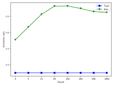
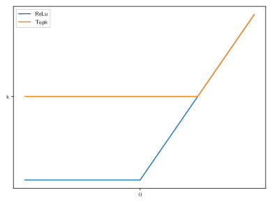
TopK VS. ReLu. In ST-SparseGCN, the ReLu function in GCN has been replaced by the TopK function. The effect of the replacement can be illustrated through Fig. 3(a), where the GCN coupled with TopK and the GCN with ReLu are compared in terms of the ratio of activated neurons during the training process. From Fig. 3(a), it can be observed that TopK greatly reduces the number of activated neurons. TopK and ReLu can also be compared through the funciton curves as shown in Fig. 3(b), from which it can be observed that it is more difficult for a neuron to be activated through the TopK activation function.
The Cost of Robustness. (Xiao, Zhong, and Zheng 2020) has proved that the computational complexiy of TopK is asymptotically , which is the same as ReLu. However, it takes more time for TopK to converge in experiments, which might originate from the spatial sparsity. Due to the spatial sparsity, only a small number of neurons can be activated, which implies that the gradient update covers only a small number of neurons in each epoch. Nevertheless, the computing cost of TopK can be reduced through the computing optimization of sparse matrix.
Attention Based Temporal Sparsification
At the first glance, it seems that temporal spasity can be realized through applying the TopK function as follows: . However, this may reduce the number of non-zero features for certain nodes, which might compromise the generalization capability as discussed previously. Furthermore, it may cause a sudden discontinuities in the model output.
To avoid the above issues, we propose an attention-based temporal sparsification mechanism, where at any epoch , for any node , its feature is assigned an attention value . This attention value will be adaptively adjusted according to the historical sparsity information of feature , namely, (). Then, the adjusted attention value is used as a weight to adjust the corresponding feature of node in the spatial sparsified GCN hidden representation (namely , as defined in Eq.(4)) so that the feature with larger sparsity value will reduce its chance to be selected by the TopK function.
Concretely, in each epoch , the attention mechanism updates the attention value of each node ’s feature based on the integration of the historical sparsity and the current sparsity of the feature (i.e. ). If integrated feature sparsity is higher than the sparsities of the other features, its attention value will be reduced accordingly.
Formally, the integrated sparsity of any feature associated with node is updated as shown in Eq.(5).
| (5) |
where is the historical sparsity of node ’s feature before epoch and is a hyper parameter that controls the decay rate of historical information. Initially, .
Based on the integrated sparsity , the attention value is updated through a smooth exponential function as shown in Eq.(6)
| (6) |
where is a hyper parameter. From Eq.(6), it can be observed that, the larger the integrated sparsity , the smaller the updated attention value , because the smooth exponential function is a monotonically decreasing function.
From Eq.( 5), it can be observed that the historical sparsity is actually independent of nodes, and so does the attention value , according to Eq.(6). Thus, Eq.( 5) and Eq.(6) can be computed only once for all nodes, from which we can obtain feature ’s historical sparsity and attention values for all nodes, namely vector and vector , respectively.
From , , we can contruct the attention mask matrix as follows.
| (7) |
Based on the attention mask matrix, the proposed ST-SparseGCN can be formalized through Eq. (8).
| (8) |
Initially, and . Eq. (8) can be desribed as follows. At epoch , in the -th layer, sparse matrix first multiplies the attention mask matrix element-wisely to temporal sparsify the feature space, so as to mitigate the Mathew effect. The sparsified matrix will be fed as input into GCN for information propagation among nodes. The GCN output is further spatially sparsified thourgh TopK activation fucntion. In the end, is passed to a fully connected layer with the softmax activation function to predict labels .
5 Experimental Evaluation
Experimental Settings
Baselines. To evaluate the robustness and effectiveness of ST-SparseGCN, experiments are performed on the deep learning framework PyTorch (Steiner et al. 2019) and the GNN extension library PyG (Fey and Lenssen 2019). The proposed defense model (ST-SparseGCN) is compared with four baselines, three of which are representative graph defense methods, on the task of node-level semi-supervised classification as follows.
-
•
GCN(Kipf and Welling 2017):GCN proposes to simplify the graph convolution using only the first order polynomial, i.e. the immediate neighborhood. By stacking multiple convolutional layers, GCN achieved the state-of- the-art performance in clean datasets.
-
•
GCN-Jaccard(Wu et al. 2019a): GCN-Jaccard utilizes the Jaccard similarity of features to prune perturbed graphs based on the assumption that the connected nodes usually show high feature similarity.
-
•
GCN-SVD(Entezari et al. 2020): GCN-SVD proposes a low-rank representation method, which can approximate the original node representation with a low-rank representation, so as to resist the adversarial attacks.
-
•
RGCN(Zhu et al. 2019): RGCN aims to defend against adversarial edges with Gaussian distributions as the latent node representation in hidden layers to absorb the negative effects of adversarial edges.
We implement the above baseline methods with refering to the implementation in DeepRobust(Li et al. 2020).
Attacker models. To validate the defensive ability of our proposed defender, we choose four representative GCN attacker models.
-
•
DICE(Waniek et al. 2018):DICE randomly selects node pairs to flip their connectivity (i.e., the removal of the existing edges and the connection of non-adjacent nodes).
-
•
Mettack(Zügner and Günnemann 2019): Mettack aims at reducing the overall performance of GNNs via meta learning. We used the attack method Meta-Self.
-
•
PGD(Xu et al. 2019b):PGD is projected gradient descent topology attack to attacking a pre-defined GNN.
-
•
Min-Max(Xu et al. 2019b): Min-max is min-max topology attack to attacking a re-trainable GNN. The minimization is optimized using the PGD method and the maximization aims to constrain the attack loss by retraining .
Parameter Setting. The following common parameters are the same for ST-SparseGCN and the baselines. The number of GCN layer is 2 and the training epochs is 200. The selected optimizer is Adam (Kingma and Ba 2015) with a fixed learning rate of 0.01. The other hyperparameters in baselines are closely followed the benchmark setup. And the hyper parameters in the ST-SparseGCN model are adjusted based on the validation set to achieve the best robust performance. Parameter sensitivity of ST-SparseGCN will be analyzed in Section 5. The final results of all experiments are obtained by averaging 5 repeated experiments. Our experiments are performed on NVIDIA RTX 2080Ti GPU.
Datasets. ST-SparseGCN is evaluated on three well-known datasets: Cora, Citeseer and Polblogs (Sen et al. 2008), where nodes represent documents and edges represent citations. The sparse bag-of-words feature vector associated with each node is the model input. Table 1 enumerates the statistics information of the datasets. The same training set, test set, and validation set from the same data set is used to fairly evaluate the performance of different models.
| Nodes | Edges | Features | Classes | |
|---|---|---|---|---|
| Cora | 2708(1 graph) | 5429 | 1433 | 7 |
| Citeseer | 3327(1 graph) | 4732 | 3703 | 6 |
| Polblogs | 1490(1 graph) | 33430 | 1490 | 2 |
Classification Performance Evaluation
In order to properly measure the impact of the perturbation, we first evaluated the performance of ST-SparseGCN and all baselines on different clean datasets. The average accuracy with standard deviation is enumerated in Table 2, which indicates that ST-SparseGCN can achieve excellent performance on clean data sets. Compared to four baselines, the superiority of ST-SparseGCN may come from the generalization capability of the temporal sparsification on the feature space.
| Cora | Citeseer | Polblogs | |
|---|---|---|---|
| GCN | 81.60.6 | 70.70.8 | 85.90.9 |
| GCN-Jaccard | 78.90.8 | 71.40.7 | 50.40.9 |
| GCN-SVD | 68.40.8 | 59.80.9 | 80.40.4 |
| RGCN | 81.10.6 | 71.40.5 | 85.30.7 |
| ST-SparseGCN | 82.20.6 | 72.00.6 | 89.10.4 |
| Dataset | Cora | Citeseer | |||||||
| Defender / Attacker | DICE | Mettack | MinMax | PGD | DICE | Mettack | MinMax | PGD | |
| GCN | 5.28 | 54.13 | 21.90 | 10.09 | 2.53 | 64.39 | 22.82 | 5.74 | |
| GCN_Jaccard | 6.82 | 38.51 | 13.18 | 17.57 | 1.12 | 53.08 | 12.16 | 4.13 | |
| GCN_SVD | 25.81 | 50.27 | 61.43 | 13.06 | 18.57 | 16.61 | 52.12 | 19.14 | |
| RGCN | 5.04 | 35.13 | 20.24 | 13.11 | 1.46 | 61.56 | 11.22 | 10.65 | |
| ST-SparseGCN | 4.33 | 48.42 | 17.44 | 7.21 | 1.92 | 60.74 | 17.96 | 4.73 | |
| ST-SparseGCN_Jaccard | 6.23 | 29.53 | 11.05 | 8.53 | 0.52 | 45.69 | 8.20 | 2.30 | |
| ST-SparseGCN_SVD | 24.87 | 47.02 | 59.13 | 13.40 | 18.22 | 15.82 | 47.82 | 19.31 | |
Defense Performance Evaluation
In the section, we evaluate the overall defense performance of the proposed ST-SparseGCN by comparing it with various defense methods under different adversarial attackers along with different perturbation sizes.
Perturbation Size. For each attacker, we increase the perturbation rate from 0 to 0.25 with a step size of 0.05. In general, the defense performance decreases along with the increase of the perturbation size. In order to concisely present the experiment results, we define a new metric to evaluate the defense performance, termed dropping rate (DR) as shown in Eq.(9).
| (9) |
where is the accuracy of GCN on clean/original graph. Dropping rate characterizes the defense performance by measuring the integration of the performance degeneration caused by attacker models and the performance remedy from the defense methods. The smaller the dropping rate, the better the defense methods. We use the mean dropping rate(mDR) to describe the overall defense performance along with different perturbation sizes.
Hybrid Defense. To illustrate that the proposed ST-SparseGCN defense methods can be complementary to the existing defense methods, we propose to integrate ST-SparseGCN with two existing defense models, namely, GCN_Jaccard and GCN_SVD, which improve GCN robustness through data preprocessing. The two integrated defense models are called ST-SparseGCN_Jaccard and ST-SparseGCN_SVD, respectively.
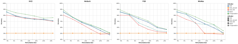
Experimental Results. The experiment results on the Cora and Citeseer datasets are enumerated in Table 3. Due to space limitation, the experiment results on the Prolblogs dataset are not included, but illustrated in Fig. 4 instead.
From Table 3, we can make the following observations: (i) the proposed ST-SparseGCN defense model or its variants (ST-SparseGCN_Jaccard and ST-SparseGCN_SVD) achieve the best defense performance under varoius attackers on all datasets, as ST-SparseGCN constructs a robust feature space in each GCN layer; (ii) the hybrid defenders (ST-SparseGCN_Jaccard and ST-SparseGCN_SVD) can improve defense performance compared with the corresponding baselines (namely GCN_Jaccard and GCN_SVD) alone in most cases, which implies that our proposed defender ST-SparseGCN is complementary to the existing defenders, because ST-SparseGCN intends defend the adversarial attacks from the perspective of sparsification in feature space, which is complementary to most of the existing defense methods; (iii) none of the existing non-hybrid graph defenders (including the ST-SparseGCN alone) can perform best under all attackers on all datasets. This phenomenon may originate from the fact that the success of adversarial attacks comes from various aspects of the GCN model. Thus, the hybrid defense models may deserve further exploration.
Fig. 4 summaries the performance results under different attackers along with varied perturbation sizes on the Polblogs dataset. The results show that ST-SparseGCN again consistently achieves better performance than all the baselines, which demonstrates the superiority of the proposed ST-SparseGCN model. The experiment results shown in Table 3 and Fig. 4 have illustrated that our defender can improve defense performance under all attackers on all datasets. It is worth to note that ST-SparseGCN does not rely on any prior knowledge of any particular adversarial attack method. The advantage of ST-Sparse might lie in that it can construct a robust feature space, which can be effectively against various adversarial attacks.
SparseGCN and Dropout
In the section, we compare the generalization performance and robustness of ST-Sparse and Dropout through experiments. Table 4 demonstrates both dropout and ST-Sparse can improve the generalization ability of the model, and ST-Sparse is even better. In terms of robustness, ST-Sparse performs better than Dropout in the face of attacker. In addition, Dropout combined with ST-Sparse will damage the performance of the model. This phenomenon may be the random inactivation of Dropout will damage the ability to preferentially select features in ST-Sparse.
| GCN | ST-SparseGCN | |
|---|---|---|
| Clean | 81.50.6 | 82.70.6 |
| +Dropout | 81.70.7 | 81.50.6 |
| +Attacker | 65.60.9 | 69.60.6 |
| +Dropout+Attacker | 66.90.7 | 68.30.8 |
-
1
The dataset is Cora. The attacker is Mettack. The perturbation size is 0.05.
-
2
The results are averaged five times.
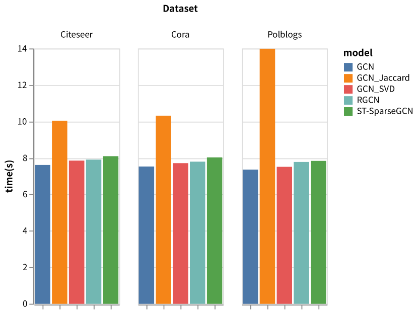
Time Complexity
We conduct several experiments on datasets-model pairs mentioned above to report the runtime of a whole training procedure for 200 epochs obtained on a single NVIDIA RTX 2080 Ti (cf. Fig. 5). Thanks to the ability to quickly process sparse data in the PYG framework, the time overhead between models is basically the same. Among them, GCN_Jaccard takes the most time because its data preprocessing process is very slow.
Ablation Study and Parameter Analysis
In this section, we evaluate the maginal effect of the temporal sparsity, spatial sparsity, and the dimension on the accuracy and robustness of ST-SparseGCN. The performance evaluated on clean and perturbed datasets are shown separately. Due to space limitation, we only show the experiment results on the Cora dataset under the Mettack with a perturbation size of 0.05. The experiments on the other datasets exhibit similar patterns, which are included in the supplementary material.
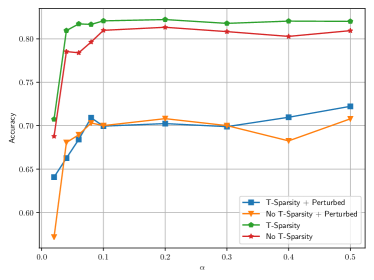
In the experiments, the extent of the spatial sparsity is controlled by the spatial sparse ratio . Fig. 6(a) shows that the influence of the temporal sparsity and the Mettack along with the increasing sparse ratio from to , where T-Sparsity and Perturbed represent the temporal sparsity and the perturbation from the Mettack, respectively. From Fig. 6(a), by comparing the performance of the models with and without temporal spasity, it can be osberved that temporal sparsity can effectively improve the ST-SparseGCN’s classification performance on both the clean graphs and the perturbed graphs. This illustrates the benefits of the temporal sparsity, which can not only increase the model’s generalization capability (from the performance improvement on the clean graphs), but also improve the model’s defense performance (from the performance improvement on the perturbed graphs).
It can also be inferred from Fig. 6(a) that, when the spatial sparsity ratio varies from a small value (0.02) to a relative larger value (0.08), both the models with and without temporal sparsity show significant performance improvement. Thus, this illustrates the necessity of spatial sparsity. Moreover, when is larger than 0.08, the accuracy of the ST-SparseGCN remains basically unchanged. However, a very small will degrade the performance, probably because the number of non-zero features is not enough to distinguish different categories for node classificaiton task.
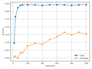
Fig. 6(b) illustrates the impact of the dimension on the performance. It is can be observed that whether it is the clean dataset or the perturbed dataset, the performance is drastically reduced when reduced to a small value. On the other hand, when increases to a certain level, the performance almost remains stable. This illustrates that there exists an appropriate value for . The results also illustrate that the high-dimensional space can enable the GCN model to have more robust performance in case of the perturbation incurred by the attackers.
6 Conclusion
Although the GNN models have emerged rapidly, they still suffer the adversarial attack problem. Unlike the current works, which defend the attack on certain specific scenarios, this paper intends to universally address the attack problem. The proposed ST-Sparse mechanism is similar to the Dropout regularization technique in spirit, as it can provide a general adversarial defense layer, which can be readily integrated into numerous GNN variants. Meanwhile, ST-Sparse can also ensure both robust generalization and ordinary generalization. To evaluate the ST-Sparse’s effectiveness, we conduct intensive experiments. The experiment results show that, in the face of four representative attack methods on three representative datasets with different levels of perturbation, ST-SparseGCN outperforms three representative defense methods.
References
- Ahmad and Scheinkman (2019) Ahmad, S.; and Scheinkman, L. 2019. How Can We Be So Dense? The Benefits of Using Highly Sparse Representations. In ICML 2019 Workshop on Uncertainty & Robustness in Deep Learning. URL http://arxiv.org/abs/1903.11257.
- Bojchevski and Günnemann (2019) Bojchevski, A.; and Günnemann, S. 2019. Certifiable Robustness to Graph Perturbations. In Advances in Neural Information Processing Systems 32, 8319–8330. Curran Associates, Inc. URL http://papers.nips.cc/paper/9041-certifiable-robustness-to-graph-perturbations.pdf.
- Chen et al. (2019) Chen, J.; Wu, Y.; Lin, X.; and Xuan, Q. 2019. Can Adversarial Network Attack be Defended? CoRR abs/1903.05994. URL http://arxiv.org/abs/1903.05994.
- Cosentino et al. (2019) Cosentino, J.; Zaiter, F.; Pei, D.; and Zhu, J. 2019. The Search for Sparse, Robust Neural Networks. arXiv preprint arXiv:1912.02386 (NeurIPS). URL http://arxiv.org/abs/1912.02386.
- Dai et al. (2018) Dai, H.; Li, H.; Tian, T.; Xin, H.; Wang, L.; Jun, Z.; and Le, S. 2018. Adversarial attack on graph structured data. In 35th International Conference on Machine Learning, ICML 2018, volume 3, 1799–1808. ISBN 9781510867963.
- Entezari et al. (2020) Entezari, N.; Al-Sayouri, S. A.; Darvishzadeh, A.; and Papalexakis, E. E. 2020. All you need is Low (rank): Defending against adversarial attacks on graphs. WSDM 2020 - Proceedings of the 13th International Conference on Web Search and Data Mining 169–177. doi:10.1145/3336191.3371789.
- Feng et al. (2019) Feng, F.; He, X.; Tang, J.; and Chua, T.-S. 2019. Graph Adversarial Training: Dynamically Regularizing Based on Graph Structure. IEEE Transactions on Knowledge and Data Engineering 1–1. ISSN 1041-4347. doi:10.1109/tkde.2019.2957786.
- Fey and Lenssen (2019) Fey, M.; and Lenssen, J. E. 2019. Fast Graph Representation Learning with PyTorch Geometric. In ICLR Workshop on Representation Learning on Graphs and Manifolds, 1, 1–9. URL http://arxiv.org/abs/1903.02428.
- Guo et al. (2018) Guo, Y.; Zhang, C.; Zhang, C.; and Chen, Y. 2018. Sparse DNNs with improved adversarial robustness. Advances in Neural Information Processing Systems 2018-Decem(NeurIPS): 242–251. ISSN 10495258.
- Jin et al. (2020) Jin, W.; Li, Y.; Xu, H.; Wang, Y.; and Tang, J. 2020. Adversarial Attacks and Defenses on Graphs: A Review and Empirical Study. arXiv preprint arXiv:2003.00653 URL http://arxiv.org/abs/2003.00653.
- Kingma and Ba (2015) Kingma, D. P.; and Ba, J. L. 2015. Adam: A method for stochastic optimization. 3rd International Conference on Learning Representations, ICLR 2015 - Conference Track Proceedings 1–15.
- Kipf and Welling (2017) Kipf, T. N.; and Welling, M. 2017. Semi-supervised classification with graph convolutional networks. In 5th International Conference on Learning Representations, ICLR 2017 - Conference Track Proceedings, 1–14.
- Li et al. (2020) Li, Y.; Jin, W.; Xu, H.; and Tang, J. 2020. DeepRobust: A PyTorch Library for Adversarial Attacks and Defenses. arXiv preprint arXiv:2005.06149 .
- Sen et al. (2008) Sen, P.; Namata, G. M.; Bilgic, M.; Getoor, L.; Gallagher, B.; and Eliassi-Rad, T. 2008. Collective classification in network data. AI Magazine 29(3): 93–106. ISSN 07384602. doi:10.1609/aimag.v29i3.2157.
- Srivastava et al. (2014) Srivastava, N.; Hinton, G.; Krizhevsky, A.; Sutskever, I.; and Salakhutdinov, R. 2014. Dropout: a simple way to prevent neural networks from overfitting. The journal of machine learning research 15(1): 1929–1958.
- Steiner et al. (2019) Steiner, B.; Devito, Z.; Chintala, S.; Gross, S.; Paszke, A.; Massa, F.; Lerer, A.; Chanan, G.; Lin, Z.; Yang, E.; Desmaison, A.; Tejani, A.; Kopf, A.; Bradbury, J.; Antiga, L.; Raison, M.; Gimelshein, N.; Chilamkurthy, S.; Killeen, T.; Fang, L.; and Bai, J. 2019. PyTorch: An Imperative Style, High-Performance Deep Learning Library. NeuroIPS (NeurIPS).
- Sun et al. (2018) Sun, L.; Wang, J.; Yu, P. S.; and Li, B. 2018. Adversarial Attack and Defense on Graph Data: A Survey. arXiv preprint arXiv:1812.10528 URL http://arxiv.org/abs/1812.10528.
- Tsipras et al. (2019) Tsipras, D.; Santurkar, S.; Engstrom, L.; Turner, A.; and Madry, A. 2019. Robustness may be at odds with accuracy. In 7th International Conference on Learning Representations, ICLR 2019, 1–24.
- Wang et al. (2019) Wang, S.; Chen, Z.; Ni, J.; Yu, X.; Li, Z.; Chen, H.; and Yu, P. S. 2019. Adversarial Defense Framework for Graph Neural Network. arXiv preprint arXiv:1905.03679 URL http://arxiv.org/abs/1905.03679.
- Waniek et al. (2018) Waniek, M.; Michalak, T. P.; Wooldridge, M. J.; and Rahwan, T. 2018. Hiding individuals and communities in a social network. Nature Human Behaviour 2(2): 139–147. ISSN 23973374. doi:10.1038/s41562-017-0290-3.
- Wu et al. (2019a) Wu, H.; Wang, C.; Tyshetskiy, Y.; Docherty, A.; Lu, K.; and Zhu, L. 2019a. Adversarial examples for graph data: Deep insights into attack and defense. IJCAI International Joint Conference on Artificial Intelligence 2019-August: 4816–4823. ISSN 10450823. doi:10.24963/ijcai.2019/669.
- Wu et al. (2019b) Wu, Z.; Pan, S.; Chen, F.; Long, G.; Zhang, C.; and Yu, P. S. 2019b. A Comprehensive Survey on Graph Neural Networks. IEEE Transactions on Neural Networks and Learning Systems XX(Xx): 1–22. URL http://arxiv.org/abs/1901.00596.
- Xiao, Zhong, and Zheng (2020) Xiao, C.; Zhong, P.; and Zheng, C. 2020. Enhancing Adversarial Defense by k-Winners-Take-All. In International Conference on Learning Representations. URL https://openreview.net/forum?id=Skgvy64tvr.
- Xu et al. (2019a) Xu, H.; Ma, Y.; Liu, H.; Deb, D.; Liu, H.; Tang, J.; and Jain, A. K. 2019a. Adversarial Attacks and Defenses in Images, Graphs and Text: A Review URL http://arxiv.org/abs/1909.08072.
- Xu et al. (2019b) Xu, K.; Chen, H.; Liu, S.; Chen, P. Y.; Weng, T. W.; Hong, M.; and Lin, X. 2019b. Topology attack and defense for graph neural networks: An optimization perspective. In IJCAI International Joint Conference on Artificial Intelligence, volume 2019-Augus, 3961–3967. ISBN 9780999241141. ISSN 10450823. doi:10.24963/ijcai.2019/550.
- Zhang, Hossain Khan, and Coates (2019) Zhang, Y.; Hossain Khan, S.; and Coates, M. 2019. Comparing and Detecting Adversarial Attacks for Graph Deep Learning. In ICLR 2019 Workshop: Representation Learning on Graphs and Manifolds, 1–7. URL https://www.kdd.in.tum.de/research/nettack/.
- Zhang, Cui, and Zhu (2020) Zhang, Z.; Cui, P.; and Zhu, W. 2020. Deep Learning on Graphs: A Survey. IEEE Transactions on Knowledge and Data Engineering 1–1. ISSN 1041-4347. doi:10.1109/tkde.2020.2981333.
- Zheng et al. (2020) Zheng, C.; Zong, B.; Cheng, W.; Song, D.; Ni, J.; Yu, W.; Chen, H.; and Wang, W. 2020. Robust Graph Representation Learning via Neural Sparsification . In Proceedings of ICML 2020.
- Zhou et al. (2018) Zhou, J.; Cui, G.; Zhang, Z.; Yang, C.; Liu, Z.; Wang, L.; Li, C.; and Sun, M. 2018. Graph Neural Networks: A Review of Methods and Applications 1–22. URL http://arxiv.org/abs/1812.08434.
- Zhu et al. (2019) Zhu, D.; Cui, P.; Zhang, Z.; and Zhu, W. 2019. Robust graph convolutional networks against adversarial attacks. In Proceedings of the ACM SIGKDD International Conference on Knowledge Discovery and Data Mining, 1399–1407. ISBN 9781450362016. doi:10.1145/3292500.3330851.
- Zügner, Akbarnejad, and Günnemann (2018) Zügner, D.; Akbarnejad, A.; and Günnemann, S. 2018. Adversarial attacks on neural networks for graph data. In Proceedings of the ACM SIGKDD International Conference on Knowledge Discovery and Data Mining, 2847–2856. ISBN 9781450355520. doi:10.1145/3219819.3220078.
- Zügner and Günnemann (2019) Zügner, D.; and Günnemann, S. 2019. Adversarial attacks on graph neural networks via meta learning. In 7th International Conference on Learning Representations, ICLR 2019, 1–15.