SpComp: A Sparsity Structure-Specific Compilation of Matrix Operations
Abstract.
Sparse matrix operations involve a large number of zero operands which makes most of the operations redundant. The amount of redundancy magnifies when a matrix operation repeatedly executes on sparse data. Optimizing matrix operations for sparsity involves either reorganization of data or reorganization of computations, performed either at compile-time or run-time. Although compile-time techniques avert from introducing run-time overhead, their application either is limited to simple sparse matrix operations generating dense output and handling immutable sparse matrices or requires manual intervention to customize the technique to different matrix operations.
We contribute a sparsity structure-specific compilation technique, called SpComp, that optimizes a sparse matrix operation by automatically customizing its computations to the positions of non-zero values of the data. Our approach neither incurs any run-time overhead nor requires any manual intervention. It is also applicable to complex matrix operations generating sparse output and handling mutable sparse matrices. We introduce a data-flow analysis, named Essential Indices Analysis, that statically collects the symbolic information about the computations and helps the code generator to reorganize the computations. The generated code includes piecewise-regular loops, free from indirect references and amenable to further optimization.
We see a substantial performance gain by SpComp-generated Sparse Matrix-Sparse Vector Multiplication (SpMSpV) code when compared against the state-of-the-art TACO compiler and piecewise-regular code generator. On average, we achieve performance gain against TACO and performance gain against the piecewise-regular code generator. When compared against the CHOLMOD library, SpComp generated sparse Cholesky decomposition code showcases performance gain on average.
1. Introduction
Sparse matrix operations are ubiquitous in computational science areas like circuit simulation, power dynamics, image processing, structure modeling, data science, etc. The presence of a significant amount of zero values in the sparse matrices makes a considerable amount of computations, involved in the matrix operation, redundant. Only the computations computing non-zero values remain useful or non-redundant.
In simulation-like scenarios, a matrix operation repeatedly executes on sparse matrices whose positions or indices of non-zero values, better known as sparsity structures, remain unchanged although the values in these positions may change. For example, Cholesky decomposition in circuit simulation repeatedly decomposes the input matrix in each iteration until the simulation converges. The input matrix represents the physical connections of the underlying circuit and thus, remains unchanged throughout the simulation, although the values associated with the connections may vary. In such a scenario, the redundant computations caused by computing zero values get multi-fold and therefore, it is prudent to claim substantial performance benefits by altering the execution based on the fixed sparsity structure.
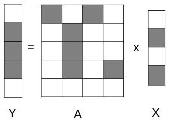
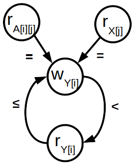
The state-of-the-art on avoiding redundant computations categorically employs either (a) reorganizing sparse data in a storage format such that the generic computations operate only on the non-zero data or (b) reorganizing computations to restrict them to non-zero data without requiring any specific reorganization of the data. Figure 1 demonstrates the avoidance of redundant computations of Sparse Matrix-Sparse Vector Multiplication operation (SpMSpV) by reorganizing data and reorganizing computations. The operation multiplies sparse matrix to sparse vector and stores the result in the output sparse vector . Figure 1(b) presents the computations on reorganized matrix stored using Compressed Sparse Row (CSR) format. As a result, the non-zero values are accessed using indirect reference . On the contrary, Figure 1(c) presents the reorganized SpMSpV computations customized to the positions of the non-zero elements of . Clearly, reorganized computations result in direct references and a minimum number of computations.
Approaches reorganizing computations avoid redundant computations by generating sparsity structure-specific execution. This can be done either at run-time or at compile-time. Run-time techniques like inspection-execution (Mirchandaney et al., 1988) exploit the memory traces at run-time. The executor executes the optimized schedule generated by the inspector after analyzing the dependencies of the memory traces. Even with compiler-aided supports, the inspection-execution technique incurs considerable overhead at each instance of the execution and thus increases the overall runtime, instead of reducing it to the extent achieved by compile-time optimization approaches.
Instead of reorganizing access to non-zero data through indirections or leaving its identification to runtime, it is desirable to symbolically identify the non-zero computations at compile-time and generate code that is aware of the sparsity structure. The state-of-the-art that employs a static approach can be divided into two broad categories:
-
•
A method could focus only on the sparsity structure of the input, thereby avoiding reading the zero values in the input wherever possible. This approach works only when the output is dense and the memory trace is dominated by the sparsity structure of a single sparse data. Augustine et al. (Augustine et al., 2019) and Rodríguez et al. (Pouchet and Rodríguez, 2018) presented a trace-based technique to generate sparsity structure-specific code for matrix operations resulting in dense data.
-
•
A method could focus on the sparsity structure of the output, thereby statically computing the positions of non-zero elements in the output from the sparsity structures of the input. This approach works when the output is sparse or the memory trace is dominated by the sparsity structures of multiple sparse data. This can also handle changes in the sparsity structure of the input, caused by the fill-in elements in mutable cases.
Such a method can involve a trace-based technique that simply unwinds a program and parses it based on the input to determine the sparsity structure of the output. Although sounds simple, the complexity of this technique bounds to the computations involved in the matrix operation and size of the output, making it a resource-consuming and practically intractable for complex matrix operations and large-sized inputs.
Alternatively, a graph-based technique like Symbolic analysis (Davis et al., 2016) uses matrix operation-specific graphs and graph algorithms to deduce the sparsity structure of the output. Cheshmi et al. (Cheshmi et al., 2017, 2018, 2018) apply this analysis to collect symbolic information and enables further optimization. The complexity of this technique is bound to the number of non-zero elements of the output, instead of its size, making it significantly less compared to the compile-time trace-based technique. However, the Symbolic analysis is matrix-operation specific, so the customization of the technique to different matrix operations requires manual effort.
We propose a data-flow analysis-based technique, named Sparsity Structure Specific Compilation (SpComp), that statically deduces the sparsity structure of the output from the sparsity structure of the input. Our method advances the state-of-the-art in the following ways.
-
•
In comparison to the run-time approaches, our method does not depend on any run-time information, making it a purely compile-time technique.
- •
-
•
In comparison to the compile-time trace-based technique, the complexity of our method is bound to the number of non-zero elements present in the output which is significantly less than the size of the output, making it a tractable technique.
-
•
In comparison to the Symbolic analysis (Davis et al., 2016), our method is generic to any matrix operation, without the need for manual customization.
SpComp takes a program performing matrix operation on dense data and sparsity structures of the input sparse data to compute the sparsity structure of the output and derive the non-redundant computations. The approach avoids computing zero values in the output wherever possible, which automatically implies avoiding reading zero values in the input wherever possible. Since it is driven by discovering the sparsity structure of the output, it works for matrix operations producing sparse output and altering the sparsity structures of the input. From the derived symbolic information, SpComp generates the sparsity structure-specific code, containing piecewise-regular and indirect reference-free loops.
|
|
|||||||||||||||||
| (a) | (b) |
Example 0.
Figure 2(a) shows the inputs to the SpComp; (i) the code performing forward Cholesky decomposition of symmetric positive definite dense matrix and (ii) the initial sparsity structure of the input matrix selected from the Suitesparse Matrix Collection (Davis, 2023a). Figure 2(b) illustrates the output of SpComp; (i) fill-in elements of along with the initial sparsity structure generate the sparsity structure of the output matrix. (ii) Cholesky decomposition code, customized to sparse matrix.
Note that, although there exists a read-after-write (true) dependency from statement to statement in the program present in Figure 2(ai), a few instances of hoist above in the execution due to spurious dependencies produced by zero-value computations.
The rest of the paper is organized as follows. Section 2 provides an overview of SpComp. Section 3 describes the first step of SpComp, which identifies the indices involving the computations leading to non-zero values through a novel data flow analysis called Essential Indices Analysis. Section 4 explains the second step which generates the code. Section 5 presents the empirical results. Section 6 describes the related work. Section 7 concludes the paper.
2. An Overview of SpComp
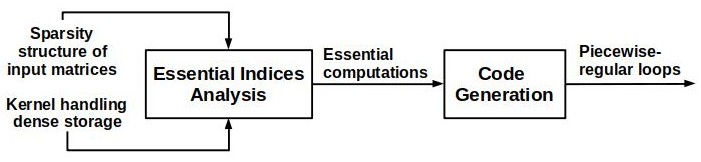 |
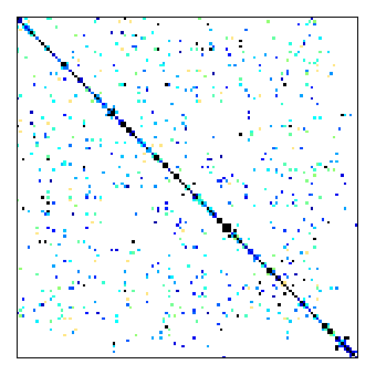
As depicted in Figure 3, SpComp has two modules performing (a) essential indices analysis and (b) code generation. The essential indices analysis module constructs an Access Dependence Graph (ADG) from the program and performs a data flow analysis, named Essential Indices Analysis. The analysis effectively identifies the essential data indices of the output matrix and essential iteration indices of the iteration space. Essential data indices identify the indices of non-zero elements which construct the underlying sparse data storage beforehand, without requiring any modification during run-time. Essential iteration indices identify the iteration points in the iteration space that must execute to compute the values of the non-zero elements and facilitate the generation of piecewise-regular loops.
| Fill-in | Essential iteration indices of | |||
|---|---|---|---|---|
| elements of A | ||||
Example 0.
For our motivating example in Figure 2, the essential indices analysis generates the essential data indices and essential iteration indices for statements , , , and as shown in Figure 4. Note that this analysis is an abstract interpretation of the program with abstract values, we do not compute the actual expressions with concrete values. The input sparse matrix 494_bus is represented by the array A in the code, which is both the input and the output matrix.
The essential data indices of the output matrix comprise the indices of non-zero elements of the input matrix and the fill-in elements denoting the indices whose values are zero in the input but become non-zero in the output. 111The converse (i.e. a non-zero value of an index in the input becoming zero at the same index in the output) is generally not considered explicitly in such computations and are performed by default. Fill-in element identifies whose value changes from zero to non-zero during the execution of the program. The essential iteration index of statement identifies as a statement instance that should be executed to preserve the semantics of the program.
At first, the code generation module finds the timestamps of the essential iteration indices and lexicographically orders them to construct the execution trace, without any support for the out-of-order execution. Then it simply finds the pieces of execution trace that can be folded back into regular loops. The module also constructs the memory access trace caused by the execution order and mines the access patterns for generating the subscript functions of the regular loops. Note that, the generated code keeps the if conditions to avoid division by zero during execution.
Example 0.
The execution trace is generated by the lexicographic order of the timestamps where represents iteration index of statement . It is evident that the piece of execution trace can be folded back in a loop. The corresponding memory access trace creates a one-dimensional subscript function . represents the one-dimensional array storing the non-zero values of and represents the positions of , , and in the sparse data storage. The generated code snippet is presented in Figure 2(bii).
3. Essential Indices Analysis
In sparse matrix operations, we assume that the default values of matrix elements are zero. The efficiency of a sparse matrix operation lies in avoiding the computations leading to zero or default values. We call such computations as default computations. Computations leading to non-zero values are non-default computations.
We refer to the data indices of all input and output matrices holding non-zero values as essential data indices. As mentioned before, we have devised a data flow analysis technique called Essential Indices analysis that statically computes the essential data indices of output matrices from the essential data indices of input matrices. We identify all the iteration indices of the loop computing non-default computations as essential iteration indices. Here we describe the analysis by defining Access Dependence Graph as the data flow analysis graph in Subsection 3.1, the domain of data flow values in Subsection 3.2, and the transfer functions with the data flow equations in Subsection 3.3. Finally, we prove the correctness of the analysis in Subsection 3.4.
3.1. Access Dependence Graph
Conventionally, data flow analysis uses the Control Flow Graph (CFG) of a program to compute data flow information at each program point. However, CFG is not suitable for our analysis because the set of information computed over CFG of a loop is an over-approximation of the union of information generated in all iterations. Thus, information gets conflated across all iterations, and no distinction exists between the fact that information generated in -th iteration cannot be used in iterations if .
SpComp accepts static control parts (SCoP) (Benabderrahmane et al., 2010; Bastoul et al., 2004) of a program which is a sequence of perfectly and imperfectly nested loops where loop bounds and subscript functions are affine functions of surrounding loop iterators and parameters. For essential indices analysis, we model SCoP in the form of an Access Dependence Graph (ADG). ADG captures (a) data dependence, i.e., accesses of the same memory locations, and (b) data flow, i.e., the flow of a value from one location to a different location. They are represented by recording flow, anti and output data dependencies, and the temporal order of read and write operations over distinct locations. This modeling of dependence is different from the modeling of dependence in a Data Dependence Graph (DDG) (Kennedy and Allen, 2001; Banerjee, 1988) that models data dependencies among loop statements which are at a coarser level of granularity.
ADG captures dependencies among access operations which are at a finer level of granularity compared to loop statements. Access operations on concrete memory locations, i.e., the locations created at run-time, are abstracted by access operations on abstract memory locations that conflate concrete memory locations accessed by a particular array access expression. For example, the write access operations on concrete memory locations at statement in Figure 2(a) are accessed by the access expression .
ADG handles the affine subscript function of the form , assuming and be constants and be an iteration index. A set of concrete memories read by an affine array expression at statement is denoted by an access operation , where and denote lower and upper bounds of regular or irregular loops. Similarly, a set of concrete memories written by the same array expression at statement is denoted by an access operation . Note that, the bounds on the iteration indices become implicit to the access operation. For code generation, we concretize an abstract location into concrete memory locations , etc. using the result of essential indices analysis as explained in Section 3.3.
ADG captures the temporal ordering of access operations using edges annotated with a dependence direction that models the types of dependencies. Dependence direction , and model flow, anti and output data dependencies, whereas dependence direction captures the data flow between distinct memory locations. Note that dependence direction is not valid as the source of a dependency can not be executed after the target.
|
|
||
| (a) | (b) |
Example 0.
Consider statement in Figure 5(a). It is evident that there is an anti dependency from the read access of , denoted as , to write access of , denoted as . The anti-dependency is represented by an edge where the direction of the edge indicates the ordering and the edge label indicates that it is an anti-dependency.
Similarly, there is a flow dependency from to . This is represented by an edge where direction of the edge indicates the ordering and the edge label denotes the flow dependency.
The data flow from to and to are denoted by the edges and respectively where the directions indicate the ordering and the edge labels indicate that these are data flow.
Each vertex in the ADG is called an access node, and the entry and exit points of each access node are access points. Distinctions between entry and exit access points are required for formulating transfer functions and data flow equations in Section 3.3.
Formally, ADG captures the temporal and spatial properties of data flow. Considering every statement instance as atomic in terms of time, the edges in an ADG have associated temporal and spatial properties, as explained below.
Let and respectively denote read and write access nodes.
-
•
For edge where , edge label implies that executes in the same statement instance as and captures data flow.
-
•
For edge where , edge label implies that executes either in the same statement instance as or in a statement instance executed later and captures anti dependencies.
-
•
For edge where , edge label implies that executes in a statement instance executed after the execution of and captures flow dependencies.
-
•
For edge where , edge label implies that executes in a statement instance executed after the execution of and captures output dependencies.
3.2. Domain of Data Flow Values
Let the set of data indices of an -dimensional matrix of size be represented as where has data size at dimension . Here where vector represents a data index of matrix . If is sparse in nature then is an essential data index if . The set of essential data indices of sparse matrix is represented as such that . For example, of a -dimensional matrix of size is , , , , , , , , , the set of all data indices of . If is sparse with non-zero elements at , , and then = . Thus .
In this analysis, we consider the union of all data indices of all input and output matrices as data space . The union of all essential data indices of all input and output matrices is considered as the domain of data flow values such that . For our analysis each essential data index of is annotated with the name of the origin matrix. For an -dimensional matrix each essential data index thus represents an dimensional vector where the -th position holds the name of the matrix, . For example, in the matrix-vector multiplication of Figure 5(a), let , and . Thus, the domain of data flow values is .
In the rest of the paper data index is denoted as for convenience. The value at data index is abstracted as either zero (Z) or nonzero (NZ) based on the concrete value at . Note that the domain of concrete values, , at each data index is a power set of , which is the set of real numbers. Our approach abstracts the concrete value at each by defined as follows.
| (1) |
The domain of values at each data index forms a component lattice , where and represents the partial order.
A data index is called essential if . As the data flow value at any access point holds the set of essential data indices such that , the data flow lattice is thus represented as where partial order is a superset relation.
3.3. Transfer Functions
This section formulates the transfer functions used to compute the data flow information of all data flow variables and presents the algorithm performing Essential Indices Analysis. For an ADG, , the data flow variable captures the data flow information generated by each access node , and the data flow variable captures the data flow information generated at the exit of each node .
Let be the initial set of essential data indices that identifies the indices of non-zero elements of input matrices. In Essential Indices Analysis, is defined as follows.
| (2) |
denotes the set of predecessors of each node in the access dependence graph.
Equation 2 initializes to for access node that does not have any predecessor. Read access nodes do not generate any essential data indices; they only combine the information of their predecessors. A write access node typically computes the arithmetic expression associated with it and generates a set of essential data indices as . Finally, is combined with the out information of its predecessors to compute of write node .
Here we consider the statements associated with write access nodes and admissible in our analysis. They are of the form , and where is copy assignment, uses unary operation and uses binary operation. Here , , and are data indices.
Instead of concrete values, the operations execute on abstract values . Below we present the evaluation of all valid expressions on abstract values. Note that the unary operations negation, square root, etc. return the same abstract value as input.222Unary operations such as floor, ceiling, round off, truncation, saturation, shift etc. that may change the values are generally not used in sparse matrix operations. Thus evaluation effect of expressions and are combined into the following.
| (3) |
We consider the binary operations addition, subtraction, multiplication, division, and modulus. Thus the evaluation of expression is defined as follows for the aforementioned arithmetic operations.
-
•
If is addition or subtraction then
(4) -
•
If is multiplication then
(5) -
•
If is division or modulus then
(6)
Note that, the addition and subtraction operations may result in zero values due to numeric cancellation while operating in the concrete domain. This means cval(d) can be zero when and are non-zeroes. In this case, our abstraction over-approximates as , which is a safe approximation.
Division or modulus by zero is an undefined operation in the concrete domain and is protected by the condition on the denominator value . We protect the same in the abstract domain by the condition , as presented in Equation 6. Although handled, the conditions are still part of the generated code to preserve the semantic correctness of the program. For example, the if conditions in the sparsity structure-specific Cholesky decomposition code in Figure 2(bii) preserve the semantic correctness of the program by prohibiting the divisions by zero values in the concrete domain. In this paper, we limit our analysis to simple arithmetic operations. However, similar abstractions could be defined for all operations by ensuring that no possible non-zero result is abstracted as zero.
Now that we have defined the abstract value computations for different arithmetic expressions, below we define , which generates the set of essential data indices for write access node .
| (7) |
In the case of a binary operation, predecessor node may or may not be equal to predecessor node .
The objective is to compute the least fixed point of Equation 2. Thus the analysis must begin with the initial set of essential data indices . The data flow variables are set to initial values and the analysis iteratively computes the equations until the fixed point is reached. If we initialize with something else the result would be different and it would not be the least fixed point. Once the solution is achieved the analysis converges.
Essential indices analysis operates on finite lattices and is monotonic as it only adds the generated information in each iteration. Thus, the analysis is bound to converge on the fixed point solution. The existence of a fixed point solution is guaranteed by the finiteness of lattice and monotonicity of flow functions.
| Let, | ||||
| Essential indices analysis | ||||
| Data flow variable | Initialization | Iteration | Iteration | Iteration |
Example 0.
Figure 6 demonstrates essential indices analysis for the sparse matrix-sparse vector multiplication operation. It takes the ADG from Figure 5(b) and performs the data flow analysis based on the sparsity structures of input matrix and input vector as depicted in Figure 1(a). Let, be , , , , , , , . The gen and out information of access nodes , , and are presented in tabular form for convenience. Out information of all read nodes are initialized to , whereas the out information of write node is initialized to .
In iteration , is where . Thus becomes such that . In iteration the out information of propagates along with edge and sets to . Finally at iteration the analysis reaches the fixed point solution and converges.
Data flow variable is introduced to accumulate at each write node required by a post-analysis step computing set of essential iteration indices from the set of essential data indices.
| (8) |
In the current example is initialized to . It accumulates generated at each iteration, finally resulting as .
denotes the fill-in elements of the output sparse matrix and is computed as follows.
| (9) |
The initial essential data indices and the fill-in elements together compute the final essential data indices that captures the sparsity structure of the output matrix.
| (10) |
In the current example, is computed as . As does not contain any initial essential data index of , becomes same as .
The set of essential iteration indices is computed from the set of essential data indices. Let of size be the iteration space of dimension of a loop having depth where the loop at depth has iteration size . Thus, where vector is an iteration index. For convenience, here on we identify as . The iteration index at which non-default computations are performed is called the essential iteration index. The set of all essential iteration indices is denoted as such that .
For each essential data index there exists a set of essential iteration indices at which the corresponding non-default computations resulting occur. We introduce such that results where and . Data flow variable is introduced to capture the set of essential iteration indices corresponding to the data indices . Thus,
| (11) |
In the current example is computed as .
Finally, the set of all essential iteration indices is computed as
| (12) |
|
Input :
(a) ADG, , of a matrix operation containing access nodes and edges,
(b) Intial set of essential data indices of input matrices.
Output :
(a) Set of essential data indices of output matrix,
(b) Set of essential iteration indices .
1
2, initialize to where
3
4
do
5
Pick and remove node from
6
9
if then
10
11 end if
12
13while ;
return
|
Algorithm 1 presents the algorithm for essential indices analysis. Line number initializes . Line number sets the work list, , to the nodes of the ADG. Lines perform the data flow analysis by iterating over the ADG until the analysis converges. At an iteration, each node is picked and removed from the work list and , , and are computed. If the newly computed differs from its old value, the node is pushed back to the work list. The process iterates until the work list becomes empty. Post convergence, and are computed in line number and the values are returned.
The complexity of the algorithm depends on the number of iterations and the amount of workload per iteration. The number of iterations is derived from the maximum depth of the ADG, i.e., the maximum number of back edges in any acyclic path derived from the reverse postorder traversal of the graph. Therefore, the total number of iterations is , where the first iteration computes the initial values of for all the nodes in the ADG, iterations backpropagate the values of , and the last iteration verifies the convergence. In the current example, the reverse postorder traversal of the ADG produces the acyclic path , containing a single back edge . Therefore, the total number of iterations becomes .
The amount of workload per iteration is dominated by the computation of . In the case of a binary operation, the complexity of is bound to , where , , and . In the case of assignment and unary operations, the complexity of is bound to .
3.4. Correctness of Essential Indices Analysis
The following claims are sufficient to prove the correctness of our analysis.
-
•
Claim 1: Every essential data index will always be considered essential.
-
•
Claim 2: A data index considered essential will not become non-essential later.
Before reasoning about the aforementioned claims we provide an orthogonal lemma to show the correctness of our abstraction.
Lemma 0.
Our abstraction function is sound.
Proof.
Our abstraction function maps the concrete value domain of to the abstract value domain . in the concrete domain maps to in the abstract domain and all other elements map to . Now to guarantee the soundness of one needs to prove that the following condition (Møller and Schwartzbach, 2015) holds.
| (13) |
where is an element in the concrete domain, is an auxiliary function in the abstract domain, and is the corresponding function in the concrete domain. This condition essentially states that the evaluation of function in the abstract domain should overapproximate the evaluation of function in the concrete domain. We prove the above condition for evaluation of each admissible statement in the following lemmas. ∎
Lemma 0.
For copy assignment statement ,
.
Lemma 0.
For statement using unary operation ,
.
Lemma 0.
For statement using binary operation ,
.
Proof.
Let and where and are non-zero elements in the concrete domain and where represents abstract non-zero value.
| statement | concrete evaluation | abstract evaluation |
|---|---|---|
| , = | , |
Claim 1 primarily asserts that an essential data index will never be considered non-essential. We prove it using induction on the length of paths in the access dependence graph.
Proof of Claim 1.
Let be the set of essential data indices computed at each point in ADG.
-
•
Base condition: At path length , where is the initial set of essential data indices of input sparse matrices.
-
•
Inductive step: Let us assume that at length the set of essential data indices does not miss any essential data index. As abstract computation of such data index is safe as per Lemma 3.3, we can conclude that no essential data index is missing from computed at path length .
Hence all essential data indices will always be considered as essential. ∎
Because of the monotonicity of transfer functions as the newly generated information is only added to the previously computed information without removing any, we assert that once computed no essential data index will ever be considered as non-essential as stated in Claim 2.
For all statements admissible in our analysis the abstraction is optimal except for addition and subtraction operations where numerical cancellation in concrete domain results into in the abstract domain.
4. Code Generation
In this section, we present the generation of code, customized to the matrix operation and the sparsity structures of input. Essential data indices and essential iteration indices play a crucial role in code generation. The fill-in elements generated during the execution alter the structure of the underlying data storage and pose challenges in the dynamic alteration of the same. statically identifies the fill-in elements and sets the data storage without any requirement for further alteration.
The set of essential iteration indices identifies the statement instances that are critical for the semantic correctness of the operation. In the case of a multi-statement operation, it identifies the essential statement instances of all the statements present in the loop. The lexicographic ordering of the iteration indices statically constructs the execution trace of a single statement operation. However, a multi-statement operation requires the lexicographic ordering of the timestamp vectors associated with the statement instances, where the timestamp vectors identify the order of loops and their nesting sequences. Assuming the function computes the timestamp of each essential index and the lexicographically orders the timestamp vectors to generate the execution trace as follows.
| (14) |
| (a) | (b) | (c) | (d) |
Example 0.
Assuming the timestamp vectors as , , , and for the statements , , , and in Figure 2(a), Figures 8(a) and 8(b) present the snippets of lexicographic order of the timestamp vector instances and the generated execution trace respectively. Here execution instance denotes the instance of statement at iteration index .
The problem of constructing piecewise regular loops from the execution trace is similar to the problem addressed by Rodríguez et al. (Pouchet and Rodríguez, 2018) and Augustine et al. (Augustine et al., 2019). Their work focuses on homogeneous execution traces originating from single statement loops where reordering statement instances is legitimate. They note that handling multi-statement loops is out of the scope of their work. They construct polyhedra from the reordered and equidistant execution instances and use CLooG (Bastoul, 2004) like algorithm to generate piecewise-regular loop-based code from the polyhedra. They support generating either one-dimensional or multi-dimensional loops.
Our work targets generic loops including both single-statement and multi-statements, having loop-independent or loop-dependent dependencies. In the case of multi-statement loops, the instances of different statements interleave, affecting the homogeneity of the execution trace. Such interleaving limits the size of the homogeneous sections of the trace that contribute to loop generation. Additionally, most loops showcase loop-dependent dependencies, and thus, reordering statement instances may affect the semantic correctness of the program. Taking these behaviors of programs into account, we use a generic approach to generate one-dimensional piecewise regular loops from the homogeneous and equidistant statement instances without altering their execution order.
The execution trace prepares the memory access trace , accessing the underlying storage constructed by the essential data indices . Assuming returns the data accessed by each iteration index in the execution trace , is computed as follows.
| (15) |
Instead of a single-dimensional data access trace, i.e., a memory access trace generated by a single operand accessing sparse data, our code generation technique considers a multi-dimensional data access trace, where the memory access trace is generated by multiple operands accesing sparse data. In the case of a loop statement , and represent two single-dimensional data access traces generated by accessing arrays A and B respectively. Thus the multi-dimensional data access trace generated by the statement is , , . Note that, if the underlying data storage changes the data access trace changes too.
Example 0.
Figure 8(c) and 8(d) represent the snippet of multi-dimensional data access trace accessing dense and sparse storage respectively. Data access point denotes accessing memory location of the dense storage by the left-hand side and right-hand side operands of statement . Similarly, represents corresponding accesses to of the sparse storage.
The code generator parses the execution trace to identify the homogeneous sections and computes distance vectors between consecutive multi-dimensional data access points originated by the same homogeneous section. If data access points , , and of are homogeneous and equidistant, then they form a partition which is later converted into a regular loop. The distance vector between data access points and is . Homogeneous and equidistant data access points , , , , with identical distance , form an affine, one-dimensional, indirect-reference free access function . Iteration index forms a regular loop iterating from to . For example, the homogeneous and equidistant data access points , , and is construct one dimensional, affine access function .
In the absence of regularity, our technique generates small loops with iteration-size two. As this hurts performance because of instruction cache misses, Augustine et al. (Augustine et al., 2019) proposed instruction prefetching for the program code. However, we deliberately avoid prefetching and reordering in our current work and limit the code generation to code that is free of indirect references, and contains one-dimensional and piecewise-regular loops for generic programs.
|
Input :
(a) Set of essential data indices ,
(b) Set of essential iteration indices .
Output :
Code containing piecewise-regular loops.
2
for do
3
if and are homogeneous and equidistant then
4
, be a partition.
5 end if
6 else
7
, be another partition.
8 end if
9
10 end for
11for each partition do
12 , generates affine access function and regular loop
13 end for
return
|
Algorithm 2 presents the algorithm for code generation. Line number 1 computes and . Lines 2-9 partition into multiple partitions, containing consecutive, homogeneous, and equidistant data access points. Lines 10-12 generate regular loop for each partition and accumulate them into the code. The complexity of the code generation algorithm is bound to the size of the essential iteration indices .
5. Empirical Evaluation
5.1. Experimental Setup
We have developed a working implementation of SpComp in C++ using STL libraries. It has two modules performing the essential indices analysis and piecewise-regular code generation. Our implementation is computation intensive that is addressed by parallelizing the high-intensity functions into multiple threads with a fixed workload per thread. For our experimentation, we have used Intel(R) Core(TM) i5-10310U CPU @ 1.70GHz octa-core processor with 8GB RAM size, 4GB available memory size, 4KB memory page size, and L1, L2, and L3 caches of size 256KB, 1MB, and 6MB, respectively. The generated code is in .c format and is compiled using GCC 9.4.0 with optimization level -O3 that automatically vectorizes the code. Our implementation successfully scales up for Cholesky decomposition to sparse matrix Nasa/nasa2146 having non-zero elements but limits the code generation due to the available memory.
Here we use the PAPI tool (Terpstra et al., 2022) to profile the dynamic behavior of a code. The profiling of a performance counter is performed thousand times, and the mean value is reported. The retired instructions, I1 misses, L1 misses, L2 misses, L2I misses, L3 misses, and TLB misses are measured using PAPI_TOT_INS, ICACHE_64B : IFTAG_MISS, MEM_LOAD_UOPS_RETIRED : L1_MISS, L2_RQSTS:MISS, L2_RQSTS : CODE_RD_MISS, LONGEST_LAT_CACHE : MISS, and PAPI_TLB_DM events respectively.
5.2. Use Cases and Experimental Results
The generated sparsity structure-specific code is usable as long as the sparsity structure remains unchanged. Once the structure changes, the structure-specific code no longer remains relevant. In this section, we have identified two matrix operations; (a) Sparse Matrix-Sparse Vector Multiplication and (b) Sparse Cholesky decomposition, that have utility in applications where the sparsity structure-specific codes are reused.
5.2.1. Sparse Matrix-Sparse Vector Multiplication
This sparse matrix operation has utility in applications like page ranking, deep Convolutional Neural Networks (CNN), numerical analysis, conjugate gradients computation, etc. Page ranking uses an iterative algorithm that assigns a numerical weighting to each vertex in a graph to measure its relative importance. It has a huge application in web page ranking. CNN is a neural network that is utilized for classification and computer vision. In the case of CNN training, the sparse inputs are filtered by different filters until the performance of CNN converges.
SpMSpV multiplies a sparse matrix to a sparse vector and outputs a sparse vector . It operates on two sparse inputs and generates a sparse output, without affecting the sparsity structure of the inputs. The corresponding code operating on dense data contains a perfectly nested loop having a single statement and loop-independent dependencies. We compare the performance of SpComp-generated SpMSpV code against the following.
-
•
The state-of-art Tensor Algebra Compiler (TACO) (Kjolstad et al., 2017; Kjolstad and Amarasinghe, 2023) automatically generates the sparse code supporting any storage format. We have selected the storage format of the input matrix as CSR and the storage format of the input vector as a sparse array. The TACO framework (Kjolstad and Amarasinghe, 2023) does not support sparse array as the output format, thus, we have selected dense array as the output storage format.
-
•
The piecewise regular code generated by (Pouchet and Rodríguez, 2018; Augustine et al., 2019). We use their working implementation from PLDI 2019 artifacts (Rodríguez, 2022) and treat it as a black box. Although, this implementation supports only Sparse Matrix-Vector Multiplication (SpMV) operation, we use this work to showcase the improvement caused by SpComp for multiple sparse input cases. By default, the instruction prefetching is enabled in this framework. However, instruction prefetching raises a NotImplementedError error during compilation. Thus, we have disabled instruction prefetching for the entire evaluation.
We enable -O3 optimization level during the compilation of the code generated by TACO, piecewise-regular work, and SpComp. Each execution is performed thousand times and the mean is reported.
The input sparse matrices are randomly selected from the Suitesparse Matrix Collection (Davis, 2023a), as SpMSpV can be applied to any matrix. The input sparse vectors are synthesized from the number of columns of the input sparse matrices with sparsity fixed to . The initial elements of the sparse vectors are non-zero, making the sparsity structured. Such regularity is intentionally maintained to ease the explanation of sparsity structures of the input sparse vectors.
| Sparse matrix | Sparse Vector | |||||||
|---|---|---|---|---|---|---|---|---|
| Name | Group | Rows | Cols | Nonzeroes | Sparsity | Size | Nonzeroes | Sparsity |
| lp_maros | LPnetlib | |||||||
| pcb1000 | Meszaros | |||||||
| cell1 | Lucifora | |||||||
| n2c6-b6 | JGD_Homology | |||||||
| beacxc | HB | |||||||
| rdist3a | Zitney | |||||||
| lp_wood1p | LPnetlib | |||||||
| TF15 | JGD_Forest | |||||||
| air03 | Meszaros | |||||||
| Franz8 | JGD_Franz | |||||||
The statistics of the selected sparse matrices and synthesized sparse vectors are presented in Table 1. Due to constraints on the available memory, we limit the number of non-zero elements of the selected sparse matrices between and . All of the matrices showcase sparsity of unstructured nature. Only cell1 and rdist3a sparse matrices are square and the rest of them are rectangular.
| TACO | Piecewise-regular | SpComp | ||||||||||
| Name | Rtd | L1 instr | L2 instr | Exec | Rtd | L1 instr | L2 instr | Exec | Rtd | L1 instr | L2 instr | Exec |
| instr | miss(%) | miss(%) | time(usec) | instr | miss(%) | miss(%) | time(usec) | instr | miss(%) | miss(%) | time(usec) | |
| lp_maros | ||||||||||||
| pcb1000 | ||||||||||||
| cell1 | ||||||||||||
| n2c6-b6 | ||||||||||||
| beacxc | ||||||||||||
| rdist3a | ||||||||||||
| lp_wood1p | ||||||||||||
| TF15 | ||||||||||||
| air03 | ||||||||||||
| Franz8 | ||||||||||||
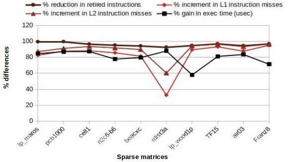
Table 2 presents the performance achieved by the SpMSpV codes generated by TACO, piecewise-regular, and SpComp for the sparse matrices and sparse vectors shown in Table 1. The performance is captured in terms of the number of retired instructions, % of retired instructions missed by L1 and L2 instruction caches, and execution time in micro-second (usec). We observe significant execution time improvement by SpComp compared to both TACO and Piecewise-regular framework. Although SpComp incurs a significant amount of relative instruction misses, the major saving happens due to the reduced number of retired instructions by the sparsity structure-specific execution of the SpComp-generated code.
The plot in Figure 9(a) illustrates the performance of SpComp compared to TACO. The % gain in execution time is inversely proportional to the % increment in L1 and L2 instruction misses but is limited to the % reduction of the retired instructions. The increments in relative instruction misses by L1 and L2 caches occur due to the presence of piecewise-regular loops. Note that, the % gain and % reduction by SpComp are computed as , where and denote the performance by TACO and SpComp respectively. Similarly, the % increment by SpComp is computed as .
 |
 |
| (a) | (b) |
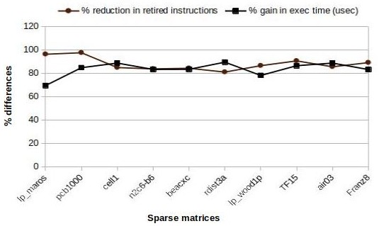
As illustrated in the plot in Figure 9(b), the % gain in execution time by SpComp compared to piecewise-regular framework is primarily dominated by the % reduction in retired instructions. This is quite obvious as, unlike the piecewise regular work, SpComp considers sparsity of both sparse matrix and sparse vector, making the code specific to both the sparsity structures. However, the increments in relative instruction miss by SpComp for lp_maros and pcb1000 occur due to the irregularity present in the SpMSpV output, resulting in piecewise-regular loops of small size. On the contrary, SpComp showcases significantly fewer relative instruction misses for rdist3a as the SpMSpV output showcases high regularity, resulting in large-sized loops.
5.2.2. Sparse Cholesky Decomposition
This matrix operation has utility in the circuit simulation domain, where the circuit is simulated until it converges. Here the sparsity structure models the physical connections of the circuit which remains unchanged throughout the simulation. In each iteration of the simulation the sparse matrix is factorized (Cholesky decomposed in the case of Hermitian positive-definite matrices) and the factorized matrix is used to solve the set of linear equations. In this reusable scenario, having a Cholesky decomposition customized to the underlying sparsity structure should benefit the overall application performance.
We consider the Cholesky decomposition , where is a factorization of Hermitian positive-definite matrix A into the product of a lower triangular matrix L and its conjugate transpose . The operation is mutable, i.e., alters the sparsity structure of the input by introducing fill-in elements, and has multiple statements and nested loops with loop-carried and inter-statement dependencies.
The SpComp-generated code is compared against CHOLMOD (Chen et al., 2008), the high-performance library for sparse Cholesky decomposition. CHOLMOD applies different ordering methods like Approximate Minimum Degree (AMD) (Amestoy et al., 2004), Column Approximate Minimum Degree(COLAMD) (Davis et al., 2004) etc. to reduce the fill-in of the factorized sparse matrix and selects the best-ordered matrix. However, we configure both CHOLMOD and SpComp to use only AMD permutation. CHOLMOD offers cholmod_analyze and cholmod_factorize routines to perform symbolic and numeric factorization respectively. We profile the cholmod_factorize function call for the evaluation.
We select the sparse matrices from the Suitesparse Matrix Collection (Davis, 2023a). As the Cholesky decomposition applies to symmetric positive definite matrices, it is challenging to identify such matrices from the collection. We have noticed that sparse matrices from the structural problem domain are primarily positive definite and thus can be Cholesky decomposed. In the collection, we have identified 200+ such Cholesky factorizable sparse matrices and selected 35+ matrices for our evaluation from the range of 1000 to 17000 numbers of nonzero elements. We see that a sparse matrix with more nonzeroes exhausts the available memory during code generation and thus is killed.
| Input sparse matrix | Output sparse matrix | Generated code | |||||
| Matrix | Size | Nonzeroes | Sparsity | Nonzeroes | fill-in | Amount of loop in | Avg loop |
| (%) | +fill-in | (%) | generated code(%) | size | |||
| nos1 | |||||||
| mesh3e1 | |||||||
| bcsstm11 | |||||||
| can_229 | |||||||
| bcsstm26 | |||||||
| mesh2e1 | |||||||
| bcsstk05 | |||||||
| lund_b | |||||||
| can_292 | |||||||
| dwt_193 | |||||||
| bcsstk04 | |||||||
| bcsstk19 | |||||||
| dwt_918 | |||||||
| dwt_1007 | |||||||
| dwt_1242 | |||||||
| bcsstm25 | |||||||
| dwt_992 | |||||||
Table 3 presents the sparsity structure of input and output sparse matrices and the structure of the generated piecewise regular loops for a few sparse matrices. All the matrices in the table have sparsity within the range of 79% to 99% and almost all of them introduce a considerable amount of fill-in when Cholesky decomposed. The amount of fill-in(%) is computed by , where and denote the number of non-zero elements before and after factorization. Sparse matrices bcsstm11, bcsstm26, and bcsstm25 are diagonal, and thus no fill-in element is generated when factorized. For these diagonal sparse matrices, SpComp generates a single regular loop with an average loop size of 1473, 1922, and 15439, the number of non-zero elements. In these cases, 100% of the generated code is looped back.
The rest of the sparse matrices in Table 3 showcase irregular sparsity structures and thus produce different amounts of fill-in elements and piecewise regular loops with different average loop sizes. As an instance, sparse matrix nos1 with 98.19% sparsity generates 7.03% fill-in elements when Cholesky decomposed and 37.72% of generated code is piecewise-regular loops with an average loop size of . Similarly, another irregular sparse matrix dwt_992 with 98.29% sparsity produces 56.59% fill-in elements and 95.95% of generated code represents piecewise-regular loops with an average loop size of 8.9.
| CHOLMOD | SpComp | |||||
|---|---|---|---|---|---|---|
| Matrix | Rtd | TLB | Exec | Rtd | TLB | Exec |
| instr | miss | time | instr | miss | time | |
| nos1 | 151641 | 151641 | 34 | 5312 | 12 | 7.9 |
| mesh3e1 | 425460 | 425460 | 108 | 61960 | 23 | 37 |
| bcsstm11 | 432790 | 432790 | 89 | 13458 | 13 | 6.8 |
| can_229 | 574458 | 574460 | 128 | 79141 | 26 | 42 |
| bcsstm26 | 561262 | 561262 | 113 | 17500 | 29 | 10 |
| mesh2e1 | 585133 | 585134 | 144 | 88186 | 27 | 47 |
| bcsstk05 | 492787 | 492788 | 106 | 82730 | 24 | 39 |
| lund_b | 498362 | 498363 | 103 | 80308 | 25 | 36 |
| can_292 | 474573 | 474574 | 111 | 59632 | 31 | 33 |
| dwt_193 | 1129067 | 1129068 | 217 | 378388 | 50 | 142 |
| bcsstk04 | 825630 | 825630 | 158 | 216535 | 38 | 87 |
| bcsstk19 | 1342154 | 1342158 | 344 | 118177 | 60 | 135 |
| dwt_918 | 2843603 | 2843604 | 791 | 763262 | 96 | 327 |
| dwt_1007 | 3593429 | 3593430 | 888 | 1007852 | 139 | 487 |
| dwt_1242 | 5139767 | 5139773 | 1364 | 1467372 | 165 | 596 |
| bcsstm25 | 4441657 | 4441681 | 1315 | 139182 | 83 | 81 |
| dwt_992 | 8419954 | 8419954 | 2123 | 2775950 | 276 | 1270 |
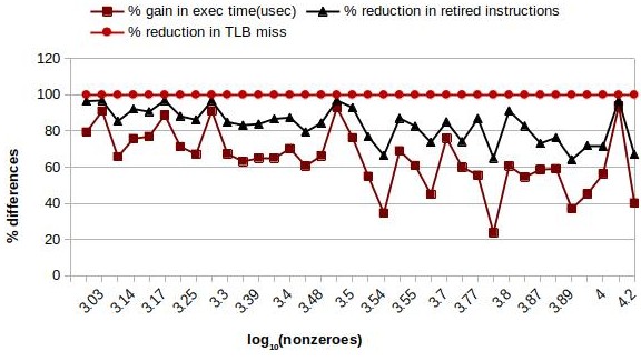 |
The graph in Figure 10 illustrates the performance gained by SpComp against CHOLMOD. The number of nonzero elements of sparse matrices is plotted against the logarithmic scale on X-axis. Considering the performance in terms of the number of retired instructions, the number of TLB miss, and execution time (usec) of CHOLMOD as the baseline, we plot the performance difference (in %) by SpComp against Y-axis. The performance difference is computed as , where and denote the performance by CHOLMOD and SpComp respectively.
We see a directly proportional relation between % gain in execution time and % reduction in the number of retired instructions. SpComp contributes to a lesser number of instructions and thus improves the execution time. We find 100% reduction in the instructions executed for use cases where the sparse matrices are diagonal, like bcsstm25 and bcsstm39. Additionally, we see 100% improvement in TLB misses for all the selected use cases. This happens due to the static allocation of the fill-in elements that avert the need for dynamic modification of sparse data storage, thus improving the TLB miss. Table 4 presents the raw performance numbers for the sparse matrices. We see an equal number of retired instructions and TLB misses by CHOLMOD, which implies dynamic memory allocation for all the nonzero elements including fill-in elements.
SpComp takes 4sec to perform the analysis on sparse matrix nos1 and 20min to perform the same on sparse matrix dwt_992. As expected, our approach generates large codes even for moderate-sized sparse matrices. In the case of dwt_992 with size and NNZ of 16744 the generated code size is 6.3 MB.
6. Related Work
Here we provide an overview of the work related to optimizing sparse matrix operations either by reorganizing data or by reorganizing computation. Over decades researchers have explored various optimization approaches and have established various techniques, either hand-crafted or compiler-aided.
Researchers have developed various hand-crafted algorithms involving custom data structures like CSR, CSC, COO, CDS, etc., (Eijkhout, 1992; Saad, 1994) that contain the data indices and values of the non-zero data elements. Hand-crafted libraries like Cholmod (Chen et al., 2008), Klu (Davis and Palamadai Natarajan, 2010), CSparse (Davis, 2006) etc. from SuiteSparse (Davis, 2023b); C++ supported SparseLib++ (Pozo et al., 2023; Dongarra et al., 1997), Eigen (Guennebaud et al., 2023); Python supported Numpy (num, 2015); Intel provided MKL (Intel, 2023), Radios (Schenk and Gärtner, 2004; Schenk et al., 2000); CUDA supported cuSparse (NVIDIA, 2023); Java supported Parallel Colt (Wendykier and Nagy, 2010); C, Fortran supported PaStiX (PaStiX, 2023; Hénon et al., 2002), MUMPS (Amestoy et al., 1998), SuperLU (Demmel et al., 1995) etc. are widely used in current practice. Although these libraries offer high-performing sparse matrix operations, they typically require human effort to build the libraries and port them to different architectures. Also, libraries are often difficult to be used in the application and composition of operations encapsulated within separate library functions may be challenging.
Compiler-aided optimization technique includes run-time optimization approaches like inspection-execution(Mirchandaney et al., 1988; Saltz and Mirchandaney, 1991; Ponnusamy et al., 1993) where the inspector profiles the memory access information, inspects data dependencies during execution, and uses this information to generate an optimized schedule. The executor executes the optimized schedule. Such optimization can be even hardware-aware like performing run-time optimization for distributed memory architecture (Mirchandaney et al., 1988; Baxter et al., 1989; Basumallik and Eigenmann, 2006), and shared memory architecture (Rauchwerger, 1998; Zhuang et al., 2009; Park et al., 2014; Norrish and Strout, 2015) etc. Compiler support has been developed to automatically reduce the time and space overhead of inspector-executor (Mohammadi et al., 2019, 2018; Venkat et al., 2015, 2016; Strout et al., 2018; Cheshmi et al., 2018; Ujaldon et al., 1995; Nandy et al., 2018). Polyhedral transformation mechanisms (Ravishankar et al., 2015; Venkat et al., 2014, 2015, 2016), Sparse Polyhedral Framework (SPF) (Strout et al., 2018, 2016) etc. address the cost reduction of the inspection. Other run-time approaches (Kamin et al., 2014; Ching-Hsien Hsu, 2002; Lee and Eigenmann, 2008; Ziantz et al., 1994; Li et al., 2015) propose optimal data distributions during execution such that both computation and communication overhead is reduced. Other run-time technique like Eggs (Tang et al., 2020) dynamically intercepts the arithmetic operations and performs symbolic execution by piggybacking onto Eigen code to accelerate the execution.
In contrast to run-time mechanisms, compile-time optimization techniques do not incur any execution-time overhead. Given the sparse input and code handling dense matrix operation, the work done by (Bik and Wijshoff, 1994a, b, 1996; Bik et al., 1998, 1994; Bik and Wijshoff, 1993) determine the best storage for sparse data and generate the code specific to the underlying storage but not specific to the sparsity structure of the input. They handle both single-statement and multi-statement loops and regular loop nests. The generated code contains indirect references. These approaches have been implemented in MT1 compiler (Bik et al., 1996), creating a sparse compiler to automatically convert a dense program into semantically equivalent sparse code. Given the best storage for the sparse data, (Kotlyar and Pingali, 1997; Stodghill, 1997; Kotlyar, 1999; Kotlyar et al., 1997a; Mateev et al., 2000; Kotlyar et al., 1997b) propose relational algebra-based techniques to generate efficient sparse matrix programs from dense matrix programs and specifications of the sparse input. Similar to (Bik and Wijshoff, 1994a, b, 1996; Bik et al., 1998, 1994), they do not handle mutable cases and generate code with indirect references. However, unlike the aforementioned work they handle arbitrary loop nests. Other compile-time techniques like Tensor Algebra Compiler(TACO) (Kjolstad et al., 2017; Kjolstad and Amarasinghe, 2023; Henry, 2020) automatically generate storage specific code for a given matrix operation. They provide a compiler-based technique to generate code for any combination of dense and sparse data. Bernoulli compiler proposes restructuring compiler to transform a sequential, dense matrix Conjugate-Gradient method into a parallel, sparse matrix program (K. et al., 1996).
Compared to immutable kernels, compile-time optimization of mutable kernels is intrinsically challenging due to the run-time generation of fill-in elements (George and Liu, 1975). Symbolic analysis (Davis et al., 2016) is a sparsity structure-specific graph technique to determine the computation pattern of any matrix operation. The information generated by the Symbolic analysis guides the optimization of the numeric computation. (Cheshmi et al., 2017, 2018, 2022) generate vectorized and task level parallel codes by decoupling symbolic analysis from the compile-time optimizations. The generated code is specific to the sparsity structure of the sparse matrices and is free of indirect references. However, the customization of the analysis to handle different kernels requires manual effort. (Pouchet and Rodríguez, 2018; Augustine et al., 2019) propose a fundamentally different approach where they construct polyhedra from the sparsity structure of the input matrix, and generate indirect reference free regular loops. The approach only applies to immutable kernels and the generated code supports out-of-order execution wherever applicable. Their work is the closest to our work available in the literature.
Alternate approaches include machine learning techniques and advanced search techniques to select the optimal storage format and suitable algorithms for different sparse matrix operations (Xie et al., 2019; Chen et al., 2019; Byun et al., 2012; Bik and Wijshoff, 1994b, 1996). Apart from generic run-time and compile-time optimization techniques, domain experts have also explored domain-specific sparse matrix optimization. As an instance, (Wu et al., 2011; Kapre and Dehon, 2009; Nechma and Zwolinski, 2015; Ge et al., 2017; Chen et al., 2012; Eljammaly et al., 2013; Hassan et al., 2015; Jheng et al., 2011; Fowers et al., 2014; Grigoras et al., 2015; Nurvitadhi et al., 2015) propose FPGA accelerated sparse matrix operations required in circuit simulation domain.
7. Conclusions and Future Work
SpComp is a fully automatic sparsity-structure specific compilation technique that uses data flow analysis to statically generate piecewise-regular codes customized to the underlying sparsity structures. The generated code is free of indirect access and is amenable to SIMD vectorization. It is valid until the sparsity structure changes.
We focus on the sparsity structure of the output matrices and not just that of the input matrices. The generality of our method arises from the fact that we drive our analysis by the sparsity structure of the output matrices which depend on the sparsity structure of the input matrices and hence is covered by the analysis. This generality arises from our use of abstract interpretation-based static analysis. Unlike the state-of-art methods, our method is fully automatic and does not require any manual effort to customize to different kernels.
In the future, we would like to parallelize our implementation which suffers from significant computation overhead and memory limitations while handling large matrices and computation-intensive kernels. We would also like to explore the possibility of using GPU-accelerated architectures for our implementation.
Currently, we generate SIMD parallelizable code specific to shared memory architectures. In the future, we would like to explore the generation of multiple programs multiple data (MPMD) parallelized codes specific to distributed architectures.
Finally, the current implementation considers the data index of each non-zero element individually. We would like to explore whether the polyhedra built from the sparsity structure of the input sparse matrices can be used to construct the precise sparsity structure of the output sparse matrices.
References
- (1)
- num (2015) 2015. Guide to NumPy 2nd. CreateSpace Independent Publishing Platform, USA. 364 pages.
- Amestoy et al. (1998) P.R. Amestoy, I.S. Duff, and J.-Y. L’Excellent. 1998. Multifrontal Parallel Distributed Symmetric and Unsymmetric Solvers. Comput. Methods Appl. Mech. Eng 184 (1998), 501–520.
- Amestoy et al. (2004) Patrick R. Amestoy, Timothy A. Davis, and Iain S. Duff. 2004. Algorithm 837: AMD, an Approximate Minimum Degree Ordering Algorithm. ACM Trans. Math. Softw. 30, 3 (Sept. 2004), 381–388. https://doi.org/10.1145/1024074.1024081
- Augustine et al. (2019) Travis Augustine, Janarthanan Sarma, Louis-Noël Pouchet, and Gabriel Rodríguez. June,2019. Generating piecewise-regular code from irregular structures. In Proceedings of the 40th ACM SIGPLAN Conference on Programming Language Design and Implementation (PLDI ’19). 625–639. https://doi.org/10.1145/3314221.3314615
- Banerjee (1988) Utpal K. Banerjee. 1988. Dependence Analysis for Supercomputing. Kluwer Academic Publishers, USA.
- Bastoul (2004) C. Bastoul. 2004. Code generation in the polyhedral model is easier than you think. In Proceedings. 13th International Conference on Parallel Architecture and Compilation Techniques, 2004. PACT 2004. 7–16. https://doi.org/10.1109/PACT.2004.1342537
- Bastoul et al. (2004) Cédric Bastoul, Albert Cohen, Sylvain Girbal, Saurabh Sharma, and Olivier Temam. 2004. Putting Polyhedral Loop Transformations to Work. In Languages and Compilers for Parallel Computing, Lawrence Rauchwerger (Ed.). Springer Berlin Heidelberg, Berlin, Heidelberg, 209–225.
- Basumallik and Eigenmann (2006) Ayon Basumallik and Rudolf Eigenmann. 2006. Optimizing Irregular Shared-Memory Applications for Distributed-Memory Systems. In Proceedings of the Eleventh ACM SIGPLAN Symposium on Principles and Practice of Parallel Programming (New York, New York, USA) (PPoPP ’06). Association for Computing Machinery, New York, NY, USA, 119–128. https://doi.org/10.1145/1122971.1122990
- Baxter et al. (1989) D. Baxter, R. Mirchandaney, and J. H. Saltz. 1989. Run-Time Parallelization and Scheduling of Loops. In Proceedings of the First Annual ACM Symposium on Parallel Algorithms and Architectures (Santa Fe, New Mexico, USA) (SPAA ’89). Association for Computing Machinery, New York, NY, USA, 303–312. https://doi.org/10.1145/72935.72967
- Benabderrahmane et al. (2010) Mohamed-Walid Benabderrahmane, Louis-Noël Pouchet, Albert Cohen, and Cédric Bastoul. 2010. The Polyhedral Model Is More Widely Applicable Than You Think. In Compiler Construction, Rajiv Gupta (Ed.). Springer Berlin Heidelberg, Berlin, Heidelberg, 283–303.
- Bik et al. (1996) Aart JC Bik, Peter JH Brinkhaus, and HAG Wijshoff. 1996. The Sparse Compiler MT1: A Reference Guide. Citeseer.
- Bik and Wijshoff (1993) Aart JC Bik and Harry AG Wijshoff. 1993. Compilation techniques for sparse matrix computations. In Proceedings of the 7th international conference on Supercomputing. 416–424.
- Bik et al. (1998) Aart J. C. Bik, Peter J. H. Brinkhaus, Peter M. W. Knijnenburg, and Harry A. G. Wijshoff. 1998. The Automatic Generation of Sparse Primitives. ACM Trans. Math. Softw. 24, 2 (June 1998), 190–225. https://doi.org/10.1145/290200.287636
- Bik et al. (1994) Aart J. C. Bik, Peter M. W. Knijenburg, and Harry A. G. Wijshoff. 1994. Reshaping Access Patterns for Generating Sparse Codes. In Proceedings of the 7th International Workshop on Languages and Compilers for Parallel Computing (LCPC ’94). Springer-Verlag, Berlin, Heidelberg, 406–420.
- Bik and Wijshoff (1994a) Aart J. C. Bik and Harry A. G. Wijshoff. 1994a. Nonzero Structure Analysis. In Proceedings of the 8th International Conference on Supercomputing (Manchester, England) (ICS ’94). Association for Computing Machinery, New York, NY, USA, 226–235. https://doi.org/10.1145/181181.181538
- Bik and Wijshoff (1996) A. J. C. Bik and H. A. G. Wijshoff. 1996. Automatic data structure selection and transformation for sparse matrix computations. IEEE Transactions on Parallel and Distributed Systems 7, 2 (Feb 1996), 109–126. https://doi.org/10.1109/71.485501
- Bik and Wijshoff (1994b) Aart J. C. Bik and Harry G. Wijshoff. 1994b. On automatic data structure selection and code generation for sparse computations. In Languages and Compilers for Parallel Computing, Utpal Banerjee, David Gelernter, Alex Nicolau, and David Padua (Eds.). Springer Berlin Heidelberg, Berlin, Heidelberg, 57–75.
- Byun et al. (2012) Jong-Ho Byun, Richard Y. Lin, Katherine A. Yelick, and James Demmel. 2012. Autotuning Sparse Matrix-Vector Multiplication for Multicore.
- Chen et al. (2019) Shizhao Chen, Jianbin Fang, Donglin Chen, Chuanfu Xu, and Zheng Wang. 2019. Optimizing Sparse Matrix-Vector Multiplication on Emerging Many-Core Architectures. arXiv:1805.11938 [cs.MS]
- Chen et al. (2012) X. Chen, Y. Wang, and H. Yang. 2012. An adaptive LU factorization algorithm for parallel circuit simulation. In 17th Asia and South Pacific Design Automation Conference. 359–364.
- Chen et al. (2008) Y. Chen, T. A. Davis, W. W. Hager, and S. Rajamanickam. 2008. Algorithm 887: CHOLMOD, Supernodal Sparse Cholesky Factorization and Update/Downdate. ACM Trans. Math. Software 35, 3 (2008), 1–14. http://dx.doi.org/10.1145/1391989.1391995
- Cheshmi et al. (2022) Kazem Cheshmi, Zachary Cetinic, and Maryam Mehri Dehnavi. 2022. Vectorizing sparse matrix computations with partially-strided codelets. In Proceedings of the International Conference on High Performance Computing, Networking, Storage and Analysis. 1–15.
- Cheshmi et al. (2017) Kazem Cheshmi, Shoaib Kamil, Michelle Strout, and MM Dehnavi. 2017. Sympiler: Transforming Sparse Matrix Codes by Decoupling Symbolic Analysis. (05 2017).
- Cheshmi et al. (2018) K. Cheshmi, S. Kamil, M. M. Strout, and M. M. Dehnavi. 2018. ParSy: Inspection and Transformation of Sparse Matrix Computations for Parallelism. In SC18: International Conference for High Performance Computing, Networking, Storage and Analysis. 779–793. https://doi.org/10.1109/SC.2018.00065
- Cheshmi et al. (2018) Kazem Cheshmi, Shoaib Kamil, Michelle Mills Strout, and Maryam Mehri Dehnavi. 2018. ParSy: Inspection and Transformation of Sparse Matrix Computations for Parallelism. In Proceedings of the International Conference for High Performance Computing, Networking, Storage, and Analysis (Dallas, Texas) (SC ’18). IEEE Press, Piscataway, NJ, USA, Article 62, 15 pages. https://doi.org/10.1109/SC.2018.00065
- Ching-Hsien Hsu (2002) Ching-Hsien Hsu. 2002. Optimization of sparse matrix redistribution on multicomputers. In Proceedings. International Conference on Parallel Processing Workshop. 615–622. https://doi.org/10.1109/ICPPW.2002.1039784
- Davis (2023a) Tim Davis. 2023a. SuiteSparse Matrix Collection. https://sparse.tamu.edu/.
- Davis (2006) Timothy A. Davis. 2006. Direct Methods for Sparse Linear Systems. Society for Industrial and Applied Mathematics, Philadelphia, PA, USA.
- Davis (2023b) Timothy A. Davis. 2023b. SuiteSparse : a suite of sparse matrix software. http://faculty.cse.tamu.edu/davis/suitesparse.html.
- Davis et al. (2004) Timothy A. Davis, John R. Gilbert, Stefan I. Larimore, and Esmond G. Ng. 2004. Algorithm 836: COLAMD, a Column Approximate Minimum Degree Ordering Algorithm. ACM Trans. Math. Softw. 30, 3 (Sept. 2004), 377–380. https://doi.org/10.1145/1024074.1024080
- Davis and Palamadai Natarajan (2010) T. A. Davis and E. Palamadai Natarajan. 2010. Algorithm 907: KLU, A Direct Sparse Solver for Circuit Simulation Problems. ACM Trans. Math. Software 37, 3 (Sept. 2010), 36:1–36:17. http://dx.doi.org/10.1145/1824801.1824814
- Davis et al. (2016) Timothy A. Davis, Sivasankaran Rajamanickam, and Wissam M. Sid-Lakhdar. 2016. A survey of direct methods for sparse linear systems. Acta Numerica 25 (2016), 383–566. https://doi.org/10.1017/S0962492916000076
- Demmel et al. (1995) James W. Demmel, Stanley C. Eisenstat, John R. Gilbert, Xiaoye S. Li, and Joseph W.H. Liu. 1995. A Supernodal Approach to Sparse Partial Pivoting. Technical Report. USA.
- Dongarra et al. (1997) Jack Dongarra, Andrew Lumsdaine, Xinhiu Niu, Roldan Pozo, and Karin Remington. 1997. A Sparse Matrix Library in C++ for High Performance Architectures. Proceedings of the Second Object Oriented Numerics Conference (05 1997).
- Eijkhout (1992) Victor Eijkhout. 1992. LAPACK Working Note 50: Distributed Sparse Data Structures for Linear Algebra Operations. Technical Report. Knoxville, TN, USA.
- Eljammaly et al. (2013) M. Eljammaly, Y. Hanafy, A. Wahdan, and A. Bayoumi. 2013. Hardware implementation of LU decomposition using dataflow architecture on FPGA. In 2013 5th International Conference on Computer Science and Information Technology. 298–302.
- Fowers et al. (2014) J. Fowers, K. Ovtcharov, K. Strauss, E. S. Chung, and G. Stitt. 2014. A High Memory Bandwidth FPGA Accelerator for Sparse Matrix-Vector Multiplication. In 2014 IEEE 22nd Annual International Symposium on Field-Programmable Custom Computing Machines. 36–43.
- Ge et al. (2017) X. Ge, H. Zhu, F. Yang, L. Wang, and X. Zeng. 2017. Parallel sparse LU decomposition using FPGA with an efficient cache architecture. In 2017 IEEE 12th International Conference on ASIC (ASICON). 259–262. https://doi.org/10.1109/ASICON.2017.8252462
- George and Liu (1975) Alan George and Wai-Hung Liu. 1975. A Note on Fill for Sparse Matrices. SIAM J. Numer. Anal. 12, 3 (1975), 452–455. http://www.jstor.org/stable/2156057
- Grigoras et al. (2015) P. Grigoras, P. Burovskiy, E. Hung, and W. Luk. 2015. Accelerating SpMV on FPGAs by Compressing Nonzero Values. In 2015 IEEE 23rd Annual International Symposium on Field-Programmable Custom Computing Machines. 64–67.
- Guennebaud et al. (2023) Gaël Guennebaud, Benoît Jacob, et al. 2023. Eigen v3. http://eigen.tuxfamily.org.
- Hassan et al. (2015) M. W. Hassan, A. E. Helal, and Y. Y. Hanafy. 2015. High Performance Sparse LU Solver FPGA Accelerator Using a Static Synchronous Data Flow Model. In 2015 IEEE 23rd Annual International Symposium on Field-Programmable Custom Computing Machines. 29–29.
- Henry (2020) Rawn Tristan Henry. 2020. A framework for computing on sparse tensors based on operator properties. Ph. D. Dissertation. USA.
- Hénon et al. (2002) Pascal Hénon, Pierre Ramet, and Jean Roman. 2002. PaStiX: A High-Performance Parallel Direct Solver for Sparse Symmetric Definite Systems. Parallel Comput. 28 (02 2002), 301–321. https://doi.org/10.1016/S0167-8191(01)00141-7
- Intel (2023) Intel. 2023. Intel Math Kernel Library. https://software.intel.com/en-us/mkl.
- Jheng et al. (2011) H. Y. Jheng, C. C. Sun, S. J. Ruan, and J. Goetze. 2011. FPGA acceleration of Sparse Matrix-Vector Multiplication based on Network-on-Chip. In 2011 19th European Signal Processing Conference. 744–748.
- K. et al. (1996) Vladimir K., Keshav P., and Paul S. 1996. Automatic parallelization of the conjugate gradient algorithm. In Languages and Compilers for Parallel Computing. Springer Berlin Heidelberg, Berlin, Heidelberg, 480–499.
- Kamin et al. (2014) Sam Kamin, María Jesús Garzarán, Barış Aktemur, Danqing Xu, Buse Yılmaz, and Zhongbo Chen. 2014. Optimization by Runtime Specialization for Sparse Matrix-vector Multiplication. SIGPLAN Not. 50, 3 (Sept. 2014), 93–102. https://doi.org/10.1145/2775053.2658773
- Kapre and Dehon (2009) Nachiket Kapre and Andre Dehon. 2009. Parallelizing sparse Matrix Solve for SPICE circuit simulation using FPGAs. In In: Proc. Field-Programmable Technology. 190–198.
- Kennedy and Allen (2001) Ken Kennedy and John R. Allen. 2001. Optimizing Compilers for Modern Architectures: A Dependence-Based Approach. Morgan Kaufmann Publishers Inc., San Francisco, CA, USA.
- Kjolstad and Amarasinghe (2023) Fredrik Kjolstad and Saman Amarasinghe. 2023. TACO: The Tensor Algebra Compiler. http://tensor-compiler.org/.
- Kjolstad et al. (2017) Fredrik Kjolstad, Stephen Chou, David Lugato, Shoaib Kamil, and Saman Amarasinghe. 2017. Taco: A tool to generate tensor algebra kernels. In 2017 32nd IEEE/ACM International Conference on Automated Software Engineering (ASE). 943–948. https://doi.org/10.1109/ASE.2017.8115709
- Kotlyar (1999) Vladimir Kotlyar. 1999. Relational Algebraic Techniques for the Synthesis of Sparse Matrix Programs. Ph. D. Dissertation. USA. Advisor(s) Pingali, Keshav. AAI9910244.
- Kotlyar and Pingali (1997) Vladimir Kotlyar and Keshav Pingali. 1997. Sparse Code Generation for Imperfectly Nested Loops with Dependences. In Proceedings of the 11th International Conference on Supercomputing (Vienna, Austria) (ICS ’97). Association for Computing Machinery, New York, NY, USA, 188–195. https://doi.org/10.1145/263580.263630
- Kotlyar et al. (1997a) Vladimir Kotlyar, Keshav Pingali, and Paul Stodghill. 1997a. Compiling Parallel Code for Sparse Matrix Applications. In Proceedings of the 1997 ACM/IEEE Conference on Supercomputing (San Jose, CA) (SC ’97). Association for Computing Machinery, New York, NY, USA, 1–18. https://doi.org/10.1145/509593.509603
- Kotlyar et al. (1997b) Vladimir Kotlyar, Keshav Pingali, and Paul Stodghill. 1997b. A Relational Approach to the Compilation of Sparse Matrix Programs. Technical Report. USA.
- Lee and Eigenmann (2008) Seyong Lee and Rudolf Eigenmann. 2008. Adaptive Runtime Tuning of Parallel Sparse Matrix-vector Multiplication on Distributed Memory Systems. In Proceedings of the 22Nd Annual International Conference on Supercomputing (Island of Kos, Greece) (ICS ’08). ACM, New York, NY, USA, 195–204. https://doi.org/10.1145/1375527.1375558
- Li et al. (2015) ShiGang Li, ChangJun Hu, JunChao Zhang, and YunQuan Zhang. 2015. Automatic tuning of sparse matrix-vector multiplication on multicore clusters. Science China Information Sciences 58, 9 (01 Sep 2015), 1–14. https://doi.org/10.1007/s11432-014-5254-x
- Mateev et al. (2000) Nikolay Mateev, Keshav Pingali, Paul Stodghill, and Vladimir Kotlyar. 2000. Next-Generation Generic Programming and Its Application to Sparse Matrix Computations. In Proceedings of the 14th International Conference on Supercomputing (Santa Fe, New Mexico, USA) (ICS ’00). Association for Computing Machinery, New York, NY, USA, 88–99. https://doi.org/10.1145/335231.335240
- Mirchandaney et al. (1988) R. Mirchandaney, J. Saltz, R.M. Smith, D.M. Nicol, and Kay Crowley. 1988. Principles of run-time support for parallel processors. Proceedings of the 1988 ACM International Conference on Supercomputing (July 1988), 140–152.
- Mohammadi et al. (2018) Mahdi Soltan Mohammadi, Kazem Cheshmi, Ganesh Gopalakrishnan, Mary W. Hall, Maryam Mehri Dehnavi, Anand Venkat, Tomofumi Yuki, and Michelle Mills Strout. 2018. Sparse Matrix Code Dependence Analysis Simplification at Compile Time. CoRR abs/1807.10852 (2018). arXiv:1807.10852 http://arxiv.org/abs/1807.10852
- Mohammadi et al. (2019) Mahdi Soltan Mohammadi, Tomofumi Yuki, Kazem Cheshmi, Eddie C. Davis, Mary Hall, Maryam Mehri Dehnavi, Payal Nandy, Catherine Olschanowsky, Anand Venkat, and Michelle Mills Strout. 2019. Sparse Computation Data Dependence Simplification for Efficient Compiler-generated Inspectors. In Proceedings of the 40th ACM SIGPLAN Conference on Programming Language Design and Implementation (Phoenix, AZ, USA) (PLDI 2019). ACM, New York, NY, USA, 594–609. https://doi.org/10.1145/3314221.3314646
- Møller and Schwartzbach (2015) Andres Møller and Michael I. Schwartzbach. 2015. Static Program Analysis. Department of Computer Science, Aarhus University.
- Nandy et al. (2018) Payal Nandy, Eddie C. Davis, and Mahdi Soltan Mohammadi. 2018. Abstractions for specifying sparse matrix data transformations. In Proc. 8th Int. Workshop Polyhedral Compilation Techn. (IMPACT). 1–10.
- Nechma and Zwolinski (2015) T. Nechma and M. Zwolinski. 2015. Parallel Sparse Matrix Solution for Circuit Simulation on FPGAs. IEEE Trans. Comput. 64, 4 (2015), 1090–1103.
- Norrish and Strout (2015) Michael Norrish and Michelle Mills Strout. 2015. An Approach for Proving the Correctness of Inspector/Executor Transformations. In Languages and Compilers for Parallel Computing, James Brodman and Peng Tu (Eds.). Springer International Publishing, Cham, 131–145.
- Nurvitadhi et al. (2015) E. Nurvitadhi, A. Mishra, and D. Marr. 2015. A sparse matrix vector multiply accelerator for support vector machine. In 2015 International Conference on Compilers, Architecture and Synthesis for Embedded Systems (CASES). 109–116.
- NVIDIA (2023) NVIDIA. 2023. CUSPARSE. https://developer.nvidia.com/cusparse.
- Park et al. (2014) Jongsoo Park, Mikhail Smelyanskiy, Narayanan Sundaram, and Pradeep Dubey. 2014. Sparsifying Synchronization for High-Performance Shared-Memory Sparse Triangular Solver. In Supercomputing, Julian Martin Kunkel, Thomas Ludwig, and Hans Werner Meuer (Eds.). Springer International Publishing, Cham, 124–140.
- PaStiX (2023) PaStiX. 2023. PaStiX. http://pastix.gforge.inria.fr/files/README-txt.html.
- Ponnusamy et al. (1993) R. Ponnusamy, J. Saltz, and A. Choudhary. 1993. Runtime Compilation Techniques for Data Partitioning and Communication Schedule Reuse. In Proceedings of the 1993 ACM/IEEE Conference on Supercomputing (Portland, Oregon, USA) (Supercomputing ’93). Association for Computing Machinery, New York, NY, USA, 361–370. https://doi.org/10.1145/169627.169752
- Pouchet and Rodríguez (2018) Louis-Noël Pouchet and Gabriel Rodríguez. 2018. Polyhedral modeling of immutable sparse matrices. (2018).
- Pozo et al. (2023) Roldan Pozo, Karin Remington, and Andrew Lumsdaine. 2023. SparseLib++ Sparse Matrix Class Library. https://math.nist.gov/sparselib++/.
- Rauchwerger (1998) Lawrence Rauchwerger. 1998. Run-time parallelization: Its time has come. Parallel Comput. 24, 3 (1998), 527–556. https://doi.org/10.1016/S0167-8191(98)00024-6
- Ravishankar et al. (2015) Mahesh Ravishankar, Roshan Dathathri, Venmugil Elango, Louis-Noël Pouchet, J. Ramanujam, Atanas Rountev, and P. Sadayappan. 2015. Distributed Memory Code Generation for Mixed Irregular/Regular Computations. In Proceedings of the 20th ACM SIGPLAN Symposium on Principles and Practice of Parallel Programming (San Francisco, CA, USA) (PPoPP 2015). Association for Computing Machinery, New York, NY, USA, 65–75. https://doi.org/10.1145/2688500.2688515
- Rodríguez (2022) Gabriel Rodríguez. 2022. poly-spmv. https://gitlab.com/grodriguez.udc/poly-spmv.
- Saad (1994) Youcef Saad. 1994. SPARSKIT: a basic tool kit for sparse matrix computations - Version 2.
- Saltz and Mirchandaney (1991) J. Saltz and R. Mirchandaney. 1991. The preprocessed doacross loop. Proceedings of the Int. Conf. Parallel Process(ICPP) 2 (August 1991), 174–179.
- Schenk and Gärtner (2004) Olaf Schenk and Klaus Gärtner. 2004. Solving Unsymmetric Sparse Systems of Linear Equations with PARDISO. Future Gener. Comput. Syst. 20, 3 (April 2004), 475–487. https://doi.org/10.1016/j.future.2003.07.011
- Schenk et al. (2000) O. Schenk, K. Gärtner, and W. Fichtner. 2000. Efficient Sparse LU Factorization with Left-Right Looking Strategy on Shared Memory Multiprocessors. BIT Numerical Mathematics 40 (2000), 158–176.
- Stodghill (1997) Paul Vinson Stodghill. 1997. A Relational Approach to the Automatic Generation of Sequential Sparse Matrix Codes. Ph. D. Dissertation. USA.
- Strout et al. (2018) M. M. Strout, M. Hall, and C. Olschanowsky. 2018. The Sparse Polyhedral Framework: Composing Compiler-Generated Inspector-Executor Code. Proc. IEEE 106 (Nov 2018), 1921–1934. https://doi.org/10.1109/JPROC.2018.2857721
- Strout et al. (2016) Michelle Mills Strout, Alan LaMielle, Larry Carter, Jeanne Ferrante, Barbara Kreaseck, and Catherine Olschanowsky. 2016. An approach for code generation in the Sparse Polyhedral Framework. Parallel Comput. 53 (2016), 32–57. https://doi.org/10.1016/j.parco.2016.02.004
- Tang et al. (2020) Xuan Tang, Teseo Schneider, Shoaib Kamil, Aurojit Panda, Jinyang Li, and Daniele Panozzo. 2020. EGGS: Sparsity‐Specific Code Generation. Computer Graphics Forum 39 (08 2020), 209–219. https://doi.org/10.1111/cgf.14080
- Terpstra et al. (2022) Dan Terpstra, Heike Jagode, Haihang You, and Jack Dongarra. 2022. Collecting Performance Data with PAPI-C. https://icl.utk.edu/papi/.
- Ujaldon et al. (1995) M. Ujaldon, S. D. Sharma, J. Saltz, and E. L. Zapata. 1995. Run-time techniques for parallelizing sparse matrix problems. In Parallel Algorithms for Irregularly Structured Problems, Afonso Ferreira and José Rolim (Eds.). Springer Berlin Heidelberg, Berlin, Heidelberg, 43–57.
- Venkat et al. (2015) Anand Venkat, Mary Hall, and Michelle Strout. 2015. Loop and Data Transformations for Sparse Matrix Code. In Proceedings of the 36th ACM SIGPLAN Conference on Programming Language Design and Implementation (Portland, OR, USA) (PLDI ’15). ACM, New York, NY, USA, 521–532. https://doi.org/10.1145/2737924.2738003
- Venkat et al. (2016) Anand Venkat, Mahdi Soltan Mohammadi, Jongsoo Park, Hongbo Rong, Rajkishore Barik, Michelle Mills Strout, and Mary Hall. 2016. Automating Wavefront Parallelization for Sparse Matrix Computations. In Proceedings of the International Conference for High Performance Computing, Networking, Storage and Analysis (Salt Lake City, Utah) (SC ’16). IEEE Press, Piscataway, NJ, USA, Article 41, 12 pages. http://dl.acm.org/citation.cfm?id=3014904.3014959
- Venkat et al. (2014) Anand Venkat, Manu Shantharam, Mary Hall, and Michelle Mills Strout. 2014. Non-Affine Extensions to Polyhedral Code Generation. In Proceedings of Annual IEEE/ACM International Symposium on Code Generation and Optimization (Orlando, FL, USA) (CGO ’14). Association for Computing Machinery, New York, NY, USA, 185–194. https://doi.org/10.1145/2581122.2544141
- Wendykier and Nagy (2010) Piotr Wendykier and James G. Nagy. 2010. Parallel Colt: A High-Performance Java Library for Scientific Computing and Image Processing. TOMS 37 (September 2010). https://doi.org/10.1145/1824801.1824809
- Wu et al. (2011) Wei Wu, Yi Shan, Xiaoming Chen, Yu Wang, and Huazhong Yang. 2011. FPGA Accelerated Parallel Sparse Matrix Factorization for Circuit Simulations. In Reconfigurable Computing: Architectures, Tools and Applications, Andreas Koch, Ram Krishnamurthy, John McAllister, Roger Woods, and Tarek El-Ghazawi (Eds.). Springer Berlin Heidelberg, Berlin, Heidelberg, 302–315.
- Xie et al. (2019) Zhen Xie, Guangming Tan, Weifeng Liu, and Ninghui Sun. 2019. IA-SpGEMM: An Input-aware Auto-tuning Framework for Parallel Sparse Matrix-matrix Multiplication. In Proceedings of the ACM International Conference on Supercomputing (Phoenix, Arizona) (ICS ’19). ACM, New York, NY, USA, 94–105. https://doi.org/10.1145/3330345.3330354
- Zhuang et al. (2009) X. Zhuang, A. E. Eichenberger, Y. Luo, K. O’Brien, and K. O’Brien. 2009. Exploiting Parallelism with Dependence-Aware Scheduling. In 2009 18th International Conference on Parallel Architectures and Compilation Techniques. 193–202. https://doi.org/10.1109/PACT.2009.10
- Ziantz et al. (1994) Louis H. Ziantz, Can C. Özturan, and Boleslaw K. Szymanski. 1994. Run-time optimization of sparse matrix-vector multiplication on SIMD machines. In PARLE’94 Parallel Architectures and Languages Europe, Costas Halatsis, Dimitrios Maritsas, George Philokyprou, and Sergios Theodoridis (Eds.). Springer Berlin Heidelberg, Berlin, Heidelberg, 313–322.