Spectral
enclosures for non-self-adjoint extensions of symmetric operators
Jussi Behrndt
Technische Universität Graz,
Institut für Angewandte Mathematik,
Steyrergasse 30,
8010 Graz, Austria
behrndt@tugraz.at, Matthias Langer
Department of Mathematics and Statistics,
University of Strathclyde,
26 Richmond Street, Glasgow G1 1XH, United Kingdom
m.langer@strath.ac.uk, Vladimir Lotoreichik
Department of Theoretical Physics, Nuclear Physics Institute CAS,
250 68 Řež near Prague, Czech Republic
lotoreichik@ujf.cas.cz and Jonathan Rohleder
Stockholms universitet, Matematiska institutionen, 10691 Stockholm, Sweden
jonathan.rohleder@math.su.se
Abstract.
The spectral properties of non-self-adjoint extensions of a symmetric operator
in a Hilbert space are studied with the help of ordinary and quasi boundary triples
and the corresponding Weyl functions. These extensions are given in terms of
abstract boundary conditions involving an (in general non-symmetric) boundary operator .
In the abstract part of this paper, sufficient conditions for sectoriality
and m-sectoriality as well as sufficient conditions for to have a non-empty
resolvent set are provided in terms of the parameter and the Weyl function.
Special attention is paid to Weyl functions that decay along the negative real line
or inside some sector in the complex plane, and spectral enclosures for
are proved in this situation.
The abstract results are applied to elliptic differential operators with
local and non-local Robin boundary conditions on unbounded domains,
to Schrödinger operators with -potentials of complex strengths
supported on unbounded hypersurfaces or infinitely many points on the real line,
and to quantum graphs with non-self-adjoint vertex couplings.
Keywords: non-self-adjoint extension, spectral enclosure,
differential operator, Weyl function.
Mathematics Subject Classification (MSC2010): 47A10;
35P05, 35J25, 81Q12, 35J10, 34L40, 81Q35.
Spectral problems for differential operators in Hilbert spaces and related
boundary value problems have attracted a lot of attention in the last decades
and have strongly influenced the development of modern functional analysis and operator theory.
For example, the classical treatment of Sturm–Liouville operators
and the corresponding Titchmarsh–Weyl theory in Hilbert spaces have led
to the abstract concept of boundary triples and their Weyl functions (see [43, 55, 82, 96]),
which is an efficient and well-established tool to investigate closed extensions
of symmetric operators and their spectral properties via abstract boundary maps and an
analytic function; see, e.g. [1, 5, 40, 41, 42, 44, 53, 56, 115, 117, 125].
The more recent notion of quasi boundary triples and their Weyl functions are
inspired by PDE analysis in a similar way. This abstract concept from [22, 24]
is tailor-made for spectral problems involving elliptic partial differential operators
and the corresponding boundary value problems; the Weyl function of a quasi boundary triple
is the abstract counterpart of the Dirichlet-to-Neumann map.
For different abstract treatments of elliptic PDEs and Dirichlet-to-Neumann maps
we refer to the classical works [84, 128] and the more recent approaches
[11, 12, 13, 30, 54, 77, 78, 79, 80, 83, 91, 118, 122, 124].
To recall the notions of ordinary and quasi boundary triples in more detail,
let be a densely defined, closed, symmetric operator in a
Hilbert space and let denote its adjoint;
then is said to be an ordinary boundary triple
for if are linear mappings from
the domain of into an auxiliary Hilbert space
that satisfy the abstract Lagrange or Green identity
(1.1)
and a certain maximality condition. The corresponding Weyl function
is an operator-valued function in , which is defined by
(1.2)
where is a self-adjoint operator in .
For a singular Sturm–Liouville expression in
with a real-valued potential the operators and
can be chosen as the minimal and maximal operators, respectively, together
with and , for ;
in this case the corresponding abstract Weyl function coincides with the
classical Titchmarsh–Weyl -function.
The notion of quasi boundary triples is a natural generalization of the
concept above, inspired by, and developed for, the treatment of elliptic differential operators.
The main difference is, that the boundary maps and are
only defined on a subspace of , where is an operator
in which satisfies .
The identities (1.1) and (1.2) are only required to hold
for elements in ; see Section 2 for precise definitions.
For the Schrödinger operator in
with a real-valued potential
on a domain with a sufficiently regular boundary ,
the operators and
can again be taken as the minimal and maximal operator, respectively, and a
convenient choice for the domain of is .
Then and
,
(where the latter denote the normal derivative and trace)
form a quasi boundary triple, and the corresponding Weyl function
is the energy-dependent Neumann-to-Dirichlet map.
The main focus of this paper is on non-self-adjoint extensions of that are
restrictions of parameterized by an ordinary or quasi boundary triple and
an (in general non-self-adjoint) boundary parameter, and to describe
their spectral properties.
For a quasi boundary triple and a linear operator
in we consider the operator
(1.3)
in . The principal results of this paper include (a) a sufficient condition
for to be m-sectorial and (b) enclosures for the numerical range
and the spectrum of the operator in parabola-type regions.
The latter make use of decay properties of the Weyl function
along the negative half-axis or inside sectors in the complex plane;
in order to make these results easily applicable, we provide (c) an abstract
sufficient condition for the Weyl function to decay appropriately.
We point out that, to the best of our knowledge, these results are also new in
the special case of ordinary boundary triples.
While the operator can be regarded as a perturbation of
the self-adjoint operator in the resolvent sense, let us mention
that the spectra of additive non-self-adjoint perturbations of
self-adjoint operators were studied recently in, e.g. [48, 49, 50, 51, 71].
In the second half of the present paper, we provide applications of
these results to several classes of operators, namely to elliptic differential operators
with local and non-local Robin boundary conditions on domains with
possibly non-compact boundaries, to Schrödinger operators with -interactions
of complex strength supported on hypersurfaces, to infinitely many point -interactions
on the real line, and to quantum graphs with non-self-adjoint vertex couplings.
Let us explain in more detail the structure, methodology, and results of this paper.
After the preliminary Section 2, our first main result is
Theorem 3.1, where it is shown that, under certain assumptions on the
Weyl function and the boundary parameter , the operator in (1.3) is sectorial,
and a sector containing the numerical range of is specified.
However, in applications it is essential to ensure that a sectorial
operator is m-sectorial; hence the next main objective is to prove that the resolvent set
of the operator in (1.3) is non-empty, which is a non-trivial
question particularly for quasi boundary triples.
This problem is treated in Section 4.
The principal result here is Theorem 4.1,
in which we provide sufficient conditions for
in terms of the operator and the parameter .
In this context also a Krein-type resolvent formula is obtained, and the adjoint of
is related to a dual parameter ; cf. [27, 29]
for the special case of symmetric . We list various corollaries of
Theorem 4.1 for more specialized situations.
We point out that an alternative description of sectorial and m-sectorial extensions
of a symmetric operator can be found in [14, 114]; see also the review article [15]
and [16, 17, 18].
Section 4 is complemented by two propositions
on Schatten–von Neumann properties for the resolvent difference of and ;
cf. [27, 55] for related abstract results and,
e.g. [21, 26, 33, 85, 112, 115] for applications to differential operators.
Such estimates can be used, for instance, to get bounds on the discrete spectrum of ;
cf. [51].
In Section 5 we consider the situation when the
Weyl function converges to in norm along the negative half-axis
or in some sector in the complex plane.
The most important result in this section is Theorem 5.6
where, under the assumption that decays like a power of ,
the numerical range and the spectrum of are contained in a parabola-type region.
Spectral enclosures of this type with more restrictive assumptions on were obtained
for elliptic partial differential operators in [19, 20, 73];
similar enclosures for Schrödinger operators with complex-valued regular
potentials can be found in [2, 71, 108].
They also appear in the abstract settings of so-called -subordinate perturbations [131].
Finally, as the last topic within the abstract part of this paper,
we prove in Theorem 6.1 that the Weyl function decays
along the negative real line or in suitable complex sectors with a certain
rate if the map is bounded
for some and some ,
where the rate of the decay depends on . Example 6.4
shows the sharpness of this result.
Our abstract results are applied in Section 7 to elliptic
partial differential operators with (in general non-local) Robin boundary conditions
on domains with possibly non-compact boundaries; the class of admissible unbounded domains includes,
for instance, domains of waveguide-type as considered in [34, 67].
In Section 8 we apply our abstract results to Schrödinger operators
in with -potentials of complex strength supported on
(not necessarily bounded) hypersurfaces. We indicate also how our abstract methods
can be combined with very recent norm estimates from [75] in order to
obtain further spectral enclosures and to establish absence of non-real spectrum
for ‘weak’ complex -interactions in space dimensions for compact hypersurfaces.
Finally, we apply our machinery to Schrödinger operators on the real line
with non-Hermitian -interactions supported on infinitely many points
in Section 9, and to Laplacians on finite
(not necessarily compact) graphs with non-self-adjoint vertex couplings
in Section 10.
Each of these sections has the same structure: after the problem under
consideration is explained, first a quasi (or ordinary) boundary triple
and its Weyl function are provided; next a lemma on the decay of the Weyl
function is proved, and then a main result on spectral properties and enclosures
is formulated, which can be derived easily from that decay together with
the abstract results in the first part of this paper in each particular situation.
To illustrate the different types of boundary conditions and interactions,
more specialized cases and explicit examples are included in
Sections 7–10.
Finally, let us fix some notation. By we denote the branch
of the complex square root such that
for all .
Let us set and
.
Moreover, for any bounded, complex-valued function we use
the abbreviation .
The space of bounded, everywhere defined operators from a
Hilbert space to another Hilbert space
is denoted by ,
and we set .
The Schatten–von Neumann ideal that consists of all compact operators from
to whose singular values are -summable is denoted by ,
and we set ;
see, e.g. [81] for a detailed study of the -classes.
Furthermore, for each densely defined operator in a Hilbert space
we write and
for its real and imaginary part, respectively, and,
if is closed, we denote by and its
resolvent set and spectrum, respectively.
2. Quasi boundary triples and their Weyl functions
In this preparatory section we first recall the notion and some properties of
quasi boundary triples and their Weyl functions from [22, 24].
Moreover, we discuss some elementary estimates and decay properties of the Weyl function.
In the following let be a densely defined, closed, symmetric operator
in a Hilbert space .
Definition 2.1.
Let be a linear operator in such that .
A triple is called a quasi boundary triple
for if is a Hilbert space and
are linear mappings such that
(i)
the abstract Green identity
(2.1)
holds for all ,
where denotes the inner product both in and ;
(ii)
the map has dense range;
(iii)
is a self-adjoint operator in .
If condition (ii) is replaced by the condition
(ii)’
the map is onto,
then is called a generalized boundary triple
for .
The notion of quasi boundary triples was introduced in [22, Definition 2.1].
The concept of generalized boundary triples appeared first
in [56, Definition 6.1]. It follows from [56, Lemma 6.1]
that each generalized boundary triple is also a quasi boundary triple.
We remark that the converse is in general not true.
A quasi or generalized boundary triple reduces to an ordinary boundary triple
if the map in condition (ii) is onto (see [22, Corollary 3.2]).
In this case is closed and coincides with ,
and in condition (iii) is automatically self-adjoint. For the
convenience of the reader we recall the usual definition of ordinary boundary triples.
Definition 2.2.
A triple is called an ordinary boundary triple
for if is a Hilbert space and
are linear mappings such that
(i)
the abstract Green identity
(2.2)
holds for all ;
(ii)
the map is onto.
We refer the reader to [22, 24] for a detailed study of quasi boundary triples,
to [52, 56] for generalized boundary triples
and to [43, 44, 55, 82, 96] for ordinary boundary triples.
For later purposes we recall the following result,
which is useful to determine the adjoint and a (quasi) boundary triple
for a given symmetric operator; see [22, Theorem 2.3].
Theorem 2.3.
Let and be Hilbert spaces and let be a linear operator in .
Assume that are linear mappings such
that the following conditions hold:
(i)
the abstract Green identity
holds for all ;
(ii)
the map
has dense range and is dense in ;
(iii)
is an extension of a self-adjoint
operator .
Then the restriction
is a densely defined closed symmetric operator in ,
, and
is a quasi boundary triple for with .
If, in addition, the operator is closed or, equivalently, the map
is onto,
then and is an ordinary boundary triple
for with .
In the following let be a quasi boundary triple
for . Since is self-adjoint,
we have , and
for each the direct sum decomposition
holds. In particular, the restriction of the map to
is injective. This allows the following definition.
Definition 2.4.
The -field and the Weyl function corresponding to the
quasi boundary triple are defined by
and
respectively.
The values of the -field are operators defined
on the dense subspace which map
onto . The values of the Weyl function
are densely defined operators in mapping into .
In particular, if is a generalized
or ordinary boundary triple, then and
are defined on , and it can be shown
that and
in this case.
Next we list some important properties of the -field and the
Weyl function corresponding to a quasi boundary triple ,
which can be found in [22, Proposition 2.6] or [24, Propositions 6.13 and 6.14].
These properties are well known for the -field and Weyl function
corresponding to a generalized or ordinary boundary triple.
Let . Then the adjoint operator
is bounded and satisfies
(2.3)
hence also is bounded and
.
One has the useful identity
(2.4)
for , which implies
(2.5)
With the help of the functional calculus of the self-adjoint operator
one can conclude from (2.5) that
(2.6)
The values of the Weyl function satisfy
and,
in particular, the operators are closable.
In general, the operators and their closures
are not bounded.
However, if is bounded for some ,
then is bounded for all ; see Lemma 2.5 below.
The function is holomorphic in the sense that
for any fixed it can be written as the sum of the possibly
unbounded operator and a -valued holomorphic function,
for all . In particular, is a bounded operator
for each .
Further, for every we have
for all and all , and hence the th strong
derivative (viewed as an operator defined on )
admits a continuous extension .
It satisfies
The Weyl function also satisfies (see [22, Proposition 2.6 (v)])
(2.8)
and with and the
relation it follows that
(2.9)
In the case when the values of are bounded operators we provide
a simple bound for the norms
in the next lemma.
Lemma 2.5.
Let be a quasi boundary triple for
with corresponding Weyl function . Assume that is bounded
for one .
Then is bounded for all , and the estimate
(2.10)
holds for all .
Proof.
It follows from (2.8), the relation
and (2.3)
that is bounded for all if it is bounded for one .
Moreover, from the second identity in (2.9) we conclude that
(2.11)
where we have used that .
If we replace on the right-hand side of (2.8)
with the right-hand side of (2.4), we obtain the representation
(2.12)
By combining (2.11) and (2.12), for
we obtain the estimate
Decay properties of the Weyl function play an important role in this paper.
The next lemma shows that a decay of the Weyl function along a non-real ray
implies a uniform decay in certain sectors.
Lemma 2.6.
Let be a quasi boundary triple for
with corresponding Weyl function . Assume that is bounded
for one (and hence for all)
and fix .
Then for every interval
or one has
which shows (2.13)
since the expression in the brackets on the right-hand side of (2.14)
is uniformly bounded in .
∎
In the context of the previous lemma we remark that
decays at
most as
since grows at most linearly
as it is a Nevanlinna function for every .
We also recall from [29, Lemma 2.3] that for
the function
is strictly increasing on each interval in ; moreover, if
is bounded from below and
for all , then
(2.15)
In the next proposition the case when the self-adjoint
operator is bounded from below
and as is considered.
Here the extension
(2.16)
is investigated. Observe that the abstract Green identity (2.2) yields
that is symmetric in , but in the setting of quasi boundary triples
or generalized boundary triples is not necessarily self-adjoint
(in contrast to the case of ordinary boundary triples).
Proposition 2.7.
Let be a quasi boundary triple for
with corresponding Weyl function and suppose that
is self-adjoint and that and are bounded from below.
Further, assume that is bounded for one
(and hence for all) and
that as .
Then
(2.17)
Proof.
The assumption as implies
that (2.15) holds for all .
Fix such that and .
It follows from [27, Theorem 3.8] and (2.15) that
for . Since and are
bounded non-negative operators, we conclude that
Let be a densely defined, closed, symmetric operator in a Hilbert space
and let be a quasi boundary triple for .
For a linear operator in we define the operator in by
(3.1)
where the boundary condition is understood
in the sense that and holds.
Clearly, is a restriction of and hence of .
Moreover, is an extension of
since
by [22, Proposition 2.2].
Recall that in the special case of an ordinary boundary triple there is a
one-to-one correspondence between closed linear relations in
and closed extensions of that are restrictions of via (3.1);
for proper relations the definition of has to be interpreted accordingly.
For generalized and quasi boundary triples one has to impose
additional assumptions on to guarantee that is closed.
In this and the following sections we study the operators thoroughly;
in particular, we are interested in their spectral properties.
In the next theorem it is shown that under additional assumptions on
and the Weyl function that corresponds to
the operator is sectorial.
Recall first that the numerical range, , of a linear operator
is defined as
and that is called sectorial if is contained
in a sector of the form
(3.2)
for some and . An operator is called m-sectorial
if is contained in a sector (3.2) and the complement
of (3.2) has a non-trivial intersection with .
In this case the spectrum of is contained in the closure of ;
see, e.g. [125, Propositions 2.8 and 3.19].
Note that if is m-sectorial, then generates an analytic semigroup;
see, e.g. [95, Theorem IX.1.24].
Theorem 3.1.
Let be a quasi boundary triple for
with corresponding Weyl function such
that is self-adjoint and bounded
from below and .
Moreover, suppose that is bounded for one
(and hence for all) and that
(3.3)
Let be a closable operator in and assume that there exists such that
(i)
for all ;
(ii)
;
(iii)
.
Then the operator is sectorial and the numerical range is
contained in the sector
(3.4)
where
(3.5)
In particular, if ,
then the operator is m-sectorial and is contained
in the sector .
Proof.
Let be such that and ,
which exists by (3.3).
Moreover, let with .
Based on the decomposition
we can write in the form with
and . This yields
(3.6)
Making use of the abstract Green identity (2.1) we obtain
(3.7)
Moreover, since and ,
we have and
(3.8)
Combining (3.7) and (3.8) we can rewrite
the right-hand side of (3.6)
in the form
Next we use
and the definition of to obtain
(3.9)
recall that is a bounded, self-adjoint, non-negative operator.
Using assumption (i) we obtain
(3.10)
From this, (3.9) and the fact that we conclude that
(3.11)
This, together with assumption (ii), implies that
(3.12)
Moreover, it follows with assumption (iii) that the operator
is everywhere defined and closable since is closable. Hence
The inequalities (3.12) and (3.14) show that the
numerical range of is contained in the
sector , and hence the operator is sectorial.
The last statement of the theorem is well known;
see, e.g. [125, Proposition 3.19].
∎
Remark 3.2.
In Theorem 3.1 it is not assumed explicitly that the
self-adjoint extension is bounded from below.
However, the operator satisfies assumptions (i)–(iii)
in Theorem 3.1 with , which yields .
Thus the spectrum of the operator is contained in
and therefore is bounded from below by .
Theorem 3.1 provides explicit sufficient conditions for
the extension in (3.1) to be sectorial.
However, in applications it is essential to ensure that is m-sectorial,
i.e. to guarantee that .
We consider one particular situation in the next proposition, but deal in
more detail with this question in the next section.
In the next proposition we specialize Theorem 3.1 to the situation
of an ordinary boundary triple, where we can actually prove that the operator
is m-sectorial; to the best of our knowledge the assertion is new.
We remark that in the following proposition it is possible
to choose .
Proposition 3.3.
Let be an ordinary boundary triple for
with corresponding Weyl function and assume that is bounded from below
and that .
Moreover, assume that
Let , let be such that
for all , and assume that .
Then the operator is m-sectorial and we have
(3.15)
where
Proof.
The fact that is sectorial and the second inclusion in (3.15)
follow directly from Theorem 3.1.
To prove that is m-sectorial we show that .
Without loss of generality we can assume that .
Observe that is well defined since by assumption.
For with we have
which implies that
Since , this yields
and hence .
Now [56, Proposition 1.6] implies that ,
and therefore is m-sectorial, which also proves the
first inclusion in (3.15).
∎
4. Sufficient conditions for closed extensions with non-empty resolvent set
Let be a densely defined, closed, symmetric operator in a Hilbert space
and let be a quasi boundary triple for .
In this section we provide some abstract sufficient conditions on
the (boundary) operator in such that the operator
defined in (3.1) is closed and has a non-empty resolvent set.
Theorem 4.1.
Let be a quasi boundary triple for
with corresponding -field and Weyl function .
Let be a closable operator in and assume that there
exists such that the following conditions are satisfied:
(i)
;
(ii)
;
(iii)
;
(iv)
or .
Then the operator
(4.1)
is a closed extension of in such that , and
(4.2)
holds for all .
Further, let be a linear operator in that satisfies (i)–(iv)
with replaced by and replaced by ,
and assume that
(4.3)
Then is closed and
(4.4)
In particular, .
Remark 4.2.
In the special case when the operator in Theorem 4.1 is symmetric
and the assumptions (i) and (ii) hold for some the result reduces to [29, Theorem 2.6],
where self-adjointness of was shown;
cf. also [29, Theorem 2.4].
In this sense Theorem 4.1 can be seen as a generalization
of the considerations in [29, Section 2]
to non-self-adjoint extensions.
Before we prove Theorem 4.1, we formulate some corollaries.
If is a generalized boundary triple,
then and .
Hence in this case the above theorem reads as follows.
Corollary 4.3.
Let be a generalized boundary triple for
with corresponding -field and Weyl function .
Let be a closable operator in and assume that there
exists such that the following conditions are satisfied:
(i)
;
(ii)
.
Then the operator in (4.1) is a closed extension of
such that ,
and the resolvent formula (4.2) holds for
all .
Further, let be a linear operator in that satisfies (i) and (ii)
with replaced by and replaced by ,
and assume that (4.3) holds.
Then is closed and .
In particular, .
In the special case when in Theorem 4.1
or Corollary 4.3 is an ordinary boundary triple
the condition implies .
Since is assumed to be closable, it follows that is closed and
hence . In this case the statements in Theorem 4.1
and Corollary 4.3 are well known.
In the next corollary we return to the general situation of a
quasi boundary triple, but we assume that is bounded
and everywhere defined on .
Corollary 4.4.
Let be a quasi boundary triple for
with corresponding Weyl function .
Let and assume that there
exists such that the following conditions are satisfied:
(i)
;
(ii)
;
(iii)
or .
Then the operator in (4.1) is a closed extension of
such that ,
and the resolvent formula (4.2) holds for
all .
Further, if conditions (i)–(iii) are satisfied also for
instead of and replaced by ,
then . In particular, .
Note that if in Corollary 4.4 the triple
is a generalized boundary triple, then assumptions (ii) and (iii) are
automatically satisfied.
In the next two corollaries a set of conditions is provided
which guarantee that condition (i) in Theorem 4.1 is satisfied;
here Corollary 4.6 is a special case of Corollary 4.5
for bounded . In contrast to the previous results it is also assumed
that is bounded for one (and hence for all)
and that the set is non-empty.
Corollary 4.5.
Let be a quasi boundary triple for
with corresponding Weyl function , and assume that is
bounded for one (and hence for all) .
Let be a closable operator in and assume that there
exist and
such that the following conditions are satisfied:
(i)
for all ;
(ii)
and ;
(iii)
;
(iv)
;
(v)
;
(vi)
or .
Then the operator in (4.1) is a closed extension of
such that ,
and the resolvent formula (4.2) holds for
all .
Further, let be a linear operator in that satisfies (i)–(vi)
with replaced by
and assume that (4.3) holds.
Then is closed and .
In particular, .
It suffices to show that assumptions (i)–(iii) in Corollary 4.5
imply assumption (i) in Theorem 4.1.
The assumption (ii) in Theorem 4.1 is satisfied since the inclusion
holds by (iii) in Corollary 4.5, and hence
(iv) in Corollary 4.5 coincides with (ii) in Theorem 4.1;
the assumptions (iii) and (iv) in Theorem 4.1 coincide
with (v) and (vi) in Corollary 4.5.
In order to show (i) in Theorem 4.1 we use a similar idea as in the
proof of Proposition 3.3, but we have to be more careful with operator domains.
Note first that a negative
in (i) and (ii) in Corollary 4.5 can always be replaced by ;
hence without loss of generality we can assume that .
For such that
we have .
As in (3.13) in the proof of Theorem 3.1 the operator
(4.5)
is defined on all of by (iii) and is closable since is closable. Hence
(4.6)
Then for with we conclude from assumption (i) that
Thus
and hence assumption (ii) implies that
This shows that also
and therefore (i) in Theorem 4.1 holds.
∎
Now we finally turn to the proof of Theorem 4.1. We note that the arguments in
Steps 2, 4 and 5 are similar to those in the proof of [29, Theorem 2.4],
where the case when is symmetric was treated.
For the convenience of the reader we provide a self-contained and complete proof.
The proof of Theorem 4.1 consists of six separate steps.
During the first four steps of the proof we assume that the first condition
in (iv) is satisfied. In Step 5 of the proof we show that the second condition
in (iv) and assumptions (ii) and (iii) imply the first condition in (iv).
Finally, in Step 6 we prove the statements about .
Step 1.
We claim that .
To this end, let . Then satisfies the
equation and the abstract boundary condition .
It follows that
that is, . From this and assumption (i)
of the theorem it follows that and, thus, .
Since , we obtain that .
Therefore we have .
Step 2.
Next we show that
(4.7)
holds. In order to do so, we first verify the inclusion
(4.8)
Note that the product on
the left-hand side of (4.8)
is defined on all of since
by (2.3) and by condition (iii).
For the inclusion in (4.8) consider
for some .
From (2.3) and the first condition in (iv) we obtain
that . Making use of assumption (i) we see that
(4.9)
is well defined. Hence
and since ,
it follows from (ii) and that
.
Thus we conclude from (4.9) that
Observe that is well defined since
and the product of
and makes sense by (4.8).
It is clear that .
Moreover, from , the definitions of
the -field and Weyl function, and (2.3) we conclude that
and
Now it follows that
and therefore . From the definition of in (4.10)
and we obtain that
Hence we have proved (4.7).
Moreover, since , we also conclude from (4.10) that
(4.11)
Step 3.
We verify that is closed and that .
Since is closable by assumption and ,
it follows that is closable and hence closed, so that
(4.12)
The operators and in (4.11) are
bounded by (2.3) and assumption (i), respectively.
Therefore (4.11) shows that the operator is bounded.
Since is defined on by (4.7), it follows
that is closed and .
Step 4.
Now we prove the resolvent formula (4.2) for
all .
We first observe that is injective for .
In fact, let . Then
and belongs to .
Furthermore, , and from
we conclude that .
Since , this implies that , and hence
as by assumption. It follows that ,
and therefore is injective.
Now let , , and set
(4.13)
With we have
. Since , it is
also clear that .
Moreover, by (2.3),
and therefore
Step 5.
Now assume that , i.e. the second condition in (iv) holds.
We claim that in this situation follows.
In fact, suppose that . Then by condition (iii).
Since
in the present situation by [22, Proposition 2.6 (iii)],
we conclude from (ii) that .
Step 6.
Now let be as in the last part of the statement of the theorem.
By assumption (iii) for and , both operators are densely defined.
Hence relation (4.3) implies that is also closable.
It follows from Steps 1–5 that is closed and
that .
Let and .
Then , and
Hence Green’s identity (2.1) and the relation (4.3) yield
which implies that
(4.14)
Since , we have .
This, together with and (4.14),
proves the relation in (4.4).
∎
In the next proposition we consider Schatten–von Neumann properties of
certain resolvent differences (see the end of the introduction for the definition
of the classes ).
For the self-adjoint case parts of the results of the following proposition
can be found in [27, Theorem 3.17].
Proposition 4.7.
Let be a quasi boundary triple for
with corresponding -field and Weyl function .
Let be a closable operator in and assume that there
exists such that conditions (i)–(iv)
in Theorem 4.1 are satisfied.
Moreover, assume that
(4.15)
for some and some . Then
(4.16)
for all .
If, in addition, is self-adjoint, then
(4.17)
for all .
Proof.
By Theorem 4.1, the resolvent formula (4.2)
holds for all ,
and it can also be written in the form
(4.18)
Moreover, it follows from (4.15) and [27, Proposition 3.5 (ii)]
that for all and, hence,
also
for all .
To prove (4.16), let first be given as in the assumptions
of the proposition. Since
can be shown as in (4.12) and
holds by assumption (i) of Theorem 4.1, it is clear that the
right-hand side of (4.18) belongs to the Schatten–von Neumann
ideal , which proves (4.16) for .
With the help of [27, Lemma 2.2] this property extends to
all .
Assume now, in addition, that is self-adjoint and fix some
.
Note that by [27, Theorem 3.8] the identity
(4.19)
is true.
It follows from [24, Proposition 6.14 (iii)] that the
operator is closable,
and [22, Proposition 2.6 (iii)] implies that
Thus, the operator
is everywhere defined and closable and hence closed, so that
.
Since by the first part of the proof,
the identity (4.19) implies that
(4.20)
From (4.16) and (4.20) we conclude that (4.17) holds for all ,
and again with the help of [27, Lemma 2.2]
this property extends to all .
∎
In the case when is bounded and everywhere defined the assertion of the
previous proposition improves as follows.
Proposition 4.8.
Let be a quasi boundary triple for
with corresponding -field and Weyl function .
Let and assume that there exists
such that conditions (i)–(iii) in Corollary 4.4 are satisfied.
Further, assume that
(4.21)
for some and some . Then
(4.22)
for all .
If, in addition, is self-adjoint and
for some
and some , then
(4.23)
for all .
Proof.
By Corollary 4.4 the resolvent formula (4.18)
holds for all in the non-empty set .
As in the proof of Proposition 4.7
we conclude that
and for all
. Since ,
the operator is also in ,
and hence standard properties of Schatten–von Neumann ideals imply that
the right-hand side of (4.18) belongs
to the Schatten–von Neumann ideal .
Assume now that is self-adjoint and that
for some .
From the first part of the proof we have that .
Using the identity (4.19), standard properties
of Schatten–von Neumann classes and [27, Lemma 2.2] we obtain that
(4.24)
for all .
From (4.22) and (4.24)
we conclude that (4.23) holds for ,
and again [27, Lemma 2.2]
shows that this property extends to all
.
∎
Remark 4.9.
Propositions 4.7 and 4.8 can also be formulated
for abstract operator ideals (see [27] and [121] for more details).
In particular, they remain true for the so-called weak Schatten–von Neumann
ideals and instead of ,
where the ideals and
consist of those compact operators whose singular values
satisfy and , respectively, as ;
cf. [81].
5. Consequences of the decay of the Weyl function
In this section we continue the theme from Section 4.
In addition to the assumptions of the previous section
we now assume that the Weyl function decays
as .
In the first theorem we deal with a situation where is bounded from below.
Recall from (2.15) that in this case a decay assumption of the
form as
implies that is a non-negative operator in
for all .
The following theorem is now a consequence of Corollary 4.5;
cf. [29, Theorem 2.8] for the special case when is symmetric.
Recall that a linear operator in a Hilbert space is
called dissipative (resp., accumulative)
if (resp., ),
and maximal dissipative (resp., maximal accumulative)
if and (resp.,
and ).
Theorem 5.1.
Let be a quasi boundary triple for
with corresponding Weyl function .
Assume that is bounded from below,
that is bounded for one (and hence for all)
and that
(5.1)
Let be a closable operator in and assume that there
exists such that
(i)
for all ;
(ii)
for all ;
(iii)
for all ;
(iv)
;
(v)
or .
Then the operator
(5.2)
is a closed extension of in and
(5.3)
In particular, there exists such
that . Moreover, the resolvent formula
(5.4)
holds for all .
If, in addition, is symmetric (dissipative, accumulative, respectively),
then is self-adjoint and bounded from below
(maximal accumulative, maximal dissipative, respectively).
Further, let be a linear operator in that satisfies (i)–(v)
with replaced by and assume that
(5.5)
Then and the left-hand side of (5.3)
is contained in .
Proof.
First note that it can be shown in the same way as in Step 5 in the
proof of Theorem 4.1 that the second condition in (v)
and (ii)–(iv) imply the first condition in (v).
Further, the assumption (5.1) implies
for every ; see (2.15).
It follows from Corollary 4.5 that is a
closed extension of in and that every point
with the property belongs to .
Note that such exist due to the decay condition (5.1).
Condition (5.1) and relation (5.3) also imply
that there exists with
(5.6)
The resolvent formula (5.4) and the assertions on
are immediate from Corollary 4.5.
It remains to show that is self-adjoint (maximal accumulative,
maximal dissipative, respectively) if is symmetric
(dissipative, accumulative, respectively).
For this let and observe that the abstract
Green identity (2.1) yields
(5.7)
If is symmetric (dissipative, accumulative), then is zero
(non-negative, non-positive, respectively) for all ,
and it follows from (5.7) that is symmetric
(accumulative, dissipative, respectively).
Now (5.6) implies that is self-adjoint and
bounded from below (maximal accumulative, maximal dissipative, respectively).
∎
In the case when is a generalized boundary triple,
Theorem 5.1 simplifies in the following way.
Corollary 5.2.
Let be a generalized boundary triple
for with corresponding Weyl function .
Assume that is bounded from below
and that
Let be a closable operator in and assume that there exists such that
(i)
for all ;
(ii)
for all ;
(iii)
.
Then the operator in (5.2) is a closed extension of in and
(5.8)
In particular, there exists
such that .
Moreover, the resolvent formula (5.4) holds for all
.
If, in addition, is symmetric (dissipative, accumulative, respectively),
then is self-adjoint and bounded from below
(maximal accumulative, maximal dissipative, respectively).
Further, let be a linear operator in that satisfies (i)–(iii)
with replaced by and assume that (5.5) holds.
Then and the left-hand side of (5.8)
is contained in .
Remark 5.3.
Note that for an ordinary boundary triple
condition (iv) in Theorem 5.1
(condition (iii) in Corollary 5.2) implies that .
In this situation the conditions (ii), (iii), and the first condition in (v)
in Theorem 5.1 (condition (ii) in Corollary 5.2)
are automatically satisfied. We shall formulate a corollary on spectral enclosures
in the case of an ordinary boundary triple in Corollary 5.7 below.
Let us formulate another corollary of Theorem 5.1
(in particular, of the inclusion in (5.3)).
Corollary 5.4.
Let all assumptions of Theorem 5.1 be satisfied and
assume that in (i) of Theorem 5.1.
Then the closed operator in (5.2) satisfies
We now turn to situations where the rate of decay of the Weyl function
for is known in more detail.
In such cases we derive spectral estimates for the operator ,
which refine the inclusion (5.3) in Theorem 5.1.
The following proposition provides a first, easy step towards this.
Here we assume that in Theorem 5.1 (i) is positive;
the case is treated in Corollary 5.4 above.
The proposition is a generalization of [29, Theorem 2.8 (b)]
to the non-self-adjoint setting.
Proposition 5.5.
Let be a quasi boundary triple for
with corresponding Weyl function .
Assume that is bounded from below, that is bounded for one
(and hence for all) and that there exist
, and such that
(5.9)
Moreover, let be a closable operator in , let , and assume that
conditions (i)–(v) in Theorem 5.1 are satisfied.
Then the operator in (5.2) is closed and satisfies
(5.10)
Proof.
That is closed follows from Theorem 5.1.
Consider . Then and hence
In the next theorem we study the m-sectorial case discussed in Theorem 3.1
in more detail and obtain refined estimates for the numerical range of .
Roughly speaking, if the Weyl function decays for ,
then there exists an such that the assumptions in
Theorem 3.1 are satisfied for every and hence
In the particular case when is bounded and the Weyl function satisfies
a decay condition as in Proposition 5.5, we use this fact
to obtain an extension of Proposition 5.5 including estimates
for the non-real spectrum.
Theorem 5.6.
Let be a quasi boundary triple for
with corresponding Weyl function and suppose that is self-adjoint
and that and are bounded from below.
Further, assume that is bounded for one
(and hence for all)
and that there exist , and such that
(5.11)
Moreover, let be a closable linear operator in and
let such that conditions (i)–(iv) in
Theorem 5.1 are satisfied.
Then the operator in (5.2) is m-sectorial and,
in particular, the inclusion holds.
Assume, in addition, that and that is bounded.
Then the following assertions are true.
(a)
If , then for every ,
(5.12)
where
(b)
If , then
(5.13)
where
(5.14)
and the convention is used in (5.13) when and .
Moreover, satisfies
.
(c)
If , then
(5.15)
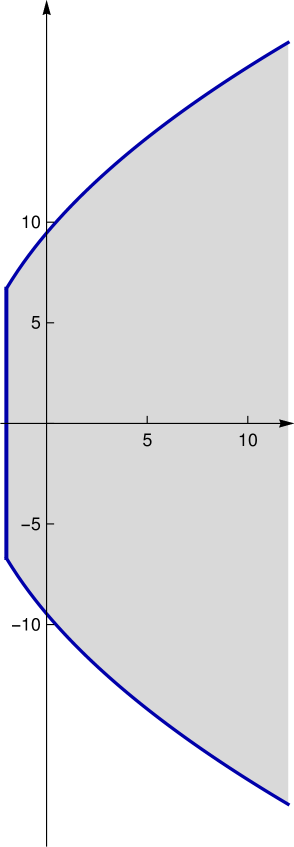
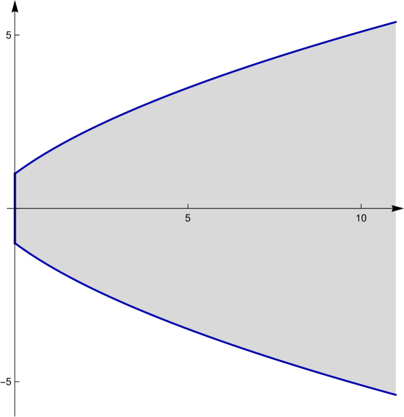
See Figure 1 for plots of the regions given
by the right-hand sides of (5.12), (5.13), (5.15).
Notice that in Theorem 5.6 (a)
we get, in fact, a family of enclosures in parabola-type regions that depend
on the choice of the parameter . By intersecting all these regions
with respect to one gets
a finer enclosure for the numerical range of .
(a) , , (b) , (c) , (d) , (e) ,
Figure 1. The plots show the regions given by the right-hand sides
of (5.12), (5.13), (5.15)
with , and for the
following cases: in (a)–(c) (, , , respectively)
and in (d), (e) (, , respectively).
Proof.
Note first, that the conditions of Theorem 3.1 are satisfied;
we point out, particularly, that by (5.11) and (2.15)
we have for each
(see Proposition 2.7), and there exists
such that . Hence, is sectorial.
Since is self-adjoint and bounded from below and the assumptions (i)–(iv)
in Theorem 5.1 hold, the latter yields .
Thus is m-sectorial and hence .
For the rest of the proof assume that and
that is bounded. For every we
have by condition (ii)
of Theorem 5.1; in particular,
and .
Hence
This implies that
(5.16)
where we have used that is a bounded operator defined on the dense
subspace of . Let .
It follows from Theorem 3.1 and (5.16) that, for every
for which , the inequalities
(5.17)
hold.
(a) Assume that .
For every we have
and, by (5.11),
(5.18)
Hence (5.17) is true for each such .
For the real part of this yields
(5.19)
To estimate further, note that the function
is strictly increasing and that
for all by (5.18).
Hence (5.17) yields
(5.20)
Now let be arbitrary.
Then (5.19) implies that .
Choose , which satisfies .
From (5.20) and we obtain the inequality
(b), (c) Assume now that .
For every we have and
. Hence (5.17) is true for ,
which, in particular, shows that
(5.21)
Note that is strictly increasing
on . Hence (5.17) and (5.11) imply that
(5.22)
Assume first that .
Now we distinguish the two cases and .
First let and . We choose
which yields
in particular, we have .
Hence (5.22) implies that
which shows that is contained in the right-hand side of (5.13).
Taking the limit we obtain this inclusion also for the case when .
The estimates for follow from the fact that the
function , has a
unique minimum at and that
as or .
and hence is contained in the right-hand side of (5.15).
Since the numerical range is a convex set, the inclusions
(5.13) and (5.15) hold also for with .
∎
Next we formulate a variant of Theorem 5.6 for the special case
when is an ordinary boundary triple.
In this case the assumptions in Theorem 5.1 imply that
is a bounded operator in ; cf. Remark 5.3.
Corollary 5.7.
Let be an ordinary boundary triple for
with corresponding Weyl function and suppose that the self-adjoint
operators and are bounded from below.
Further, assume that there exist , and
such that
Let be a bounded, everywhere defined operator in and
let be such that for all .
Then the operator in (5.2) is m-sectorial and,
in particular, the inclusion holds.
Moreover, the assertions in Theorem 5.6 (a), (b) and (c) are true.
In the following theorem we drop the assumption that is bounded from below,
but we assume that .
We remark that the condition (5.1) does no longer make sense
if is not bounded from below. Therefore we replace it by the
more appropriate condition (5.23) below.
Theorem 5.8.
Let be a quasi boundary triple for
with corresponding Weyl function . Assume that is bounded
for one (and hence for all) and that
(5.23)
for some fixed . Let be such that
(i)
for all ;
(ii)
or is self-adjoint.
Then the operator in (5.2) is closed,
the resolvent formula (5.4) holds for
all , and
(5.24)
In particular, for every interval
or there exists such that
(5.25)
Moreover, if is self-adjoint (accumulative, dissipative, respectively),
then is self-adjoint (maximal dissipative, maximal accumulative, respectively).
Further, if conditions (i) and (ii) are satisfied also for the adjoint
operator instead of , then .
It follows from this and the assumptions of the current theorem that
Corollary 4.4 can be applied. Thus is closed,
the resolvent formula (5.4) holds for
all , (5.24) is valid,
and the statement on follows. The relation (5.25)
follows from (5.23), Lemma 2.6 and (5.24).
If is symmetric (accumulative, dissipative, respectively), then it follows
as in the proof of Theorem 5.1 that is symmetric
(dissipative, accumulative, respectively).
This, together with (5.25), implies the remaining assertions.
∎
The next proposition complements Proposition 5.5.
Here we require a decay condition on the Weyl function on a set
that is sufficiently large. In later sections this is applied to,
e.g. all of or to certain sectors in the complex plane.
Proposition 5.9.
Let be a quasi boundary triple for
with corresponding Weyl function and assume that is bounded
for one (and hence for all) .
Further, let such that
(i)
for all ;
(ii)
or is self-adjoint.
Let be a set such that there exist , ,
with
Then the following assertions hold.
(a)
If there exist and such that
then is a closed extension of and
(5.26)
(b)
If there exist , and such that
(5.27)
then is a closed extension of and
(5.28)
Proof.
We prove only assertion (a); the proof of the second assertion is analogous.
Assume first that condition (i) and the first condition in (ii) are satisfied.
By the assumption on , there exists such that
. Then
implies that . It follows from Theorem 4.1
that is closed with .
If the condition (i) together with the second condition in (ii) is
satisfied then and for each
we have
;
see [22, Proposition 2.6 (iii)].
Hence, for each such we have by (i),
that is, the first condition of (ii) is satisfied as well.
∎
In the special case and with in (5.27),
Proposition 5.9 (b) reads as follows.
Corollary 5.10.
Let the assumptions be as in Proposition 5.9 and assume,
in addition, that is non-negative and that there exist
and such that
Then
6. Sufficient conditions for decay of the Weyl function
In this section we consider conditions on the quasi boundary triple
that ensure an asymptotic behaviour of the Weyl function
as required in the results of the previous section. We emphasize
that these results are also new in the settings of ordinary and generalized
boundary triples.
For the next theorem some notation for sectors in the complex plane is needed.
For
and we define the
closed sector in by
(6.1)
and we denote the corresponding complex conjugate sector in
by , that is,
Figure 2. The sectors and , defined
in (6.1) and (6.2), respectively.
In the proof of the next theorem we need the following fact
from the functional calculus for self-adjoint operators, which
is found, e.g. in [125, Theorem 5.9]:
for a self-adjoint operator and measurable functions
one has
(6.3)
If is bounded on , then the closure on the left-hand side
is not needed.
Theorem 6.1.
Let be a densely defined, closed, symmetric operator in a Hilbert space
and let be a quasi boundary triple for
with corresponding Weyl function . Moreover, assume that
(6.4)
is bounded for some and some .
Then the following assertions hold.
(a)
is bounded for all .
(b)
For all and
all
there exists such that
(6.5)
for all .
(c)
If is bounded from below, then for all
and all
there exists such that
(6.6)
for all .
Proof.
Let us first observe that is densely
defined. Indeed, with the functions and
we can use (6.3)
and (2.3) to write
Since and is dense in , it follows
that is densely defined.
By assumption (6.4) we therefore have
(6.7)
Note that also is
densely defined since
and is self-adjoint.
Moreover, set
and note that and that is bounded.
We obtain from (2.3),
(6.3) and (6.7) that
Thus is
bounded and densely defined. In particular,
(6.8)
where we have used again that .
Let and define the functions
which satisfy . The functions , and
are bounded on and
by (6.8).
Hence for each we have
(where we use (2.5) in the second equality)
(6.9)
According to (6.7) and (6.8) the terms in the square brackets
are bounded and everywhere defined operators, which are independent
of . Since is bounded on , it follows
that is a bounded, densely defined operator,
and assertion (a) is proved.
Assertions (b) and (c) follow from suitable estimates of .
Let be the spectral measure for the operator .
For all and all we have
(6.10)
In order to prove (b), fix and .
It remains to estimate the integrand of the last integral in (6.10)
uniformly in and .
To this end set .
Let , i.e.
If , then
where the right-hand side is independent of and ; by continuity this
estimate extends to .
The case can be treated analogously.
From this, together with (6.9) and (6.10), the claim of (b) follows.
To prove (c), let and ;
note that .
Let first with .
Then with the integrand of the last integral
in (6.10) can be estimated using
where we have used .
If , this and (6.10) lead to a uniform estimate
of in . If , then
with , and a uniform estimate of the last integral
in (6.10) for follows from the
previous consideration and item (b). The proof is complete.
∎
Remark 6.2.
Suppose that the assumptions of Theorem 6.1 are satisfied
for . It follows from Theorem 6.1 that
is bounded for every and that is uniformly
bounded on each sector as in the theorem.
In addition, we can show (see below) that for each as in the theorem,
(6.11)
Similarly, if is bounded from below, then
is bounded for every and is uniformly
bounded on each sector as in the theorem, and for
each such ,
and observe that by (6.9) it is sufficient to show that
It was shown in the proof of Theorem 6.1 that the integrand
is uniformly bounded for and .
Moreover, the measure is finite and the integrand converges
to as for each fixed .
Hence the dominated convergence theorem implies that
as in , which proves (6.11).
The same argument also shows (6.12).
Corollary 6.3.
Let be a quasi boundary triple for
with corresponding -field and Weyl function and
assume that the operator in (6.4)
is bounded for some and some .
Then the following assertions hold.
(a)
For all and
all
there exist and
such that
(6.13)
(6.14)
for all .
(b)
If is bounded from below, then for all
and all
there exist and such that
(6.15)
(6.16)
for all .
Proof.
(a)
First we prove (6.13).
Let and .
For with we have
for with .
Since , see (2.6),
and is bounded on the
set ,
the inequality (6.13) is proved.
The inequality in (6.14) is obtained from (6.13)
and (2.7) as follows:
(b)
Now assume that is bounded from below and set .
Let and, without loss of generality, .
Let and and define the function
where the function is defined with a cut on
the negative half-line.
The already proved item (a) implies that (6.13) is valid
for with and
some . In particular, it is true for with ,
which yields that
for all with .
Since by (2.4) the function grows at most like a power of on the
half-plane , the Phragmén–Lindelöf principle
(see, e.g. [47, Corollary VI.4.2])
implies that
It follows from this that
If we combine this with (6.13) with and ,
we obtain (6.15).
The estimate (6.16) follows from (6.15) in the
same way as in (a).
∎
The following example shows that Theorem 6.1 is sharp in a certain sense.
Example 6.4.
Let and
let be the Borel measure on that has support ,
is absolutely continuous and has density
Moreover, define
This function is the Weyl function of the following ordinary boundary triple
note that is uniquely determined by since the measure is infinite.
The operator is the multiplication operator by the independent variable.
The mapping in (6.4) with is bounded since for with
compact support we have
and the last integral converges.
Hence Theorem 6.1 yields that
One can show that the actual asymptotic behaviour of is
with a positive constant .
Hence, apart from the logarithmic factor, Theorem 6.1
yields the correct asymptotic behaviour.
Using Krein’s inverse spectral theorem (see, e.g. [92])
one can rewrite this example as a Krein–Feller operator:
with some mass distribution so that the measure becomes the
principal spectral measure of the string.
The next corollary is an immediate consequence of Theorem 6.1.
Corollary 6.5.
Let be a quasi boundary triple for
with corresponding Weyl function and assume that the operator in (6.4)
is bounded for some and some .
Then satisfies
(6.17)
for every .
Condition (6.17) says that the function belongs to
the Kac class (see, e.g. [93] for the scalar case).
Assume that satisfies (6.17) for some
and consider the integral representation
where and are bounded symmetric operators and is
an operator-valued measure (see, e.g. [116] or [23, §3.4]).
Often the measure plays the role of a spectral measure.
For each we have
It follows from [130, Lemma 3.1] and its proof that
and that
with some , which does not depend on .
Hence and
is a bounded operator.
7. Elliptic operators with non-local Robin boundary conditions
In this section we apply the results of the previous sections to
elliptic differential operators on domains whose boundaries
are not necessarily compact.
Our main focus is on operators subject to non-self-adjoint boundary conditions.
For some recent investigations of non-self-adjoint elliptic operators
we refer the reader to [40, 41, 76, 86, 115].
Let be a domain that is uniformly regular111This means
that is -smooth and that
there exists a covering of by open sets , , and
such that at most of the have a non-empty intersection,
and a family of -homeomorphisms
such that ,
the derivatives of , , and their inverses are uniformly bounded, and
covers a uniform neighbourhood of .
in the sense of [38, p. 366] and [74, page 72]; see also [20, 39].
This includes, e.g. domains with compact -smooth boundaries or compact,
smooth perturbations of half-spaces. Moreover, the class of uniformly regular
unbounded domains includes certain quasi-conical
and quasi-cylindrical domains in the sense
of [57, Definition X.6.1].
Non-self-adjoint elliptic operators with Robin boundary conditions
on such domains have been investigated recently in connection with
non-Hermitian quantum waveguides and layers;
see, e.g. [34, 35, 36, 113].
Further, let
(7.1)
be a differential expression on , where
we assume that are bounded,
have bounded, uniformly continuous derivatives on
and satisfy for all , ,
and that is real-valued; cf. [20, (S1)–(S5) in Chapter 4].
Moreover, we assume that is uniformly elliptic, i.e. there exists such that
In the following we denote by and
the Sobolev spaces of order on and , respectively.
For , where denotes
the set of -functions with compact support, let
denote the conormal derivative of at with respect to ,
where is the unit normal vector field
at pointing outwards. Then Green’s identity
(7.2)
holds for all , where the inner products are
in and , respectively.
Recall that the pair of mappings
extends by continuity to a bounded map from
onto ;
see, e.g. [74, Theorem 3.9]. The extended trace and conormal derivative
are again denoted by and
, respectively.
Moreover, Green’s identity (7.2) extends to all ;
see [74, Theorem 4.4].
In order to construct a quasi boundary triple, let us define the
operators and in via
(7.3)
and
(7.4)
Moreover, we define boundary mappings by
The assertions of the following proposition can be found in
[29, Propositions 3.1 and 3.2].
Proposition 7.1.
The operator in (7.3) is closed, symmetric and densely defined
with for in (7.4),
and the triple
is a quasi boundary triple for with the following properties.
(i)
.
(ii)
is the Neumann operator
and is the Dirichlet operator
Both operators, and , are self-adjoint and bounded from below.
(iii)
For , the associated -field satisfies
(7.5)
and the associated Weyl function is given by the Neumann-to-Dirichlet map,
(7.6)
Moreover, is a bounded, non-closed operator in
with domain such that
.
In order to apply the results of Section 5 to the quasi
boundary triple in Proposition 7.1 we prove estimates
for the Weyl function in certain sectors using Theorem 6.1.
Lemma 7.2.
Let be defined as in (6.2). Then for
each , and
there exists such that
(7.7)
Proof.
Let . Then is a positive,
self-adjoint operator in and
in is well defined, self-adjoint and positive.
It can be seen with the help of the quadratic form associated
with that and that
the -norm is equivalent to the graph norm .
Thus the identity operator provides an isomorphism between
and as well as, trivially,
between and .
By interpolation (see, e.g. [110, Theorems 5.1 and 7.7]),
the identity operator is also an isomorphism
between and
for each .
In particular,
for each . It follows from the closed graph theorem that
is bounded as an operator from to
for each such . Since the trace map is bounded from
to for each
by [74, Theorem 3.7],
it follows that
is bounded from to for each .
In particular, the operator
(7.8)
is bounded for each . By Theorem 6.1
for each , each
and each there
exists such that
holds for all .
From this the claim of the lemma follows.
∎
Remark 7.3.
Along the negative real axis the result of Lemma 7.2
can be slightly improved. It was proved in [29, Proposition 3.2 (iv)]
(using techniques from [4]) that for each
there exists such that
(7.9)
In the next theorem we apply Lemma 7.2, Remark 7.3
and the results from Section 5 to obtain m-sectorial
(self-adjoint, maximal dissipative, maximal accumulative) realizations of
subject to generalized Robin boundary conditions and also spectral enclosures
for these realizations.
Theorem 7.4.
Let be a closable operator in such that
(7.10)
Assume further that there exists such that
(7.11)
Then the operator
(7.12)
in is m-sectorial, one has ,
the resolvent formula
(7.13)
holds for all , and the following assertions are true.
(i)
If is symmetric, then is self-adjoint and bounded from below.
If is dissipative (accumulative, respectively),
then is maximal accumulative (maximal dissipative, respectively).
(ii)
If is a closable operator in that
satisfies (7.10) and (7.11) with
replaced by and
(7.14)
holds, then .
Moreover, the following spectral enclosures hold.
(iii)
If , then .
(iv)
If , is bounded and ,
then for each
there exists such that for each one has
(see Fig. 3 (a))
(v)
If , is bounded and ,
then for each there exists such that
(see Fig. 3 (b))
(vi)
If is bounded, then for each ,
and there exists such that
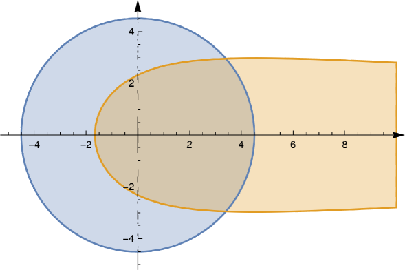
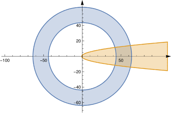
Figure 3. The plots show the regions given in Theorem 7.4 (iv), (v),
respectively, that contain for (a) and (b) ;
it is assumed that , ,
for both
cases and in (a).
Proof.
Let be a closable operator in that
satisfies (7.10) and (7.11) for some .
Let be the quasi boundary triple
in Proposition 7.1. It follows from
Lemma 7.2 that (5.1) is valid
for the corresponding Weyl function. The assumptions (i) and (iv) and
the second assumption in (v) of Theorem 5.1 are satisfied
due to the assumptions of the present theorem and the fact that
is self-adjoint and bounded from below by Proposition 7.1.
Assumption (iii) of Theorem 5.1 follows from the
last assertion of Proposition 7.1 (iii) and (7.10).
For assumption (ii) of Theorem 5.1 note that
which can be verified as in the proof of [29, Proposition 3.2 (iii)],
and use (7.10).
It follows from Proposition 7.1 that and are
bounded from below.
Thus Theorem 5.1 and Corollary 5.4
imply assertions (i)–(iii).
Moreover, Theorem 5.6 and (7.9)
yield that is m-sectorial and the assertions in items (iv) and (v);
note that the estimate for in (v) follows from taking the
estimates in Theorem 5.6 (b), (c) for all .
Finally, to prove item (vi) one combines Lemma 7.2 and
Proposition 5.9 (a) with .
∎
Remark 7.5.
(i)
The constants in items (iv)–(vi) of the above theorem depend only
on the differential expression and the domain
and on in (iv), (v) and on in (vi);
the constants are independent of the operator .
(ii)
In many cases (e.g. when is bounded), one can define
in (7.4) on the larger domain
see [22, §4.2]. In this case the extensions of the
boundary mappings and to give rise
to a generalized boundary triple, and the second condition in (7.10)
on is not needed to guarantee that the assertions of Theorem 7.4
are true for the operator
instead of (7.12). In particular, for every bounded operator
the statements (i)–(vi) in Theorem 7.4 are true.
The second condition in (7.10) is needed to obtain
the extra regularity ;
see also [1, Theorem 7.2] for a related result.
(iii)
The assertions in (iv) and (v) of Theorem 7.4 imply that the spectrum
of is contained in a parabola if and is bounded.
This is in accordance with [19, Theorem 5.14],
where the Laplacian on a bounded domain with bounded was studied.
In that paper a setting with as mentioned in the previous item
of this remark was used.
(iv)
Under the basic assumptions of Theorem 7.4 the operator
is m-sectorial and hence generates an analytic semigroup.
For the Laplacian on a bounded domain this was proved in [3]
in the setting as in (ii).
The next remark shows that the condition (7.10)
can be relaxed when an adjoint pair of boundary operators that
map into is given.
In this case the assumption
is not needed.
Remark 7.6.
Assume that and are linear operators in which satisfy
(7.15)
and
(7.16)
(7.17)
Then and have closable extensions and , respectively,
that satisfy (7.10) and (7.14).
Indeed, it follows from (7.16) and (7.17) that and
are densely defined. Hence (7.15) shows that and are closable.
This and the second condition in (7.17)
imply that is bounded
from to .
A duality argument as, e.g. in [27, Lemma 4.4]
shows that the Banach space adjoint of ,
which we denote by , is an extension of and a bounded mapping
from to .
Interpolation (see, e.g. [110, Theorems 5.1 and 7.7]) implies
that is bounded from
to .
Hence
and (7.10) is satisfied.
In a similar way one constructs an extension of that
satisfies .
The relation (7.14) is obtained by continuity.
We emphasize that in this situation replacing by in the
definition of does not change the domain of the operator.
If, for , we choose a multiplication operator by some function ,
we obtain classical Robin boundary conditions. We formulate this situation
in the following corollary, which follows from Theorem 7.4
and Remark 7.6 with being the multiplication operator
by .
Corollary 7.7.
Let be a measurable complex-valued function on such that
(7.18)
and that
(7.19)
Then the operator
in is m-sectorial, one has ,
and the resolvent formula
holds for all .
Moreover, the following assertions are true.
(i)
.
(ii)
If is real-valued, then is self-adjoint and bounded from below.
If (, respectively) for almost all ,
then is maximal accumulative (maximal dissipative, respectively).
Further, if is bounded, then the enclosures for
in Theorem 7.4(iv) and (v) hold with
replaced by .
If is bounded, then also the enclosure in Theorem 7.4(vi)
holds with replaced by .
Remark 7.8.
Condition (7.18) says that is a multiplier from
to , in the notation of
[119] written as
In certain situations there exist characterizations or sufficient conditions
for this property.
For example let
Then .
The set of multipliers can be characterized using capacities;
see [119, Theorem 3.2.2].
For the case there is a simpler characterization and for there
are simpler sufficient conditions. To this end, let us recall some notation.
Let denote the (fractional) Sobolev space (or Bessel potential space)
defined as
where is the space of tempered distributions,
is the -dimensional Fourier transform,
and is the operator of multiplication by ;
see, e.g. [58, §2.2.2 (iii)] or [119, §3.1.1].
Further, let be such that on the
unit ball, and set for .
Let
a space of functions being in only locally but in a uniform way;
see [119, p. 34].
We also set .
When , one obtains from [119, Theorem 3.2.5] that
satisfies (7.18) if and only if
(7.20)
In the case we can use [119, Theorem 3.3.1 (ii)] to provide sufficient conditions:
satisfies (7.18) if
(7.21)
The implication in the case can be shown as follows:
if and , then
by [119, Theorem 3.3.1 (ii)],
and since is continuously embedded in ,
we therefore have .
If is a domain with smooth compact boundary, then one can
characterize multipliers using charts to reduce the situation to the half-space case,
i.e. satisfies (7.18) if and only
if when ;
when , satisfies (7.18) if (7.21) holds
with replaced by .
Example 7.9.
An example of an unbounded function that satisfies (7.20) is
smoothly connected, e.g. to the zero function outside or
to periodically shifted copies of this function.
That belongs to can be seen from the fact
that it is the trace of a function that satisfies
Note that such a function also satisfies (7.19)
and hence Corollary 7.7 can be applied.
Let us consider an example in which the spectral estimates of the
previous theorem can be made more explicit.
Example 7.10.
Let ,
so that ,
and consider the negative Laplacian .
Then and
the Weyl function of the quasi boundary triple in Proposition 7.1
can be calculated explicitly,
(7.22)
see, e.g. [87, (9.65)]. Here
denotes the self-adjoint Laplacian in .
From (7.22) we obtain
(7.23)
In particular, the estimate (7.9) is satisfied with
and . Hence we can use Theorem 5.6 to obtain
a better inclusion for the numerical range.
Let be a closable operator that satisfies (7.10)
and (7.11) such that
and is bounded.
If , then for every one has
If , then
(7.24)
Note that .
If is bounded, then we can use Proposition 5.9 (a)
with to obtain the spectral enclosure
(7.25)
In the case of the Robin boundary condition,
i.e. when is a multiplication operator with a complex-valued
function , an enclosure alternative to (7.25)
can be found in [72, Theorem 2],
where the operator norm is replaced by an -norm of
with a suitably chosen .
Finally, we remark that for and close to the origin,
the enclosure (7.24) is sharper than (7.25).
If the boundary of is compact, then the differences
of the resolvents of and or , respectively,
belong to certain Schatten–von Neumann ideals as the following theorem shows.
For the case of a bounded self-adjoint operator in
the inclusions in (7.28) and (7.29) were proved
in [27, Theorem 4.10 and Corollary 4.14]; cf. also [25, 88].
Theorem 7.11.
Let be compact and let all assumptions of
Theorem 7.4 be satisfied. Then
(7.26)
and , and
(7.27)
and .
If, in addition, then
(7.28)
and , and
(7.29)
and .
Proof.
Let be the quasi boundary triple
in Proposition 7.1 and let be the corresponding -field.
Clearly, ,
and it follows from (2.3) that
for all .
Therefore we can conclude as in [25, Lemma 3.4] that
(7.30)
and for each .
Moreover, for
we have the relations
and
since maps onto .
It follows again as in [25, Lemma 3.4] that
(7.31)
and for each .
From (7.30) we obtain with the help of Proposition 4.7
the assertions (7.26) and (7.27).
For , Proposition 4.8,
(7.30) and (7.31) yield (7.28)
and (7.29).
∎
Remark 7.12.
Note that the statement of Theorem 7.11
can be refined if we replace the usual Schatten–von Neumann classes
by the weak Schatten–von Neumann classes ,
which are discussed in Remark 4.9.
In this case one can allow to be equal to , or ,
respectively; cf. [27, Section 4.2] and [28, Section 3].
8. Schrödinger operators with -interaction on hypersurfaces
In this section we provide some applications of the results in
Sections 4, 5 and 6
to Schrödinger operators with -interaction supported on a
smooth, not necessarily bounded hypersurface in .
To be more specific, we consider operators associated with the
formal differential expression
where is a complex constant or a complex-valued function on ,
the strength of the -interaction.
The spectral theory of such operators is a prominent subject in
mathematical physics; see the review paper [62], the monograph [67],
and the references therein. The largest part of the existing literature
(see, e.g. [37, 64, 66, 68, 69, 111, 118])
is devoted to the case of a real interaction strength .
However, there has been recent interest in non-real ;
see, e.g. [72, 98].
In what follows, let be a uniformly regular, bounded or
unbounded domain in (see Section 7)
with boundary .
Furthermore, let
be its complement in . We write
for , where .
By the same reason as in Section 7, the trace and the
normal derivative extend to continuous linear mappings
Both the above mappings are surjective onto .
Furthermore, we introduce an operator in by
(8.1)
On we define boundary mappings and by
(8.2)
here stand
for the normal derivatives of on two
opposite faces of with the normals pointing outwards ;
note that the outer unit normal vector fields and
of and , respectively, satisfy
for all . Moreover, consider the symmetric operator
in defined as
(8.3)
In the following proposition we state that
is a quasi boundary triple for and we formulate
properties of this triple and of the associated -field
and Weyl function. This proposition is analogous to
Proposition 7.1 and can be proved in a similar way;
see the proofs of [29, Propositions 3.1 and 3.2].
Note that in the case of a compact , the statements and proofs
of the next proposition and further details can be found in [26, §3]
and [27, §3.1].
Proposition 8.1.
The operator in (8.3)
is closed, symmetric and densely defined
with for in (8.1), and the
triple
is a quasi boundary triple for with the following properties.
(i)
.
(ii)
is the free Laplace operator
and is the orthogonal sum of the Dirichlet Laplacians on
and , respectively,
Both operators, and ,
are self-adjoint and non-negative in .
(iii)
For all the associated -field satisfies
(8.4)
and the associated Weyl function is given by:
(8.5)
Moreover, is a bounded, non-closed operator in
with domain such that .
The following lemma ensures the decay of the Weyl function in (8.5).
For the definition of the exterior sector we refer to (6.2).
Lemma 8.2.
Let denote the Weyl function in (8.5).
Then for all , , and
there exists a constant such that
(8.6)
Proof.
Let be the quasi boundary triple in
Proposition 8.1. Recall that ;
in particular,
and for all by the
definition of the Sobolev spaces.
Hence by the closed graph theorem, is bounded as
an operator from to for each .
Since the trace map is bounded from to
for each , it follows that
is bounded
from to for each .
Therefore the operator
is bounded for each .
By Theorem 6.1 it follows that for each ,
each and each
there exists such that
holds for all .
From this the claim of the lemma follows.
∎
Remark 8.3.
It can be shown as in [26, Proposition 3.2 (iii)] that
(8.7)
where and are the Weyl functions from Section 7
for on and , respectively.
Remark 7.3 implies that for each there
exist such that
Since for ,
it follows from [10, Corollaries I.2.4 and I.3.2] that
Hence for each
there exists such that
From Lemma 8.2, Remark 8.3 and the
results of Section 5 we obtain the following consequences
for Schrödinger operators with -potentials supported on ;
cf. the proof of Theorem 7.4 and Corollary 7.7.
Note that the assumptions of the next theorem allow certain classes
of unbounded functions ; cf. Remark 7.8.
Theorem 8.4.
Let be a measurable complex-valued function such that
(8.8)
and that
Then the Schrödinger operator with -interaction of strength
supported on ,
(8.9)
in
is m-sectorial, one has , the resolvent formula
(8.10)
holds for all , and the following assertions are true.
(i)
.
(ii)
If is real-valued, then is self-adjoint and bounded from below.
If (, respectively) for almost all ,
then is maximal accumulative (maximal dissipative, respectively).
Moreover, the following spectral enclosures hold.
(iii)
If , then .
(iv)
If is bounded and , then for each there exists such that
for each ,
(v)
If is bounded and , then for each there exists such that
(vi)
If is bounded, then for each ,
and there exists such that
Let us illustrate the obtained spectral estimates in an example.
Example 8.5.
Consider the case
that is, , which we
identify with .
It follows from (8.7) and (7.22) that
and hence
In particular, the estimate (5.11) is satisfied with
and .
In analogy to Example 7.10, this observation can be used
to obtain several better enclosures for the spectrum and
numerical range of the operator .
Let satisfy the conditions of Theorem 8.4 and
let be bounded.
If , then for every one has
If , then
If, in addition, is bounded, then by Proposition 5.9 (a)
with the spectrum of satisfies the enclosure
We now have a closer look at the special case of a compact hypersurface
and bounded . For this case certain refined bounds for the
function from the recent work [75] are available and can be combined
with the results in the abstract part of this paper in order to obtain
the spectral bounds for that are contained in the next theorem.
We remark that [75]
contains further bounds in space dimension two and in the special case
when is a convex domain, which could be combined with our theorems;
however, we do not include this in the next theorem.
Theorem 8.6.
Let be compact and let be a complex-valued
function which satisfies (8.8).
Then there exist constants , which are independent of ,
such that the spectrum of satisfies
(8.11)
where
(a)
(b)
Figure 4. The sets (blue) and (yellow)
in Theorem 8.6 for (a) and (b) , respectively,
where in (a),
and and in (b).
Proof.
By [75, Theorems 1.2 and 1.3] there exist constants
(the constants here differ from the ones in [75]
by a factor ) such that
hold for all .
Thanks to condition (8.8) we can view the multiplication
with as an operator in with domain
and range contained in .
Hence, by Theorem 4.1, any point
for which at least one of the above two upper bounds
on is strictly less than one
belongs to the resolvent set of .
Thus, the enclosure in (8.11) follows.
∎
Furthermore, we obtain certain Schatten–von Neumann estimates for the
difference of the resolvents of and the free Laplacian.
They are analogues of the first and the third estimates in
Theorem 7.11, and the proofs are analogous, where one uses the relations
and
Theorem 8.7.
Let all assumptions of Theorem 8.4 be satisfied.
Moreover, assume that is compact. Then
(8.12)
and all .
If, in addition, is bounded, then
(8.13)
and all .
Remark 8.8.
In the same way as in Remark 7.12, we can reformulate
Theorem 8.7 for weak Schatten–von Neumann classes.
In this setting the endpoints for the intervals
of admissible values of can be included in
both (8.12) and (8.13); cf. [26, Section 4.2].
Remark 8.9.
In the case of a real, bounded coefficient , in space dimensions 2 and 3 the
previous theorem can be used in order to derive existence and completeness
of wave operators for the scattering pair .
In space dimension 2, the same is true for certain unbounded ;
cf. Example 7.9.
Let us also mention [118] where Schatten–von Neumann properties
were proved for certain -interactions with unbounded real-valued coefficients.
Finally, in the last theorem of this section we show that in two space dimensions
for small enough the spectrum of
outside is contained in a disc with radius that
converges to exponentially as and that
in higher dimensions has no spectrum
outside if is small enough.
The result in two dimensions agrees well with the asymptotic expansion
in [99] in the self-adjoint setting.
Related conditions for absence of non-real eigenvalues in higher dimensions
for Schrödinger operators with complex-valued regular potentials can be found in [70, 71].
In the self-adjoint setting absence of negative eigenvalues for
small enough is also a consequence of the Birman–Schwinger bounds in [37];
see also [63].
Theorem 8.10.
Let be compact and let be a
complex-valued function that satisfies (8.8).
Then , and the following statements hold.
The statement about the essential spectrum follows
directly from Theorem 8.7.
(i)
Assume that and
let .
It follows from Theorem 8.6 that and hence
which implies that
(ii)
Since the maximum of the function , is
(attained at ), it follows that
If
then
for every , and Theorem 8.6
implies that .
Together with the relation
this shows that .
∎
9. Infinitely many point interactions on the real line
In this section we provide applications of the results in
Section 5
to Hamiltonians with non-local, non-Hermitian
interactions supported on a discrete set of points ,
where is a strictly increasing sequence of real numbers.
The investigation of such Hamiltonians has been initiated
almost a century ago in [105] for periodically distributed, local,
Hermitian point -interactions.
Classical results are summarized in the monograph [7];
see also the references therein and [97, 102].
More recently, non-Hermitian interactions attracted attention (see [6, 9])
and also non-local interactions were studied; see [9, 107].
Throughout this section we make the assumption
(9.1)
in particular, the sequence does not have a finite accumulation point.
We remark that this assumption can be avoided by using the methods of [8, 101],
but we do not focus on this here.
For each interval we denote by the
usual Sobolev space on of second order.
Moreover, we set for and introduce
equipped with the norm
(9.2)
In order to construct a boundary triple which is suitable for the parameterization
of Hamiltonians with interactions supported on ,
we define operators and in by
(9.3)
and
(9.4)
that is, consists of all
such that for all .
Moreover, for we define
(9.5)
In fact, and are boundary mappings for an
ordinary boundary triple, as the following proposition shows;
see also [100, Proposition 7 (i)] where a very similar boundary triple
was constructed.
Proposition 9.1.
The operator in (9.3) is closed, symmetric and densely defined
with for in (9.4), and the triple
is an ordinary boundary triple for with the following properties.
(i)
is given by
(9.6)
and is given by
(9.7)
(ii)
For the associated -field
acts as
(9.8)
and the associated Weyl function satisfies
(9.9)
Proof.
Let us first check that and are well-defined mappings
from to . For this we make use of the following estimate,
which can be found in, e.g. [106, Lemma 8]:
if is a compact interval then for each one has
(9.10)
The same estimate holds for replaced by .
From (9.1) we obtain that
for each , and (9.10) yields
for all .
Hence for all .
Similarly, using (9.10) for replaced by
we get for all .
To show that is a boundary triple for ,
let us verify the conditions of Theorem 2.3.
In fact, it is clear that is given by
the operator in (9.6), which is self-adjoint.
Moreover, for all we have
Furthermore, the pair of mappings
has a
dense range since it can be checked easily that all pairs of
unit sequences , , belong to the range.
It follows from Theorem 2.3 that is closed
with and that
is a quasi boundary triple for .
In order to conclude that is even an
ordinary boundary triple, let us verify that the operator is closed.
To this end define a mapping
For all we have
where we have used (9.10) with . Therefore is a bounded operator and,
hence, its kernel, which equals , is closed in .
Equivalently, equipped with the norm of is complete.
It follows from [129, Satz 6.24], its proof and (9.1) that
for each there exists such that for all
one has
This implies that is also complete when equipped
with the graph norm of , that is, is a closed operator.
Hence is an ordinary boundary triple for .
The remaining assertion (9.7) in (i) is obvious.
For the assertions in (ii) let .
According to [129, Satz 11.26] or [127, page 190] we have
Hence for each compactly supported and
each we obtain from (2.3)
and the definition of that
where we have used that .
This proves (9.8).
With the definition of also relation (9.9) follows.
∎
Next we use the representation of the Weyl function in (9.9)
to estimate its norm.
Lemma 9.2.
The Weyl function associated with the boundary triple in
Proposition 9.1 satisfies
(9.11)
for all .
In particular, the following estimates hold.
Recall that for the
operator has the explicit representation (9.9).
In order to estimate its norm, we make use of the Schur test;
see, e.g. [129, Korollar 6.7].
For this note that holds for all and, thus,
Since the last term is finite and the same estimate holds by symmetry
when the roles of and are interchanged, the Schur test can be
applied and yields (9.11).
The statement (i) is a direct consequence of the estimate in (9.11)
and the monotonicity properties of the function .
For the remaining statement (ii) we calculate
(9.13)
By symmetry it is clear that it suffices to consider
with .
Since the function
has no local extremum, the minimum in (9.13) will be attained on the
boundary of . Let us first consider the
case when . Writing with ,
for with we have
(9.14)
and the right-hand side will be minimal if and only if
is minimal.
The latter happens for .
Plugging this into (9.14) and using elementary
trigonometric identities we obtain the claimed expression for .
The case can be treated analogously
with replaced by , and for we have
We are now able to formulate consequences of the results in
Section 5. The assertions of the next theorem follow directly
from Lemma 9.2 in combination with Corollary 5.7,
Proposition 5.9 (a), [56, Proposition 1.4 (i)]
and the fact that is an ordinary boundary triple.
Theorem 9.3.
Let be a closed operator in .
Then the operator
(9.15)
in is closed, the resolvent formula
holds for all and
the following assertions are true.
(i)
If is self-adjoint, then is self-adjoint.
If is maximal dissipative (maximal accumulative, respectively),
then is maximal accumulative (maximal dissipative, respectively).
(ii)
.
Assume, additionally, that
and let be such that
Then the operator is m-sectorial;
in particular the inclusion holds,
and for any and
the following assertions are true.
Finally, we remark that the class of Hamiltonians under consideration in this
section includes Schrödinger operators in with local point
-interactions supported on the set , with possibly non-real coupling constants.
Such operators are obtained by choosing
with for . The constant can be viewed as
intensity (or strength) of the point -interaction supported on ;
cf. [7, Chapter III.2].
10. Quantum graphs with -type vertex couplings
In this section we apply the results of the abstract part of this
paper to Laplacians on metric graphs. For a survey on this actively
developing field and references we refer the reader to the monograph [32]
and the survey articles [31, 104, 106]. In the present section we
consider the Laplacian on a finite, not necessarily compact metric graph,
equipped with or more general non-self-adjoint vertex couplings;
for further recent work on non-self-adjoint quantum graphs see [89, 90, 126].
Furthermore, for the treatment of quantum graphs via boundary triples and
similar techniques we refer to, e.g. [46, 59, 61, 109, 120, 123].
Let be a finite graph consisting of a finite set of vertices
and a finite set of edges, where we allow infinite edges,
i.e. edges ‘connecting a vertex to a point ’. Without loss of
generality we assume that there are no vertices of degree 0,
i.e. each vertex belongs to at least one edge, and that does not contain loops,
i.e. no edge connects a vertex to itself; this can always be achieved by
introducing additional vertices to the graph.
We equip each finite edge with a length and
identify it with the interval .
Moreover, we identify each infinite edge with the interval .
This identification gives rise to a natural metric on and to a natural space on .
For a vertex and an edge we write
or if originates or terminates, respectively, at ,
and we occasionally simply write if one of these two properties holds.
For each vertex we denote by the vertex degree,
that is, the number of edges which originate from or terminate at .
In we consider the Laplace differential expression
where denotes the restriction of to the edge .
In the following we write ,
, for the orthogonal sum of the usual Sobolev spaces on the edges of .
We say that a function is continuous at a vertex
whenever and imply that the values of
and at coincide. We define
Note that for we can just write for the evaluation of
at a vertex . For and a vertex we write
In order to construct an ordinary boundary triple let us consider the operators
(10.1)
and
(10.2)
in . Moreover, we choose an enumeration
of the vertex set and define mappings
by
The mappings and give rise to an ordinary boundary triple
with finite-dimensional boundary space. The following proposition is a
consequence of Theorem 2.3 and some elementary calculations.
It can also be derived from [60, Lemma 2.14 and Theorem 2.16].
For the convenience of the reader we provide its proof below.
Proposition 10.1.
The operator in (10.1) is closed, symmetric and densely defined
with for in (10.2), and the triple
is an ordinary boundary triple for with the following properties.
(i)
coincides with the standard
(or Kirchhoff) Laplacian
(10.3)
and coincides with the Dirichlet Laplacian
In particular, and are both self-adjoint and non-negative operators in .
(ii)
For , the corresponding -field is given by
(10.4)
where is any function that
satisfies , and the corresponding Weyl function is given by
(10.5)
For each
we have
(10.6)
Proof.
Let us verify the conditions of Theorem 2.3.
Note first that clearly equals the standard
Laplacian (10.3), which is self-adjoint in .
Moreover, it can easily be seen by explicit construction that the
pair is surjective.
Finally, let us verify the abstract Green identity.
For integration by parts yields
From Theorem 2.3 it follows that is closed, densely defined
and symmetric with and that
is an ordinary boundary triple for .
Assertion (i) and the identities (10.4), (10.5)
are obvious from the definition of the mappings .
It remains to verify the representation of in (10.6).
To this end fix
and denote by the Dirichlet-to-Neumann map corresponding to the
equation on the interval ;
if is finite then is the matrix satisfying
(10.7)
for each with ;
if is infinite then is the scalar function satisfying
(10.8)
for each with .
Let us define the matrix by
(10.9)
We show that . Indeed, let .
Then for we have
where we have used that does not contain loops.
Taking (10.7) and (10.8) into account we obtain that
which implies that .
Note that can be calculated explicitly and is given by the expressions
Plugging these representations into (10.9) we arrive
at (10.6).
∎
The next lemma provides a decay property of the Weyl function.
Lemma 10.2.
Let be the Weyl function corresponding to the boundary triple
in Proposition 10.1. Then for each
and there exists such that
Let and . If
for , then within
the sector .
In particular, tends to , and thus
for all as , and the convergence is uniform in .
Hence it follows from (10.6) that
uniformly as , . It follows that
(10.11)
uniformly as , .
Let be arbitrary. Since the matrix
is positive definite with smallest eigenvalue greater than or equal to 1,
it follows from (10.11) that there exists such
that the smallest eigenvalue of
satisfies
for all with . Thus we obtain that
(10.12)
for all with .
On the other hand, since is
continuous on the compact set
there exists with
(10.13)
With the claim of the lemma follows
from the inequalities (10.12) and (10.13).
∎
The assertions of the following theorem are direct consequences of
Proposition 10.1, Lemma 10.2 and Corollary 5.7.
For characterizations of self-adjoint vertex conditions for Laplacians on
metric graphs we refer the reader to [45, 103].
Theorem 10.3.
Let . Then the operator
(10.14)
in is m-sectorial, one has ,
the resolvent formula
holds for all
and the following assertions are true.
(i)
is self-adjoint if and only if the matrix is Hermitian.
Moreover, is maximal dissipative (maximal accumulative, respectively)
if and only if is accumulative (dissipative, respectively).
Note that the operator satisfies local matching conditions at all
vertices if and only if the matrix is diagonal, .
In this case consists of all functions
such that
holds for . These conditions describe -couplings
of strengths . They have been studied extensively in the literature in
the self-adjoint case, i.e. for real ;
see, e.g. [32, 60, 65, 94, 106].
Remark 10.5.
In more specific situations the spectral estimates in Theorem 10.3
can be made more explicit. Let, for instance, be combinatorially equal
to the complete graph with vertices, that is,
each two vertices are connected by precisely one edge;
in particular, for .
Moreover, let be equilateral with for all .
It follows from (10.6) that the Weyl function corresponding
to the boundary triple in Proposition 10.1 satisfies
A straightforward calculation yields that is given by
where
Since in this case is a special case of a circulant matrix,
its norm can be calculated and estimated explicitly for .
The following example shows that the abstract spectral estimate in
Corollary 5.10 cannot be improved in general.
Example 10.6.
Let be a star graph consisting of infinite edges,
i.e. each edge of can be parameterized by the interval
and there exists only one vertex , which satisfies for all .
Then for the functions in the domain of the operator
in (10.14) are continuous at and satisfy the condition
If with then has as its
only non-real eigenvalue, as an explicit calculation shows.
On the other hand, by Proposition 10.1 (ii) we
obtain that
for all , and
Corollary 5.10 yields that
JB, VL and JR gratefully acknowledge financial support by
the Austrian Science Fund (FWF), grant no. P 25162-N26.
VL acknowledges the support of the Czech Science Foundation (GAČR),
grant no. 17-01706S
and also of the support of the Austria–Czech Republic Mobility Programme,
grant no. 7AMB17AT022.
References
[1]
H. Abels, G. Grubb and I. Wood,
Extension theory and Kreĭn-type resolvent formulas for nonsmooth boundary value problems,
J. Funct. Anal.266 (2014), 4037–4100.
[2]
A. A. Abramov, A. Aslanyan and E. B. Davies,
Bounds on complex eigenvalues and resonances,
J. Phys. A34 (2001), 57–72.
[3]
M. Adler, M. Bombieri and K.-J. Nagel,
Perturbation of analytic semigroups and applications to partial differential equations,
J. Evol. Equ.17 (2017), 1183–1208.
[4]
S. Agmon,
On the eigenfunctions and on the eigenvalues of general elliptic boundary value problems,
Commun. Pure Appl. Math.15 (1962), 119–147.
[5] S. Albeverio, J. F. Brasche, M. M. Malamud and H. Neidhardt,
Inverse spectral theory for symmetric operators with several gaps: scalar-type Weyl functions,
J. Funct. Anal.228 (2005), 144–188.
[6]
S. Albeverio, S.-M. Fei and P. Kurasov,
Point interactions: -Hermiticity and reality of the spectrum,
Lett. Math. Phys.59 (2002), 227–242.
[7]
S. Albeverio, F. Gesztesy, R. Høegh-Krohn and H. Holden,
Solvable Models in Quantum Mechanics. With an appendix by Pavel Exner.
AMS Chelsea Publishing, 2005.
[8]
S. Albeverio, A. Kostenko and M. M. Malamud,
Spectral theory of semibounded Sturm–Liouville operators with local
interactions on a discrete set,
J. Math. Phys.51 (2010), 102102, 24 pp.
[9]
S. Albeverio and L. Nizhnik,
Schrödinger operators with nonlocal point interactions,
J. Math. Anal. Appl.332 (2007), 884–895.
[10]
T. Ando,
Topics on operator inequalities.
Division of Applied Mathematics, Research Institute of Applied Electricity,
Hokkaido University, Sapporo, 1978.
[11]
W. Arendt and A. F. M. ter Elst,
The Dirichlet-to-Neumann operator on rough domains,
J. Differential Equations251 (2011), 2100–2124.
[12]
W. Arendt and A. F. M. ter Elst,
The Dirichlet-to-Neumann operator on exterior domains,
Potential Anal.43 (2015), 313–340.
[13]
W. Arendt, A. F. M. ter Elst, J. B. Kennedy and M. Sauter,
The Dirichlet-to-Neumann operator via hidden compactness,
J. Funct. Anal.266 (2014), 1757–1786.
[14]
Yu. Arlinskii,
Abstract boundary conditions for maximal sectorial extensions of sectorial operators,
Math. Nachr.209 (2000), 5–36.
[15]
Yu. Arlinskiĭ,
Boundary triplets and maximal accretive extensions of sectorial operators,
in: Operator Methods for Boundary Value Problems,
London Math. Soc. Lecture Note Series, vol. 404, 2012, pp. 35–72.
[16]
Yu. Arlinskiĭ, Y. Kovalev and E. Tsekanovskii,
Accretive and sectorial extensions of nonnegative symmetric operators,
Complex Anal. Oper. Theory6 (2012), 677–718.
[17]
Yu. Arlinskiĭ and A. B. Popov,
On m-accretive extensions of a sectorial operator. [Russian]
Mat. Sb.204 (2013), 3–40;
English translation: Sb. Math.204 (2013), 1085–1121.
[18]
Yu. Arlinskiĭ and A. Popov,
On m-sectorial extensions of sectorial operators,
Zh. Mat. Fiz. Anal. Geom.13 (2017), 205–241.
[19]
W. Bade and R. Freeman,
Closed extensions of the Laplace operator determined by a general class of boundary conditions,
Pacific J. Math.12 (1962), 395–410.
[20]
R. Beals,
Non-local boundary value problems for elliptic operators,
Amer. J. Math.87 (1965), 315–362.
[21]
J. Behrndt, G. Grubb, M. Langer and V. Lotoreichik,
Spectral asymptotics for resolvent differences of elliptic operators with
and -interactions on hypersurfaces,
J. Spectr. Theory5 (2015), 697–729.
[22]
J. Behrndt and M. Langer,
Boundary value problems for elliptic partial differential operators on bounded domains,
J. Funct. Anal.243 (2007), 536–565.
[23]
J. Behrndt and M. Langer,
On the adjoint of a symmetric operator,
J. London Math. Soc. (2)82 (2010), 563–580.
[24]
J. Behrndt and M. Langer,
Elliptic operators, Dirichlet-to-Neumann maps and quasi boundary triples,
in: Operator Methods for Boundary Value Problems,
London Math. Soc. Lecture Note Series, vol. 404, 2012, pp. 121–160.
[25]
J. Behrndt, M. Langer, I. Lobanov, V. Lotoreichik and I. Yu. Popov,
A remark on Schatten–von Neumann properties of resolvent differences of
generalized Robin Laplacians on bounded domains,
J. Math. Anal. Appl.371 (2010), 750–758.
[26]
J. Behrndt, M. Langer and V. Lotoreichik,
Schrödinger operators with and -potentials
supported on hypersurfaces,
Ann. Henri Poincaré14 (2013), 385–423.
[27]
J. Behrndt, M. Langer and V. Lotoreichik,
Spectral estimates for resolvent differences of self-adjoint elliptic operators,
Integral Equations Operator Theory77 (2013), 1–37.
[28]
J. Behrndt, M. Langer and V. Lotoreichik,
Trace formulae and singular values of resolvent power differences of
self-adjoint elliptic operators,
J. London Math. Soc. (2)88 (2013), 319–337.
[29]
J. Behrndt, M. Langer, V. Lotoreichik and J. Rohleder,
Quasi boundary triples and semibounded self-adjoint extensions,
Proc. Roy. Soc. Edinburgh Sect. A147 (2017), 895–916.
[30]
J. Behrndt and J. Rohleder,
Spectral analysis of selfadjoint elliptic differential operators, Dirichlet-to-Neumann maps,
and abstract Weyl functions,
Adv. Math.285 (2015), 1301–1338.
[31]
G. Berkolaiko,
An elementary introduction to quantum graphs,
in: Geometric and Computational Spectral Theory,
Contemp. Math., vol. 700, Amer. Math. Soc.,
Providence, RI, 2017, pp. 41–72.
[32]
G. Berkolaiko and P. Kuchment,
Introduction to Quantum Graphs,
Mathematical Surveys and Monographs, vol. 186,
American Mathematical Society, Providence, RI, 2013.
[33]
M. Sh. Birman and M. Z. Solomjak,
Asymptotic behavior of the spectrum of variational problems on solutions of
elliptic equations in unbounded domains,
Funktsional. Anal. i Prilozhen.14 (1980), 27–35 [Russian];
English translation: Funct. Anal. Appl.14 (1981), 267–274.
[34]
D. Borisov and D. Krejčiřík,
-symmetric waveguides,
Integral Equations Operator Theory62 (2008), 489–515.
[35]
D. Borisov and D. Krejčiřík,
The effective Hamiltonian for thin layers with non-Hermitian Robin-type boundary conditions,
Asymptot. Anal.76 (2012), 49–59.
[36]
D. Borisov and M. Znojil,
On eigenvalues of a -symmetric operator in a thin layer [Russian],
Mat. Sb.208 (2017), 3–30;
English translation: Sb. Math.208 (2017), 173–199.
[37]
J. F. Brasche, P. Exner, Yu. A. Kuperin and P. Šeba,
Schrödinger operators with singular interactions,
J. Math. Anal. Appl.184 (1994), 112–139.
[38]
F. E. Browder,
Estimates and existence theorems for elliptic boundary value problems,
Proc. Nat. Acad. Sci. U.S.A.45 (1959), 365–372.
[39]
F. E. Browder,
On the spectral theory of elliptic differential operators. I,
Math. Ann.142 (1961), 22–130.
[40]
B. M. Brown, G. Grubb and I. G. Wood,
-functions for closed extensions of adjoint pairs of
operators with applications to elliptic boundary problems,
Math. Nachr.282 (2009), 314–347.
[41]
B. M. Brown, M. Marletta, S. Naboko and I. G. Wood,
Boundary triplets and -functions for non-selfadjoint operators,
with applications to elliptic PDEs and block operator matrices,
J. London Math. Soc. (2)77 (2008), 700–718.
[42]
B. M. Brown, M. Marletta, S. Naboko and I. Wood,
Inverse problems for boundary triples with applications,
Studia Math.237 (2017), 241–275.
[43]
V. M. Bruk,
A certain class of boundary value problems with a spectral parameter in the boundary condition,
Mat. Sb. (N.S.)100 (142) (1976), 210–216.
[44]
J. Brüning, V. Geyler and K. Pankrashkin,
Spectra of self-adjoint extensions and applications to solvable Schrödinger operators,
Rev. Math. Phys.20 (2008), 1–70.
[45]
R. Carlson,
Adjoint and self-adjoint differential operators on graphs,
Electron. J. Differential Equations1998, no. 6, 10 pp.
[46]
K. D. Cherednichenko, A. V. Kiselev and L. O. Silva,
Functional model for extensions of symmetric operators and applications to scattering theory,
to appear in Netw. Heterog. Media,
arXiv:1703.06220.
[47]
J. B. Conway,
Functions of One Complex Variable I, Second edition.
Graduate Texts in Mathematics, vol. 11, Springer, 1978.
[48]
J.-C. Cuenin,
Eigenvalue bounds for Dirac and fractional Schrödinger operators with complex potentials,
J. Funct. Anal.272 (2017), 2987–3018.
[49]
J.-C. Cuenin and C. Tretter,
Non-symmetric perturbations of self-adjoint operators,
J. Math. Anal. Appl.441 (2016), 235–258.
[50]
E. B. Davies,
Non-self-adjoint differential operators,
Bull. London Math. Soc.34 (2002), 513–532.
[51]
M. Demuth, M. Hansmann and G. Katriel,
On the discrete spectrum of non-selfadjoint operators,
J. Funct. Anal.257 (2009), 2742–2759.
[52]
V. A. Derkach, S. Hassi, M. M. Malamud and H. de Snoo,
Boundary relations and their Weyl families,
Trans. Amer. Math. Soc.358 (2006), 5351–5400.
[53]
V. A. Derkach, S. Hassi, M. M. Malamud and H. de Snoo,
Boundary relations and generalized resolvents of symmetric operators,
Russ. J. Math. Phys.16 (2009), 17–60.
[54]
V. A. Derkach, S. Hassi, M. M. Malamud and H. de Snoo,
Boundary triplets and Weyl functions. Recent developments,
in: Operator Methods for Boundary Value Problems,
London Math. Soc. Lecture Note Series, vol. 404, 2012, pp. 161–220.
[55]
V. A. Derkach and M. M. Malamud,
Generalized resolvents and the boundary value problems for Hermitian operators with gaps,
J. Funct. Anal.95 (1991), 1–95.
[56]
V. A. Derkach and M. M. Malamud,
The extension theory of Hermitian operators and the moment problem,
J. Math. Sci.73 (1995), 141–242.
[57]
D. E. Edmunds and W. D. Evans,
Spectral Theory and Differential Operators.
Oxford Mathematical Monographs. The Clarendon Press, Oxford University Press,
New York, 1987.
[58]
D. E. Edmunds and H. Triebel,
Function Spaces, Entropy Numbers, Differential Operators.
Cambridge Tracts in Mathematics, vol. 120,
Cambridge University Press, Cambridge, 1996.
[59]
Y. Ershova, I. Karpenko and A. Kiselev,
Isospectrality for graph Laplacians under the change of coupling at graph vertices,
J. Spectr. Theory6 (2016), 43–66.
[60]
Y. Ershova and A. Kiselev,
Trace formulae for graph Laplacians with applications to recovering matching conditions,
Methods Funct. Anal. Topology18 (2012), 343–359.
[61]
Y. Ershova and A. Kiselev,
Trace formulae for Schrödinger operators on metric graphs with
applications to recovering matching conditions,
Methods Funct. Anal. Topology20 (2014), 134–148.
[62]
P. Exner,
Leaky quantum graphs: a review,
in: Analysis on Graphs and its Applications.
Selected papers based on the Isaac Newton Institute for Mathematical Sciences programme,
Cambridge, UK, 2007, Proc. Symp. Pure Math.77 (2008), 523–564.
[63]
P. Exner and M. Fraas,
On geometric perturbations of critical Schrödinger operators with
a surface interaction,
J. Math. Phys.50 (2009), 112101, 12 pp.
[64]
P. Exner and T. Ichinose,
Geometrically induced spectrum in curved leaky wires,
J. Phys. A34 (2001), 1439–1450.
[65]
P. Exner and M. Jex,
On the ground state of quantum graphs with attractive -coupling,
Phys. Lett. A376 (2012), 713–717.
[66]
P. Exner and S. Kondej,
Bound states due to a strong -interaction supported by a curved surface,
J. Phys. A36 (2003), 443–457.
[67]
P. Exner and H. Kovařík,
Quantum Waveguides,
Springer, Heidelberg, 2015.
[68]
P. Exner and J. Rohleder,
Generalized interactions supported on hypersurfaces,
J. Math. Phys.57 (2016), 041507, 23 pp.
[69]
P. Exner and K. Yoshitomi,
Asymptotics of eigenvalues of the Schrödinger operator with a
strong -interaction on a loop,
J. Geom. Phys.41 (2002), 344–358.
[70]
L. Fanelli, D. Krejčiřík and L. Vega,
Spectral stability of Schrödinger operators with subordinated complex potentials,
J. Spectr. Theory, to appear,
arXiv:1506.01617.
[71]
R. L. Frank,
Eigenvalue bounds for Schrödinger operators with complex potentials,
Bull. Lond. Math. Soc.43 (2011), 745–750.
[72]
R. L. Frank,
Eigenvalues of Schrödinger operators with complex surface potentials,
in: Functional Analysis and Operator Theory for Quantum Physics,
Europ. Math. Soc., Zürich, 2017, pp. 245–259.
[73]
R. Freeman,
Closed extensions of the Laplace operator determined by a
general class of boundary conditions, for unbounded regions,
Pacific J. Math.12 (1962), 121–135.
[74]
R. Freeman,
Closed operators and their adjoints associated with
elliptic differential operators,
Pacific J. Math.22 (1967), 71–97.
[75]
J. Galkowski and H. F. Smith,
Restriction bounds for the free resolvent and resonances in lossy scattering,
Int. Math. Res. Notices16 (2015), 7473–7509.
[76]
F. Gesztesy, Y. Latushkin, M. Mitrea and M. Zinchenko,
Nonselfadjoint operators, infinite determinants, and some applications,
Russ. J. Math. Phys.12 (2005), 443–471.
[77]
F. Gesztesy and M. Mitrea,
Generalized Robin boundary conditions, Robin-to-Dirichlet maps, Kreĭn-type
resolvent formulas for Schrödinger operators on bounded Lipschitz domains,
in: Perspectives in Partial Differential Equations, Harmonic Analysis and Applications,
Proc. Sympos. Pure Math., vol. 79, Amer. Math. Soc., Providence, RI, 2008,
pp. 105–173.
[78]
F. Gesztesy and M. Mitrea,
A description of all self-adjoint extensions of the
Laplacian and Kreĭn-type resolvent formulas on non-smooth domains,
J. Anal. Math.113 (2011), 53–172.
[79]
F. Gesztesy, M. Mitrea and M. Zinchenko,
Variations on a theme of Jost and Pais,
J. Funct. Anal.253 (2007), 399–448.
[80]
F. Gesztesy, M. Mitrea and M. Zinchenko,
On Dirichlet-to-Neumann maps and some applications to modified Fredholm determinants,
in: Methods of Spectral Analysis in Mathematical Physics,
Oper. Theory Adv. Appl., vol. 186, Birkhäuser Verlag, Basel, 2009,
pp. 191–215.
[81]
I. C. Gohberg and M. G. Kreĭn,
Introduction to the Theory of Linear Nonselfadjoint Operators.
Transl. Math. Monogr., vol. 18.,
Amer. Math. Soc., Providence, RI, 1969.
[82]
V. I. Gorbachuk and M. L. Gorbachuk,
Boundary Value Problems for Operator Differential Equations.
Kluwer Academic Publ., Dordrecht, 1991.
[83]
A. Grod and S. Kuzhel,
Schrödinger operators with non-symmetric zero-range potentials,
Methods Funct. Anal. Topology20 (2014), 34–49.
[84]
G. Grubb,
A characterization of the non-local boundary value problems associated with an
elliptic operator,
Ann. Scuola Norm. Sup. Pisa (3)22 (1968), 425–513.
[85]
G. Grubb,
Remarks on trace estimates for exterior boundary problems,
Comm. Partial Differential Equations9 (1984), 231–270.
[86]
G. Grubb,
Krein resolvent formulas for elliptic boundary problems in nonsmooth domains,
Rend. Semin. Mat. Univ. Politec. Torino66 (2008), 271–297.
[87]
G. Grubb,
Distributions and Operators.
Graduate Texts in Mathematics, vol. 252.
Springer, New York, 2009.
[88]
G. Grubb,
Spectral asymptotics for Robin problems with a discontinuous coefficient,
J. Spectr. Theory1 (2011), 155–177.
[89]
A. Hussein,
Maximal quasi-accretive Laplacians on finite metric graphs,
J. Evol. Equ.14 (2014), 477–497.
[90]
A. Hussein, D. Krejčiřík and P. Siegl,
Non-self-adjoint graphs,
Trans. Amer. Math. Soc.367 (2015), 2921–2957.
[91]
A. Ibort, F. Lledó and J. M. Pérez-Pardo,
Self-adjoint extensions of the Laplace–Beltrami operator and unitaries at the boundary,
J. Funct. Anal.268 (2015), 634–670.
[92]
I. S. Kac and M. G. Krein,
On the spectral function of a string,
in: F. V. Atkinson,
Discrete and Continuous Boundary Problems (Russian translation),
Addition II, Mir, Moscow, pp. 648–737 (1968);
English translation: Amer. Math. Soc. Transl.2 (103) (1974), 19–102.
[93]
I. S. Kac and M. G. Krein,
R-functions—analytic functions mapping the upper halfplane into itself,
Amer. Math. Soc. Transl. (2)103 (1974), 1–18.
[94]
G. Karreskog, P. Kurasov and I. Trygg Kupersmidt,
Schrödinger operators on graphs: symmetrization and Eulerian cycles,
Proc. Amer. Math. Soc.144 (2016), 1197–1207.
[95]
T. Kato,
Perturbation Theory for Linear Operators.
Reprint of the 1980 edition. Classics in Mathematics.
Springer-Verlag, Berlin, 1995.
[96]
A. N. Kochubei,
Extensions of symmetric operators and symmetric binary relations [Russian],
Mat. Zametki17 (1975), 41–48;
English translation: Math. Notes17 (1975), 25–28.
[97]
A. N. Kochubei,
One-dimensional point interactions [Russian],
Ukr. Mat. Zh.41 (1989), 1391–1395;
English translation: Ukr. Math. J.41 (1989), 1198–1201.
[98]
S. Kondej and D. Krejčiřík,
Asymptotic spectral analysis in colliding leaky quantum layers,
J. Math. Anal. Appl.446 (2017), 1328–1355.
[99]
S. Kondej and V. Lotoreichik,
Weakly coupled bound state of 2-D Schrödinger operator with potential-measure,
J. Math. Anal. Appl.420 (2014), 1416–1438.
[100]
Yu. G. Kovalev,
1D nonnegative Schrödinger operators with point interactions,
Mat. Stud.39 (2013), 150–163.
[101]
A. Kostenko and M. Malamud,
1-D Schrödinger operators with local point interactions on a discrete set,
J. Differential Equations249 (2010), 253–-304.
[102]
A. Kostenko and M. Malamud,
1-D Schrödinger operators with local point interactions: a review,
in: Spectral Analysis, Differential Equations and Mathematical Physics:
A Festschrift in Honor of Fritz Gesztesy’s 60th Birthday,
Proc. Symp. Pure Math., vol. 87,
Amer. Math. Soc., Providence, RI, 2013, pp. 235–262.
[103]
V. Kostrykin and R. Schrader,
Kirchhoff’s rule for quantum wires,
J. Phys. A32 (1999), 595–630.
[104]
V. Kostrykin and R. Schrader,
Laplacians on metric graphs: eigenvalues, resolvents and semigroups,
in: Quantum Graphs and their Applications,
Contemp. Math., vol. 415,
Amer. Math. Soc., Providence, RI, 2006, pp. 201–225.
[105]
R. de L. Kronig and W. G. Penney,
Quantum mechanics of electrons in crystal lattices,
Proc. Roy. Soc. Lond. A130 (1931), 499–513.
[106]
P. Kuchment,
Quantum graphs. I. Some basic structures. Waves Random Media14 (2004), S107–S128.
[107]
S. Kuzhel and M. Znojil,
Non-self-adjoint Schrödinger operators with nonlocal one-point interactions,
Banach J. Math. Anal.11 (2017), 923–944.
[108]
A. Laptev and O. Safronov,
Eigenvalue estimates for Schrödinger operators with complex potentials,
Commun. Math. Phys.292 (2009), 29–54.
[109]
D. Lenz, C. Schubert and I. Veselić,
Unbounded quantum graphs with unbounded boundary conditions,
Math. Nachr.287 (2014), 962–979.
[110]
J. Lions and E. Magenes,
Non-Homogeneous Boundary Value Problems and Applications I.
Springer-Verlag, Berlin–Heidelberg–New York, 1972.
[111]
V. Lotoreichik and T. Ourmières-Bonafos,
On the bound states of Schrödinger operators with -interactions
on conical surfaces,
Comm. Partial Differential Equations41 (2016), 999–1028.
[112]
V. Lotoreichik and J. Rohleder,
Schatten–von Neumann estimates for resolvent differences of Robin Laplacians on a half-space,
in: Spectral Theory, Mathematical System Theory, Evolution Equations,
Differential and Difference Equations,
Oper. Theory Adv. Appl., vol. 221, Birkhäuser/Springer Basel AG, Basel, 2012,
pp. 453–468.
[113]
V. Lotoreichik and P. Siegl,
Spectra of definite type in waveguide models,
Proc. Amer. Math. Soc.145 (2017), 1231–1246.
[114]
M. M. Malamud,
Operator holes and extensions of sectorial operators and dual pairs of contractions,
Math. Nachr.279 (2006), 625–655.
[115]
M. M. Malamud,
Spectral theory of elliptic operators in exterior domains,
Russ. J. Math. Phys.17 (2010), 96–125.
[116]
M. M. Malamud and S. M. Malamud,
Spectral theory of operator measures in a Hilbert space [Russian],
Algebra i Analiz15 (2003), 1–77;
English translation: St. Petersburg Math. J.15 (2004), 323–373.
[117]
M. M. Malamud and H. Neidhardt,
On the unitary equivalence of absolutely continuous parts of self-adjoint extensions,
J. Funct. Anal.260 (2011), 613–638.
[118]
A. Mantile, A. Posilicano and M. Sini,
Self-adjoint elliptic operators with boundary conditions on not closed hypersurfaces,
J. Differential Equations261 (2016), 1–55.
[119]
V. G. Maz’ya and T. O. Shaposhnikova,
Theory of Sobolev Multipliers.
Springer-Verlag, Berlin Heidelberg, 2009.
[120]
K. Pankrashkin,
Spectra of Schrödinger operators on equilateral quantum graphs,
Lett. Math. Phys.77 (2006), 139–154.
[121]
A. Pietsch,
Eigenvalues and -Numbers.
Cambridge Studies in Advanced Mathematics, vol. 13.
Cambridge University Press, Cambridge, 1987.
[122]
A. Posilicano,
Self-adjoint extensions of restrictions,
Oper. Matrices2 (2008), 1–24.
[123]
O. Post,
Equilateral quantum graphs and boundary triples,
in: Analysis on Graphs and its Applications,
Proc. Sympos. Pure Math., vol. 77,
Amer. Math. Soc., Providence, RI, 2008, pp. 469–490.
[124]
O. Post,
Boundary pairs associated with quadratic forms,
Math. Nachr.289 (2016), 1052–1099.
[125]
K. Schmüdgen,
Unbounded Self-Adjoint Operators on Hilbert Space.
Springer, Dordrecht, 2012.
[126]
C. Schubert, C. Seifert, J. Voigt and M. Waurick,
Boundary systems and (skew-)self-adjoint operators on infinite metric graphs,
Math. Nachr.288 (2015), 1776–1785.
[127]
G. Teschl,
Mathematical Methods in Quantum Mechanics.
With Applications to Schrödinger Operators.
American Mathematical Society, Providence, 2009.
[128]
M. I. Vishik,
On general boundary problems for elliptic differential equations [Russian],
Trudy Moskov. Mat. Obšč.1 (1952), 187–246.
[129]
J. Weidmann,
Lineare Operatoren in Hilberträumen. Teil 1. Grundlagen [German],
Mathematische Leitfäden, B. G. Teubner, Stuttgart, 2000.
[130]
H. Winkler,
Spectral estimations for canonical systems,
Math. Nachr.220 (2000), 115–141.
[131]
C. Wyss,
Riesz bases for -subordinate perturbations of normal operators, J. Funct. Anal.258 (2010), 208–240.
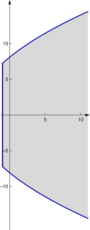 (a) , ,
 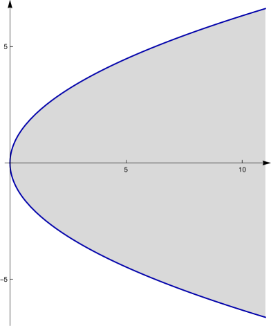 (b) ,
(b) ,
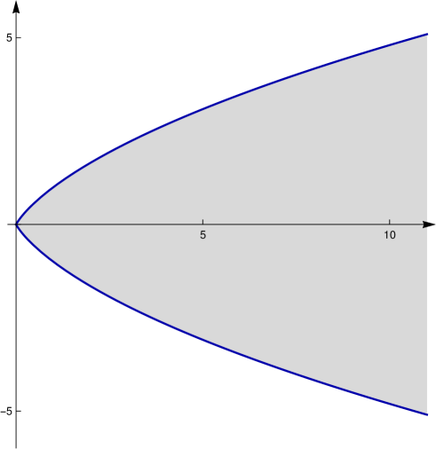 (c) ,
(c) , 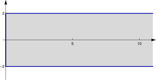 (d) ,
(d) , 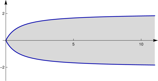 (e) ,
(e) ,