*[subfigure]position=bottom

Spectral gaps and discrete magnetic Laplacians

John Stewart Fabila-Carrasco Department of Mathematics, University Carlos III de Madrid, Avda. de la Universidad 30, 28911. Legan s (Madrid), Spain. jfabila@math.uc3m.es , Fernando Lledó Department of Mathematics, University Carlos III de Madrid, Avda. de la Universidad 30, 28911. Legan s (Madrid), Spain and Instituto de Ciencias Matem ticas (CSIC-UAM-UC3M-UCM), Madrid. flledo@math.uc3m.es and Olaf Post Fachbereich 4 – Mathematik, Universität Trier, 54286 Trier, Germany olaf.post@uni-trier.de

Abstract.

The aim of this article is to give a simple geometric condition that guarantees the existence of spectral gaps of the discrete Laplacian on periodic graphs. For proving this, we analyse the discrete magnetic Laplacian (DML) on the finite quotient and interpret the vector potential as a Floquet parameter. We develop a procedure of virtualising edges and vertices that produces matrices whose eigenvalues (written in ascending order and counting multiplicities) specify the bracketing intervals where the spectrum of the Laplacian is localised. We prove Higuchi-Shirai’s conjecture for $\mathbb{Z}$ -periodic trees and apply our technique in several examples like the polypropylene or the polyacetylene to show the existence of spectral gaps.

Key words and phrases:

Discrete magnetic Laplacian, spectral gaps on periodic graphs, Laplacian on graphs, spectral ordering

2010 Mathematics Subject Classification:

05C50, 47B39, 47A10, 05C65

JSFC was supported by Spanish Ministry of Economy and Competitiveness through project DGI MTM2014-54692-P

FLl was supported by Spanish Ministry of Economy and Competitiveness through project DGI MTM2014-54692-P and the Severo Ochoa Program for Centers of Excellence in R&D (SEV-2015-0554).

OP acknowleges support from the EPSRC funded research network “Analysis on Graphs”.

1. Introduction

The analysis of Schrödinger operators (in particular Laplacians) and their spectra on periodic structures is one of the most important features in solid state physics. Periodicity here means that there is a discrete group $\Gamma$ (typically Abelian) acting on the underlying structure, e.g., a manifold or a graph, with compact quotient that commutes with the operator. Using Floquet theory, the analysis of the operator can be reduced to the analysis of a related family of operators on the quotient. In the case of graphs, the family of operators corresponds to a family of finite dimensional operators, i.e., matrices.

Let $\widetilde{\mathbf{G}}$ be a $\Gamma$ -periodic discrete graph with quotient graph $\mathbf{G}$ . The aim of the present article is to present simple geometric conditions on $\mathbf{G}$ that imply that the Laplacian $\Delta^{\widetilde{\mathbf{G}}}$ (with standard, combinatorial or general periodic weights) on the infinite periodic graph $\widetilde{\mathbf{G}}$ has not the maximal possible interval as spectrum. Such Laplacians are said to have a spectral gap. To show the existence of spectral gaps we develop a purely discrete bracketing technique based on virtualisation of edges and vertices on $\mathbf{G}$ for the discrete magnetic Laplacian on $\mathbf{G}$ . In the context of periodic manifolds or metric graphs Dirichlet-Neumann bracketing allows to localise the spectrum of the differential operator in certain closed intervals whose end points are specified by the Laplacian on a fundamental domain with Dirichlet or Neumann boundary conditions (see, e.g., [LP08a, LP08b, LP07] and references cited therein). Our method of virtualisation of edges and vertices can be seen as a discrete version of Dirichlet-Neumann bracketing.

An important ingredient of our analysis is the discrete magnetic Laplacian (DML). It is a natural generalisation of the usual Laplacian and incorporates the presence of a magnetic field on the graph. Typically the magnetic field enters in the analysis via a vector potential, which is a function of the edges $\alpha\colon E\to\mathbb{R}/2\pi\mathbb{Z}$ . Discrete magnetic Laplacians on covering graphs with general discrete group actions have already been treated, e.g., in [Sun94] and [MY02, MSY03], also for general periodic magnetic fields. Magnetic Laplacians and Laplacians on Abelian covering graphs are discussed also in [HS99, HS04]. Korotyaev and Saburova treated discrete Schrödinger operators on discrete graphs in a series of articles (see, e.g., [KS14, KS15, KS17] and references therein).

In [KS15] the authors develop a bracketing technique similar to the Dirichlet-Neumann bracketing mentioned before and proved estimates of the position of the spectral bands for the combinatorial Laplacian in terms of suitable Neumann and Dirichlet eigenvalue intervals. Moreover, they give an upper estimate of the total band length in terms of these eigenvalues and some geometric data of the graph; this method is extended in [KS17] to the case of magnetic Laplacians with periodic magnetic vector potentials. A method to open gaps in the spectrum — completely independent of the periodicity of the underlying graph — was presented by Schenker and Aizenman in [AS00], decorating each vertex of the original graph with a copy of a given finite graph.

Periodic graphs can also be understood as covering graphs (see, e.g., [Sun08, Sun13]). The existence of spectral gaps is related with the full spectrum conjecture stating that the discrete Laplacian on a maximal Abelian covering $\pi\colon\widetilde{\mathbf{G}}\to\mathbf{G}=\widetilde{\mathbf{G}}/\Gamma$ has maximal possible spectrum. A covering is maximal Abelian if the covering group is $\Gamma=\mathbb{Z}^{b}$ , where $b=b(\mathbf{G})=|V(\mathbf{G})|-|E(\mathbf{G})|+1$ is the first Betti number of $\mathbf{G}$ (see [Sun13, Chapter 6] for details; as usual $V(\mathbf{G})$ and $E(\mathbf{G})$ denote the set of vertices and edges of $\mathbf{G}$ , respectively). The conjecture states that the (standard) Laplacian on a maximal Abelian covering has maximal possible spectrum $[0,2]$ , i.e., no spectral gaps (see [HS99, Conjecture 3.5]) — at least when there is no vertex of degree $1$ . This conjecture was partially solved by [HS99, Proposition 3.6 and 3.8] for graphs where all vertices have even degrees, and certain regular graphs with odd degrees. Graphs with even vertex degrees allow so-called Euler paths, related to the famous Königsberg bridges problem due to Euler. In addition, Higuchi and Shirai [HS04] also realised that one needs additional conditions for the conjecture to be true; namely that there is no vertex of degree $1$ . We confirm this conjecture for periodic trees (i.e., when the quotient graph has Betti number $1$ ). Moreover, Higuchi and Nomura [HN09] show that the normalised Laplacian on a maximal Abelian covering graph of a finite even-regular graph respectively odd-regular and bipartite graph has absolutely continuous spectrum and no eigenvalues.

The article is structured as follows: in Section 2 we recall basic definitions and results on discrete weighted graphs and DMLs. The use of weighted graphs is particularly well adapted to the virtualisation procedure described below, since, for example, the virtualisation of an edge $e$ can also be understood by changing the edge weight to $m_{e}=0$ . In Section 3 we develop a discrete bracketing technique for finite weighted graphs which is based on the manipulation of the (finite) fundamental domain of the periodic discrete graph. This technique is based on a selective virtualisation of certain edges $E_{0}\subset E$ and vertices $V_{0}\subset V$ of a given weighted graph $\mathbf{W}=(\mathbf{G},m)$ with vector potential $\alpha$ and weights $m$ on $V$ and $E$ , respectively. The process of edge and vertex virtualisation produces two different graphs $\mathbf{W}^{-}=(\mathbf{G}^{-},m^{-})$ respectively $\mathbf{W}^{+}=(\mathbf{G}^{+},m^{+})$ with induced vector potentials and weights, such that the spectra of the corresponding DMLs have the following relation:

\lambda_{k}(\Delta_{\alpha^{-}}^{\mathbf{W}^{-}})\leq\lambda_{k}(\Delta_{\alpha}^{\mathbf{W}})\leq\lambda_{k}(\Delta_{\alpha^{+}}^{\mathbf{W}^{+}}),\quad k=1,\dots,n-r,

where $n=|V(\mathbf{G})|$ and $r$ is the number of virtualised vertices. We then say that $\Delta^{\mathbf{W}^{-}}_{\alpha^{-}}$ is spectrally smaller than $\Delta_{\alpha}^{\mathbf{W}}$ (resp. $\Delta_{\alpha}^{\mathbf{W}}$ is spectrally smaller than $\Delta_{\alpha^{+}}^{\mathbf{W}^{+}}$ ) and write

\Delta^{\mathbf{W}^{-}}_{\alpha^{-}}\preccurlyeq\Delta_{\alpha}^{\mathbf{W}}\preccurlyeq\Delta_{\alpha^{+}}^{\mathbf{W}^{+}}.

Virtualising the edges $E_{0}$ on which the vector potential is supported and a corresponding set of vertices $V_{0}$ in the neighbourhood of $E_{0}$ (see Section 3 for precise definitions) we are able to make the DMLs on $\mathbf{G}^{\pm}$ independent of the vector potential $\alpha$ . Hence, also the bracketing intervals

J_{k}:=[\lambda_{k}(\Delta^{\mathbf{W}^{-}}),\lambda_{k}(\Delta^{\mathbf{W}^{+}})]

in which we are going to localise later the spectrum of the periodic infinite Laplacian, are independent of the vector potential.

Theorem (cf., Theorem 3.14).

Let $\mathbf{W}=(\mathbf{G},m)$ be a finite weighted graph and $E_{0}\subset E(\mathbf{G})$ . Then for any vector potential $\alpha$ supported in $E_{0}$ and any vertex set $V_{0}$ in the neighbourhood of $E_{0}$ we have

\Delta^{\mathbf{W}^{-}}\preccurlyeq\Delta^{\mathbf{W}}_{\alpha}\preccurlyeq\Delta^{\mathbf{W}^{+}},

(1.1)

where $\mathbf{W}^{-}=(\mathbf{G}^{-},m^{-})$ with $\mathbf{G}^{-}=\mathbf{G}-E_{0}$ and $\mathbf{W}^{+}=(\mathbf{G}^{+},m^{+})$ with $\mathbf{G}^{+}=\mathbf{G}-V_{0}$ . In particular, we have the spectral localising inclusion

\sigma(\Delta^{\mathbf{W}}_{\alpha})\subset J:=J(\Delta^{\mathbf{W}^{-}},\Delta^{\mathbf{W}^{+}})=\bigcup_{k=1}^{|V(\mathbf{G})|}\bigl{[}\lambda_{k}(\Delta^{\mathbf{W}^{-}}),\lambda_{k}(\Delta^{\mathbf{W}^{+}})\bigr{]}.

(1.2)

In Section 4 we introduce the notion of magnetic spectral gaps set which in the case of standard weights is given by

\mathcal{MS}^{\mathbf{W}}=[0,2]\setminus\bigcup_{\alpha\in\mathcal{A}(\mathbf{G})}\sigma(\Delta^{\mathbf{W}}_{\alpha}),

where $\mathcal{A}(\mathbf{G})$ denotes the set of all vector potentials on $\mathbf{G}$ . In other words, the magnetic spectral gap set is the intersection of all resolvent sets of the DML $\Delta^{\mathbf{W}}_{\alpha}$ for all $\alpha\in\mathcal{A}(\mathbf{G})$ , with the set $[0,2]$ . If $\mathbf{G}$ is a tree then $\mathcal{MS}^{\mathbf{W}}$ coincides with the spectral gaps set $\mathcal{S}^{\mathbf{W}}$ of the usual Laplacian $\Delta^{\mathbf{W}}$ with $\alpha=0$ . In Theorem 4.4 we give a sufficient geometrical condition on the weighted graph such that the set of magnetic spectral gaps is non-empty. As a consequence of this result we give several characterisations of $\mathcal{MS}^{\mathbf{W}}\not=\emptyset$ for finite weighted graphs with Betti number $1$ (cf., Corollary 4.7). We also present here several examples of finite graphs with nonempty magnetic spectral gaps set and show spectral localisation of the spectrum of the DMLs in the bracketing intervals.

In Section 5 we introduce first basic notation and results on $\Gamma$ -periodic graphs $\widetilde{\mathbf{G}}$ with finite quotient $\mathbf{G}=\widetilde{\mathbf{G}}/\Gamma$ and Abelian discrete group $\Gamma$ . In particular, we remind a discrete version of Floquet theory and interpret the vector potential $\alpha$ on $\mathbf{G}$ as a Floquet parameter. Applying then results of the previous sections to the finite quotient we prove of Higuchi-Shirai’s conjecture for $\mathbb{Z}$ -periodic trees, i.e., we prove the following result:

Theorem (cf., Theorem 5.8).

Let $\widetilde{\mathbf{W}}=(\widetilde{\mathbf{G}},\widetilde{m})$ be a $\mathbb{Z}$ -periodic tree with standard or combinatorial weights and quotient graph $\mathbf{W}=(\mathbf{G},m)$ . Then the following conditions are equivalent:

(a)

$\widetilde{\mathbf{W}}$ has the full spectrum property;
(b)

$\mathcal{S}^{\widetilde{\mathbf{W}}}=\emptyset$ ;
(c)

$\widetilde{\mathbf{W}}$ is the lattice $\mathbb{Z}$ ;
(d)

$\mathcal{MS}^{\mathbf{W}}=\emptyset$ ;
(e)

$\mathbf{G}$ is a cycle graph;
(f)

$\mathbf{G}$ has no vertex of degree $1$ .

Finally, we also apply the bracketing method to show that the spectrum of the Laplacian $\Delta^{\widetilde{\mathbf{G}}}$ is localised in the union of the bracketing intervals. This gives a sufficient condition for the existence of spectral gaps in the spectrum of $\Delta^{\widetilde{\mathbf{G}}}$ .

In Section 6 we apply the methods developed to several classes of examples of periodic graphs. The first example gives simple verification of results by Suzuki in [Suz13] on the existence of spectral gaps for $\mathbb{Z}$ -periodic graphs with pendants. The other examples are more elaborate and include modelisations of polypropylene and polyacetylene molecules. We prove also the existence of spectral gaps in these periodic structures. The last example can be understood as an intermediate covering of the graphene where the quotient has Betti number $2$ .

Notation

We denote a weighted graph by $\mathbf{W}=(\mathbf{G},m)$ where $\mathbf{G}=(V,E,\partial)$ is an oriented graph and $m$ a weight on the vertices $V$ and edges $E$ . For a vector potential $\alpha$ , the operator $\Delta_{\alpha}^{\mathbf{G}}$ denotes the discrete magnetic Laplacian (DML) with standard weights and $\Delta_{\alpha}^{\mathbf{W}}$ corresponds to the DML to denote a generic weighted graph. We use $\Delta^{\mathbf{G}}$ , $\mathcal{MS}^{\mathbf{G}}$ and $\mathcal{S}^{\mathbf{G}}$ to denote the usual Laplacian, the set of magnetic spectral gaps and the set of spectral gaps with standard weights, respectively, and $\Delta^{\mathbf{W}}$ , $\mathcal{MS}^{\mathbf{W}}$ and $\mathcal{S}^{\mathbf{W}}$ for the corresponding objects with generic weights. We denote $\widetilde{\mathbf{W}}=(\widetilde{\mathbf{G}},\widetilde{m})$ a periodic weighted graph.

Acknowledgements

We would like to thank Pavel Exner for encouraging us to extend the previous article on bracketing techniques in [LP08a] also to magnetic Laplacians. We would also like to thank the anonymous referee for carefully reading our manuscript and for his useful suggestions.

2. Discrete graphs and discrete magnetic Laplacians

In this section we introduce the necessary background on discrete graphs and Laplacians that will be used later.

2.1. Graphs and subgraphs

In this article $\mathbf{G}=(V,E,\partial)$ denotes a (discrete) directed graph, i.e., $V=V(\mathbf{G})$ is the set of vertices, $E=E(\mathbf{G})$ the set of edges and $\partial\colon E\rightarrow V\times V$ is the orientation map. Here, $\partial e=(\partial_{-}e,\partial_{+}e)$ denotes the pair of the initial and terminal vertices. We allow graphs with multiple edges, i.e., edges $e_{1}\neq e_{2}$ with $(\partial_{-}e_{1},\partial_{+}e_{1})=(\partial_{-}e_{2},\partial_{+}e_{2})$ or $(\partial_{-}e_{1},\partial_{+}e_{1})=(\partial_{+}e_{2},\partial_{-}e_{2})$ and loops, i.e., edges $e_{1}$ with $\partial_{-}{e_{1}}=\partial_{+}{e_{1}}$ . We define

E_{v}:=E_{v}^{+}\operatorname*{\mathaccent 0{\cdot}\cup}E_{v}^{-}\quad\text{(disjoint union), where}\quad E^{\pm}_{v}:=\{e\in E\mid v=\partial_{\pm}e\}\;.

The degree of a vertex is $\deg(v)=|E_{v}|$ ; note that, since $E_{v}$ is defined in terms of a disjoint union, a loop increases the degree by $2$ .

For subsets $A,B\subset V$ , denote by

E^{+}(A,B):=\{e\in E\mid\partial_{-}e\in A,\partial_{+}e\in B\}\quad\text{and}\quad E^{-}(A,B):=E^{+}(B,A).

In particular, $E^{\pm}_{v}=E^{\pm}(V,\{v\})$ . Moreover, we set

E(A,B):=E^{+}(A,B)\cup E^{-}(A,B)\qquad\text{and}\qquad E(A):=E(A,A).

To simplify the notation, we write $E(v,w)$ instead of $E(\{v\},\{w\})$ etc. Note that loops are not counted double in $E(A,B)$ , in particular, $E(v):=E(v,v)$ is the set of loops based at the vertex $v\in V$ . The Betti number $b(\mathbf{G})$ of a finite graph $\mathbf{G}=(V,E,\partial)$ is defined as

b(\mathbf{G}):=|E|-|V|+1.

(2.1)

When we analyse in the next sections virtualisation processes of vertices, edges and fundamental domains in periodic graphs, it will be convenient to consider the following substructure of a graph.

Definition 2.1.

Let $\mathbf{G}=(V,E,\partial)$ be a discrete graph and $\mathbf{H}=(V_{0},E_{0},\partial_{0})$ be a triple such that $V_{0}\subset V$ , $E_{0}\subset E$ and $\partial_{0}=\partial\restriction_{E_{0}}$ .

(a)

If $E_{0}\cap E(V\setminus V_{0})=\emptyset$ , we say that $\mathbf{H}$ is a partial subgraph in $\mathbf{G}$ . We call

	$\displaystyle B(\mathbf{H},\mathbf{G}):=$	$\displaystyle E(V_{0},V\setminus V_{0})$
	$\displaystyle=$	$\displaystyle\{e\in E\mid\partial_{-}e\in V_{0},\partial_{+}e\in V\setminus V_{0}\text{ or }\partial_{+}e\in V_{0},\partial_{-}e\in V\setminus V_{0}\}$		(2.2)

the set of connecting edges of the partial subgraph $\mathbf{H}$ in $\mathbf{G}$ .

(b)

If $E_{0}\subset E(V_{0})$ , we say that $\mathbf{H}$ is a subgraph of $\mathbf{G}$ .
(c)

If $E_{0}=E(V_{0})$ , we say that $\mathbf{H}$ is an induced subgraph of $\mathbf{G}$ .
(d)

If $\mathbf{H}$ is a subgraph of $\mathbf{G}$ with $V_{0}=V(\mathbf{G})$ such that $\mathbf{H}$ is connected and has no cycles, we say that $\mathbf{H}$ is an induced tree of $\mathbf{G}$ .

Remark 2.2.

(a)

Note that a partial subgraph $\mathbf{H}=(V_{0},E_{0},\partial_{0})$ is not a graph as defined in Section 2.1, since we do not exclude edges $e\in E$ with $\partial_{\pm}e\notin V_{0}$ ; we only exclude the case that $\partial_{+}e\notin V_{0}$ and $\partial_{-}e\notin V_{0}$ . The edges not mapped into $V_{0}\times V_{0}$ under $\partial_{0}$ are precisely the connecting edges of $\mathbf{H}$ in $\mathbf{G}$ . In other words, we only have $\partial_{0}\colon B(\mathbf{H},\mathbf{G})\rightarrow V\times V$ , but $\partial_{0}\colon E_{0}\setminus B(\mathbf{H},\mathbf{G})\rightarrow V_{0}\times V_{0}$ .
(b)

In contrast, for a subgraph or an induced subgraph, $\mathbf{H}$ is itself a discrete graph as $E_{0}\subset E(V_{0})$ and hence $\partial_{0}$ maps $E_{0}$ into $V_{0}\times V_{0}$ . Moreover, a subgraph (or an induced subgraph) has no connecting edges in $\mathbf{G}$ .

2.2. Weighted discrete graphs

Let $\mathbf{G}=(V,E,\partial)$ be a discrete graph. A weight on $\mathbf{G}$ is a pair of functions $m$ on the vertices and edges $m\colon V\rightarrow(0,\infty)$ and $m\colon E\rightarrow(0,\infty)$ associating to a vertex $v$ its weight $m(v)$ and to an edge $e$ its weight $m_{e}$ .¹¹1Later, the virtualization process of edges can also be interpreted allowing $m_{e}=0$ on certain edges $e$ .

We call $\mathbf{W}=(\mathbf{G},m)$ a weighted discrete graph. Now, it is natural to define $m(E_{0})=\sum_{e\in E_{0}}m_{e}$ for any $E_{0}\subset E$ . The relative weight is $\rho\colon V\rightarrow(0,\infty)$ defined as

	$\rho(v):=\dfrac{m(E_{v})}{m(v)}=\dfrac{m(E_{v}^{+})+m(E_{v}^{-})}{m(v)}.$	(2.3a)
If we need to stress the dependence of $\rho$ of the weighted graph, we simply write $\rho^{\mathbf{W}}$ . We will assume throughout this article that the relative weight is uniformly bounded, i.e.,
	$\rho_{\infty}:=\sup_{v\in V}\rho(v)<\infty.$	(2.3b)

This condition will ensure later on that the discrete magnetic Laplacian is a bounded operator.

Examples of commonly used weights are the following:

Weight name	$m_{e}$	$m(v)$	$\rho(v)$	$\rho_{\infty}$
standard	$1$	$\deg v$	$1$	$1$
combinatorial	$1$	$1$	$\deg v$	$\sup_{v\in V}\deg v$
normalised	$m_{e}$	$m(E_{v})$	$1$	$1$
electric circuit	$m_{e}$	$1$	$m(E_{v})$	$\sup_{v\in V}m(E_{v})$

Note that the first two weights are intrinsic, i.e., they can be calculated just by the graph data, while the last two need the additional information of an edge weight $m\colon E\to(0,\infty)$ .

To a weighted graph $\mathbf{W}=(\mathbf{G},m)$ we associate the following two Hilbert spaces

	$\displaystyle\ell_{2}(V,m)$	$\displaystyle:=\Bigl{\{}f\colon V\rightarrow\mathbb{C}\mid\left\\|f\right\\|_{V,m}^{2}=\sum_{v\in V}\|f(v)\|^{2}m(v)<\infty\Bigr{\}}\qquad\text{and}$
	$\displaystyle\ell_{2}(E,m)$	$\displaystyle:=\Bigl{\{}\eta\colon E\rightarrow\mathbb{C}\mid\left\\|\eta\right\\|_{E,m}^{2}=\sum_{e\in E}\|\eta_{e}\|^{2}m_{e}<\infty\Bigr{\}},$

with inner products

\left\langle f,g\right\rangle_{\ell_{2}(V,m)}=\sum_{v\in V}{f(v)}\overline{g(v)}m(v)\quad\text{and}\quad\left\langle\eta,\zeta\right\rangle_{\ell_{2}(E,m)}=\sum_{e\in E}\eta_{e}\overline{\zeta_{e}}m_{e},

respectively. These spaces can be interpreted as $0$ - and $1$ -forms on the graph, respectively.

2.3. Discrete magnetic Laplacian

Let $\mathbf{W}=(\mathbf{G},m)$ a weighted graph. A vector potential $\alpha$ acting on $\mathbf{G}$ is a $\mathbb{T}$ -valued function on the edges as follows, $\alpha\colon E(\mathbf{G})\rightarrow\mathbb{T}=\mathbb{R}/2\pi\mathbb{Z}.$ We denote the set of all vector potentials on $E(\mathbf{G})$ just by $\mathcal{A}(\mathbf{G})$ . We say that two vector potentials $\alpha_{1}$ and $\alpha_{2}$ are cohomologous, and denote this as $\alpha_{1}\sim\alpha_{2}$ , if there is $\varphi\colon V\rightarrow\mathbb{T}$ with

\alpha_{1}=\alpha_{2}+d\varphi.

Given a $E_{0}\subset E(\mathbf{G})$ , we say that a vector potential $\alpha$ has support in $E_{0}$ if $\alpha_{e}=0$ for all $e\in E(\mathbf{G})\setminus E_{0}$ .

It can be shown that any vector potential on a finite graph can be supported in $b(\mathbf{G})$ many edges. In fact, let $\mathbf{G}$ a finite graph with $\alpha$ a vector potential acting on it and let $\mathbf{T}$ an induced tree of $\mathbf{G}$ . Then we can show that there exists a vector potential $\alpha^{\prime}$ with support in $E(\mathbf{G})\setminus E(\mathbf{T})$ such that $\alpha\sim\alpha^{\prime}$ . In particular, if $\mathbf{G}$ is a cycle, any vector potential is cohomologous to a vector potential supported in only one edge. Moreover, if $\mathbf{G}$ is a tree any vector potential on a tree is cohomologous to $0$ .

The twisted (discrete) derivative is the operator between $0$ -forms and $1$ -forms given by

d_{\alpha}\colon\ell_{2}(V,m)\rightarrow\ell_{2}(E,m)\qquad\text{with}\qquad\left(d_{\alpha}f\right)_{e}=\mathrm{e}^{\mathrm{i}\alpha_{e}/2}f(\partial_{+}e)-\mathrm{e}^{-\mathrm{i}\alpha_{e}/2}f(\partial_{-}e).

(2.4)

Definition 2.3.

Let $\mathbf{W}=(\mathbf{G},m)$ be a weighted graph with $\alpha$ a vector potential. The discrete magnetic Laplacian (DML) $\Delta_{\alpha}\colon\ell_{2}(V)\rightarrow\ell_{2}(V)$ is defined by $\Delta_{\alpha}=d_{\alpha}^{*}d_{\alpha}$ , i.e., by

\left(\Delta_{\alpha}f\right)\left(v\right)=\rho(v)f(v)-\dfrac{1}{m(v)}\sum_{e\in E_{v}}{\mathrm{e}^{\mathrm{i}\accentset{\curvearrowright}{\alpha}_{e}(v)}}f(v_{e})m_{e},

where $\accentset{\curvearrowright}{\alpha}_{e}(v)$ resp. $v_{e}$ is the oriented evaluation resp. opposite vertex of $v$ along the edge $e$ , i.e.,

\accentset{\curvearrowright}{\alpha}_{e}(v)=\begin{cases}-\alpha_{e},&\text{if $v=\partial_{-}e$,}\\ \alpha_{e},&\text{if $v=\partial_{+}e$,}\end{cases}\quad\text{resp.}\quad v_{e}=\begin{cases}\partial_{+}e,&\text{if $v=\partial_{-}e$,}\\ \partial_{-}e&\text{if $v=\partial_{+}e$.}\end{cases}

If we need to stress the dependence on the weighted graph $\mathbf{W}=(\mathbf{G},m)$ we will denote the DML as $\Delta_{\alpha}^{\mathbf{W}}$ .

The DML $\Delta_{\alpha}$ is a bounded, positive and self-adjoint operator and its spectrum satisfies $\sigma(\Delta_{\alpha})\subset[0,2\rho_{\infty}]$ . Unlike the usual Laplacian without magnetic potential, the DML does depend on the orientation of the graph. If $\alpha\sim\alpha^{\prime}$ , then $\Delta_{\alpha}$ and $\Delta_{\alpha^{\prime}}$ are unitary equivalent; in particular, $\sigma(\Delta_{\alpha})=\sigma(\Delta_{\alpha^{\prime}})$ . Indeed, if $\alpha^{\prime}=\alpha+d\varphi$ then it is straightforward to check that the unitary operator $(Uf)(v)=\mathrm{e}^{\varphi(v)}f(v)$ intertwines between both DMLs. In particular, if $\alpha\sim 0$ then $\Delta_{\alpha}\cong\Delta$ where $\Delta$ denotes the discrete Laplacian with vector potential $0$ , i.e., the usual discrete Laplacian on $(\mathbf{G},m)$ . For example, if $\mathbf{W}=(\mathbf{G},m)$ with $\mathbf{G}$ being a tree, then $\Delta_{\alpha}^{\mathbf{W}}\cong\Delta^{\mathbf{W}}$ for any vector potential.

If the graph $G=(V,E,\partial)$ is bipartite (i.e., there is a partition $V=A\operatorname*{\mathaccent 0{\cdot}\cup}B$ such that $E=E(A,B)$ , we have the following spectral symmetry (see, e.g., [LP08b, Prp. 2.3]):

Proposition 2.4.

Assume that $\mathbf{W}=(\mathbf{G},m)$ is a weighted graph with bipartite graph $\mathbf{G}$ and normalised weight $m$ . Then the spectrum of $\Delta^{\mathbf{W}}$ (with vector potential $\alpha=0$ ) is symmetric with respect to the map $\kappa\colon\mathbb{R}\to\mathbb{R}$ , $\kappa(\lambda)=2-\lambda$ , i.e.,

\kappa(\sigma(\Delta^{\mathbf{W}}))=\sigma(\Delta^{\mathbf{W}}).

In particular, if $J\subset[0,2]$ fulfils $\sigma(\Delta^{\mathbf{W}})\subset J$ , then we have the inclusion

\sigma(\Delta^{\mathbf{W}})\subset J\cap\kappa(J).

Note that the set $J\cap\kappa(J)$ becomes smaller than $J$ if $J$ is not symmetric with respect to $\kappa$ .

2.4. Matrix representation of the DML

For computing the eigenvalues of the DML it is convenient to work with the associated matrix. Given a finite weighted graph $(\mathbf{G},m)$ with vector potential $\alpha$ . Consider a numbering of the vertices as $V(\mathbf{G})=\left\{v_{1},v_{2},\dots,v_{n}\right\}$ . Then $\left\{\varphi_{v_{i}}\right\}_{i=1}^{n}\subset\ell_{2}(V,m)$ with $\varphi_{v_{i}}=m(v_{i})^{-1/2}\mathbbm{1}_{\left\{v_{i}\right\}}$ is an orthonormal basis of $\ell_{2}(V,m)$ . The matrix representation of $\Delta_{\alpha}$ with respect to this orthonormal basis is given by

\left[\Delta_{\alpha}\right]_{jk}=\begin{cases}\displaystyle\rho(v_{j})-\frac{1}{m(v_{j})}\sum_{e\in E(v_{j},v_{j})}\Bigl{(}\underbrace{\mathrm{e}^{\mathrm{i}\alpha_{e}}+\mathrm{e}^{-\mathrm{i}\alpha_{e}}}_{=2\cos\alpha_{e}}\Bigr{)}m_{e},&\text{if $j=k$,}\\[8.61108pt] \displaystyle-\frac{1}{\sqrt{m(v_{j})m(v_{k})}}\Bigl{(}\sum_{e\in E^{+}(v_{j},v_{k})}\mathrm{e}^{\mathrm{i}\alpha_{e}}m_{e}+\sum_{e\in E^{-}(v_{j},v_{k})}\mathrm{e}^{-\mathrm{i}\alpha_{e}}m_{e}\Bigr{)},&\text{if $v_{j}\sim v_{k}$,}\\[8.61108pt] 0&\text{otherwise.}\end{cases}

where $v_{j}\sim v_{k}$ meaning that $v_{j}$ and $v_{k}$ are connected by an edge. Note that this formula includes the case of graphs with multiple edges and loops.

3. Spectral ordering on finite graphs

In this section we will introduce one spectral ordering and two operation on the graphs that will be needed later to develop a discrete bracketing technique and show the existence of spectral gaps for Laplacians on periodic graphs. Korotyaev and Saburova also present a discrete bracketing technique in [KS15] for combinatorial weights. Their Dirichlet upper bound of the bracketing is similar to the one we use here (vertex-virtualised). For the lower bound Korotyaev and Saburova use a Neumann type boundary condition while we propose an alternative edge virtualization process using the fact that we work with arbitrary weights. In our approach the virtualisation is done is such a way that vector potential on the resulting graphs (deleting edges and deleting vertices) is cohomologous to zero.

Let $\mathbf{W}=(\mathbf{G},m)$ a weighted graph. Throughout this section, we will assume that $|V(\mathbf{G})|<\infty$ . If $|V(\mathbf{G})|=n$ , then we denote the spectrum of the DML by $\sigma(\Delta^{\mathbf{W}}_{\alpha}):=\{\lambda_{k}(\Delta^{\mathbf{W}}_{\alpha})\mid k=1,\dots,n\}$ , where we will write the eigenvalues in ascending order and repeated according to their multiplicities, i.e.,

0\leq\lambda_{1}(\Delta^{\mathbf{W}}_{\alpha})\leq\lambda_{2}(\Delta^{\mathbf{W}}_{\alpha})\leq\cdots\leq\lambda_{n}(\Delta^{\mathbf{W}}_{\alpha}).

Definition 3.1.

Let $S^{-}$ and $S^{+}$ be self-adjoint operators on $n^{-}$ - respectively $n^{+}$ -dimensional Hilbert spaces and consider the eigenvalues written in ascending order and repeated according to their multiplicities. We say that $S^{-}$ is spectrally smaller than $S^{+}$ (denoted by $S^{-}\preccurlyeq S^{+}$ ), if

n^{-}\geq n^{+}\qquad\text{and if}\qquad\lambda_{k}(S^{-})\leq\lambda_{k}(S^{+})\quad\text{for all}\quad 1\leq k\leq n^{+}.

Assume now that all operators have spectrum (i.e., eigenvalues) in $[0,2\rho_{\infty}]$ for some number $\rho_{\infty}>0$ . If we set $\lambda_{k}(S^{+})=2\rho_{\infty}$ for $k=n^{+}+1,\dots,n^{-}$ (the maximal possible eigenvalue), then we can replace the eigenvalue estimate in the previous definition by

\lambda_{k}(S^{-})\leq\lambda_{k}(S^{+})\quad\text{for all}\quad 1\leq k\leq n^{-}.

Note also that the relation $\preccurlyeq$ is invariant under unitary conjugation of the operator.

Definition 3.2.

For operators $S^{-}$ and $S^{+}$ with $S^{-}\preccurlyeq S^{+}$ we define the associated $k$ -th bracketing interval $J_{k}=J_{k}(S^{-},S^{+})$ by

J_{k}:=\bigl{[}\lambda_{k}(S^{-}),\lambda_{k}(S^{+})\bigr{]}

(3.1)

for $k=1,\dots,n^{-}$ .

If now $T$ is an operator with $S^{-}\preccurlyeq T\preccurlyeq S^{+}$ , then we have the following eigenvalue bracketing

\lambda_{k}(T)\in J_{k}

(3.2)

for all $k=1,\dots,n^{-}$ . Moreover,

\sigma(T)\subset J:=\bigcup_{k=1}^{n^{-}}J_{k}

(3.3)

and we call $J=J(S^{-},S^{+})$ the spectral localising set of the pair $S^{-}$ and $S^{+}$ .

The key observation for detecting spectral gaps from the eigenvalue bracketing is the following:

Proposition 3.3.

Let $S^{-}$ and $S^{+}$ be operators on $n^{-}$ , respectively $n^{+}$ , finite dimensional Hilbert spaces with spectrum in $[0,2\rho_{\infty}]$ . Let $\mathcal{T}$ be a subset of the set of operators $T$ on a finite dimensional Hilbert spaces with $S^{-}\preccurlyeq T\preccurlyeq S^{+}$ , then

\mu\Bigl{(}\bigcup_{T\in\mathcal{T}}\sigma(T)\Bigr{)}\leq\operatorname{Tr}(S^{+})-\operatorname{Tr}(S^{-})+2\rho_{\infty}(n^{-}-n^{+})

where $\mu$ denotes the $1$ -dimensional Lebesgue measure. In particular, if $n^{-}-n^{+}=1$ and $\operatorname{Tr}(S^{+})-\operatorname{Tr}(S^{-})<0$ , then $\bigcup_{T\in\mathcal{T}}\sigma(T)$ cannot be the entire interval $[0,2\rho_{\infty}]$ .

Proof.

We have

\mu\Bigl{(}\bigcup_{T\in\mathcal{T}}\sigma(T)\Bigr{)}\leq\mu\Bigl{(}\bigcup_{k=1}^{n^{-}}J_{k}\Bigr{)}\leq\sum_{k=1}^{n^{-}}\bigl{(}\lambda_{k}(S^{+})-\lambda_{k}(S^{-}))=\operatorname{Tr}(S^{+})+2\rho_{\infty}(n^{-}-n^{+})-\operatorname{Tr}(S^{-}).\qed

We begin with the description of a procedure of manipulation of the graph that will lead to a spectrally smaller DML.

Definition 3.4 (virtualising edges).

Let $\mathbf{W}=(\mathbf{G},m)$ be a weighted graph with vector potential $\alpha$ and $E_{0}\subset E(\mathbf{G})$ . We denote by $\mathbf{W}^{-}=(\mathbf{G}^{-},m^{-})$ the weighted subgraph with vector potential $\alpha^{-}$ defined as follows:

(a)

$V(\mathbf{G}^{-})=V(\mathbf{G})$ with $m^{-}(v):=m(v)$ for all $v\in V(\mathbf{G})$ ;
(b)

$E(\mathbf{G}^{-})=E(\mathbf{G})\setminus E_{0}$ with $m^{-}_{e}:=m_{e}$ and $\partial_{\pm}^{\mathbf{G}^{-}}e=\partial_{\pm}^{\mathbf{G}}e$ for all $e\in E(\mathbf{G}^{-})$ ;
(c)

$\alpha^{-}_{e}=\alpha_{e}$ , $e\in E(\mathbf{G}^{-})$ .

We call $\mathbf{W}^{-}$ the weighted subgraph obtained from $\mathbf{W}$ by virtualising the edges $E_{0}$ . We will sometimes also use the suggestive notation $\mathbf{G}^{-}=\mathbf{G}-E_{0}$ .

The corresponding discrete magnetic Laplacian is denoted by $\Delta_{\alpha^{-}}^{\mathbf{W}^{-}}$ .

Remark 3.5.

(a)

Note that $\Delta_{\alpha^{-}}^{\mathbf{W}^{-}}=(d_{\alpha^{-}})^{*}d_{\alpha^{-}}$ , where $d_{\alpha^{-}}:=\pi\circ d_{\alpha}$ and $\pi\colon\ell_{2}(E(\mathbf{G}),m)\rightarrow\ell_{2}(E(\mathbf{G}^{-}),m^{-})$ is the orthogonal projection onto the functions on the non-virtualised edges. Note that $\pi=\iota^{*}$ with $\iota\colon\ell_{2}(E(\mathbf{G}^{-}),m^{-})\rightarrow\ell_{2}(E(\mathbf{G}),m)$ being the natural inclusion, i.e., for $\eta\in\ell_{2}(E(\mathbf{G}^{-}),m^{-})$ $\iota\eta$ is extended by $0$ on $E(\mathbf{G}^{-})=E(\mathbf{G})\setminus E_{0}$ . Note that the process of virtualisation of edges can be also described by changing the weights on $\mathbf{G}$ : set $m_{e_{0}}=0$ for $e_{0}\in E_{0}$ , and leave all other weights unchanged.
(b)

The process of virtualising edges has consequences for various quantities related to the graph. The most important for us here refers to the spectrum (see the following proposition). If $\rho^{-}$ denotes the relative weight of $\mathbf{W}^{-}$ , then $\rho^{-}(v)\leq\rho(v)$ for $v\in V$ .

Let $\mathbf{W}=(\mathbf{G},m)$ be a weighted graph with standard weights, and denote by $\mathbf{W}^{\prime}=(\mathbf{G}^{-},m^{\prime})$ the graph $\mathbf{G}^{-}$ with standard weights. If $E_{0}\neq\emptyset$ , then there exists a $v\in V(\mathbf{G})$ such that $m^{-}(v)>m^{\prime}(v)$ , i.e., the new weight $m^{-}$ is not standard anymore. More generally, if $\mathbf{W}=(\mathbf{G},m)$ has a normalised weight, then $m^{-}$ is no longer normalised; the relative weights of $\mathbf{W}^{-}$ and $\mathbf{W}^{\prime}$ fulfil $\rho^{-}(v)\leq\rho^{\prime}(v)=1$ with strict inequality for $v\in V(\mathbf{G}^{-})$ incident with an edge in $E_{0}$ .

If $\mathbf{W}=(\mathbf{G},m)$ is a weighted graph with combinatorial weight $m$ , then $m^{-}$ as well has the combinatorial weight , i.e., combinatorial weights are preserved under edge virtualisation.
(c)

It is also clear that if $\mathbf{G}$ is connected, then $\mathbf{G}^{-}$ need not to be connected any more. Moreover, the homology of the graph changes under edge virtualisation. This is perhaps an important motivation of this definition. Later we will exploit the fact that deleting a suitable set of edges the graph will turn it into a tree. The graph $\mathbf{G}^{-}$ is sometimes also called spanning subgraph.

We show next that the process of virtualising edges produces a DML which is spectrally smaller (cf., Definition 3.1).

Proposition 3.6.

Let $\mathbf{W}=(\mathbf{G},m)$ be a weighted graph with vector potential $\alpha$ and $E_{0}\subset E(\mathbf{G})$ . Denote by $\mathbf{W}^{-}=(\mathbf{G}^{-},m^{-})$ with $\mathbf{G}^{-}=\mathbf{G}-E_{0}$ the edge virtualised graph (cf. Definition 3.4), then

\Delta_{\alpha^{-}}^{\mathbf{W}^{-}}\preccurlyeq\Delta_{\alpha}^{\mathbf{W}}.

Proof.

Since $E(\mathbf{G}^{-})\subset E(\mathbf{G})$ we have for $f\in\ell_{2}(V(\mathbf{G}),m)$

\displaystyle\langle{\Delta_{\alpha^{-}}^{\mathbf{W}^{-}}f},{f}\rangle=\|{d_{\alpha^{-}}f}\|^{2}_{\ell_{2}(E(\mathbf{G}^{-}),m^{-})}\leq\|{d_{\alpha}f}\|^{2}_{\ell_{2}(E(\mathbf{G}),m)}=\langle{\Delta_{\alpha}^{\mathbf{W}}f},{f}\rangle\;.

For $k\in\left\{1,2,\dots,|V(\mathbf{G})|\right\}$ denote by $\Xi_{k}$ the set of all intersections $E_{k}$ of $k$ -dimensional subspaces with the $1$ -sphere in $\ell_{2}(V(\mathbf{G}),m)$ . Applying the variational characterisation of the spectrum (see, e.g., [BB92, Theorem 6.1.2]) we conclude

\lambda_{k}(\Delta_{\alpha^{-}}^{\mathbf{W}^{-}})=\min_{E_{k}\in\Xi_{k}}\max_{f\in E_{k}}\|{d_{\alpha^{-}}f}\|^{2}\leq\min_{E_{k}\in\Xi_{k}}\max_{f\in E_{k}}\|{d_{\alpha}f}\|^{2}.

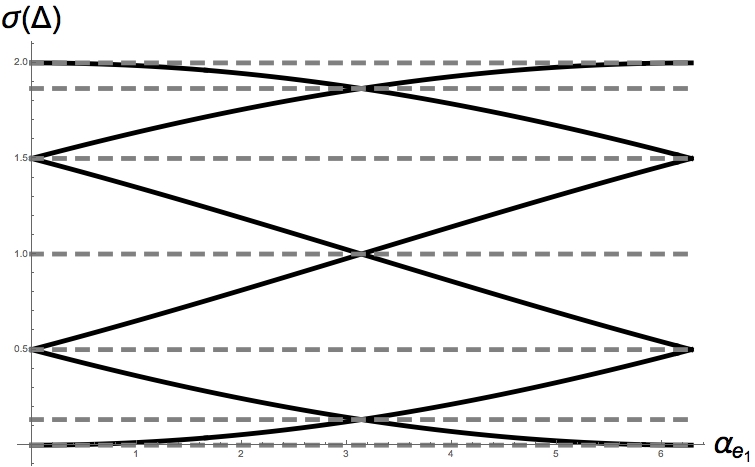
Since $|V(\mathbf{G})|=|V(\mathbf{G}^{-})|$ we have shown $\Delta_{\alpha^{-}}^{\mathbf{W}^{-}}\preccurlyeq\Delta_{\alpha}^{\mathbf{W}}$ . ∎

Example 3.7.

Let $\mathbf{W}=(\mathbf{G},m)$ be the $6$ -cycle with standard weights as in Figure 1. Let $\mathbf{W}^{-}=(\mathbf{G}^{-},m^{-})$ be the graph with the edge $e_{1}$ virtualised (i.e., $\mathbf{G}^{-}=\mathbf{G}-\{e_{1}\}$ , see Definition 3.1, and $m^{-}$ being the restriction of $m$ to $E(\mathbf{G}^{-})=E(\mathbf{G})\setminus\{e_{1}\}$ . If $\alpha$ is any vector potential on $\mathbf{G}$ , then $\alpha$ can be supported on $e_{1}$ , so $\alpha^{-}$ is trivial on $\mathbf{G}^{-}$ . Therefore $\Delta_{\alpha^{-}}^{\mathbf{W}^{-}}$ is unitarily equivalent with $\Delta^{\mathbf{W}^{-}}$ (usual Laplacian with $\alpha=0$ ). Finally, we plot the six eigenvalues of $\Delta_{\alpha}^{\mathbf{G}}$ and $\Delta^{\mathbf{W}^{-}}$ , when $\alpha_{e_{1}}$ runs through $[0,2\pi]$ . This example illustrates $\Delta_{\alpha^{-}}^{\mathbf{W}^{-}}\preccurlyeq\Delta_{\alpha}^{\mathbf{G}}$ hence, by unitary equivalence, also $\Delta^{\mathbf{W}^{-}}\preccurlyeq\Delta_{\alpha}^{\mathbf{G}}$ .

Refer to caption — (a) The graph $\mathbf{G}=C_{6}$ .

Example 3.8.

This example shows that Proposition 3.6 is not true if we insist on having standard weights both in $\mathbf{G}$ and $\mathbf{G}^{-}$ (cf., Remark 3.5 (b)). Take $\mathbf{G}$ and $\mathbf{G}^{-}=C_{6}-\{e_{1}\}$ both with the standard weights. Consider the vector potential supported on $e_{1}$ such that $\alpha_{e_{1}}=\pi/2$ . In this case we have $\lambda_{4}(\Delta^{\mathbf{G}^{-}}_{\alpha^{-}})=\lambda_{4}(\Delta^{\mathbf{G}^{-}})\approx 1.30902\nleq 1.25882\approx\lambda_{4}(\Delta^{\mathbf{G}}_{\alpha})$ , hence $\Delta_{\alpha^{-}}^{\mathbf{G}^{-}}$ is not spectrally smaller than $\Delta_{\alpha}^{\mathbf{G}}$ .

We next describe the second elementary operation on the graph dual to edge virtualising.

Definition 3.9 (virtualising vertices).

Let $\mathbf{W}=(\mathbf{G},m)$ be a weighted graph with vector potential $\alpha$ and $V_{0}\subset V(\mathbf{G})$ . We denote by $\mathbf{W}^{+}=(\mathbf{G}^{+},m^{+})$ the weighted partial subgraph with vector potential $\alpha^{+}$ defined as follows:

(a)

$V(\mathbf{G}^{+})=V(\mathbf{G})\setminus V_{0}$ with $m^{+}(v):=m(v)$ for all $v\in V(\mathbf{G}^{+})$ ;
(b)

$E(\mathbf{G}^{+})=E(\mathbf{G})\setminus E(V_{0})$ with $m^{+}_{e}:=m_{e}$ for all $e\in E(\mathbf{G}^{+})$ ;
(c)

$\alpha^{+}_{e}=\alpha_{e}$ , $e\in E(\mathbf{G}^{+})$ .

We call $\mathbf{W}^{+}$ the weighted partial subgraph obtained from $\mathbf{W}$ by virtualising the vertices $V_{0}$ . We will also use the suggestive notation $\mathbf{G}^{+}=\mathbf{G}-V_{0}$ .

The corresponding discrete magnetic Laplacian is defined by

\Delta_{\alpha^{+}}^{\mathbf{W}^{+}}=(d_{\alpha^{+}})^{*}d_{\alpha^{+}},\qquad\text{where}\qquad d_{\alpha^{+}}:=d_{\alpha}\circ\iota

with

\iota\colon\ell_{2}(V(\mathbf{G}^{+}),m^{+})\rightarrow\ell_{2}(V(\mathbf{G}),m),\qquad(\iota f)(v)=\begin{cases}f(v),&v\in V(\mathbf{G}^{+}),\\ 0,&v\in V_{0}.\end{cases}

Remark 3.10.

(a)

Here, we use for the first time the notion of partial subgraphs having edges with only one vertex in the $V(\mathbf{G}^{+})$ , the other one being in $V_{0}$ ; one can also call the vertices in $V_{0}$ virtual. Formally, $\partial\colon E(\mathbf{G}^{+})\to V(\mathbf{G})\times V(\mathbf{G})$ still maps into the product of the vertex set, but of the original graph, not into $V(\mathbf{G}^{+})\times V(\mathbf{G}^{+})$ .

In general, $(V(\mathbf{G}^{+}),E(\mathbf{G}^{+}),\partial)$ is not a graph in the classical sense anymore, as some edges have initial or terminal vertices no longer in $V(\mathbf{G}^{+})$ . One can actually see that there is no such proper weighted graph $\mathbf{W}_{1}=(V(\mathbf{G}^{+}),E_{1},\partial)$ . In fact, the corresponding Laplacian $\Delta^{\mathbf{W}_{1}}$ has $0$ as lowest eigenvalue, but $\Delta^{\mathbf{W}^{+}}$ does not have $0$ as lowest eigenvalue (provided $V_{0}\neq\emptyset$ ) since any function with $\Delta^{\mathbf{W}^{+}}f=0$ has to be constant on $V$ , and $0$ on $V_{0}$ , hence $f=0$ .

(b)

The definition of $d_{\alpha^{+}}=d_{\alpha}\circ\iota$ is consistent with the natural definition of $d_{\alpha^{+}}$ for a partial subgraph, namely we set

(d_{\alpha^{+}}f)_{e}=\begin{cases}\mathrm{e}^{\mathrm{i}\alpha_{e}/2}f(\partial_{+}e)-\mathrm{e}^{-\mathrm{i}\alpha_{e}/2}f(\partial_{-}e),&\text{if $\partial_{\pm}e\in V(\mathbf{G}^{+})$,}\\ \mathrm{e}^{\mathrm{i}\alpha_{e}/2}f(\partial_{+}e),&\text{if $\partial_{+}e\in V(\mathbf{G}^{+})$, $\partial_{-}e\in V_{0}$,}\\ -\mathrm{e}^{-\mathrm{i}\alpha_{e}/2}f(\partial_{-}e),&\text{if $\partial_{-}e\in V(\mathbf{G}^{+})$, $\partial_{+}e\in V_{0}$,}\end{cases}

see (2.4). This is the same as extending $f\in\ell_{2}(V(\mathbf{G}^{+}),m^{+})$ by $0$ . In particular, the notation $d_{\alpha^{+}}$ is justified. Actually, the vector potential on connecting edges $e\in B(\mathbf{G}^{+},\mathbf{G})$ can be gauged away.

(c)

The nature of virtualising vertices is different from the process of virtualising edges, but dual in the sense that for virtualising edges, we use $d_{\alpha^{-}}=\iota^{*}\circ d_{\alpha}$ , and for virtualising vertices, we use $d_{\alpha^{+}}=d_{\alpha}\circ\iota$ with $\iota$ being the natural embedding on the space of edges and vertices, respectively. As a consequence, $\Delta_{\alpha^{+}}^{\mathbf{W}^{+}}=d_{\alpha^{+}}^{*}d_{\alpha^{+}}=\iota^{*}\Delta_{\alpha}^{\mathbf{W}}\iota$ , i.e., $\Delta_{\alpha^{+}}^{\mathbf{W}^{+}}$ is a compression of $\Delta_{\alpha}^{\mathbf{W}}$ . If we number the vertices $V(\mathbf{G})$ such that the vertices of $V_{0}$ appear at the end, then a matrix representation of $\Delta_{\alpha}^{\mathbf{W}}$ (cf. Subsection 2.4) has the block structure

$\Delta_{\alpha}^{\mathbf{W}}=\begin{bmatrix}\Delta_{\alpha^{+}}^{\mathbf{W}^{+}}&C_{12}\\ C_{21}&C_{22}\end{bmatrix},$

i.e., $\Delta{{}_{\alpha^{+}}^{\mathbf{W}^{+}}}$ corresponds to a principal sub-matrix of $\Delta_{\alpha}^{\mathbf{W}}$ . In particular, we have the following inequality for traces:

$\operatorname{Tr}\left[\Delta{{}_{\alpha^{+}}^{\mathbf{W}^{+}}}\right]\leq\operatorname{Tr}\left[\Delta_{\alpha}^{\mathbf{W}}\right].$

We show next that the process of vertex virtualisation makes a DML spectrally larger:

Proposition 3.11.

Let $\mathbf{W}=(\mathbf{G},m)$ be a weighted finite graph with $\alpha$ a vector potential and $V_{0}\subset V$ . Denote by $\mathbf{W}^{+}=(\mathbf{G}^{+},m^{+})$ the vertex-virtualised graph with $\mathbf{G}^{+}=\mathbf{G}-V_{0}$ , then

\Delta_{\alpha}^{\mathbf{W}}\preccurlyeq\Delta_{\alpha^{+}}^{\mathbf{W}^{+}}.

Proof.

Let $n=|V|$ and $r=|V_{0}|$ . Since $\Delta_{\alpha^{+}}^{\mathbf{W}^{+}}=\iota^{*}\Delta_{\alpha}^{\mathbf{W}}\iota$ is a compression of $\Delta_{\alpha}^{\mathbf{W}}$ we can apply Cauchy’s Interlacing Theorem (see e.g. [Bha87, Corollary II.1.5]) and obtain

\lambda_{k}(\Delta_{\alpha}^{\mathbf{W}})\leq\lambda_{k}(\Delta_{\alpha^{+}}^{\mathbf{W}^{+}})\leq\lambda_{k+r}(\Delta_{\alpha}^{\mathbf{W}}),\qquad k=1,2,\dots,n-r.

Since $\Delta_{\alpha^{+}}^{\mathbf{W}^{+}}$ acts on an $(n-r)$ -dimensional Hilbert space we have shown that $\Delta_{\alpha}^{\mathbf{W}}\preccurlyeq\Delta_{\alpha^{+}}^{\mathbf{W}^{+}}$ (cf., Definition 3.1) using only the first inequality. ∎

Using the notation of the preceding proposition, we also conclude:

Corollary 3.12.

If $|V_{0}|=1$ then we have a complete interlacing of eigenvalues, i.e.,

\lambda_{1}(\Delta_{\alpha}^{\mathbf{W}})\leq\lambda_{1}(\Delta_{\alpha^{+}}^{\mathbf{W}^{+}})\leq\lambda_{2}(\Delta_{\alpha}^{\mathbf{W}})\leq\dots\leq\lambda_{n-1}(\Delta_{\alpha}^{\mathbf{W}})\leq\lambda_{n-1}(\Delta_{\alpha^{+}}^{\mathbf{W}^{+}})\leq\lambda_{n}(\Delta_{\alpha}^{\mathbf{W}}).

Summarising, given a weighted graph $\mathbf{W}=(\mathbf{G},m)$ with vector potential $\alpha$ the process of edge and vertex virtualisation produces two different graphs $\mathbf{W}^{-}=(\mathbf{G}^{-},m^{-})$ respectively $\mathbf{W}^{+}=(\mathbf{G}^{+},m^{+})$ with induced potentials and such that the corresponding DMLs are spectrally smaller respectively larger than the original one, i.e.,

\Delta^{\mathbf{W}^{-}}_{\alpha^{-}}\preccurlyeq\Delta_{\alpha}^{\mathbf{W}}\preccurlyeq\Delta_{\alpha^{+}}^{\mathbf{W}^{+}}.

This will be the basis for the bracketing technique used later on. Let us now specify the virtualised edge and vertex set such that the vector potential on $\mathbf{G}^{-}$ and $\mathbf{G}^{+}$ becomes cohomologous to 0:

Definition 3.13.

Let $\mathbf{G}$ be a graph and $E_{0}\subset E(\mathbf{G})$ . We say that a vertex subset $V_{0}\subset V(\mathbf{G})$ is in the neighbourhood of $E_{0}$ if $E_{0}\subset\bigcup_{v\in V_{0}}E_{v}$ , i.e., if $\partial_{+}e\in V_{0}$ or $\partial_{-}e\in V_{0}$ for all $e\in E_{0}$ .

Later on $E_{0}$ will be the set of connecting edges of a periodic graph, and we will choose $V_{0}$ to be as small as possible to guarantee the existence of spectral gaps (this set is in general not unique).

Theorem 3.14.

Let $\mathbf{W}=(\mathbf{G},m)$ be a finite weighted graph and $E_{0}\subset E(\mathbf{G})$ . Then for any vector potential $\alpha$ supported in $E_{0}$ and any set $V_{0}$ in the neighbourhood of $E_{0}$ of vertices we have

\Delta^{\mathbf{W}^{-}}\preccurlyeq\Delta^{\mathbf{W}}_{\alpha}\preccurlyeq\Delta^{\mathbf{W}^{+}},

(3.4)

\sigma(\Delta^{\mathbf{W}}_{\alpha})\subset J:=J(\Delta^{\mathbf{W}^{-}},\Delta^{\mathbf{W}^{+}})=\bigcup_{k=1}^{|V(\mathbf{G})|}\bigl{[}\lambda_{k}(\Delta^{\mathbf{W}^{-}}),\lambda_{k}(\Delta^{\mathbf{W}^{+}})\bigr{]},

(3.5)

where $J$ does not depend on the vector potential.

Proof.

Let $\mathbf{W}=(\mathbf{G},m)$ be a weighted graph and $E_{0}\subset E(\mathbf{G})$ . For any vector potential $\alpha$ , we have by Proposition 3.6 that $\Delta^{\mathbf{W}^{-}}_{\alpha^{-}}\preccurlyeq\Delta^{\mathbf{W}}_{\alpha}$ , where $\mathbf{W}^{-}=(\mathbf{G}^{-},m^{-})$ . If, in addition, $\alpha$ is supported in $E_{0}$ , then $\alpha_{e}=0$ for any $E(\mathbf{G}^{-})=E(\mathbf{G})\setminus E_{0}$ hence,

\Delta^{\mathbf{W}^{-}}\preccurlyeq\Delta^{\mathbf{W}}_{\alpha}.

For $V_{0}$ in the neighbourhood of $E_{0}$ and any vector potential $\alpha$ , we have by Proposition 3.11 that $\Delta^{\mathbf{W}}_{\alpha}\preccurlyeq\Delta^{\mathbf{W}^{+}}_{\alpha^{+}}$ , where $\mathbf{W}^{+}=(\mathbf{G}^{+},m^{+})$ . If $\alpha$ is supported in $E_{0}$ and since $E_{0}\subset\bigcup_{v\in V_{0}}E_{v}$ , i.e., if $\partial_{+}e\in V_{0}$ or $\partial_{-}e\in V_{0}$ for all $e\in E_{0}$ , then the vector potential ${\alpha^{+}}$ can be gauged away, hence

\Delta^{\mathbf{W}}_{\alpha}\preccurlyeq\Delta^{\mathbf{W}^{+}}.

By construction we have that the operators $\Delta^{\mathbf{W}^{\pm}}$ specifying the boundary of the bracketing intervals are independent of the vector potentials. Finally, the bracketing inclusion follows from the Definition 3.2. ∎

Remark 3.15.

If $\mathbf{G}^{-}=\mathbf{G}\setminus E_{0}$ is a tree, then we can allow vector potentials supported on all edges in $E$ , since $\Delta_{\alpha}^{\mathbf{W}^{-}}$ is unitarily equivalent to $\Delta^{\mathbf{W}^{-}}$ . Similarly, on $\mathbf{G}^{+}$ , the vector potential is cohomologous to $0$ , as the remaining loops are also removed by virtualising the vertices in $V_{0}$ (recall that $V_{0}$ is in the neighbourhood of $E_{0}$ , see Definition 3.13). In particular, we have

\bigcup_{\alpha\in\mathcal{A}(\mathbf{G})}\sigma(\Delta^{\mathbf{W}}_{\alpha})\subset\bigcup_{k=1}^{|V(\mathbf{G})|}[\lambda_{k}(\Delta^{\mathbf{W}^{-}}),\lambda_{k}(\Delta^{\mathbf{W}^{+}})]=:J

(3.6)

for any vector potential $\alpha$ on $\mathbf{G}$ . Taking complements gives

[0,2\rho_{\infty}]\setminus J\subset[0,2\rho_{\infty}]\setminus\bigcup_{\alpha\in\mathcal{A}(\mathbf{G})}\sigma(\Delta_{\alpha}^{\mathbf{W}}).

(3.7)

4. Magnetic spectral gaps

We will apply in this section the spectral ordering method mentioned in the preceding section to localise the spectrum of the DML on certain bracketing intervals. With this technique we will be able to prove the existence of spectral gaps for certain periodic Laplacians. We will also consider in this section only finite graphs.

We begin by making precise several notions of spectral gaps. Denote by $\sigma(T)$ and $\rho(T)=\mathbb{C}\setminus\sigma(T)$ the spectra and the resolvent set of a self-adjoint operator $T$ , respectively. Recall that $\sigma(\Delta^{\mathbf{G}}_{\alpha})\subset[0,2\rho_{\infty}]$ , where $\rho_{\infty}$ denotes the supremum of the relative weight, see Equation (2.3). Remark 3.15 suggests the following natural question: when do we have $J\subsetneq[0,2\rho_{\infty}]$ ? This question motivates the following definition.

Definition 4.1.

Let $\mathbf{W}=(\mathbf{G},m)$ be a weighted graph.

(a)

The spectral gaps set of $\mathbf{W}$ is defined by

\mathcal{S}^{\mathbf{W}}=[0,2\rho_{\infty}]\setminus\sigma(\Delta^{\mathbf{W}})=[0,2\rho_{\infty}]\cap\rho(\Delta^{\mathbf{W}}).

(b)

The magnetic spectral gaps set of $\mathbf{W}$ is defined by

\mathcal{MS}^{\mathbf{W}}=[0,2\rho_{\infty}]\setminus\bigcup_{\alpha\in\mathcal{A}(\mathbf{G})}\sigma(\Delta^{\mathbf{W}}_{\alpha})=\bigcap_{\alpha\in\mathcal{A}(\mathbf{G})}\rho(\Delta^{\mathbf{W}}_{\alpha})\cap[0,2\rho_{\infty}].

where the union is taken over all the vector potential $\alpha$ acting on $\mathbf{G}$ .

We have the following elementary properties:

•

$\mathcal{MS}^{\mathbf{W}}\subset\mathcal{S}^{\mathbf{W}}$ . In particular, if $\mathcal{S}^{\mathbf{W}}=\emptyset$ , then $\mathcal{MS}^{\mathbf{W}}=\emptyset$ . Moreover, if $\mathcal{MS}^{\mathbf{W}}\neq\emptyset$ , then $\mathcal{S}^{\mathbf{W}}\neq\emptyset$ .
•

If $\mathbf{G}$ is a tree, then $\mathcal{MS}^{\mathbf{W}}=\mathcal{S}^{\mathbf{W}}$ , as all DMLs are unitarily equivalent with $\Delta^{\mathbf{W}}$ (the usual Laplacian).

Example 4.2.

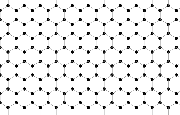
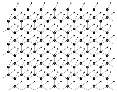
If $\mathbf{W}=(\mathbf{G},m)$ is a weighted graph where $\mathbf{G}$ is either the $\mathbb{Z}^{n}$ -lattice or the graphene lattice (hexagonal lattice consisting of carbon atoms, see Figure 2(a) and 2(b)) both with standard weights, then $\sigma(\Delta^{\mathbf{G}})=[0,2]$ . Hence, the set of spectral gaps is empty, i.e., $\mathcal{S}^{\mathbf{G}}=\emptyset$ and hence $\mathcal{MS}^{\mathbf{G}}=\emptyset$ .

The graphane is just the decoration of the graphene adding an hydrogen atom for each carbon atom (see Figure 2(c)). Here, we have $\sigma(\Delta^{\mathbf{G}})=[0,3/4]\cup[5/4,2]$ for the standard weight, hence $\mathcal{S}^{\mathbf{G}}=(3/4,5/4)$ .

Definition 4.3.

We say that a graph $\mathbf{G}$ has a centre vertex if there exists a vertex $v_{0}$ and a subset $A(v_{0})\subset E_{v_{0}}$ such that $\mathbf{G}-A(v_{0})$ is a tree (and in particular connected). We call the edges in $A(v_{0})$ cycle edges.

A centre vertex is a vertex where all cycles of the graph $\mathbf{G}$ meet. Note that $\{v_{0}\}$ is in the neighbourhood of $A(v_{0})$ (see Definition 3.13).

Is clear that if $\mathbf{G}$ is a tree, then $\mathbf{G}$ does not have a centre vertex (as a tree is connected). Moreover, if $\mathbf{G}$ is a cycle, then any vertex is a centre vertex. By definition, if $\mathbf{G}$ has centre vertex $v_{0}$ , then $b(\mathbf{G})=|A(v_{0})|$ .

We are now able to prove the following sufficient condition for the existence of magnetic gaps (i.e., for $\mathcal{MS}\neq\emptyset$ ). We will use this result (in the case of standard weights) in the examples presented in Section 6. Recall that we allow loops and multiples edges in the graph $\mathbf{G}$ .

Theorem 4.4.

Let $\mathbf{W}=(\mathbf{G},m)$ be a weighted graph. If $v_{0}$ is a centre vertex with cycle edges $A(v_{0})$ and let

\delta:=\rho(v_{0})-\sum_{e\in A(v_{0})}\frac{m_{e}}{m((v_{0})_{e})}-\frac{m(A(v_{0}))}{m(v_{0})}

(4.1)

where $\rho(v_{0})=m(E_{v_{0}}))/m(v)$ is the relative weight at $v_{0}$ . Then the Lebesgue measure of the magnetic spectral gaps set is larger or equal to $\delta$ . In particular, if $\delta>0$ , then $\mathcal{MS}^{\mathbf{W}}\neq\emptyset$ .

Proof.

Let $\alpha$ be any vector potential and consider the virtualised graphs $\mathbf{G}^{-}=\mathbf{G}-A(v_{0})$ and $\mathbf{G}^{+}=\mathbf{G}-\{v_{0}\}$ . As $\mathbf{G}^{-}$ is a tree, we have that $[0,2\rho_{\infty}]\setminus J\subset\mathcal{MS}^{\mathbf{W}}$ , where $J$ is the union of the bracketing interval (cf., Eq. (3.7)). In particular, the measure of $[0,2\rho_{\infty}]\setminus J$ is smaller or equal to the measure of $\mathcal{MS}^{\mathbf{W}}$ . As $\lambda_{1}(\Delta^{\mathbf{W}^{-}})=0$ , the measure of $[0,2\rho_{\infty}]\setminus J$ can be estimated from below by

	$\displaystyle\sum_{k=1}^{n-1}\bigl{(}\lambda_{k+1}\bigl{(}\Delta^{\mathbf{W}^{-}}\bigr{)}-\lambda_{k}\bigl{(}\Delta^{\mathbf{W}^{+}}\bigr{)}\bigr{)}=$	$\displaystyle\sum_{k=1}^{n}\lambda_{k}\bigl{(}\Delta^{\mathbf{W}^{-}}\bigr{)}-\sum_{k=1}^{n-1}\lambda_{k}\bigl{(}\Delta^{\mathbf{W}^{+}}\bigr{)}$
		$\displaystyle=\operatorname{Tr}\bigl{(}\Delta^{\mathbf{W}^{-}}\bigr{)}-\operatorname{Tr}\bigl{(}\Delta^{\mathbf{W}^{+}}\bigr{)},$		(4.2)

so we need to calculate $\operatorname{Tr}\bigl{(}\Delta^{\mathbf{W}^{-}}\bigr{)}$ and $\operatorname{Tr}(\Delta^{\mathbf{W}^{+}})$ (see Proposition 3.3).

Step 1: Trace of $\Delta^{\mathbf{W}^{-}}$ . Let $\mathbf{W}^{-}=(\mathbf{G}^{-},m^{-})$ and recall that $V(\mathbf{G}-A(v_{0}))=V(\mathbf{G})$ , $E(\mathbf{G}-A(v_{0}))=E(\mathbf{G})\setminus A(v_{0})$ ; the weights on $V(\mathbf{G}-A(v_{0}))$ and $E(\mathbf{G}-A(v_{0}))$ coincide with the corresponding weights on $\mathbf{W}$ . The relative weights of $\mathbf{W}^{-}$ are

\rho^{-}(v)=\begin{cases}\rho^{\mathbf{W}}(v)-\dfrac{m\left(E(v)\right)+m\left(A(v_{0})\right)}{m(v)},&\text{if $v=v_{0}$,}\\[8.61108pt] \rho^{\mathbf{W}}(v)-\dfrac{m\left(A(v_{0})\cap E_{v}\right)}{m(v)},&\text{if $v\in B_{v_{0}}$,}\\[8.61108pt] \rho^{\mathbf{W}}(v),&\text{otherwise,}\end{cases}

where

B_{v_{0}}=\{v\in V(\mathbf{G})\mid v=(v_{0})_{e}\text{ for some }e\in A(v_{0})\text{ with }v\neq v_{0}\}.

Since $v_{0}$ is a centre vertex, the only loops (that $\mathbf{G}$ could possibly have) must be attached to $v_{0}$ . The trace of $\Delta^{\mathbf{W}^{-}}$ is now

	$\displaystyle\operatorname{Tr}\bigl{(}\Delta^{\mathbf{W}^{-}}\bigr{)}$	$\displaystyle=\sum_{k=1}^{n}\lambda_{k}\bigl{(}\Delta^{\mathbf{W}^{-}}\bigr{)}=\sum_{v\in V(\mathbf{G})}\rho^{-}(v)$
		$\displaystyle=\sum_{v\in V(\mathbf{G})}\rho^{\mathbf{W}}(v)-\dfrac{m\left(E(v_{0})\right)+m\left(A(v_{0})\right)}{m(v_{0})}-\sum\limits_{v\in B_{v_{0}}}\dfrac{m\left(A(v_{0})\cap E_{v}\right)}{m(v)}.$		(4.3)

Step 2: Trace of $\Delta^{\mathbf{W}^{+}}$ . Let $\mathbf{W}^{+}=\left(\mathbf{G}^{+},m^{+}\right)$ , then the trace of $\Delta^{\mathbf{W}^{+}}$ is given by

\operatorname{Tr}\bigl{(}\Delta^{\mathbf{W}^{+}}\bigr{)}=\sum_{k=1}^{n-1}\lambda_{k}\bigl{(}\Delta^{\mathbf{W}}\bigr{)}=\sum_{\begin{subarray}{c}v\in V(\mathbf{G})\\ v\neq v_{0}\end{subarray}}\rho^{\mathbf{W}}(v).

(4.4)

Combining Equations (4.2), (4.3) and (4.4) we obtain

	$\displaystyle\operatorname{Tr}\bigl{(}\Delta^{\mathbf{W}^{-}}\bigr{)}-\operatorname{Tr}\bigl{(}\Delta^{\mathbf{W}^{+}}\bigr{)}$	$\displaystyle=\rho^{\mathbf{W}}(v_{0})-\frac{m(E(v_{0}))+m(A(v_{0}))}{m(v_{0})}-\sum_{v\in B_{v_{0}}}\frac{m(A(v_{0})\cap E_{v})}{m(v)}$
		$\displaystyle=\rho^{\mathbf{W}}(v_{0})-\frac{m(E(v_{0}))+m\left(A(v_{0})\right)}{m(v_{0})}-\sum_{e\in A(v_{0})\setminus E(v_{0})}\frac{m_{e}}{m((v_{0})_{e})}$
		$\displaystyle=\rho^{\mathbf{W}}(v_{0})-\frac{m\left(A(v_{0})\right)}{m(v_{0})}-\sum_{e\in A(v_{0})}\dfrac{m_{e}}{m((v_{0})_{e})}=\delta$

as defined in Equation (4.1). The last assertion is a simple consequence. ∎

Remark 4.5.

(a)

In the proof, we used the spectral localising inclusion (3.6). If the weighted graph is bipartite and if the weight is normalised (or more generally, if the relative weight is constant), and if we find $B\subset\mathcal{MS}^{\mathbf{W}}$ then we have also $\kappa(B)\subset\mathcal{MS}^{\mathbf{G}}$ by Proposition 2.4.
(b)
For applications, in particular, for the examples of Section 6, we explicitly write Condition 4.1 for the most important weights (see Section 2.2). Let $v_{0}$ be a centre vertex with cycle edges $A(v_{0})$ :
1. (i)
  
  If the graph has the standard weights, the condition becomes:
  
  $\delta=1-\sum_{e\in A(v_{0})}\dfrac{1}{\deg((v_{0})_{e})}-\dfrac{|A(v_{0})|}{\deg(v_{0})}\;,$ (4.5)
  
  where $|A(v_{0})|$ denote the cardinality of the set $A(v_{0})$ .
2. (ii)
  
  Now, if we have the combinatorial weights, the condition becomes simply:
  
  $\delta=\deg(v_{0})-2\;|A(v_{0})|\;.$ (4.6)
3. (iii)
  
  For the electric circuit weights, the condition is:
  
  $\delta=m(E_{v_{0}})-2\;m(A(v_{0}))\;.$ (4.7)
4. (iv)
  
  For the normalised weights, the condition is:
  
  $\delta=1-\sum_{e\in A(v_{0})}\dfrac{m_{e}}{m(E_{(v_{0})_{e}})}-\dfrac{m(A(v_{0}))}{m(E_{v_{0}})}\;.$ (4.8)
In all of the previous cases, if $\mathbf{W}$ is a graph with the corresponding weights and meets the condition $\delta>0$ , then we can assure the existence of magnetic spectral gaps, i.e., $\mathcal{MS}^{\mathbf{W}}\neq\emptyset$ .

Example 4.6.

Consider the next two graphs in Figure 3, both with the standard weights. In both graphs, $v_{0}$ is a centre vertex with cycle edges $A(v_{0})=\left\{e_{1},e_{2}\right\}$ . The strategy to produce gaps is to raise the degree of the vertices $(v_{0})_{e_{1}}$ and $(v_{0})_{e_{2}}$ . In the first case of the Figure 3(a) we have no magnetic spectral gaps, i.e., $\mathcal{MS}^{\mathbf{G}_{1}}=\emptyset$ while for the second graph 3(b) we have

\delta=1-\dfrac{1}{\deg((v_{0})_{e_{1}})}-\dfrac{1}{\deg((v_{0})_{e_{2}})}-\dfrac{2}{\deg(v_{0})}=1-\frac{1}{4}-\frac{1}{5}-\frac{2}{4}=\frac{1}{20}>0,

then $\mathcal{MS}^{\mathbf{G}_{2}}\neq\emptyset$ as a consequence of Theorem 4.4. This example also shows that Condition (4.1) is sufficient but not necessary: consider the graph $\mathbf{G}_{2}$ with only one decorating edge at each vertex $(v_{0})_{e_{1}}$ and $(v_{0})_{e_{2}}$ . The corresponding graph still has a spectral gap, although $\delta=1-1/3-1/3-2/4=-1/6<0$ .

(a) The graph

\mathbf{G}_{1}

(b) The graph

\mathbf{G}_{2}

Figure 3. Producing magnetic spectral gaps by decoration. The graph

\mathbf{G}_{2}

is obtained from

\mathbf{G}_{1}

by adding pendant edges at

(v_{0})_{e_{1}}

and

(v_{0})_{e_{2}}

As a consequence, we have the following topological characterisation for the existence of magnetic spectral gaps for graphs with Betti number $1$ :

Corollary 4.7.

Let $\mathbf{W}=(\mathbf{G},m)$ be a weighted graph with standard weights and Betti number $b(\mathbf{G})=1$ . Then the following conditions are equivalent:

(a)

$\mathbf{G}$ has magnetic spectral gap (i.e., $\mathcal{MS}^{\mathbf{G}}\neq\emptyset$ );
(b)

$\mathbf{G}$ is not a cycle graph;
(c)

$\mathbf{G}$ has a vertex of degree $1$ .

Proof.

“(a) $\Rightarrow$ (b)”: Suppose that $\mathbf{G}=C_{n}$ . Let now $\lambda\in[0,2]$ and $t\in[0,2\pi]$ be such that $\cos t=1-\lambda$ . Consider a vector potential $\alpha$ given by $\alpha_{e}=t$ for all $e\in E(C_{n})$ . We will show that $\lambda\in\sigma(\Delta_{\alpha}^{\mathbf{G}})$ . In fact, consider $\mathbbm{1}(v)=1$ for all $v\in V(\mathbf{G})$ , then

(\Delta_{\alpha}^{\mathbf{W}}\mathbbm{1})(v)=1-\frac{\mathrm{e}^{-it}+\mathrm{e}^{it}}{2}=1-\cos t=\lambda\cdot\mathbbm{1}(v).

We have shown that $[0,2]\subset\bigcup_{\alpha\in\mathcal{A}(\mathbf{G})}\sigma(\Delta^{\mathbf{G}}_{\alpha})$ , i.e., $\mathcal{MS}^{\mathbf{G}}=\emptyset$ .

“(b) $\Rightarrow$ (c)”: Using the fact that $b(\mathbf{G})=1$ , one can prove this by induction on the number of vertices.

“(c) $\Rightarrow$ (a)”: Since $\mathbf{G}$ has Betti number $b(\mathbf{G})=1$ and since $\mathbf{G}$ has a vertex of degree $1$ , there exists $v_{0}\in V(\mathbf{G})$ such that $v_{0}$ belongs to the cycle with $\deg v_{0}\geq 3$ , and it is adjacent with $v_{1}\in V(\mathbf{G})$ by an edge $e_{1}\in E(\mathbf{G})$ with $\deg v_{1}\geq 2$ . Moreover, $v_{0}$ is a centre vertex with cycle edge $A(v_{0})=\left\{e_{1}\right\}$ . As

1-\sum_{e\in A(v_{0})}\dfrac{1}{\deg((v_{0})_{e})}-\dfrac{|A(v_{0})|}{\deg(v_{0})}=1-\frac{1}{\deg_{\mathbf{G}}v_{1}}-\frac{1}{\deg_{\mathbf{G}}v_{0}}\geq 1-\frac{1}{2}-\frac{1}{3}=\dfrac{1}{6}>0,

we conclude from Theorem 4.4 that $\mathcal{MS}^{\mathbf{G}}\neq\emptyset$ .

∎

Remark 4.8.

(a)

Corollary 4.7 holds also for combinatorial weights: for “(a) $\Rightarrow$ (b)” note that $C_{n}$ is a regular graph, hence the spectrum of the standard weight and the combinatorial weight is just related by a simple scaling. For “(c) $\Rightarrow$ (a)” note that the condition on the weights becomes $2=2|A(v_{0})|<3\leq\deg v_{0}$ (choose $v_{0}$ to be the vertex of degree larger than $2$ ). Finally “(b) $\Rightarrow$ (c)” is independent of the weights.
(b)

If the graph $\mathbf{G}$ has the electric circuit weights, then “(a) $\Rightarrow$ (c)” is no longer true. In fact choose $\mathbf{G}=C_{6}$ as in Figure 1 with $m_{e}=1$ if $e\neq e_{1}$ and $m_{e_{1}}=2$ . For example, an easy calculation show that $0$ and $1\in\sigma(\Delta^{\mathbf{W}})$ but $0.3\in\mathcal{MS}^{\mathbf{W}}$ , then $\mathcal{MS}^{\mathbf{W}}\neq\emptyset$ even if there is no any vertex of degree $1$ .
(c)

If the graph $\mathbf{G}$ has normalised weights, then in general “(a) $\Rightarrow$ (c)” is not true. Choose $\mathbf{G}=C_{6}$ as in Figure 1 with the following weights: on the edges $m_{e}=1$ if $e\neq e_{1}$ and $m_{e_{1}}=2$ , on the vertices $m(v_{i})=2$ for $i=1,2$ and $m(v_{i})=1$ for $i=3,4,5,6$ . It is easy to check that $0$ and $1\in\sigma(\Delta^{\mathbf{W}})$ with $1/2\in\mathcal{MS}^{\mathbf{W}}$ . Then $\mathcal{MS}^{\mathbf{W}}\neq\emptyset$ but again, there is no vertex of degree $1$ .

Example 4.9.

Let $\mathbf{W}^{\prime}=(\mathbf{G}^{\prime},m^{\prime})$ where $\mathbf{G}^{\prime}=C_{6}$ and $m^{\prime}$ are the standard weights, then by Corollary 4.7 we have $\mathcal{MS}^{\mathbf{G}^{\prime}}=\emptyset$ . In order to create magnetic spectral gaps we add a new edge. Let now $\mathbf{W}=(\mathbf{G},m)$ where $\mathbf{G}$ is the graph $C_{6}$ with an edge added to the cycle (see Figure 4) and $m$ the standard weights. Then the Laplacian on $\mathbf{G}$ has a magnetic spectral gap by Corollary 4.7. Now using the bracketing technique of Theorem 3.14 we can localise the position of the gaps.

Consider $E_{0}=\{e_{1}\}$ , and recall that any vector potential $\alpha$ can be supported on $e_{1}$ . Consider also the edge virtualised weighted graph $\mathbf{W}^{-}=(\mathbf{G}^{-},m^{-})$ with $\mathbf{G}^{-}=\mathbf{G}-E_{0}$ . Then its spectrum is:

\sigma\bigl{(}\Delta^{\mathbf{W}^{-}}\bigr{)}\approx\{0,0.116,0.5,0.713,1.145,1.638,1.889\}.

Now, we have that $V_{0}=\{v_{1}\}$ is in the neighbourhood of $E_{0}$ . Now consider the vertex virtualised weighted graph $\mathbf{W}^{+}=(\mathbf{G}^{+},m^{+})$ with $\mathbf{G}^{+}=\mathbf{G}-V_{0}$ , then its spectrum is:

\sigma\bigl{(}\Delta^{\mathbf{W}^{+}}\bigr{)}\approx\{0.121,0.358,0.744,1.256,1.642,1.879,2\}.

Therefore, the bracketing intervals in which we can localise the spectrum is given by (see Figure 4):

	$\displaystyle J_{1}\approx\left[0,0.121\right],\quad J_{2}\approx\left[0.116,0.358\right],\quad J_{3}\approx\left[0.5,0.744\right],\quad J_{4}\approx\left[0.713,1.256\right],$
	$\displaystyle J_{5}\approx\left[1.145,1.642\right],\quad J_{6}\approx\left[1.638,1.879\right],\quad and\quad J_{7}\approx\left[1.889,2\right].$

In conclusion, we have the following spectral localising inclusion for any vector potential $\alpha$ :

\bigcup_{\alpha\in\mathcal{A}(\mathbf{G})}\sigma(\Delta^{\mathbf{G}}_{\alpha})\subset J=\bigcup_{k=1}^{7}J_{i}\subsetneq[0,2].

(4.9)

Figure 4. Example of bracketing intervals for the cycle graph

C_{6}

with one pendant edge.

5. Periodic graphs

We begin recalling the definition and some useful facts concerning periodic graphs, discrete Floquet theory and its relation to the vector potential.

5.1. Periodic graphs and fundamental domains

The preceding two sections refer to finite graphs. We consider here certain classes of infinite graphs, namely $\Gamma$ -periodic graphs, where $\Gamma=\left\langle g_{1},g_{2},\dots,g_{r}\right\rangle$ is a finitely generated and Abelian group with generators $g_{1},g_{2},\dots,g_{r}$ . In crystallography, one typically considers $\Gamma=\mathbb{Z}^{r}$ (see [Sun13, Sec. 6.2]), with generators given, for example, by $g_{1}=\left(1,0,\dots,0\right),g_{2}=\left(0,1,\dots,0\right),\dots,g_{r}=\left(0,0,\dots,1\right)$ . We say that a graph $\widetilde{\mathbf{G}}$ is $\Gamma$ -periodic if there is a free and transitive action of $\Gamma$ on $\widetilde{\mathbf{G}}$ with compact quotient $\mathbf{G}=\widetilde{\mathbf{G}}/\Gamma$ and which is orientation preserving, i.e., $\Gamma$ acts both on $V$ and $E$ such that

\partial_{+}(\gamma e)=\gamma(\partial_{+}e)\quad\text{and}\quad\partial_{-}(\gamma e)=\gamma(\partial_{-}e)\qquad\text{for all $\gamma\in\Gamma$ and $e\in E$.}

To avoid trivial situations we assume that the periodic graph $\widetilde{\mathbf{G}}$ is connected. As we use the multiplicative notation for the action, we also write $\Gamma$ multiplicatively. In particular, we have

E_{\gamma v}=\gamma E_{v}\qquad\text{for all $\gamma\in\Gamma$ and $e\in E$.}

A $\Gamma$ -periodic graph $\widetilde{\mathbf{G}}$ can also be seen as a covering (see [Sun13, Ch. 5 and 6] or [Sun08] for more details):

\pi\colon\widetilde{\mathbf{G}}\rightarrow\mathbf{G}=\widetilde{\mathbf{G}}/\Gamma.

We say that a weighted graph $\widetilde{\mathbf{W}}=(\widetilde{\mathbf{G}},\widetilde{m})$ is $\Gamma$ -periodic if $\widetilde{\mathbf{G}}$ is $\Gamma$ -periodic and if the action of $\Gamma$ on $\widetilde{\mathbf{G}}$ preserves the corresponding weights, i.e., if

\widetilde{m}(\gamma v)=\widetilde{m}(v)\quad\text{for all $v\in V$}\qquad\text{and}\qquad\widetilde{m}_{\gamma e}=\widetilde{m}_{e}\quad\text{for all $e\in E$ and $\gamma\in\Gamma$.}

Note that the standard or combinatorial weights on a discrete graph satisfy these conditions automatically. A $\Gamma$ -periodic weighted graph $\widetilde{\mathbf{W}}=(\widetilde{\mathbf{G}},\widetilde{m})$ naturally induces a weight $m$ on the quotient graph, given by $\widetilde{m}\circ\pi^{-1}$ . Notice that this weight is well-defined since $\widetilde{m}$ is $\Gamma$ -invariant. We will denote this weight on the quotient simply by $m$ .

We consider first the following convenient notation adapted to the description of periodic graphs (see, e.g., [LP08b, Sec. 7]) and the important notion of an edge index (see [KS14, Subsections 1.2 and 1.3]

Definition 5.1.

Let $\widetilde{\mathbf{G}}=(V,E,\partial)$ be a $\Gamma$ -periodic graph.

(a)

A vertex, respectively edge fundamental domain on a $\Gamma$ -periodic graph is given by two subsets $D^{V}\subset V$ and $D^{E}\subset E$ satisfying

	$\displaystyle V(\widetilde{\mathbf{G}})$	$\displaystyle=\bigcup_{\gamma\in\Gamma}\gamma D^{V}\quad\text{and}\quad\gamma_{1}D^{V}\cap\gamma_{2}D^{V}=\emptyset\quad\text{if $\gamma_{1}\neq\gamma_{2}$,}$
	$\displaystyle E(\widetilde{\mathbf{G}})$	$\displaystyle=\bigcup_{\gamma\in\Gamma}\gamma D^{E}\quad\text{and}\quad\gamma_{1}D^{E}\cap\gamma_{2}D^{E}=\emptyset\quad\text{if $\gamma_{1}\neq\gamma_{2}$}$

with $D^{E}\cap E(V\setminus D^{V})=\emptyset$ (i.e., an edge in $D^{E}$ has at least one endpoint in $D^{V}$ ). We often simply write $D$ for a fundamental domain, where $D$ stands either for $D^{V}$ or $D^{E}$ .

(b)

A (graph) fundamental domain of a periodic graph $\widetilde{\mathbf{G}}$ is a partial subgraph

$\mathbf{H}=(D^{V},D^{E},\partial\restriction_{D^{E}}),$

where $D^{V}$ and $D^{E}$ are vertex and edge fundamental domains, respectively. We call

$B(\mathbf{H},\widetilde{\mathbf{G}}):=E(D^{V},V\setminus D^{V})$

the set of connecting edges of the fundamental domain $\mathbf{H}$ in $\widetilde{\mathbf{G}}$ .²²2 In [KS14], Korotyaev and Saburova used the term bridge for all edges connecting a fundamental domain with another (non-trivial) translate of the fundamental domain. Korotyaev and Saburova have hence twice as many such edges as we have in $B(\mathbf{H},\mathbf{G})$ . Although the name “bridge” is quite intuitive, it is already used in graph theory in a different context; namely for an edge that disconnects a graph if it is removed.

Remark 5.2.

(a)

Note that once a fundamental domain $D^{V}$ has been specified in a $\Gamma$ -periodic graph $\widetilde{\mathbf{G}}$ , we can write any $v\in V(\widetilde{\mathbf{G}})$ uniquely as $v=\xi(v)v_{0}$ for a unique pair $(\xi(v),v_{0})\in\Gamma\times D^{V}$ . This follows from the fact that the action is free and transitive. We call $\xi(v)$ the $\Gamma$ -coordinate of $v$ (with respect to the fundamental domain $D^{V}$ ). Similarly we can define the coordinates for the edges: any $e\in E(\widetilde{\mathbf{G}})$ can be written as $e=\xi(e)e_{0}$ for a unique pair $(\xi(e),e_{0})\in\Gamma\times D^{E}$ . In particular, we have

$\xi(\gamma v)=\gamma\xi(v)\qquad\text{and}\qquad\xi(\gamma e)=\gamma\xi(e).$

(b)

Once we have chosen a fundamental domain $\mathbf{H}=(D^{V},D^{E},\partial)$ , we can embed $\mathbf{H}$ it into the quotient $\mathbf{G}=\widetilde{\mathbf{G}}/\Gamma$ of the covering $\pi\colon\widetilde{\mathbf{G}}\rightarrow\mathbf{G}=\widetilde{\mathbf{G}}/\Gamma$ by

D^{V}\rightarrow V(\mathbf{G})=V/\Gamma,\quad v\mapsto[v]\qquad\text{and}\qquad D^{E}\rightarrow E(\mathbf{G})=E/\Gamma,\quad e\mapsto[e],

where $[v]$ and $[e]$ denote the $\Gamma$ -orbits of $v$ and $e$ , respectively. By definition of a fundamental domain, these maps are bijective. Moreover, if $\partial_{\pm}e=v$ in $\mathbf{H}$ , then also $\partial_{\pm}([e])=[v]$ in $\mathbf{G}$ , i.e., the embedding is a (partial) graph homomorphism.

Definition 5.3.

Let $\widetilde{\mathbf{G}}=(V,E,\partial)$ be a $\Gamma$ -periodic graph with fundamental graph $\mathbf{H}=(D^{V},D^{E},\partial)$ . We define the index of an edge $e\in E$ as

\operatorname{ind}_{\mathbf{H}}(e):=\xi(\partial_{+}e)\left(\xi(\partial_{-}e)\right)^{-1}\in\Gamma.

In particular, we have $\operatorname{ind}_{\mathbf{H}}\colon E\mapsto\Gamma$ , and $\operatorname{ind}_{\mathbf{H}}(e)\neq 1_{\Gamma}$ iff $e\in\bigcup_{\gamma\in\Gamma}\gamma B(\mathbf{H},\widetilde{\mathbf{G}})$ , i.e., the index is only non-trivial on the (translates of the) connecting edges. Moreover, the set of indices and its inverses generate the group $\Gamma$ .

Since the index fulfils $\operatorname{ind}_{\mathbf{H}}(\gamma e)=\gamma\operatorname{ind}_{\mathbf{H}}(e)$ for all $\gamma\in\Gamma$ by Remark 5.2 (a), we can extend the definition to the quotient $\mathbf{G}=\widetilde{\mathbf{G}}/\Gamma$ by setting $\operatorname{ind}_{\mathbf{G}}([e])=\operatorname{ind}_{\mathbf{H}}(e)$ for all $e\in E(\widetilde{\mathbf{G}})$ . We denote also $[B(\mathbf{H},\widetilde{\mathbf{G}})]:=\{[e]\mid e\in B(\mathbf{H},\widetilde{\mathbf{G}})\}$ .

5.2. Discrete Floquet theory

Let $\widetilde{\mathbf{W}}=(V,E,\partial,\widetilde{m})$ be a weighted $\Gamma$ -periodic graph and fundamental domain $\mathbf{H}=(D^{V},D^{E},\partial)$ with corresponding weights inherited from $\widetilde{\mathbf{W}}$ . In this context one has the natural Hilbert space identifications

\ell_{2}(V,\widetilde{m})\cong\ell_{2}(\Gamma)\otimes\ell_{2}(D^{V},m)\cong\ell_{2}\bigl{(}\Gamma,\ell_{2}(D^{V},m)\bigr{)}.

Roughly speaking, a discrete Floquet transformation is a partial Fourier transformation which is applied only on the group part, i.e.,

F\colon\ell_{2}(\Gamma)\rightarrow L_{2}(\widehat{\Gamma}),\qquad\left(F\mathbf{a}\right)\left(\chi\right):=\sum_{\gamma\in\Gamma}\overline{\chi(\gamma)}a_{\gamma}

for $\mathbf{a}=\left\{a_{\gamma}\right\}_{\gamma\in\Gamma}\in\ell_{2}(\Gamma)$ and where $\widehat{\Gamma}$ denotes the character group of $\Gamma$ . We adapt to the discrete context of graphs the main results concerning Floquet theory needed later. We refer to [LP07, Section 3] as well as [KS14] for details and additional motivation.

For any character $\chi\in\widehat{\Gamma}$ consider the space of equivariant functions on vertices and edges

	$\displaystyle\ell_{2}^{\chi}(V,m)$	$\displaystyle:=$	$\displaystyle\left\{g\colon V\rightarrow\mathbb{C}\mid g(\gamma v)=\chi(\gamma)g(v)\text{ for all }v\in V\text{ and }\gamma\in\Gamma\right\},$
	$\displaystyle\ell_{2}^{\chi}(E,m)$	$\displaystyle:=$	$\displaystyle\left\{\eta\colon E\rightarrow\mathbb{C}\mid\eta_{\gamma e}=\chi(\gamma)\eta_{e}\text{ for all }e\in E\text{ and }\gamma\in\Gamma\right\}.$

These spaces have the natural inner product:

\left\langle g_{1},g_{2}\right\rangle:=\sum_{v\in D^{V}}g_{1}(v)\overline{g_{2}(v)}m(v)

for a fundamental domain $D^{V}$ (and similarly for the equivariant scalar product on $D^{E}$ ). Note that the definition of the inner product is independent of the choice of fundamental domain (due to the equivariance). The following decomposition result is standard, see, for example, [KS14] or [HS99].

Proposition 5.4.

Let $\widetilde{\mathbf{W}}=(\widetilde{\mathbf{G}},\widetilde{m})$ be a periodic weighted graph with $\widetilde{\mathbf{G}}=(V,E,\partial)$ . Then there is a unitary transformation

\Phi\colon\ell_{2}(V(\widetilde{\mathbf{G}}))\rightarrow\int_{\widehat{\Gamma}}^{\oplus}\ell_{2}^{\chi}(V,m)\,\mathrm{d}\chi\qquad\text{given by}\qquad\left(\Phi f\right)_{\chi}(v)=\sum_{\gamma\in\Gamma}\overline{\chi({\gamma})}f(\gamma v)

such that

\sigma\bigl{(}\Delta^{\!\widetilde{\mathbf{W}}}\bigr{)}=\bigcup_{\chi\in\widehat{\Gamma}}\sigma\bigl{(}\prescript{\chi\!}{}{\Delta}^{\!\widetilde{\mathbf{W}}}{}\bigr{)}.

where as $\prescript{\chi\!}{}{\Delta}^{\!\widetilde{\mathbf{W}}}{}:=\Delta^{\!\widetilde{\mathbf{W}}}\restriction_{\ell_{2}^{\chi}(V,m)}$ denotes the equivariant Laplacian.

The equivariant Laplacian may also be described in terms of a first order approach by defining $d^{\chi}\colon\ell_{2}^{\chi}(V,m)\to\ell_{2}^{\chi}(E,m)$ just by restriction of $d$ to the subspace $\ell_{2}^{\chi}(V,m)$ :

(d^{\chi}g)_{e}=g(\partial_{+}e)-g(\partial_{-}e)\;,\quad g\in\ell_{2}^{\chi}(V,m)\;.

It is straightforward to check that $d^{\chi}g\in\ell_{2}^{\chi}(E,m)$ if $g\in\ell_{2}^{\chi}(V,m)$ and that $\prescript{\chi\!}{}{\Delta}^{\!\widetilde{\mathbf{W}}}{}=(d^{\chi})^{*}d^{\chi}$ .

5.3. Vector potential as a Floquet parameter

The following result shows that in the case of Abelian groups $\Gamma$ the vector potential can be interpreted as a Floquet parameter of the periodic graph $\widetilde{\mathbf{G}}\to\mathbf{G}$ (see Remark 5.2 (b)). Consider the following unitary maps (see also [KOS89] for manifolds):

	$\displaystyle U^{V}$	$\displaystyle\colon\ell_{2}(V(\mathbf{G}),m)\to\ell_{2}^{\chi}(V,m),$	$\displaystyle\bigl{(}U^{V}f\bigr{)}(v)$	$\displaystyle=\chi(\xi(v))f([v]),$
	$\displaystyle U^{E}$	$\displaystyle\colon\ell_{2}(E(\mathbf{G}),m)\to\ell_{2}^{\chi}(E,m),$	$\displaystyle\bigl{(}U^{E}\eta\bigr{)}_{e}$	$\displaystyle=\chi(\xi(e))\left(\eta\right)_{[e]}.$

It is straightforward to see that $U^{V}f\in\ell_{2}^{\chi}(V,m)$ for all $f\in\ell_{2}(V(\mathbf{G}),m)$ and that $U^{V}$ is unitary (similarly for $U^{E}$ ).

Definition 5.5.

Let $\widetilde{\mathbf{W}}=(\widetilde{\mathbf{G}},\widetilde{m})$ be a $\Gamma$ -periodic weighted graph with finite quotient $\mathbf{W}=(\mathbf{G},m)$ and $\mathbf{H}$ be a fundamental domain. If $\alpha$ is a vector potential acting on $\mathbf{G}$ , we say that $\alpha$ has the lifting property if there exists $\chi\in\widehat{\Gamma}$ such that:

\mathrm{e}^{i\alpha_{[e]}}=\chi\left(\operatorname{ind}_{\mathbf{H}}(e)\right)\quad\text{ for all }e\in E(\widetilde{\mathbf{G}}).

(5.1)

We denote the set of all the vector potentials with the lifting property as $\mathcal{A}_{\mathbf{H}}$ .

Proposition 5.6.

\sigma(\Delta^{\!\widetilde{\mathbf{W}}})=\bigcup_{\alpha\in\mathcal{A}_{\mathbf{H}}}\sigma(\Delta^{\mathbf{W}}_{\alpha})\subset[0,2p_{\infty}]\setminus\mathcal{MS}^{\mathbf{W}}.

(5.2)

Proof.

By Proposition 5.4, it is enough to show

\bigcup_{\chi\in\widehat{\Gamma}}\sigma\bigl{(}\prescript{\chi\!}{}{\Delta}^{\!\widetilde{\mathbf{W}}}{}\bigr{)}=\bigcup_{\alpha\in\mathcal{A}_{\mathbf{H}}}\sigma\bigl{(}\Delta^{\mathbf{W}}_{\alpha}\bigr{)}

“ $\subset$ ”: Consider a character $\chi\in\widehat{\Gamma}$ and define a vector potential on $\mathbf{G}$ as follows

\mathrm{e}^{\mathrm{i}\alpha_{[e]}}=\chi(\operatorname{ind}_{\mathbf{H}}(e))\;,\quad e\in E\;.

(5.3)

Then we have

(d^{\chi}U^{V}f)_{e}=(U^{V}f)(\partial_{+}e)-(U^{V}f)(\partial_{-}e)=\chi(\xi(\partial_{+}e))f([\partial_{+}e])-\chi(\xi(\partial_{-}e))f([\partial_{-}e]).

On the other hand, we have

(U^{E}d_{\alpha}f)_{e}=\chi(\xi(e))\Bigl{(}\mathrm{e}^{\mathrm{i}\alpha_{[e]}/2}f([\partial_{+}e])-\mathrm{e}^{-\mathrm{i}\alpha_{[e]}/2}f([\partial_{-}e])\Bigr{)}.

Therefore, the intertwining equation $d^{\chi}U^{V}=U^{E}d_{\alpha}$ holds if

\chi(\xi(\partial_{+}e))=\chi(\xi(e))\mathrm{e}^{\mathrm{i}\alpha_{[e]}/2}\quad\text{and}\quad\chi(\xi(\partial_{-}e))=\chi(\xi(e))\mathrm{e}^{-\mathrm{i}\alpha_{[e]}/2}

or, equivalently, if

\chi(\xi(\partial_{+}e))\mathrm{e}^{-\mathrm{i}\alpha_{[e]}/2}=\chi(\xi(\partial_{-}e))\mathrm{e}^{\mathrm{i}\alpha_{[e]}/2}

\mathrm{e}^{\mathrm{i}\alpha_{[e]}}=\chi(\xi(\partial_{+}e))\chi(\xi(\partial_{-}e))^{-1}=\chi(\operatorname{ind}_{\mathbf{H}}(e))\;.

But this equation is true by definition of the vector potential on $\mathbf{G}$ given in Equation (5.3). Finally, since $\prescript{\chi\!}{}{\Delta}^{\!\widetilde{\mathbf{W}}}{}=(d^{\chi})^{*}d^{\chi}$ and $\Delta^{\mathbf{W}}_{\alpha}=d_{\alpha}^{*}d_{\alpha}$ it is clear that these Laplacians are unitarily equivalent.

“ $\supset$ ”: Let $\alpha\in\mathcal{A}_{\mathbf{H}}$ and $E_{\mathbf{H}}\subset E(\mathbf{G})$ is such that $\{\operatorname{ind}_{\mathbf{H}}(e)|[e]\in E_{\mathbf{H}}\}$ is a basis of the group $\Gamma$ . Then define

\chi(\operatorname{ind}_{\mathbf{H}}(e))=\mathrm{e}^{\mathrm{i}\alpha_{[e]}}\;,\quad e\in E_{\mathbf{H}}\;.

(5.4)

so we can extend $\chi$ to all $\Gamma$ , so $\chi\in\widehat{\Gamma}$ . As before, we can show $\sigma\bigl{(}\prescript{\chi\!}{}{\Delta}^{\!\widetilde{\mathbf{W}}}{}\bigr{)}=\sigma\left(\Delta^{\mathbf{W}}_{\alpha}\right).$ ∎

Remark 5.7.

(a)

If $\widetilde{\mathbf{G}}\to\mathbf{G}$ is a maximal Abelian covering, then we have $\sigma(\Delta^{\widetilde{\mathbf{G}}})=[0,2p_{\infty}]\setminus\mathcal{MS}^{\mathbf{G}}$ . In particular, this is true if $\widetilde{\mathbf{G}}$ is a tree.

(b)

If $\Gamma=\mathbb{Z}$ and if each fundamental domain is connected to its neighbours by a single connecting edge, i.e., $|B(\mathbf{H},\widetilde{\mathbf{G}})|=1$ then we have the following situation: Define the vector potential $\alpha^{t}$ on $\mathbf{G}$ as $\alpha^{t}=t$ if $[e]\in[B(\mathbf{H},\widetilde{\mathbf{G}})]$ and zero otherwise. Denote $\sigma\left(\Delta^{\widetilde{\mathbf{G}}}_{\alpha^{t}}\right):=\{\lambda^{t}_{i}\mid i=1,\dots,n\}$ be the eigenvalues in ascending order and repeated according to their multiplicities, then following results in [EKW10] we obtain

\sigma(\Delta^{\widetilde{\mathbf{G}}})=\bigcup_{i=1}^{|V(\mathbf{G})|}\bigl{[}\min\bigl{\{}\lambda^{0}_{i},\lambda^{\pi}_{i}\bigr{\}},\max\bigl{\{}\lambda^{0}_{i},\lambda^{\pi}_{i}\bigr{\}}\bigr{]}.

Let $\mathbf{W}=(\mathbf{G},m)$ a weighted graph. We say that $\mathbf{W}$ has the Full spectrum property (FSP) if $\Delta^{\mathbf{W}}=[0,2\rho_{\infty}]$ . In fact, $\mathbf{W}$ has the FSP iff $\mathcal{S}^{\mathbf{W}}=\emptyset$ . The next conjecture is stated in [HS99]. Let $\widetilde{\mathbf{G}}$ be a maximal Abelian covering of $\mathbf{G}$ , if $\mathbf{G}$ has no vertex of degree $1$ then $\widetilde{\mathbf{G}}$ has the FSP. Moreover, Higuchi and Shirai propose the next problem: Characterise all finite graphs whose maximal Abelian covering do not has the FSP. Here, we partially solve the conjecture and the problem.

The following result verifies Higuchi-Shirai’s conjecture in [HS04] for $\mathbb{Z}$ -periodic trees.

Theorem 5.8.

(a)

$\widetilde{\mathbf{W}}$ has the full spectrum property;
(b)

$\mathcal{S}^{\widetilde{\mathbf{W}}}=\emptyset$ ;
(c)

$\widetilde{\mathbf{G}}$ is the lattice $\mathbb{Z}$ ;
(d)

$\mathcal{MS}^{\mathbf{W}}=\emptyset$ ;
(e)

$\mathbf{G}$ is a cycle graph;
(f)

$\mathbf{G}$ has no vertex of degree $1$ .

Proof.

In this situation $\widetilde{\mathbf{G}}\to\mathbf{G}$ is a maximal Abelian covering if and only if the Betti number $b(\mathbf{G})=1$ if and only if $\widetilde{\mathbf{G}}$ is a $\mathbb{Z}$ -periodic tree. Since $\widetilde{\mathbf{G}}$ is a tree and $\widetilde{\mathbf{G}}\to\mathbf{G}$ is a maximal Abelian covering, then we have $\sigma(\Delta^{\!\widetilde{\mathbf{W}}})=[0,2p_{\infty}]\setminus\mathcal{MS}^{\mathbf{W}}$ . The result then follows by Corollary 4.7. ∎

Remark 5.9.

Example 6.2 confirms the previous theorem. In addition, if $b(\mathbf{G})\geq 2$ one can easily produce periodic graphs based, e.g., on Example 4.6 that do not having the full spectrum property.

5.4. Discrete bracketing technique

We apply now the technique stated in Proposition 3.3 to periodic graphs.

Theorem 5.10.

Let $\widetilde{\mathbf{W}}=(\widetilde{\mathbf{G}},\widetilde{m})$ a $\Gamma$ -periodic graph and $\pi\colon\widetilde{\mathbf{G}}\rightarrow\mathbf{G}=\widetilde{\mathbf{G}}/\Gamma$ with fundamental domain $\mathbf{H}=(D^{V},D^{E},\partial)$ . We let

E_{0}:=[B(\mathbf{H},\widetilde{\mathbf{G}})]

be the image of the connectivity edges on the quotient and $V_{0}$ in the neighbourhood of $E_{0}$ . Define by

\mathbf{G}^{-}:=\mathbf{G}-E_{0}\qquad\text{and}\qquad\mathbf{G}^{+}:=\mathbf{G}-V_{0}.

the corresponding edge and vertex virtualised partial graphs, respectively. Then

\sigma(\Delta^{\!\widetilde{\mathbf{W}}})\subset\bigcup_{k=1}^{|V(\mathbf{G})|}\underbrace{[\lambda_{k}(\Delta^{\mathbf{G}^{-}}),\lambda_{k}(\Delta^{\mathbf{G}^{+}})]}_{=:J_{k}}

where $\sigma(\Delta^{\mathbf{G}^{-}})$ and $\sigma(\Delta^{\mathbf{G}^{+}})$ are as in Theorem 3.14, i.e., the eigenvalues are written in ascending order and repeated according to their multiplicities.

Proof.

By Proposition 5.6 we have

\sigma(\Delta^{\!\widetilde{\mathbf{W}}})=\bigcup_{\alpha\in\mathcal{A}_{\mathbf{H}}}\sigma(\Delta^{\mathbf{W}}_{\alpha}).

Now, by the bracketing technique of Propositions 3.6 and 3.11, we have for any potential $\alpha\in\mathcal{A}_{\mathbf{H}}$ ,

\lambda_{k}(\Delta^{\mathbf{G}^{-}})\leq\lambda_{k}(\Delta^{\mathbf{G}}_{\alpha})\leq\lambda_{k}(\Delta^{\mathbf{G}^{+}})\quad\text{for all}\quad k=1,\dots,|V(\mathbf{G})|

provided the vector potential is supported only on the (translates of the) connecting edges $E_{0}\subset E(\mathbf{G})$ . Therefore

\sigma(\Delta^{\!\widetilde{\mathbf{W}}})\subset\bigcup_{k=1}^{|V(\mathbf{G})|}\underbrace{[\lambda_{k}(\Delta^{\mathbf{G}^{-}}),\lambda_{k}(\Delta^{\mathbf{G}^{+}})]}_{=:J_{k}}.\qed

Note that the bracketing intervals $J_{k}$ depend on the fundamental domain $\mathbf{H}$ . A good choice would be one where the set of connecting edges is as small as possible. In this case, we have a good chance that the bracketing intervals $J_{k}$ actually do not cover the full interval $[0,2\rho_{\infty}]$ . This is geometrically a “thin–thick” decomposition, just as in [LP08a], where a fundamental domain only has a few connections to the complement.

6. Examples and applications: Spectral gaps for periodic graphs

We conclude this article with several applications of the methods developed before. Our first example confirms the results by Suzuki in [Suz13] on periodic graphs with pendants edges using our simple geometric method (Example 6.1). The other examples are more elaborate and include an idealised model of polypropylene (Example 6.2) and polyacetylene molecules (Example 6.3). The last example can be understood as an intermediate covering of graphane and shows that the bracketing technique developed here extends to more general situation than the $\mathbb{Z}$ -periodic trees, i.e., to higher Betti numbers of the quotient graphs.

Example 6.1 (Suzuki’s example).

Consider the graph $T_{n}$ consisting of the $\mathbb{Z}$ -lattice and a pendant edge at every $n$ -th vertex as decoration (see Figure 5) with standard weights as in [Suz13]. It is easy to see that the tree $T_{n}$ is the maximal Abelian covering graph of $\mathbf{G}_{n}$ , where $\mathbf{G}_{n}$ is just the cycle graph $C_{n}$ decorated with an additional edge attached to some vertex of the cycle (for example see Figure 4 for $\mathbf{G}_{6}$ ) with the standard weights. The graph $T_{n}$ has spectral gaps, i.e., $\mathcal{S}^{T_{n}}\neq\emptyset$ , as Suzuki proves. Our analysis allows an alternative and short proof (based on the criterion in Corollary 4.7): As $T_{n}$ is a tree, we can apply Theorem 5.8: as $\mathbf{G}_{n}$ has a vertex of degree $1$ , the covering graph $T_{n}$ cannot have the full spectrum property.

Figure 5. The infinite tree graph

T_{n}

with a pendant vertex every

n

vertices along the

\mathbb{Z}

-lattice, see [Suz13].

Example 6.2 (Polypropylene).

Consider the graph associated to a thermoplastic polymer, the polypropylene. This structure consists of a sequence of carbon atoms (white vertices) with hydrogen (black vertices) and the methyl group $\mathrm{CH}_{3}$ . We choose the infinite covering graph $\widetilde{\mathbf{G}}$ as an idealised model of polypropylene (see Figure 6(a)); this graph is a covering graph of the bipartite graph denoted as $\mathbf{G}$ (see Figure 6(b)). Again, by Corollary 4.7 we get that the set of magnetic spectral gaps is not empty $\mathcal{MS}^{\mathbf{G}}\neq 0$ and by Proposition 5.6 we conclude that the Laplacian on $\widetilde{\mathbf{G}}$ has spectral gaps. We show how to apply the technique developed in this article twice:

First, let $E_{0}=\{e_{1}\}$ . Then $V_{0}=\{v_{1}\}$ is in the neighbourhood of $E_{0}$ (see Definition 3.13). Using the notation in Theorem 3.14 and Proposition 5.6 we get $\sigma(\Delta^{\widetilde{\mathbf{G}}})\subset J$ , where $J$ is a subset of $[0,2]$ (see Figure 6(c)). Since $\mathbf{G}$ is bipartite we obtain $\sigma(\Delta^{\widetilde{\mathbf{G}}})\subset\kappa(J)$ by Proposition 2.4. Therefore, the symmetry gives tighter localisation of the spectrum $\sigma(\Delta^{\widetilde{\mathbf{G}}})\subset J\cap\kappa(J)$ .

But the set $V_{0}^{\prime}=\{v_{2}\}$ is also in the neighbourhood of the previous set $E_{0}$ . Then apply the same argument as before for $E_{0}$ and $V_{0}^{\prime}$ to obtain $J^{\prime},\kappa(J^{\prime})$ . Again we obtain $\sigma(\Delta^{\widetilde{\mathbf{G}}})\subset J^{\prime}\cap\kappa(J^{\prime})$ . We conclude that $\sigma(\Delta^{\widetilde{\mathbf{G}}})\subset J\cap\kappa(J)\cap J^{\prime}\cap\kappa(J^{\prime})$ . In fact, in Figure 6(c) we see that our technique gives a very good estimation for the spectrum.

(a) The covering graph

\widetilde{\mathbf{G}}

modelling prolypropylene.

(b) The quotient graph

\mathbf{G}

\widetilde{\mathbf{G}}

and the spectral localisation.

Figure 6. Spectral gaps of polypropylene.

J

is the spectral localisation of the pair

\mathbf{G}-\{e_{1}\}

and

\mathbf{G}-\{v_{1}\}

, and bipartiteness gives

J\cap\kappa(J)

as localisation set. Similarly,

J^{\prime}

is the spectral localisation of the pair

\mathbf{G}-\{e_{1}\}

and

\mathbf{G}-\{v_{2}\}

. Putting all this information together, we get the rather good spectral localisation

J\cap\kappa(J)\cap J^{\prime}\cap\kappa(J^{\prime})

Example 6.3 (Polyacetylene).

The previous examples show the existence of spectral gaps in periodic trees covering finite graphs with Betti number $1$ . In this example we show how to treat more complex periodic graphs. Consider the polyacetylene, that consists of a chain of carbon atoms (white circles) with alternating single and double bonds between them, each with one hydrogen atoms (black vertex). We denote this graph as $\widetilde{\mathbf{G}}$ and note that it is not a tree (cf., Figure 7(a)). If we want to compute $\sigma(\Delta^{\widetilde{\mathbf{G}}})$ we use Proposition 5.6. The graph $\widetilde{\mathbf{G}}$ is covering the graph $\mathbf{G}$ (see Figure 7(b)) which is bipartite and has Betti number $2$ . In this case,

\sigma(\Delta^{\widetilde{\mathbf{G}}})=\bigcup_{t\in[0,2\pi]}\sigma(\Delta^{\mathbf{G}}_{\alpha^{t}})

where ${\alpha^{t}}$ is supported only in $e_{1}$ with $\alpha^{t}_{e_{1}}=t$ (see Remark 5.7).

As in the previous examples, we assume that the vector potential $\alpha$ is supported only on one edge, say $e_{1}$ . Define $E_{0}=\{e_{1}\}$ and $V_{0}=\{v_{1}\}$ , then $V_{0}$ is in the neighbourhood of $E_{0}$ . We proceed as in the previous example to localise the spectrum within $J\cap\kappa(J)$ (see Figure 7). In fact, our method works almost perfectly in this case, since we detect precisely the spectrum

J\cap\kappa(J)\setminus{\{1\}}=\sigma(\Delta^{\widetilde{\mathbf{G}}}).

(a) Polyacetylene modelled by the covering graph

\widetilde{\mathbf{G}}

(b) The quotient graph

\mathbf{G}

(c)

Figure 7. Spectral gaps of polyacetylene. This is an example where the quotient graph has Betti number larger than

1

. Here,

J

is the spectral localisation of the pair

\mathbf{G}-\{e_{1}\}

and

\mathbf{G}-\{v_{1}\}

, and bipartiteness gives again

J\cap\kappa(J)

as localisation set. The spectral localisation

J

gives almost exactly the actual spectrum of

\widetilde{\mathbf{G}}

, except for the spectral value

1

The graph $\widetilde{\mathbf{G}}$ of Example 6.3 modelling polyacetylene (see Figure 7) corresponds to an intermediate covering with respect to the maximal Abelian covering which is graphane (see Figure 8). However, we cannot use Theorem 5.8, but we can apply the bracketing technique to detect the spectral magnetic gaps in $\mathbf{G}$ and hence spectral gaps in graphane. Just take $E_{0}=\{e_{1},e_{2}\}$ and $V_{0}=\{v_{1}\}$ being in the neighbourhood of $E_{0}$ , we define the bracketing intervals $J$ and $\kappa(J)$ as before (see Figure 8). Again, our method works almost perfectly since $J\cap\kappa(J)\setminus{\{1\}}=\sigma(\Delta^{\widetilde{\mathbf{G}}})$ .

References

[Ad95] T. Adachi, On the spectrum of periodic Schrödinger operators and a tower of coverings, Bull. London Math. Soc. 27 (1995), 173–176.
[AS00] M. Aizenman and J. H. Schenker, The creation of spectral gaps by graph decoration, Lett. Math. Phys. 53 (2000), 253–262.
[Bha87] R. Bhatia, Perturbation bounds for matrix eigenvalues, Classics in Applied Mathematics Vol.53, SIAM, 1987.
[BB92] Ph. Blanchard and E. Brüning, Variational methods in mathematical physics. Texts and Monographs in Physics. Springer-Verlag, Berlin, 1992.
[EKW10] P. Exner, P. Kuchment, and B. Winn, On the location of spectral edges in $\mathbb{Z}$ -periodic media, J. Phys. A 43 (2010), 474022, 8.
[FLP17] J.S. Fabila Carrasco, F. Lledó and O. Post, Spectral ordering of discrete weighted graphs, (in preparation).
[HN09] Y. Higuchi and Y. Nomura, Spectral structure of the Laplacian on a covering graph, European J. Combin. 30 (2009), 570–585.
[HS99] Y. Higuchi and T. Shirai, A remark on the spectrum of magnetic Laplacian on a graph, Yokohama Math. J. 47 (1999), 129–141.
[HS04] Y. Higuchi and T. Shirai, Some spectral and geometric properties for infinite graphs, Discrete geometric analysis, Contemp. Math., vol. 347, Amer. Math. Soc., Providence, RI, 2004, pp. 29–56.
[KS14] E. Korotyaev and N. Saburova, Schrödinger operators on periodic discrete graphs, J. Math. Anal. Appl. 420 (2014), 576-611.
[KS15] E. Korotyaev and N. Saburova, Spectral band localization for Schrödinger operators on discrete periodic graphs, Proc. Amer. Math. Soc. 143 (2015), 3951-3967.
[KS17] E. Korotyaev and N. Saburova, Magnetic Schrödinger operators on periodic discrete graphs, J. Funct. Anal. 272 (2017), 1625-1660.
[KOS89] T. Kobayashi, K. Ono, and T. Sunada, Periodic Schrödinger operators on a manifold, Forum Math. 1 (1989), 69–79.
[LP07] F. Lledó and O. Post, Generating spectral gaps by geometry, Prospects in Mathematical Physics, Young Researchers Symposium of the 14th International Congress on Mathematical Physics, Lisbon, July 2003, Contemporary Mathematics, vol. 437, 2007, pp. 159–169.
[LP08a] by same author, Eigenvalue bracketing for discrete and metric graphs, J. Math. Anal. Appl. 348 (2008), 806–833.
[LP08b] by same author, Existence of spectral gaps, covering manifolds and residually finite groups, Rev. Math. Phys. 20 (2008), 199–231.
[MSY03] V. Mathai, T. Schick, and S. Yates, Approximating spectral invariants of Harper operators on graphs. II, Proc. Amer. Math. Soc. 131 (2003), 1917–1923 (electronic).
[MY02] V. Mathai and S. Yates, Approximating spectral invariants of Harper operators on graphs, J. Funct. Anal. 188 (2002), 111–136.
[Sun94] T. Sunada, A discrete analogue of periodic magnetic Schrödinger operators, Geometry of the spectrum (Seattle, WA, 1993), Contemp. Math., vol. 173, Amer. Math. Soc., Providence, RI, 1994, pp. 283–299.
[Sun08] by same author, Discrete geometric analysis, Analysison Graphs and its Applications (Providence, R.I.) (P. Exner, J. P. Keating, P. Kuchment, T. Sunada, and A. Teplayaev, eds.), Proc. Symp. Pure Math., vol. 77, Amer. Math. Soc., 2008, pp. 51–83.
[Sun13] by same author, Topological crystallography, Surveys and Tutorials in the Applied Mathematical Sciences, vol. 6, Springer, Tokyo, 2013, With a view towards discrete geometric analysis.
[Suz13] A. Suzuki, Spectrum of the Laplacian on a covering graph with pendant edges I: The one-dimensional lattice and beyond, Linear Algebra Appl. 439 (2013), 3464–3489.