Spectral Modeling of the Supersoft X-ray Source CAL87 based on Radiative Transfer Codes
Abstract
Super Soft X-ray Sources (SSS) are white dwarf (WD) binaries that radiate almost entirely below 1 keV. Their X-ray spectra are often complex when viewed with the X-ray grating spectrometers, where numerous emission and absorption features are intermingled and hard to separate. The absorption features are mostly from the WD atmosphere, for which radiative transfer models have been constructed. The emission features are from the corona surrounding the WD atmosphere, in which incident emission from the WD surface is reprocessed. Modeling the corona requires different solvers and assumptions for the radiative transfer, which is yet to be achieved. We chose CAL87, a SSS in the Large Magellanic Cloud, which exhibits emission-dominated spectra from the corona as the WD atmosphere emission is assumed to be completely blocked by the accretion disk. We constructed a radiative transfer model for the corona using the two radiative transfer codes; xstar for a one-dimensional two-stream solver and MONACO for a three-dimensional Monte Carlo solver. We identified their differences and limitations in comparison to the spectra taken with the Reflection Grating Spectrometer onboard the XMM-Newton satellite. We finally obtained a sufficiently good spectral model of CAL87 based on the radiative transfer of the corona plus an additional collisionally ionized plasma. In the coming X-ray microcalorimeter era, it will be required to interpret spectra based on radiative transfer in a wider range of sources than what is presented here.
1 Introduction
Super Soft X-ray Sources (SSS) represent a particular class of the white dwarf (WD) binary systems characterized by their extremely soft X-ray emission below 1 keV. The X-ray luminosity reaches up to erg s-1 (Greiner, 1996) close to the Eddington limit for a solar-mass WD. They are observed either as a persistent SSS with steady nuclear burning on the WD surface or a transient source observed in the SSS phase of classical novae. SSS are important for our understanding of binary evolution and supernova origins.
Early low-resolution X-ray spectra of SSS roughly resemble the blackbody radiation with a temperature of 20–100 eV. However, when observed with high-resolution X-ray grating spectrometers, SSS exhibit numerous emission and absorption features over continuum emission (e.g., Paerels et al. 2001). It is considered that the continuum emission with absorption features are emitted from the WD atmosphere, while the emission lines are produced in a hot tenuous corona surrounding the WD (e.g., Ebisawa et al. 2010; Ness et al. 2013). In the corona, incident photons from the WD atmosphere are reprocessed.
Ness et al. (2013) conducted a systematic study of high-resolution X-ray spectra of SSS and found that they are categorized into two types; those mainly dominated by absorption features (SSa) and others by emission features (SSe). Ness et al. (2013) proposed an interpretation that the X-ray spectra of SSa and SSe respectively have a lower and higher fraction of the corona emission with respect to the WD surface emission. The difference is caused by different degrees of the obscuration of the WD surface emission by the companion star or the accretion disk. Ness et al. (2013) further pointed out that SSS with high inclination angles () tends to have the SSe spectra. This interpretation is reinforced in the partially eclipsing system V5116 Sgr, in which the SSa spectrum is seen out of the eclipse and the SSe spectrum is seen during the eclipse (Sala et al., 2008, 2010).
The next obvious step is to interpret the observed spectra with physical models and constrain their physical quantities. This has been explored intensively for SSa and was applied to explain some aspects of the observed data. Lanz et al. (2005) extended an industry-standard radiative transfer code for the stellar atmosphere TLUSTY into the WD regime and explained the CAL 83 spectra. Rauch et al. (2010) developed another model called TMAP (Tübingen Model Atmosphere Package) and fitted the SSS phase spectra of the nova V4743 Sgr. Both models solve the radiative transfer for the non-local thermal equilibrium (NLTE) condition under the plane-parallel geometry and hydrostatic density distribution using the accelerated lambda iteration solver. van Rossum & Ness (2010) further explained the V2491 Cyg spectra using the PHOENIX code calculating the WD atmosphere with an expanding envelope.
The SSe spectra, on the contrary, are less explored because of the increased complexity. In addition to the WD atmosphere model, we need to construct the corona model. The corona is photo-ionized by the WD atmosphere emission (hereafter called “incident emission”). Reprocessed photons are emitted through radiative de-excitation and recombination (“diffuse emission”) and electron scattering of the incident photons (“scattered emission”). NLTE radiative transfer calculation is undoubtedly needed, but different solvers and assumptions may be required from the ones used for the WD atmosphere models.
The purpose of this paper is to construct a physical model for SSe. We choose CAL87, a representative SSe source, which is simple enough so that we can constrain the system parameters based only on analytical calculations. We construct corona models using two different codes using different solvers and compare their results with observations and discuss their differences and limitations.
The structure of this paper is as follows. We describe the data in § 2 and the model in § 3. In the data section (§ 2), we give properties of the target (§ 2.1), the observation and data reduction (§ 2.2), and the characterization of the spectra using phenomenological models (§ 2.3). In the model section (§ 3), we set up the assumption for the geometry and the parameterization (§ 3.1), based on which we give an analytical estimation of the parameter ranges (§ 3.2) and numerical verification of the parameter values by comparing the data and the synthesized spectra (§ 3.3). In § 4, we construct physically motivated models using two different codes: one is xstar using a one-dimensional (1D) two-steam solver (§ 4.1) and the other is MONACO using a three-dimensional (3D) Monte Carlo solver (§ 4.2) of the radiative transfer. We identify discrepancies between the two models against the observation and discuss their possible origins in § 5. The quoted errors are 1 statistical uncertainty throughout the paper.
2 Data
2.1 Target
CAL87 (Long et al., 1981) is a reasonably bright source located in the Large Magellanic Cloud (LMC) at a distance of 48.1 2.9 kpc (Macri et al., 2006). It is an eclipsing binary with an orbital period of 10.6 hr (Pakull et al., 1988; Callanan et al., 1989; Cowley et al., 1990; Schmidtke et al., 1993), suggesting a high inclination angle (Schandl et al., 1997). The X-ray emission is considered to come from the extended accretion disk corona to account for the shallow and long X-ray eclipse due to the companion star (Schmidtke et al., 1993; Asai et al., 1998; Ebisawa et al., 2001) and for the lack of changes in the X-ray emission line intensity in and out of the eclipse (Ribeiro et al., 2014).
Ebisawa et al. (2001) proposed a picture, in which the X-ray emission from the WD atmosphere is permanently blocked, but its electron-scattered emission in the corona is observed. The observed O VII and O VIII edges, recognized with the CCD spectral resolution, are footprints of the incident WD atmosphere emission. The corona radius is estimated as 5 cm, which is 0.4 times the orbital separation, and the inclination angle is 73 degree to account for the observed X-ray light curve. Emission lines should be observed from the corona, which were not recognized in the CCD spectra, but indeed found later with the improved energy resolution of X-ray grating spectrometers (Orio et al., 2004; Greiner et al., 2004; Ebisawa et al., 2010; Ribeiro et al., 2014). We follow the picture thus established.
2.2 Observations and Data reduction
CAL87 was observed with the XMM-Newton observatory (Jansen et al., 2001) on 2003-04-18 for 21.8 hours covering two orbital cycles (the observation number 0153250101). We used the Reflection Grating Spectrometer (RGS; Den Herder et al. 2001) to exploit its high-resolution X-ray spectra as well as the Metal Oxide Semiconductor (MOS; Turner et al. 2001) type detector of the European Photon Imaging Camera (EPIC) to constrain the continuum level.
The data were retrieved from the archive and reduced using the Science Analysis System (SAS) software version 13.5.0 with the calibration files available as of December 5, 2014. For the spectral fitting, we used Xspec version 12.12.1. We used the standard processing using the rgsproc task to extract the dispersion of the first order in the RGS data both for the source and background spectra. We combined the RGS1 and RGS2 spectra using rgscombine task to improve the statistics for all the data. The MOS data were processed with the standard processing using the emproc task. We selected the fiducial events with a PATTERN of 0–12 and removed those affected by the background flares. Then, we extracted the source and background events respectively from a circle centered at the source with a radius and an annulus of the inner and outer radius of and . Relative normalization between MOS1 and MOS2 was assumed identical, while that between MOS and RGS was determined in the spectral fitting. The spectra are averaged over the exposure time because the spectral shape does not change in and out of the eclipse (Ebisawa et al., 2010).
2.3 Spectral characterization
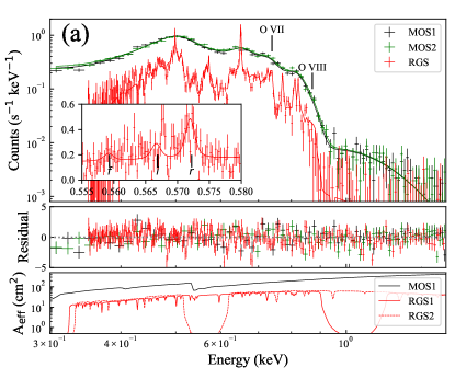
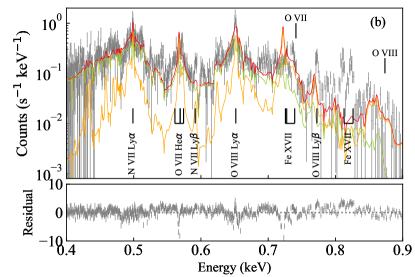
The X-ray spectra of the two MOS and the combined RGS data are shown in Figure 1. We characterize them by constructing a phenomenological spectral model for later use in physically-motivated models. For all the models in this work, we included the attenuation by the Galactic interstellar medium (ISM) in the direction of CAL87 and the ISM in the LMC using two photoelectric absorption models (tbabs and tbvarabs: Wilms et al., 2000). The column density of the former () was fixed at 7.581020 cm-2 (Dickey & Lockman, 1990) and that of the latter () was derived from the fitting. The metal abundance for the LMC absorption was fixed to be half of the Galactic ISM value (Russell & Dopita, 1992; Welty et al., 1999).
The continuum model was constrained using the MOS spectra with the richer statistics (Fig. 1 a). The spectra are characterized by a sharp cut-off at 0.7–0.9 keV despite the monotonically increasing effective area of the telescope. We thus used a single blackbody model with a photoelectric absorption by the O VII and O VIII K shell edges at 0.74 and 0.87 keV, respectively. The same model was used in the previous work using X-ray CCD spectra (Asai et al., 1998; Ebisawa et al., 2001). The bolometric luminosity corrected for the interstellar absorption () is erg s-1 assuming the spherical emission.
| Parameter | Value | |
|---|---|---|
| Galactic absorption | ( cm-2) | 0.758 (fix) |
| LMC absorption | ( cm-2) | 3.61 |
| Blackbody | (eV) | 80.1 |
| Norm. () | ||
| Edge energy | (keV) | 0.885 |
| (keV) | 0.743 | |
| Absorption edge depth | 2.59 | |
| 1.22 | ||
| Luminosity | ( erg s-1) | |
| (dof) | 1.20 (1744) | |
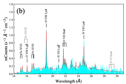
Upon the best-fit continuum model, we added line components by using both the MOS and RGS (Fig. 1 b). A handful of emission lines were identified in the RGS spectrum. We used Gaussian models for each line. From the best-fit energies, we identified emission lines of O VIII Ly and Ly, O VII He, N VII Ly and Ly, and four Fe XVII lines for the transition to the ground state (2s)2(2p)6 from the excited states shown in Table 2. All of them are electric dipole transitions of a large oscillator strength among the Fe XVII lines (Chen et al., 2003). These identifications are reported in Ebisawa et al. (2010).
| Label | Upper levelaafootnotemark: | Energy | bbWeighted oscillator strength. | ccEmissivity for the collisionally ionized plasma at a temperature of 0.6 keV (Smith et al., 2001). |
|---|---|---|---|---|
| (keV) | (cm3 s-1) | |||
| 3C | (2s)2(2p)5(3d)1 | 0.826 | 2.49 | 1.810-15 |
| 3D | (2s)2(2p)5(3d)1 | 0.812 | 0.64 | 0.610-15 |
| 3F | (2s)2(2p)5(3s)1 | 0.738 | 0.10 | 1.110-15 |
| 3G | (2s)2(2p)5(3s)1 | 0.726 | 0.13 | 1.510-15 |
Lower level is the ground state (2s)2(2p)6 for all.
Based on the line identifications, we fitted individual line complexes in a narrow (20–30 eV) energy range. For each of the Ly and Ly line complexes, we included two lines ( and ). The relative energy and intensity ratio between the two lines were fixed. The line intensity, energy shift, and broadening were fitted collectively. For the He line complex, we modeled with three lines of resonance (), inter-combination (), and forbidden (). For the Fe XVII line complex at 0.73–0.74 keV, we modeled with two lines (3F and 3G; Table 2). For the Fe XVII line complex at 0.81–0.83 keV, we modeled with two lines (3C and 3D; Table 2). The relative energy of each line was fixed. The line energy shift and broadening were fitted collectively, while the line intensity was fitted individually.
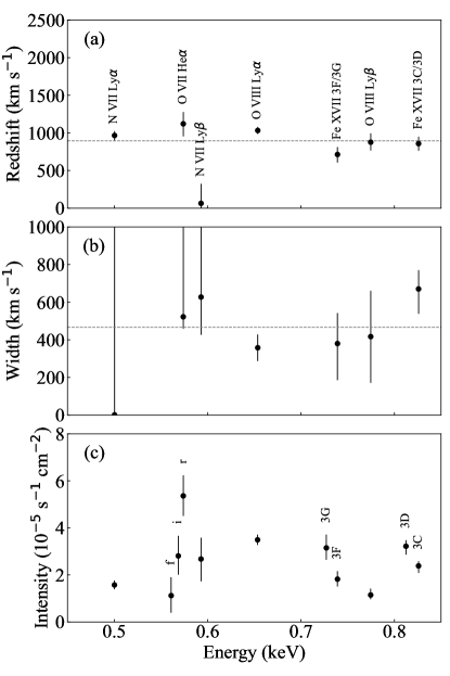
The result of the line complex fitting is shown in Figure 2. For the line shift and broadening, most complexes exhibit a redward shift with a mean of 900 km s-1 and broadening of 400 km s-1, which have been reported in Orio et al. (2004) and Ribeiro et al. (2014). The line shift of N VII Ly deviates from the trend, which may be biased by the RGS chip gap eliminating a large fraction of the line profile.
3 Model
3.1 Assumptions
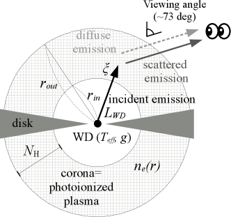
We assume a static and spherically-symmetric geometry (Fig. 3), in which a point-like source (WD) at the center is surrounded by the photoionized plasma (corona). The WD has an effective temperature of , a surface gravity of , and a luminosity of . It emits incident photons that photo-ionize the corona. It is assumed that the observer does not directly observe the incident emission from the WD being fully blocked by the disk but does observe the diffuse emission from the corona and the scattered emission originating in the WD. The inner and outer radii of the corona are and , respectively. The electron density profile is assumed to be . The metal abundance in the corona was fixed to 0.5 times the solar value (Wilms et al., 2000). The abundance would be determined from the data after a successful spectral modeling but is left out of scope for this study.
3.2 Analytical estimation
We first estimate the values of the model parameters analytically. The ionization parameter of the corona at is given by
| (1) |
in the unit of erg s-1 cm. This is almost constant throughout the corona due to the assumed radial dependence of . The electron column density in the line of sight is
| (2) |
The electron scattering optical depth is given by
| (3) |
in which cm2 is the Thomson cross-section. We make the hydrogen and electron column densities equal as . Finally, the observed luminosity is approximated as
| (4) |
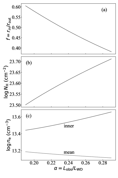
We now substitute erg s-1 (Table 1), cm from the partial eclipse in the X-ray light curve (Ebisawa et al., 2001), and erg s-1 cm from the observed lines, which we will derive later using a numerical calculation in § 3.3.1. The unknown variable is parameterized by , in which . As a function of , we solve the other unknown variables , , and normalized by as (Fig. 4). The set of equations solves only for a limited range of , and the derived values of the others are limited to a narrow range of – cm-3 and 0.38–0.61. Within this range, 0.21–0.34 and – cm-2.
The WD effective area and gravity are related to the luminosity erg s-1 as
| (5) |
and
| (6) |
respectively. Here, and are the radius and mass of the WD, respectively, and and are the Stefan-Boltzmann and gravity constants. For , cm from the mass-to-radius relation (Nauenberg, 1972), which corresponds to 0.2 . Then, kK and .
Some of these derived values can be verified by other relations not used above. First, the intrinsic luminosity is consistent with the luminosity to support steady nuclear burning on the WD surface of a mass of (Ebisawa et al., 2001). Second, if the observed energy shift of 900 km s-1 represents the radial velocity of the expanding corona:
| (7) |
in which is the wind mass loss rate and is the proton mass. By substituting yr-1 (Ablimit & Li, 2015), we obtain cm-1, which agrees with the value derived from equation (1) within an order.
3.3 Numerical calculation
We next verify that the analytically estimated parameters of the model (§ 3.2) are consistent with the numerical calculation of the photo-ionization plasma. We model the corona using the 1D radiative transfer code xstar v2.58e (Kallman et al., 2004). The code solves the radiative transfer in the scheme using the two-stream (radially inward and outward directions) solver and the escape probability approximation. It calculates the ionization/recombination, excitation/de-excitation, and heating/cooling balance at each zone of the spherically symmetric plasma and generates the charge state distributions and the level populations at each zone as well as synthesized X-ray spectra inward and outward of the plasma.
The heating and cooling sources are only the radiations. The heating source, or the incident emission, is given by the spectral energy distribution (SED) and the intensity parameterized with . The plasma is described by its density profile and total thickness (). The turbulent velocity is fixed to 400 km s-1 (§ 2.3). We left H and He at the solar metacility and C, N, O, Ne, Mg, Si, S, Ar, Ca, and Fe at a half solar value. We ignored other elements. The electrons have a Maxwellian energy distribution of a temperature () for the NLTE condition, which is calculated to reach a thermal balance between the heating and cooling.
For the purpose of a qualitative assessment, we use nearly a slab geometry of a uniform density and a blackbody spectrum for the incident emission using the best-fit values in the phenomenological model (§ 2.3). We use the code in an open geometry, in which the emission from the photoionized plasma can escape both the inward and outward directions, and the effects of radiative excitation are taken into account. The radiative excitation is known to be important for X-ray spectra from photoionized plasmas without the incident emission in the beam such as in Seyfert 2 galaxies (e.g., Kinkhabwala et al., 2002), which should also apply to the accretion disk coronae of X-ray binaries.
3.3.1 Presence and absence of lines
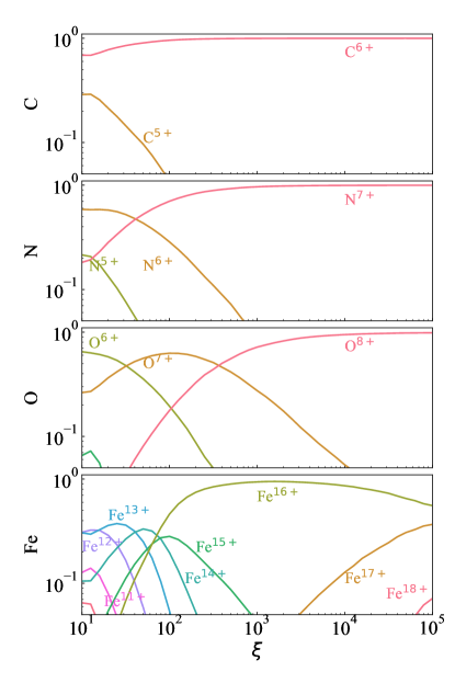
We first confirm the presence or absence of several lines expected at particular ionization states (Fig. 1b), which gives a constraint on the charge state distribution and the ionization parameter . Using parameters in the conceivable range as cm-2 and cm-3, we calculated the fraction of ionization states of C, N, O, and Fe averaged over the corona volume (Fig. 5). In the observed spectrum (Fig. 1b), we identified N VII lines (Ly and Ly) but not N VI lines (He) produced by the recombination cascade respectively of N7+ and N6+ ions; these conditions give the lower ionization limit . For O, we identified both O VIII (Ly and Ly) and O VII features (He) produced in the same process of O8+ and O7+ ions; these conditions in contrast gives the upper-lmit . Over this range, most Fe stays in the Ne-like (Fe16+), which is consistent with the presence of Fe XVII features produced by radiative decay from excited levels to the ground state of Fe16+ ions. The absence of Fe XVI and Fe XVIII features is due to the small fraction of Fe15+ and Fe17+ ions, respectively. These conditions are consistent with the estimated range of .
3.3.2 Line ratios
We next examine the intensity ratio of the identified lines. A well-established method is to use the He triplet line intensity ratios of O VII, namely the resonance (), inter-combination (), and forbidden lines (). and ratios are often used as temperature and density indicators when collisional processes dominate (Gabriel & Jordan, 1969) or the ionization and column density indicators when radiative processes dominate (Porter & Ferland, 2007). We refrain from using these diagnostics to constrain model parameters, though, given the poor constraints by the data (Fig. 1a inset). We only argue that it is reasonable to have the line to be the strongest and the line to be the weakest. The reasons for the former are that (1) MK from the thermal balance is close to the maximum formation temperature of the line in the collisional process and (2) the line is enhanced by the continuum pumping in the radiative process (Chakraborty et al., 2021). The reason for the latter is that cm-3 (§ 3.2) is much higher than the critical density of cm-3 for O (Blumenthal et al., 1972).
4 Physical Modeling
Based on the comparison of the observed spectra (§ 2.3) against the analytical (§ 3.2) and numerical (§ 3.3) calculations, we have verified that our assumed model and the parameterization are appropriate. We have also constrained the range of parameters. In order to contain the parameters more accurately, we now construct physical models using two complementary methods: one is 1D two-steam solver (xstar; § 4.1) and the other is 3D Monte Carlo solver (MONACO; § 4.2) of the radiative transfer in the corona.
4.1 1D two-stream solver
4.1.1 Setup
For the corona model, we use xstar in the same setup with § 3.3 except for two improvements; inclusion of the density profile and use of a WD atmosphere model spectrum for the incident emission. For the atmosphere model, we used TMAP (Rauch et al., 2010), which provides spectra111The data are available at http://astro.uni-tuebingen.de/~rauch/TMAF/flux_HHeCNONeMgSiS_gen.html. at 10—8000 Å for 405–1050 kK and (cm s-2)9 with varying abundances for major elements.
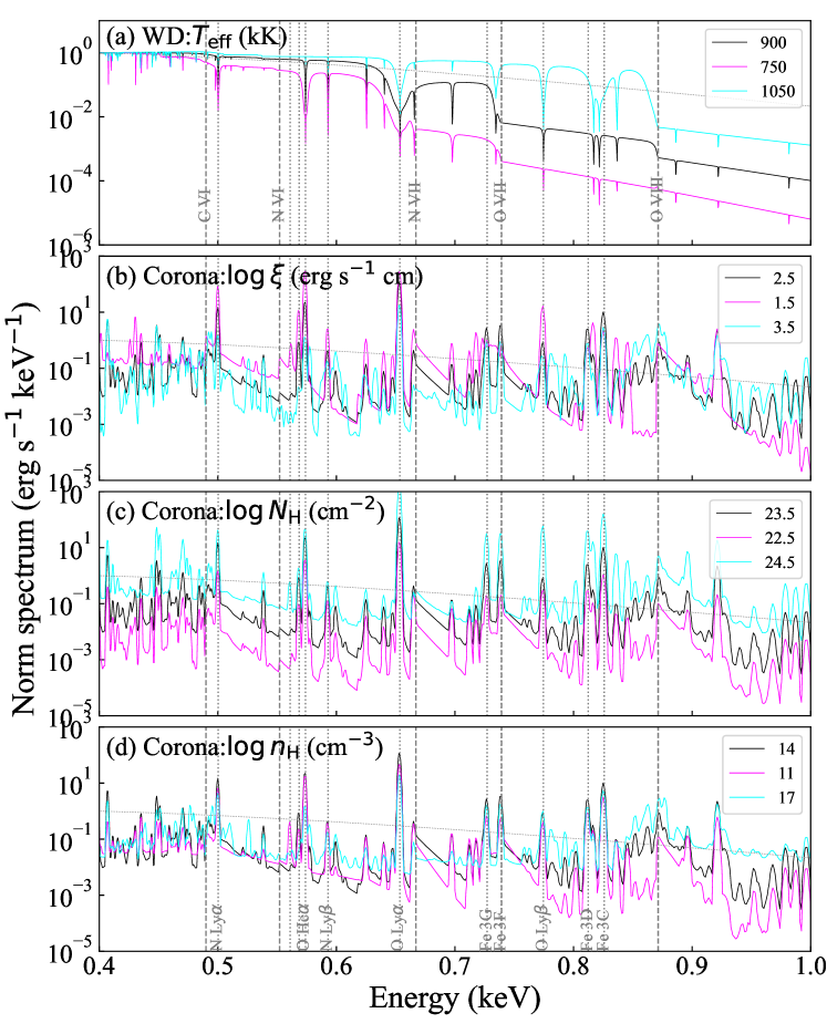
Figure 6 shows the synthesized spectra for different (a) atmosphere and (b–d) corona model parameters. Note that the incident emission for the corona model (b–d) is a featureless blackbody emission to clarify the corona effects, so they should be considered a transfer function. For , the most conspicuous changes are found in the O VII and O VIII edges. Their depth ratio is sensitive to . The edges, however, are insignificant in the corona transfer function in (b–d) as they are overwhelmed by the radiative recombination continuum emission. For , the charge state distribution changes significantly (Fig. 5) and, resultantly, the emission line ratio of different charge states; e.g., O VIII Ly and O VII He. For , the emission line ratios are not influenced, but the spectral shape above the edge energies change due to different columns in the line of sight. For , the O VII triplet changes most significantly (§ 3.3.2).
4.1.2 Result
We ran the xstar calculations for a grid of three parameters: , , and . We skip as the constraining power of the O VII triplet in the data is poor. The Galactic and Magellanic interstellar absorption columns were fixed to the value derived in the phenomenological fitting in Table 1. The turbulent velocity is fixed to 400 km s-1 (§ 2.3). The redshift () was fitted collectively. All the other parameters, including , are derived from the free parameter values based on the equations in § 3.2.
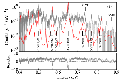
Figure 7 (a) shows the best-fit model and the residuals to the fit. The fitting is very poor. The best-fit parameters are away from those in the analytical estimates (§ 3). We identify several major discrepancies: emission lines are too strong, continuum emission is too weak, and the line profiles and ratios are poorly reproduced. Many of these are expected due to the known limitations of this solver, which we will discuss in § 5.
4.2 3D Monte Carlo solver
4.2.1 Setup
We next use the other radiative transfer code MONACO based on the Monte Carlo solver. MONACO is a photon tracking simulator based on the Monte Carlo framework (Watanabe et al., 2006a; Odaka et al., 2011a; Odaka, 2012) and is applied to many astrophysical applications (e.g., Hagino et al. 2015; Tomaru et al. 2018; Tanimoto et al. 2019; Mizumoto et al. 2021). We used MONACO version 1.7 release candidate and the database version 1.7.
A number of photons are emitted from the source and individual photons are tracked for their interactions with the matter placed in a 3D space. Each photon is tracked until it either escapes from the system or is destructed inside the system by absorption. Interactions between the photons and matter are calculated, including radiative excitation/de-excitation, ionization/recombination, photoelectric absorption, and scattering by free and bound electrons. However, because the framework is based on photon tracking, emission processes initiated by electrons such as free-free emission, are currently not included. We collected photons that experienced at least one interaction in the corona for the secondary emission, which includes both the scattered and diffuse emission.
The design of the framework allows one to calculate electron scattering in a 3D space in a consistent manner. The code does not calculate the thermal, ionization, and excitation balances unlike xstar. The electron density and temperature ( and ) as well as the charge state distributions of ions at each location need to be given as inputs. We used the result of the xstar simulation with the best-fit parameters (§ 4.1).
In the current version, MONACO calculates the level populations determined purely by the collisional processes based on the given and . This is not correct for the photo-ionized plasmas, in which the radiative processes also contribute. Unlike SKIRT version 9.0, a widely used Monte Carlo solver (Vander Meulen et al., 2023), MONACO calculates the photon-ion interactions for the H-like and He-like ions of major metals. For this work, we made two modifications to the code and the database: (1) inclusion of lower ionized Fe ions than Fe24+ down to Fe16+ and (2) recording both the positive and the negative deposit energy for the resonance scattering.
4.2.2 Result
We used the same approach with the 1D two-stream solver (§ 4.1) for the fitting. The geometry (Fig. 3) is set up in a 3D space. The simulation was run at the same grid of the same free parameters (, , and ) with the turbulent velocity fixed, the bulk velocity collectively fitted, other corona parameters derived from the grid parameters based on the analytical relations (§ 3.2), and the Magellanic and Galactic absorption fixed to the value from the phenomenological fitting.
For each grid parameter, we launched half a million photons from a point source at the center. The photons have a direction selected randomly over a uniform distribution and an energy selected randomly over a uniform distribution in 0.35–1.24 keV. The output was convolved with the input SED. For the grid of , , and kK as an example, (a) 4% photons are destructed in the corona by photo-electric absorption, (b) 72% photons escape from the system with no interactions, and (c) the rest escape with some interactions in the corona. We use (c) for the scattered plus diffuse emission.
Figure 7 (b) shows the best-fit model and the residuals to the fit. The fitting has improved with the best-fit parameters of , , and kK. They are in reasonable agreement with the analytical solution, yet the fitting is still too poor to derive their uncertainties. Some discrepancies remain, in particular, in the line profile of O VIII Ly, the line ratio within O VII He, and Fe XVII lines. We will discuss these issues in § 5.
5 Discussion
We constructed the spectral models of the corona based on two different solvers of the radiative transfer calculation and compared them to the observed spectra (§ 4). The xstar model yielded a poor fitting with the best-fit parameters far from those by the analytical estimates (§ 3.2). The MONACO model yielded a better fitting with the best-fit parameters consistent with the analytical estimates (§ 3.2). Both of them exhibited some discrepancies against the observations. We discuss possible reasons for four major discrepancies (§ 5.1–§ 5.4) and present the final fitting by considering the model limitations (§ 5.5).
5.1 Continuum emission
A major discrepancy in the xstar fitting (Fig. 7 a) is too weak continuum emission in the model. This makes sense considering that most of the continuum emission comes from the scattered emission by electrons in the corona, not the diffuse emission. In the 1D calculation of xstar, the electron scattering is implemented as a pure continuum absorption, and no scattered emission is produced.
In MONACO, the electron scattering is considered as scattering, including multiple scattering in the 3D space. We decompose the MONACO model spectrum into the scattered and diffuse components (Fig. 7 b). A single photon cannot be attributable to either one of them; a photon can experience both electron scattering and resonance scattering before escaping from the system. Here, the resonance scattering is not scattering but is absorption immediately followed by emission, thus should be included in the diffuse component. We divided all the photons based on their last interactions in the system. As expected, the scattered emission accounts for a large part of the continuum emission.
5.2 Line intensity
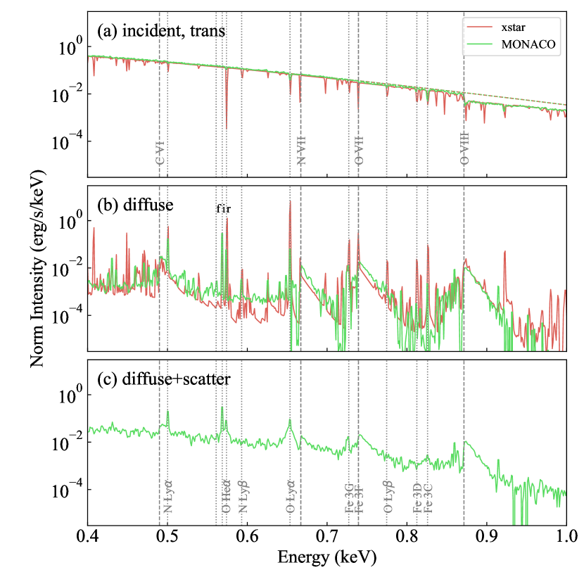
Another discrepancy in the xstar fitting (Fig. 7a) is the too strong line emission. The lack of scattered emission in the model accounts for this partially, but not fully. To illustrate this, we compare the xstar and MONACO spectra for the same parameters in Figure 8. For the transmitted spectra in panel (a), the continuum levels agree well between the two. For the diffuse spectra in panel (b), the radiative recombination continua at C VI, N VII, O VII, and O VIII agree in general. However, the line emission is systematically stronger for xstar than MONACO.
We argue two possibilities for the difference between the two solvers. One is that MONACO assumes that all excitation occurs only collisionally and does not include radiative excitation, which is known to enhance the emission lines (Chakraborty et al., 2021). The other is the assumption on the escape probability employed in xstar. The escape probability is an assumption necessary to solve the radiative transfer equations in reasonable computational resources in two-stream solvers, in which line photons escape from the system at a probability of . Here, is the opacity in the direction of the photon with a frequency of . It has been claimed that solvers based on the escape probability assumption yield line emission stronger than the accelerated lambda iteration solver, which is considered more reliable for the lines (Hubeny, 2001). In fact, Dumont et al. (2003) argued that the escape probability method yields an overestimation of the line intensity, in particular for resonance lines like O VIII Ly in optically thick cases, by an order.
5.3 Line profile
The opacity at the line center is very large for the conspicuous lines. Taking the strongest line O VIII Ly as an example, it is estimated by
| (8) |
in which , is the energy of the line, is the weighted oscillator strength, is the oxygen abundance relative to hydrogen, is the charge fraction of O8+, is the level population fraction of the ground state, is the Oxygen atomic mass, is the plasma temperature, and other symbols follow their conventions. For eV, , cm-2, , (Fig. 5), , and K, we obtain .
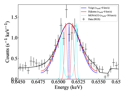
Line photons scatter numerous times locally due to their large opacity at the line center until their wavelength diffuses into the dumping wing of the line profile. Then, the photons escape from the system in a single long flight with a significantly reduced opacity. This is a premise for the escape probability approximation implemented in xstar. In such a situation, the line profile is known to be double-peaked around the center. The analytical solution is obtained for a plane-parallel (Harrington, 1973; Neufeld, 1991) and spherical (Dijkstra et al., 2006) geometry of a uniform density. Despite the premise, xstar synthesizes emission lines with the Voigt profile as it is computationally challenging to calculate the diffusion over wavelengths.
Figure 9 shows a close-up view of the O VIII Ly profile. The Voigt and Dijkstra profiles of no turbulence are shown with red and blue broken curves. They are smoothed with a Gaussian of the RGS energy resolution to compare to the data as shown with the solid curves of the same color. The smoothed Dijkstra profile matches better to the data than the smoothed Voigt profile. The turbulence velocity required in the phenomenological fitting (Fig. 2) can be explained by the line profile distortion by the radiative transfer effects. MONACO calculates the energy shift in every resonance scattering, thus the emergent line profile exhibits a distortion as shown with a cyan curve in Figure 2. This is too broad compared to the data, which we come back to later in § 5.5.
5.4 Line ratios
We discuss discrepancies found in several line ratios. First is the O VII He triplet. The line ratios are different between xstar and MONACO most notably in their synthesized diffuse spectra (Fig. 8 b). Among the resonance (), inter-combination (), and forbidden () lines, is the weakest in both models, which is expected (§ 3.3.2) and agrees with the observation (Fig. 1). However, the / ratio in the MONACO model is too strong compared to xstar and the observation. This stems from the limitation of MONACO, in which the level populations are calculated assuming that they are purely dominated by collisional processes. In the present application, both collisional and radiative processes matter, which are taken into account in the xstar calculation.
For the line ratios, we should focus on the xstar results. We examine the O VIII Lyman decrement (Ly/Ly). The observed decrement is 1/3 (Fig. 2), while the calculated value is 0.05 (Fig. 6). The observed Ly is too strong with respect to Ly. The calculated decrement hardly changes if we change the model parameters. Another line ratio discrepancy is found in the four Fe XVII lines (Fig. 7 a), in which the observed 3C/3D line pair is too strong with respect to the 3F/3G pair. Both are primarily due to the attenuation of incident photons beyond the O VII edge.
A possible solution would thus be to introduce another spectral component such as the collisionally ionized emission independent of the O VII edge attenuation. A plausible origin of the collisionally ionized plasma is the shock of the expanding shell. If we assume that it is produced by the shock of the expanding velocity of km s-1 (Fig. 2), the temperature is given by in which is the mean molecular weight, is the proton mass, and is the Boltzmann constant. Such a spectral component has been found in other SSS (Ness et al., 2022).
5.5 Final fitting
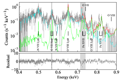
Based on the discussion above, we modify the spectral model for the final fitting. We start with the MONACO model (Fig. 7b) and add an apec model to account for the additional collisionally ionized plasma. We ignore the energy range of 0.565–0.569 and 0.715-0.740 keV to avoid the known caveats of the MONACO modeling for the O VII He () and Fe XVII 3F/3G lines. The plasma temperature () and the normalization of the apec model were fitted, while the abundance was fixed to half the solar value. Both the MONACO and apec models were red-shifted collectively. The result is given in Figure 10.
The fitting is finally good enough (reduced 1.5) to derive the best-fit parameter ranges as (erg s-1 cm) 2.52–2.55, (cm-2) 23.49–23.50, (kK) 1000–1005, (km s-1) 895–941, and (keV) 0.24–0.25. The corona model parameters agree well with the analytical solution. The O VIII Lyman decrement is now better reproduced since the Ly is contributed by the apec component. The Fe XVII 3C line is also reproduced by the apec model, which was not accounted for in the corona model only with MONACO. The O VIII Ly profile was better reproduced by a combination of the broad corona profile and the narrow collisionally ionized plasma profile. We still see some discrepancies such as Fe XVII 3D line at 0.81 keV and C VI radiative recombination continuum at 0.49 keV. These, along with the identified caveats and justification of the additional apec model, are left for future improvements of the codes.
6 Summary and Conclusion
We presented result of the spectral modeling of CAL87, a super-soft source dominated by emission features originating from the extended accretion disk corona around the WD. First, we presented a phenomenological fitting of the observed spectra with the EPIC-MOS and RGS instruments onboard XMM-Newton. Based on the fitting results and the system geometry, an analytical solution was obtained.
We then performed radiative transfer calculations using two codes employing different solvers and assumptions: xstar for a 1D, two-streamer solver and MONACO for a 3D, Monte Carlo solver. We fitted the spectral model to the data and identified discrepancies between the codes against the observation.
We discussed possible causes of these discrepancies in terms of the continuum emission, line intensity, line profile, and line ratio. We found that xstar excels in the level population calculations, while MONACO excels in the scattering (both electron and resonant line) calculations. We also argued for the presence of the additional collisionally ionized plasma. Finally, we presented the detailed spectral model that yields consistent parameters with the analytical model and agrees reasonably well with the observation.
In the coming microcalorimetry era in X-ray astronomy, the interpretation based on radiative transfer will be more seriously required than before. This is particularly the case for sources with hard X-ray spectrum dominated by reprocessed emission in the surrounding medium such as X-ray binaries during eclipse, accretion disk corona sources, and Seyfert 2 galaxies. Comparisons between different solvers and implementations, and comparisons against observations should be made in a wider range of applications than the one presented here.
References
- Ablimit & Li (2015) Ablimit, I., & Li, X. D. 2015, ApJ, 815, 17, doi: 10/gg66zw
- Arnaud (1996) Arnaud, K. A. 1996, in Astronomical Data Analysis Software and Systems V, ed. G. Jacoby & J. Barnes, Vol. 101, 17, doi: 1996ASPC..101…17A
- Asai et al. (1998) Asai, K., Dotani, T., Nagase, F., et al. 1998, ApJ, 503, L143, doi: 10.1086/311547
- Blumenthal et al. (1972) Blumenthal, G. R., Drake, G. W. F., & Tucker, W. H. 1972, ApJ, 172, 205, doi: 10/bp763z
- Callanan et al. (1989) Callanan, P. J., Machin, G., Naylor, T., & Charles, P. A. 1989, MNRAS, 241, 37P, doi: 10/gg66zt
- Chakraborty et al. (2021) Chakraborty, P., Ferland, G. J., Chatzikos, M., Guzmán, F., & Su, Y. 2021, ApJ, 912, 26, doi: 10.3847/1538-4357/abed4a
- Chen et al. (2003) Chen, G.-X., Pradhan, A. K., & Eissner, W. 2003, J. Phys. B, 36, 453, doi: 10.1088/0953-4075/36/3/305
- Cowley et al. (1990) Cowley, A. P., Schmidtke, P. C., Crampton, D., & Hutchings, J. B. 1990, ApJ, 350, 288, doi: 10.1086/168381
- Den Herder et al. (2001) Den Herder, J. W., Brinkman, A. C., Kahn, S. M., et al. 2001, A&A, 365, L7, doi: 10.1051/0004-6361:20000058
- Dickey & Lockman (1990) Dickey, J. M., & Lockman, F. J. 1990, ARA&A, 28, 215, doi: 10.1146/annurev.aa.28.090190.001243
- Dijkstra et al. (2006) Dijkstra, M., Haiman, Z., & Spaans, M. 2006, ApJ, 649, 14, doi: 10.1086/506243
- Dumont et al. (2003) Dumont, A.-M., Collin, S., Paletou, F., et al. 2003, A&A, 407, 13, doi: 10.1051/0004-6361:20030890
- Ebisawa et al. (2010) Ebisawa, K., Rauch, T., & Takei, D. 2010, AN, 331, 152, doi: 10.1002/asna.200911317
- Ebisawa et al. (2001) Ebisawa, K., Mukai, K., Kotani, T., et al. 2001, ApJ, 550, 1007, doi: 10/fs5dj6
- Gabriel & Jordan (1969) Gabriel, A. H., & Jordan, C. 1969, MNRAS, 145, 241, doi: 10.1093/mnras/145.2.241
- Greiner (1996) Greiner, J. 1996, Supersoft X-Ray Sources: Proceedings of the International Workshop Held in Garching, Germany, 28 February – 1 March 1996 (Berlin ; New York: Springer)
- Greiner et al. (2004) Greiner, J., Iyudin, A., Jimenez-Garate, M., et al. 2004, IAU Colloquium
- Hagino et al. (2015) Hagino, K., Odaka, H., Done, C., et al. 2015, MNRAS, 446, 663, doi: 10.1093/mnras/stu2095
- Harrington (1973) Harrington, J. P. 1973, MNRAS, 162, 43, doi: 10.1093/mnras/162.1.43
- Hubeny (2001) Hubeny, I. 2001, in Astronomical Society of the Pacific Conference Series, Vol. 247, Spectroscopic Challenges of Photoionized Plasmas, ed. G. Ferland & D. W. Savin, 197
- Jansen et al. (2001) Jansen, F., Lumb, D., Altieri, B., et al. 2001, A&A, 365, L1, doi: 10.1051/0004-6361:20000036
- Kallman et al. (2004) Kallman, T. R., Palmeri, P., Bautista, M. A., Mendoza, C., & Krolik, J. H. 2004, ApJS, 155, 675, doi: 10.1086/424039
- Kinkhabwala et al. (2002) Kinkhabwala, A., Sako, M., Behar, E., et al. 2002, ApJ, 575, 732, doi: 10.1086/341482
- Lanz et al. (2005) Lanz, T., Telis, G. A., Audard, M., et al. 2005, ApJ, 619, 517, doi: 10/ds5t3z
- Long et al. (1981) Long, K. S., Helfand, D. J., & Grabelsky, D. A. 1981, ApJ, 248, 925, doi: 10.1086/159222
- Macri et al. (2006) Macri, L. M., Stanek, K. Z., Bersier, D., Greenhill, L. J., & Reid, M. J. 2006, ApJ, 652, 1133, doi: 10.1086/508530
- Mizumoto et al. (2021) Mizumoto, M., Nomura, M., Done, C., Ohsuga, K., & Odaka, H. 2021, MNRAS, 503, 1442, doi: 10.1093/mnras/staa3282
- Nauenberg (1972) Nauenberg, M. 1972, ApJ, 175, 417, doi: 10/b5dqnq
- Ness et al. (2013) Ness, J.-U., Osborne, J. P., Henze, M., et al. 2013, A&A, 559, A50, doi: 10.1051/0004-6361/201322415
- Ness et al. (2022) Ness, J.-U., Beardmore, A. P., Bezak, P., et al. 2022, A&A, 658, A169, doi: 10.1051/0004-6361/202142037
- Neufeld (1991) Neufeld, D. A. 1991, ApJ, 370, L85, doi: 10.1086/185983
- Odaka (2012) Odaka, H. 2012, PhD thesis, The University of Tokyo
- Odaka et al. (2011a) Odaka, H., Aharonian, F., Watanabe, S., et al. 2011a, ApJ, 740, 103, doi: 10/b8k462
- Odaka et al. (2011b) —. 2011b, ApJ, 740, 103, doi: 10.1088/0004-637X/740/2/103
- Orio et al. (2004) Orio, M., Ebisawa, K., Heise, J., & Hartmann, W. 2004, RMA&A, 20, 210, doi: 10.1017/s025292110015256x
- Paerels et al. (2001) Paerels, F., Rasmussen, A. P., Hartmann, H. W., et al. 2001, A&A, 365, L308, doi: 10.1051/0004-6361:20000069
- Pakull et al. (1988) Pakull, M. W., Beuermann, K., van der Klis, M., & van Paradijs, J. 1988, A&AL, 203, L27
- Porter & Ferland (2007) Porter, R. L., & Ferland, G. J. 2007, ApJ, 664, 586, doi: 10.1086/518882
- Rauch et al. (2010) Rauch, T., Orio, M., Gonzales-Riestra, R., et al. 2010, ApJ, 717, 363, doi: 10.1088/0004-637X/717/1/363
- Ribeiro et al. (2014) Ribeiro, T., Lopes De Oliveira, R., & Borges, B. W. 2014, ApJ, 792, 20, doi: 10.1088/0004-637x/792/1/20
- Russell & Dopita (1992) Russell, S. C., & Dopita, M. A. 1992, ApJ, 384, 508, doi: 10.1086/170893
- Sala et al. (2008) Sala, G., Hernanz, M., Ferri, C., & Greiner, J. 2008, ApJ, 675, L93, doi: 10.1086/533530
- Sala et al. (2010) —. 2010, ApJ, 331, 201, doi: 10.1002/asna.200911327
- Schandl et al. (1997) Schandl, S., Meyer-Hofmeister, E., & Meyer, F. 1997, A&A, 80, 73
- Schmidtke et al. (1993) Schmidtke, P. C., McGrath, T. K., Cowley, A. P., & Frattare, L. M. 1993, PASP, 105, 863, doi: 10.1086/133246
- Smith et al. (2001) Smith, R. K., Brickhouse, N. S., Liedahl, D. A., & Raymond, J. C. 2001, ApJ, 556, L91, doi: 10/cgpdmx
- Tanimoto et al. (2019) Tanimoto, A., Ueda, Y., Odaka, H., et al. 2019, ApJ, 877, 95, doi: 10/grmq2q
- Tomaru et al. (2018) Tomaru, R., Done, C., Odaka, H., Watanabe, S., & Takahashi, T. 2018, MNRAS, 476, 1776, doi: 10/gdh4vh
- Turner et al. (2001) Turner, M. J., Abbey, A., Arnaud, M., et al. 2001, A&A, 365, L27, doi: 10/dnvdbt
- van Rossum & Ness (2010) van Rossum, D. R., & Ness, J. U. 2010, AN, 331, 175, doi: 10/bwgbsd
- Vander Meulen et al. (2023) Vander Meulen, B., Camps, P., Stalevski, M., & Baes, M. 2023, A&A, 674, A123, doi: 10.1051/0004-6361/202245783
- Watanabe et al. (2006a) Watanabe, S., Sako, M., Ishida, M., et al. 2006a, ApJ, 651, 421, doi: 10/c4n9vb
- Watanabe et al. (2006b) —. 2006b, ApJ, 651, 421, doi: 10.1086/507458
- Welty et al. (1999) Welty, D. E., Frisch, P. C., Sonneborn, G., & York, D. G. 1999, ApJ, 512, 636, doi: 10.1086/306795
- Wilms et al. (2000) Wilms, J., Allen, A., & McCray, R. 2000, ApJ, 542, 914, doi: 10.1086/317016