[a,b]Jon-Ivar Skullerud
Spectral properties of bottomonium at high temperature: a systematic investigation
Abstract
We investigate spectral features of bottomonium at high temperature, in particular the thermal mass shift and width of ground state S-wave and P-wave state. We employ and compare a range of methods for determining these features from lattice NRQCD correlators, including direct correlator analyses (multi-exponential fits and moments of spectral functions), linear methods (Backus-Gilbert, Tikhonov and HLT methods), and Bayesian methods for spectral function reconstruction (MEM and BR). We comment on the reliability and limitations of the various methods.
1 Introduction
An important task in QCD phenomenology is to determine the spectral functions of hadronic and current–current correlators. These encode physical information about inter alia the existence and properties of bound states and resonances, transport properties, and multiparticle thresholds. The spectral functions are related to the euclidean correlators computable on the lattice by an integral transform, but computing the spectral function given a finite set of noisy correlator data is known to be an ill-posed problem. Numerous methods have been developed to attempt to handle this problem (see [1, 2] for recent reviews), which all have their inherent limitations. The purpose of the study that is reported here is to obtain a better understanding of a subset of these methods by applying them to a specific problem, namely determining the temperature dependence of the mass and width of the 1S and 1P bottomonium states computed in lattice non-relativistic QCD (NRQCD).
The bottomonium system has been studied in lattice NRQCD for a long time [3, 4, 5, 6, 7, 8]. The NRQCD approach has the benefit of a simple spectral representation with a temperature-independent kernel,
| (1) |
Since the heavy quark is not in thermal equilibrium, the full range of points are available for the spectral reconstruction. Finally, since at least the state is expected to survive as a bound state up to quite high temperatures, the peak position and thermal width remain well-defined quantities which can be used to benchmark the methods.
2 Lattice setup
Our simulations are carried out using anisotropic lattices with an improved gauge action and an improved Wilson fermion action with stout smearing, following the parameter tuning and ensembles generated by the Hadron Spectrum Collaboration [13, 14]. The results presented here were produced using the “Gen2L” ensembles, which have active quark flavours with MeV and an approximately physical strange quark. The spatial lattice spacing is fm and the anisotropy . The temperature is given by and is varied by changing the number of sites in the temporal direction. For more details about the ensembles, see Ref. [15, 16] and references therein.
| 128 | 64 | 56 | 48 | 40 | 36 | 32 | 28 | 24 | 20 | 16 | 12 | |
| (MeV) | 47 | 95 | 109 | 127 | 152 | 169 | 190 | 217 | 253 | 304 | 380 | 507 |
| 0.28 | 0.57 | 0.65 | 0.76 | 0.91 | 1.01 | 1.14 | 1.30 | 1.52 | 1.82 | 2.28 | 3.03 |
The quarks were simulated using an NRQCD action including and leading spin-dependent corrections, with mean-field improved tree-level coefficients [4].
3 Time-derivative moments
The idea behind the moments method is to consider the correlator in (1) as the integral of a weighted spectral function . The temporal derivatives of the correlator are then the moments of , and the salient features of , such as the locations and widths of its peaks, and hence those of , can be inferred from these derivatives.
If is approximated by a sum of Gaussians,
| (2) | ||||
| we find | ||||
| (3) | ||||
| (4) | ||||
| (5) | ||||
where can be approximated by a constant if . Specifically, from (5) we see that the ground state width can be extracted in the large- limit assuming the same condition holds, while the first derivative (4) can be used to determine the ground state mass.
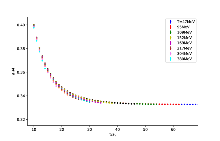
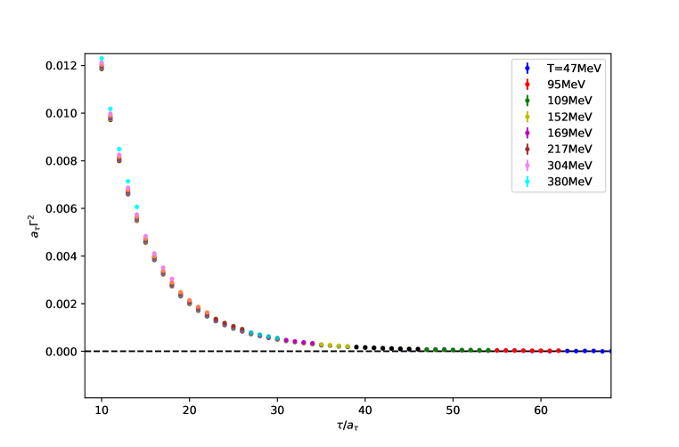
The results for the vector () channel are shown in fig. 1. We see that both the first and second log-derivative approach a plateau at large . To determine the mass and width, the log-derivatives are fitted to a simplified version of (4,5),
| (6) |
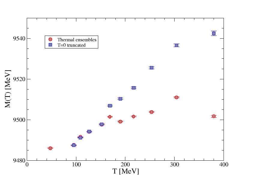
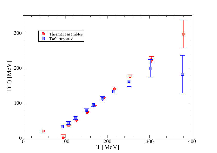
The results for and for (1S) are shown in fig. 2 as a function of temperature (red points). At first sight, both and appear to increase with temperature. However, this increase may in part be an effect of the shorter temporal range available at higher temperatures, where and have not yet reached a plateau at the maximum value of . To disentangle this from real, thermal effects, the same analysis has been carried out on the ensemble (which may be considered to be at ), with the temporal range restricted to . The results of this are shown by the blue points in fig. 2. We see that there are no substantial thermal effects for MeV. Above this temperature, the mass from the thermal ensemble lies below that from the corresponding truncated analysis, while the thermal width appears to be increasing from zero at MeV (albeit still consisten with zero within errors). For further details about the method and results, see [11].
4 Linear methods
All the linear methods considered here (Tikhonov [17], Backus–Gilbert [18], and HLT [19]) regularise the inverse problem by avoiding a pointwise estimate of and instead constructing a “smeared” spectral function,
| (7) |
where the smearing kernel plays the role of a finite-width approximation to . It may in turn be expressed as a linear combination of the NRQCD kernel functions,
| (8) |
where are coefficients which encode the location of the sampling point and are determined by the method. Inserting (8) into (7) and using the spectral definition of the correlator (1) then yields
| (9) |
The coefficients are determined by minimising a functional , where the three methods differ by their choices for these functionals:
| Tikhonov: | (10) | ||||||
| BG: | (11) | ||||||
| HLT: | (12) |
and is a gaussian with width centred on . An important distinction between HLT and the other two is that in HLT, the smearing width is an input parameter, while in the other two methods the smearing kernel and hence its width is entirely determined by the data and the hyperparameter . The stability of the results with respect to variations in is an important consideration with these methods.
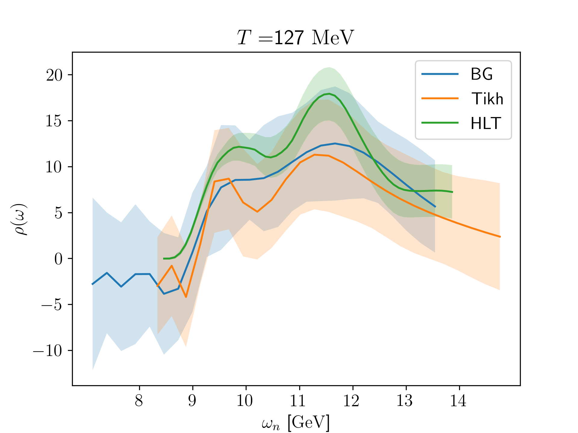
Results for the spectral functions from the three methods are shown in the left panel of fig. 3. We see that the results from all three methods are consistent, but that HLT yields a considerably more well-determined spectral function than the other two, as can be seen from the width of the respective error bands.
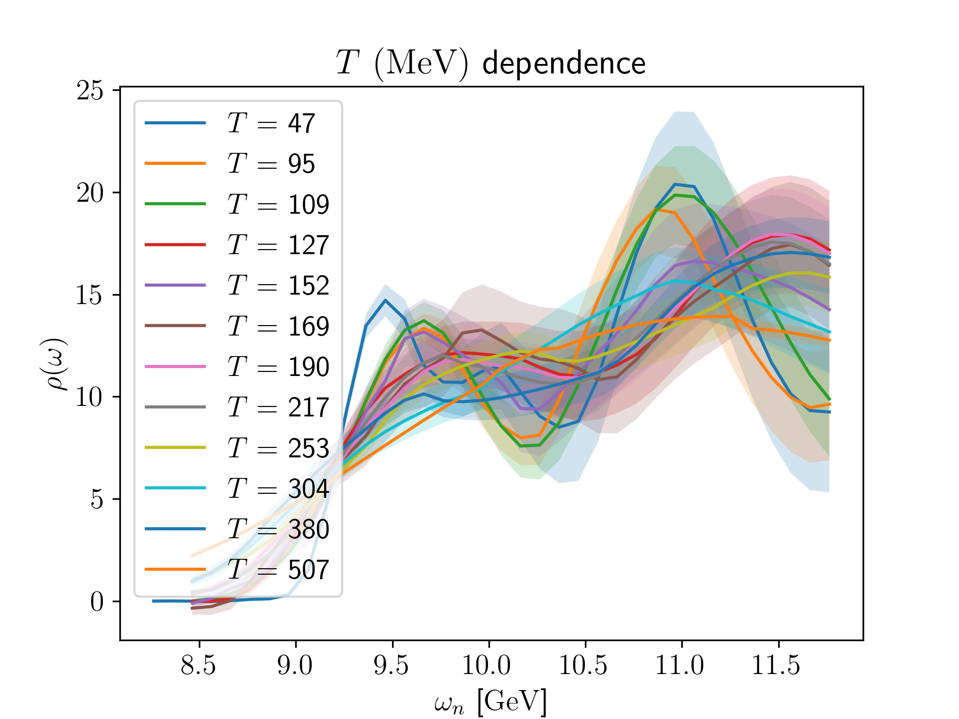
In the right panel of fig. 3 we show the spectral functions from the HLT method at all temperatures. We see a progressive broadening and apparent positive mass shift as the temperature is increased. However, in light of the discussion in the previous section, in the absence of an equivalent analysis on the zero-temperature ensemble, we are not yet in a position to draw any firm conclusion on this. For more details about the methods and results, see [10].
5 Bayesian methods
Bayesian methods, including the maximum entropy method (MEM) [20] and the BR method [21], regulate the inverse problem by introducing prior information, such that the probability of the spectral function given the data and the prior information is given by
| (13) |
where is the standard likelihood () and parametrises the prior probability . is written in terms of a default model which is the most likely spectral function in the absence of data. The main difference between MEM and BR lies in the form for ,
| (14) |
The two methods also differ in that in the usual (Bryan) implementation of MEM, is restricted to the singular subspace of the kernel ( in the case of NRQCD), while BR constructs the solution from the full -dimensional space.
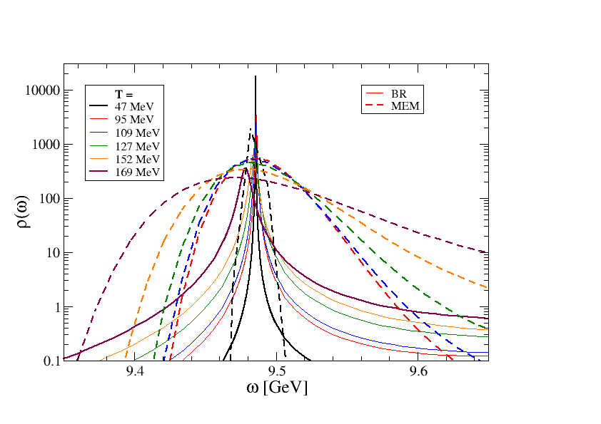
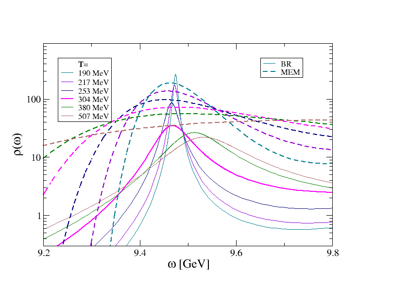
In fig. 4 we compare the results from MEM and BR for the spectral function in the vicinity of the (1S) peak. With both methods we see that the peak shifts to the left and broadens as the temperature increases. However, the quantitative differences are significant: MEM consistently gives a larger width than BR, and the shift in the peak position also tends to be larger in the MEM results.
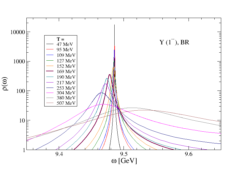
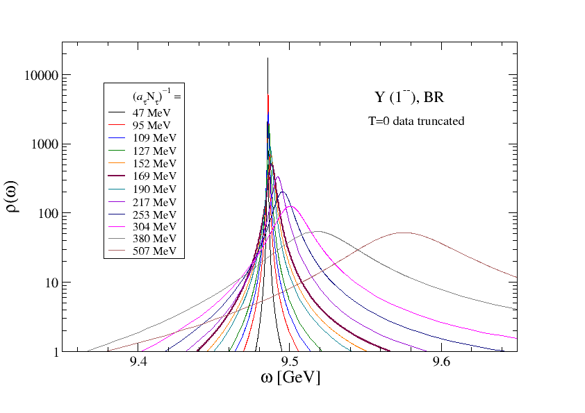
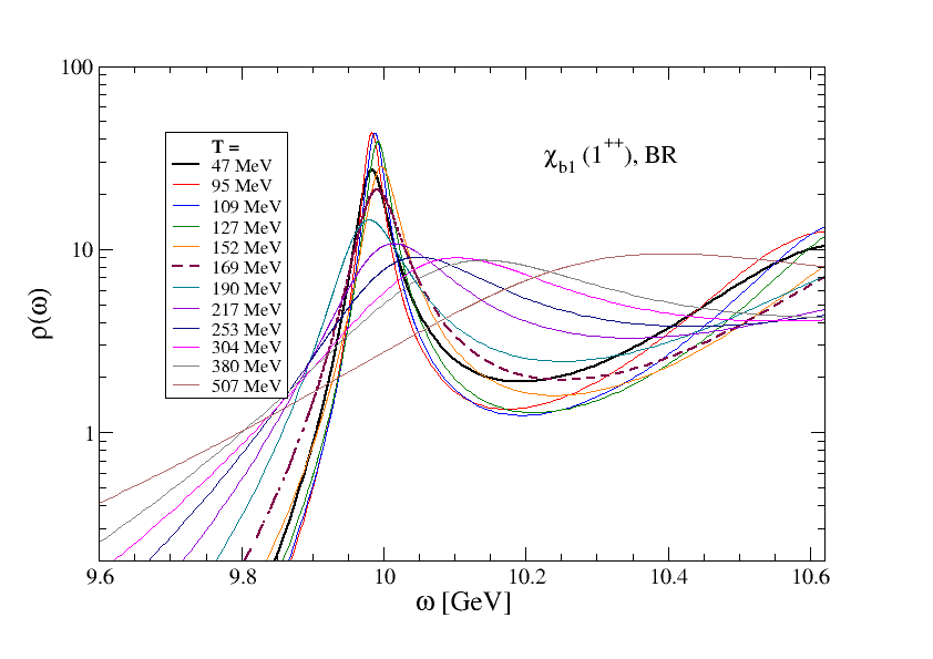
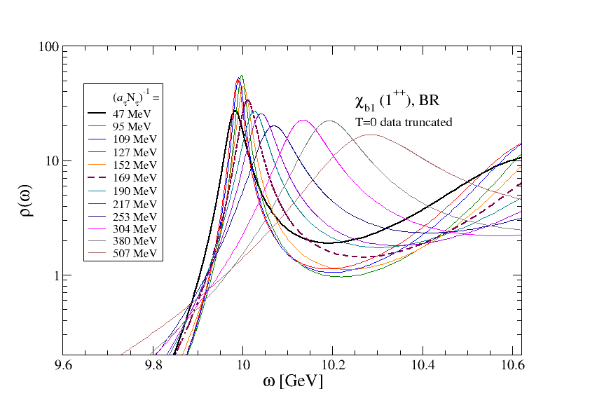
Fig. 5 shows spectral functions from the BR method for the and at all temperatures. The left hand plots show the results from the thermal ensembles, while the right hand plots show results from the equivalent analysis on the zero-temperature ensemble. We see that the zero-temperature control always gives a positive shift in the peak position and a broadening. It is only when the thermal results differ from the control that a real thermal effect can be concluded. In this case we can infer thermal effects in both channels; in particular, for the , comparing the thermal and control results we can infer a negative mass shift as well as a thermal broadening, while the thermal results on their own would suggest a positive mass shift.
6 Discussion
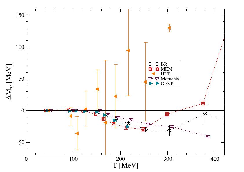
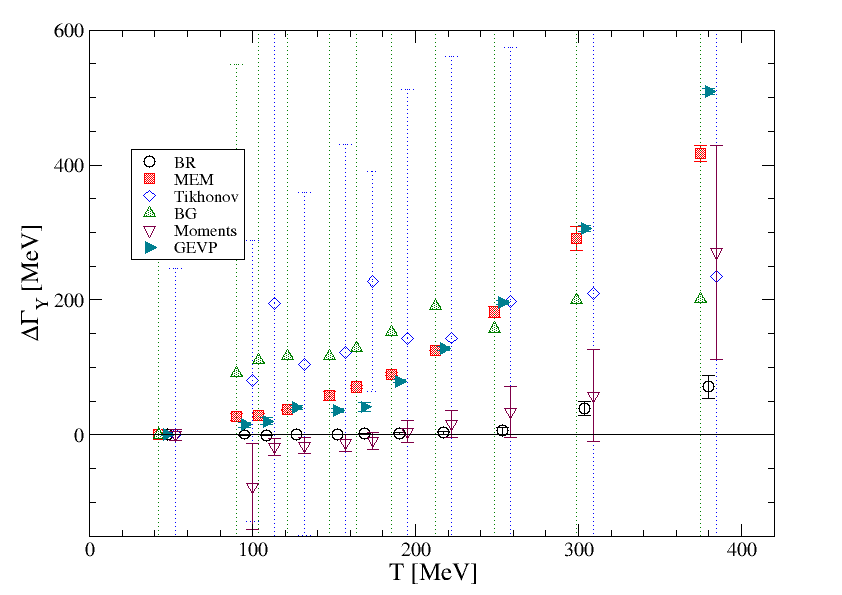
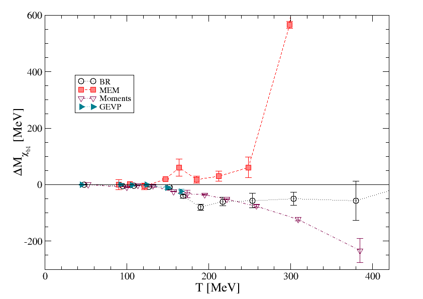
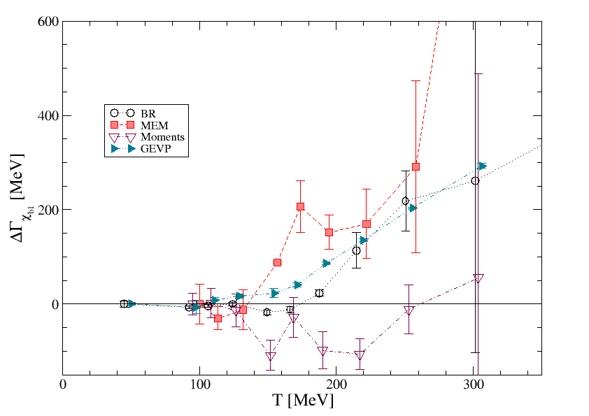
Fig. 6 shows the results for the thermal mass shift and thermal width of the and for all the methods discussed here. In addition, we show results from the use of a generalised eigenvalue problem (GEVP) [12], where masses are determined from standard exponential fits to the resulting optimised correlators, while the widths are determined by applying the time-derivative moments methods to the same correlators.
The mass shifts and thermal widths in fig. 6 are obtained by subtracting the zero-temperature mass and width ,
| (15) |
For the moments and BR methods, and are determined from the truncated zero-temperature correlators (control data) as described in section 3. This prescription attempts to correct for the main finite- effects, but it should be noted that it may be complicated by the presence of excited states at low which are not resolved in an analysis of the truncated data and may not be present in the thermal correlators. Further analysis will be necessary to disentange any such effects.
For the other methods (MEM, linear methods, GEVP) the ordinary analysis at the lowest temperature has been used to determine . We expect the masses obtained from the GEVP method to be relatively insensitive to finite- artefacts, while the GEVP widths come from the moments method applied to the GEVP projected correlators and so may have similar artefacts. We expect the MEM and the linear methods to have a reduced and when the full control analysis is carried out. In all cases, uncertainties include both statistical and systematic uncertainties.
The first thing to note is that the linear methods have much larger uncertainties than the others. This is not surprising, as the width of the smearing kernel in these methods is in most cases larger than the physical width of the states under consideration. The Tikhonov and BG results for the mass are too noisy to be shown. In HLT the width is an input parameter and can therefore not be used as an estimator (or upper bound) for the physical width.
With these provisos, we see an encouraging qualitative and, in some cases, even quantitative agreement between the different methods. Notably, there is agreement between BR, MEM, moments and GEVP about a small negative mass shift of up to 40 MeV for the (1S), for 150 MeV250 MeV. A similar mass shift may be seen in the (1P), using BR, moments and GEVP. The current MEM analysis does not show this shift, but the effect may be obscured by the finite , as observed with the BR method in fig. 5.
Concerning the width, there is rough agreement (within large uncertainties) for the , but for the there is a discrepancy, with BR and moments giving a much smaller width (MeV at MeV) than the other methods. Although the full zero-temperature control analysis may change this, the GEVP method should be less sensitive to this, so this discrepancy needs to be studied further.
7 Summary and outlook
We have studied the mass and width of ground state S- and P-wave bottomonium ( and ) with a range of different methods. We find agreement between correlator and Bayesian methods on a negative mass shift of up to 20–40 MeV at MeV, as well as qualitative agreement on the mass and width of . There is a discrepancy for the width of , which requires further investigation. Linear methods (Tikhonov, Backus–Gilbert, HLT) have intrinsically larger uncertainties when applied to this particular problem, but their results are consistent with those of the other methods.
Our results suggest that it is feasible to determine spectral features at high temperature by comparing results using different methods. A crucial part of understanding the systematics is the zero-temperature control analysis (see also [22, 5]). Applying this to all methods is currently in progress. The procedure outlined here may also be extended to study excited states [12], or to transport properties, where the balance of strengths and limitations of the different methods may be different.
Data and software
The gauge ensembles were produced using openqcd-fastsum [23]; information about the ensembles can be found at [24]. The NRQCD correlators were produced using the FASTNRQCD package [25]. We anticipate making the full dataset and scripts for the results presented here available after a future publication.
Acknowledgments
We acknowledge EuroHPC Joint Undertaking for awarding the project EHPC-EXT-2023E01-010 access to LUMI-C, Finland. This work used the DiRAC Data Intensive service (DIaL2 and DIaL) at the University of Leicester, managed by the University of Leicester Research Computing Service on behalf of the STFC DiRAC HPC Facility (www.dirac.ac.uk). The DiRAC service at Leicester was funded by BEIS, UKRI and STFC capital funding and STFC operations grants. This work used the DiRAC Extreme Scaling service (Tesseract) at the University of Edinburgh, managed by the Edinburgh Parallel Computing Centre on behalf of the STFC DiRAC HPC Facility (www.dirac.ac.uk). The DiRAC service at Edinburgh was funded by BEIS, UKRI and STFC capital funding and STFC operations grants. DiRAC is part of the UKRI Digital Research Infrastructure. This work was performed using the PRACE Marconi-KNL resources hosted by CINECA, Italy. We acknowledge the support of the Supercomputing Wales project, which is part-funded by the European Regional Development Fund (ERDF) via Welsh Government, and the University of Southern Denmark for use of computing facilities. This work is supported by STFC grant ST/X000648/1 and The Royal Society Newton International Fellowship. RB acknowledges support from a Science Foundation Ireland Frontiers for the Future Project award with grant number SFI-21/FFP-P/10186. RHD acknowledges support from Taighde Éireann – Research Ireland under Grant number GOIPG/2024/3507.
References
- [1] A. Rothkopf, Inverse problems, real-time dynamics and lattice simulations, EPJ Web Conf. 274 (2022) 01004 [2211.10680].
- [2] W. Jay, Approaches to the inverse problem, PoS LATTICE2024 (2025) 002.
- [3] G. Aarts, C. Allton, S. Kim, M.P. Lombardo, M.B. Oktay et al., What happens to the and in the quark-gluon plasma? Bottomonium spectral functions from lattice QCD, JHEP 1111 (2011) 103 [1109.4496].
- [4] G. Aarts, C. Allton, T. Harris, S. Kim, M.P. Lombardo et al., The bottomonium spectrum at finite temperature from Nf = 2 + 1 lattice QCD, JHEP 1407 (2014) 097 [1402.6210].
- [5] S. Kim, P. Petreczky and A. Rothkopf, Quarkonium in-medium properties from realistic lattice NRQCD, JHEP 11 (2018) 088 [1808.08781].
- [6] R. Larsen, S. Meinel, S. Mukherjee and P. Petreczky, Thermal broadening of bottomonia: Lattice nonrelativistic QCD with extended operators, Phys. Rev. D 100 (2019) 074506 [1908.08437].
- [7] R. Larsen, S. Meinel, S. Mukherjee and P. Petreczky, Excited bottomonia in quark-gluon plasma from lattice QCD, Phys. Lett. B 800 (2020) 135119 [1910.07374].
- [8] H.T. Ding, W.P. Huang, R. Larsen, S. Meinel, S. Mukherjee, P. Petreczky et al., In-medium bottomonium properties from lattice NRQCD calculations with extended meson operators, 2501.11257.
- [9] T. Spriggs et al., A comparison of spectral reconstruction methods applied to non-zero temperature NRQCD meson correlation functions, EPJ Web Conf. 258 (2022) 05011 [2112.04201].
- [10] A. Smecca et al., The NRQCD spectrum at non-zero temperatures using Backus-Gilbert regularisations, PoS LATTICE2024 (2025) 197 [2502.03060].
- [11] R.H. D’arcy et al., NRQCD bottomonium at non-zero temperature using time-derivative moments, PoS LATTICE2024 (2025) 203 [2502.03951].
- [12] R. Bignell et al., Anisotropic excited bottomonia from a basis of smeared operators, PoS LATTICE2024 (2025) 202 [2502.03185].
- [13] R.G. Edwards, B. Joó and H.-W. Lin, Tuning for three-flavors of anisotropic clover fermions with stout-link smearing, Phys.Rev. D78 (2008) 054501 [0803.3960].
- [14] Hadron Spectrum Collaboration collaboration, First results from 2+1 dynamical quark flavors on an anisotropic lattice: Light-hadron spectroscopy and setting the strange-quark mass, Phys.Rev. D79 (2009) 034502 [0810.3588].
- [15] G. Aarts et al., Properties of the QCD thermal transition with flavours of wilson quark, Phys. Rev. D 105 (2022) 034504 [2007.04188].
- [16] G. Aarts, C. Allton, R. Bignell, T.J. Burns, S.C. García-Mascaraque, S. Hands et al., Open charm mesons at nonzero temperature: results in the hadronic phase from lattice QCD, 2209.14681.
- [17] A.N. Tikhonov, On the stability of inverse problems, Proceedings of the USSR Academy of Sciences 39 (1943) 195.
- [18] G. Backus and F. Gilbert, The Resolving Power of Gross Earth Data, Geophysical Journal International 16 (1968) 169.
- [19] M. Hansen, A. Lupo and N. Tantalo, Extraction of spectral densities from lattice correlators, Phys. Rev. D 99 (2019) 094508 [1903.06476].
- [20] M. Asakawa, T. Hatsuda and Y. Nakahara, Maximum entropy analysis of the spectral functions in lattice QCD, Prog. Part. Nucl. Phys. 46 (2001) 459 [hep-lat/0011040].
- [21] Y. Burnier and A. Rothkopf, Bayesian approach to spectral function reconstruction for euclidean quantum field theories, Phys.Rev.Lett. 111 (2013) 182003 [1307.6106].
- [22] A. Kelly, A. Rothkopf and J.-I. Skullerud, Bayesian study of relativistic open and hidden charm in anisotropic lattice QCD, Phys. Rev. D97 (2018) 114509 [1802.00667].
- [23] J.R. Glesaaen and B. Jäger, openQCD-FASTSUM, Apr., 2018. 10.5281/zenodo.2216355.
- [24] G. Aarts, C. Allton, M.N. Anwar, R. Bignell, T.J. Burns, S. Chaves Garcia-Mascaraque et al., FASTSUM Generation 2L anisotropic thermal lattice QCD gauge ensembles, Jan., 2025. 10.5281/zenodo.10636046.
- [25] R. Bignell, S. Kim and D.K. Sinclair, FASTNRQCD: Non-relativistic QCD propagator and correlator code for bottomonium, Oct., 2024. https://gitlab.com/fastsum/NRQCD.