Spectral variability of FIRST bright QSOs with SDSS observations
Abstract
For some samples, it has been shown that spectra of QSOs with low redshift are bluer during their brighter phases. For the FIRST bright QSO sample, we assemble their spectra from SDSS DR7 to investigate variability between the spectra from White et al. (2000) and from the SDSS for a long rest-frame time-lag, up to 10 years. There are 312 radio loud QSOs and 232 radio quiet QSOs in this sample, up to . With two-epoch variation, it is found that spectra of half of the QSOs appear redder during their brighter phases. There is no obvious difference in slope variability between sub-samples of radio quiet and radio loud QSOs. This result implies that the presence of a radio jet does not affect the slope variability on 10-year timescales. The arithmetic composite difference spectrum for variable QSOs is steep at blueward of 2500Å. The variability for the region blueward of 2500 Å is different to that for the region redward of 2500 Å.
Subject headings:
galaxies: active –quasars: general – techniques: spectroscopic1. Introduction
Variability is a common phenomenon in Active Galactic Nuclei (AGNs) and QSOs, from X-ray to radio wavelengths, on timescales from hours to decades (e.g., Huang et al. 1990; Mushotzky et al. 1993; Bian & Zhao 2003a; Breedt et al. 2010). Detection of variability is also a method to isolate QSO samples from photometric data (e.g., Rengstorf 2004; Wu et al. 2011). The origin of the small-amplitude and long-time-scale optical variability in AGN is still a question to debate, and there are several main models: accretion disc instabilities (e.g. Rees 1984; Kawaguchi et al. 1998), gravitational lensing (e.g. Hawkins 1996), and star/supernova activity (e.g. Cid Fernandes, Aretxaga & Terlevich 1996, Torricelli-Ciamponi et al. 2000), reprocessing of X-rays and reflection of optical light by the dust(e.g., Breedt et al. 2010). It is suggested that the predicted slopes of the structure function for QSOs variability are 0.83, 0.44, and 0.25 for supernovae in the starburst model, instabilities in the accretion disk, and microlensing, respectively (Kawaguchi et al. 1998; Hawkins 2002).
There are two main methods to investigate QSOs variability: one is from photometry, the other is from spectra. With the photometric method, many correlations are found between photometric variability and luminosity, rest-frame wavelength, redshift, time-lag, supermassive lack hole mass (SMBH mass), and Eddington ratio (e.g., Huang, et al. 1990; Hawkins 2002; Vanden Berk et al. 2004; de Vries et al. 2005; Bauer et al. 2009; Ai et al. 2010; Meusinger et al. 2011). Using the photometric data in various optical bands, the spectral variability can also be studied, suggesting that the QSOs would be bluer during their brighter phase (e.g., Giveon et al. 1999; Vanden Berk et al. 2004; de Vries et al. 2005; Meusinger et al. 2011; Gu & Ai 2011). With large QSO samples, increasing variability at shorter wavelengths supports accretion disk instability as the explanation for the structure function (e.g., Vanden Berk et al. 2004; de Vries et al. 2005; Bauer et al. 2009).
The advantage of the photometric method is that the photometric variability amplitude is accurate and that it takes less observing time compared with the spectroscopic method. However, it just monitors the flux variability in a few wavelength bands which usually have contributions from many components, including continuum and strong emission lines. In order to investigate the spectral variability in QSOs in more detail, the spectroscopy-based method is necessary. Wilhite et al. (2005) gave a sample of 315 significantly variable QSOs from multi-epoch spectroscopic observations of the SDSS. They found that the average difference spectrum (bright phase minus faint phase) is bluer than the average single-epoch QSO spectrum, also suggesting that QSOs are bluer when brighter (see also Meusinger et al. 2011). Pu et al. (2009) and Bian et al. (2010) also investigated spectral variability with data from the Palomer-Green (PG) QSOs spectrophotometrical monitoring projects for individual QSOs, but with many epochs (). They also found this result for all these individual QSOs. However, these objects are very nearby, with low redshifts. Their spectral slopes are influenced by their host galaxy contributions (e.g., Shen et al. 2011).
There is usually a change in the distribution of radio to optical flux ratio for QSO sample, at which the population can be divided into radio loud (RL) QSOs and radio quiet (RQ) QSOs, and its origin is still a question open to debate (e.g., White et al 2000; Jiang et al. 2008). It is suggested that the difference between RL and RQ QSOs is due to their SMBH masses, their SMBH spins, or Eddington ratios (e.g., Woo & Urry 2002; Ho 2002; Laor 2003; Bian & Zhao 2003b). It is interesting to investigate the spectral variation for RL QSOs and RQ QSOs. For the objects from the FIRST bright QSOs survey (White et al. 2000), we assembled their spectra from the Sloan Digital Sky Survey Data Release 7 (SDSS DR7; York et al. 2000; Abazajian et al. 2009) to investigate the variability between the spectra from White et al. (2000) and from the SDSS for a long rest-frame time-lag, up to 10 years. The slope variation is measured for the two epochs, as well as composite spectra to construct the ratio and difference spectra.
In Section 2, the sample and data are described.The spectroscopic data analysis is given in Section 3. Results and discussions are presented in section 4. Section 5 is our conclusion.
2. Sample and Data
2.1. The FBQS with SDSS spectra
With the FIRST survey and the Automated Plate Measuring Facility (APM) catalog of the Palomar Observatory Sky Survey I (POSS-I) plates, White et al. (2000) presented their FIRST Bright Quasar Survey (FBQS) catalog with 636 QSOs distributed over 2682 . There are four criteria to select FBQS candidates: radio-optical positional coincidence (1”.2); E 17.8; optical morphology (stellar-like); POSS color bluer than O-E=2. They do not find a bimodal distribution in radio to optical flux ratio, and the numbers of RQ/RL QSOs are comparable. Spectra for the FBQS were obtained at different observatories: the 3 m Shane telescope at Lick Observatory, the 2.1 m telescope at Kitt Peak National Observatory, the 3.5 m telescope at Apache Point Observatory,the Multiple Mirror Telescope (MMT), and the 10 m Keck II telescope. These FIRST spectra can be downloaded from the CDS 111http://cdsarc.u-strasbg.fr/viz-bin/Cat?J/ApJS/126/133.
The SDSS DR7 (York et al. 2000) contains imaging of almost 11663 and follow-up spectra for roughly galaxies and quasars. All observations were made at the Apache Point Observatory in New Mexico, using a dedicated 2.5m telescope. The SDSS spectra were obtained through 3” fibers. With these 636 FBQS, we cross-correlate them with the total SpecPhotoALL table 222http://cas.sdss.org/CasJobs/MyDB.aspx in the SDSS DR7. Applying the FBQS criterion of stellar-like morphology, we find 544 objects in SDSS DR7 spectral database with separations less than 1”, which is about 86% of 636 FBQSs. There are 312 RL QSOs and 232 RQ QSOs. Except for several objects, most of the FBQS objects have only one spectrum in the SDSS DR7 spectral database. For the SDSS spectra, the observational wavelength coverage is from 3800 to 9200Å. For spectra from White et al. (2000), the observational wavelength coverage can be found in their Table 1, which typically stops at a little shorter wavelength than the SDSS spectrum in the red part and starts a little longer than the SDSS spectrum in the blue part.
2.2. The subsample of spectrally variable QSOs

In order to isolate the spectrally variable QSOs from the total QSOs, we calculate the integrated relative flux change (). For the two-epoch spectra of a QSO, we calculate the mean flux () and the difference flux () at every wavelength (SDSS flux minus FIRST flux). This integrated relative flux change measures the total relative flux change between the two epochs over a large optical wavelength range, rather than the variation at just one wavelength or in one filter. With the stars to calibrate the QSO flux variability, Wilhite et al. (2005) found that the criterion for selecting spectrally variable QSOs is that the absolute value of the integrated is larger than 0.2-0.1 when the high-S/N epoch S/N is below 50. Here, we examine two-epoch spectra and find this criterion of 0.2 is appropriate to select the spectrally variable QSOs. In the left panel of Figure 1, we give the integrated relative flux change, , versus the integrated S/N from SDSS and the redshift. The total numbers of two-epoch measurements are 242 and 319 for RQ QSOs and RL QSOs. Considering the S/N in the ratio spectrum, we select QSOs with ratio spectral S/N greater than 5.0. There are 221 RQ QSOs and 269 RL QSOs ratio spectra meeting the criterion. For the subsample of variable QSOs, the two-epoch numbers are 142 (58%) for variable RQ QSOs, and 204 (64%) for variable RL QSOs. We define the convention that the SDSS spectrum is in the brighter phase and the relevant FIRST spectrum is in the fainter phase if is positive.
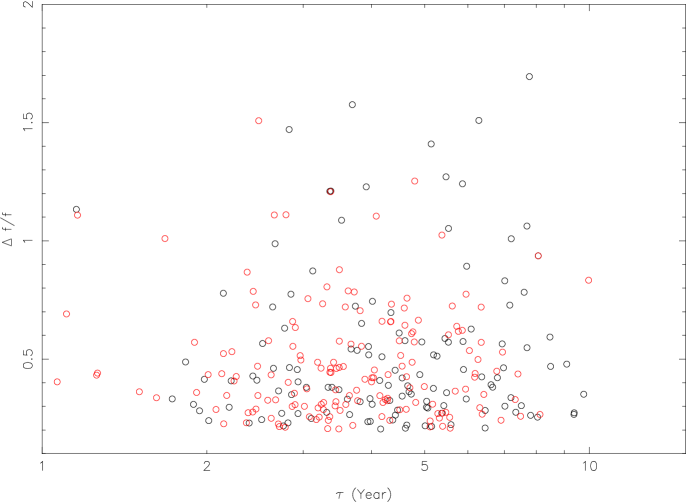
For our variable QSO sample, the rest-frame time-lag is from to years (right panel in Fig. 1), while the rest-frame time-lag is less than 1 year for Whihite et al. (their Fig. 7, 2005), less than 2 years for Vanden Berk et al. (2004). We calculate structure functions at three continuum wavelengths of 5100Å, 3000Å, and 1350Å. However, the data are so dispersed that we can’t give the slopes measurement of the structure functions. The right panel of Figure 1 is the integrated relative flux change versus the rest-frame time-lag. For the distribution of , K-S statistic is 0.081 with a signification level of 81%. Assuming that the RL and RQ QSOs were drawn from the same population, the probability that we would have observed a K-S statistics as at least as large as 0.081 is 81%. There is no obvious difference of for variable RL QSOs and RQ QSOs.
3. spectroscopic analysis
Our goal is to investigate the spectral variability from the two-epoch variation for the total QSO sample, as well as the sub-samples of RL and RQ QSOs. All the observed spectra are corrected for Galactic extinction using their values, assuming an extinction curve of Cardelli et al. (1989; IR band; UV band) and O’Donnell (1994; optical band) with . The correction for Galactic extinction has no effect on the slope variation calculation, however, it would have a large effect on the continuum flux, as well as the slope of the composite spectrum.
It is common to use the power law formula, () to approximately fit the QSO continuum spectrum. We use ”continuum windows” (in the rest frame), known to be relatively free from strong emission lines, of 1350-1370, 1450-1470, 1680-1720, 2200-2250, 3790-3810, 3920-3940, 4000-4050, 4200-4230, 5080-5100, 5600-5630, 5970-6000, 6005-6035, 6890-7010Å (Forster et al. 2001; Vanden Berk et al. 2001). Because of the pseudo-continuum from UV/optical Fe II (from 2200 to 3800 Å, from 4400 to 5500Å), the Balmer continuum (blueward of 4000Å), as well as the host contribution for low luminosity QSOs, there is some difficulty in finding the ideal ”continuum windows”. At the same time, for FBQS spectra from White et al. (2000), there are two obvious strong atmospheric absorptions around 6900 Å and 7600Å in the observational frame. These two regions are excluded in the fitting. Considering the errors in both coordinates, we use the linear regression algorithm, , to parameterize the power-law fit (Press et al. 1992, p. 660).
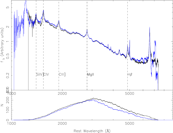
For most objects, we have one spectrum from SDSS, , one spectrum from FBQS of White et al. (2000), , as well as the ratio spectrum from SDSS/FBQS flux ratio, . With three power-law fits for three spectra, we can obtain three slopes, three intercepts and their errors. In the spectrum of the SDSS/FBQS flux ratio, the emission line contribution would vanish or be decreased (Wilhite et al. 2005). Therefore, the slope variation between the SDSS spectrum and the FBQS spectrum is adopted to be the power-law fit to their spectral flux ratio, rather than the slope difference from the direct SDSS and FBQS spectral fits (Figure 2).
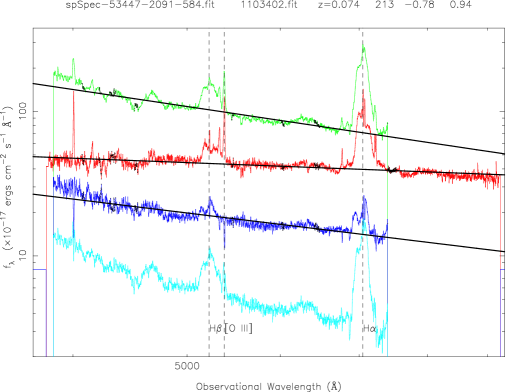
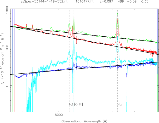
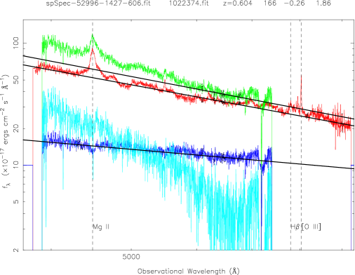
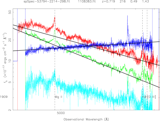

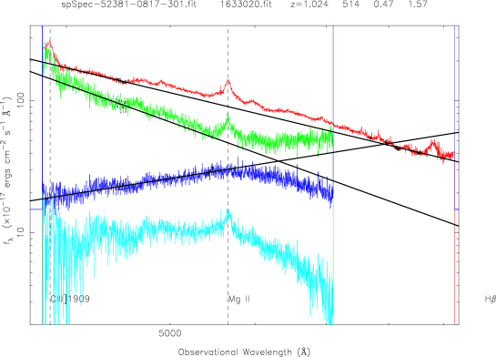
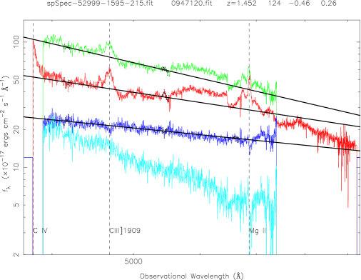
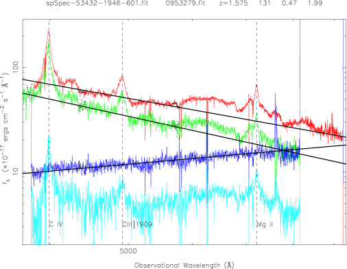
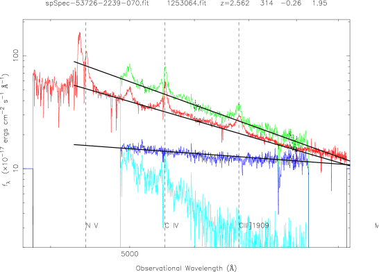
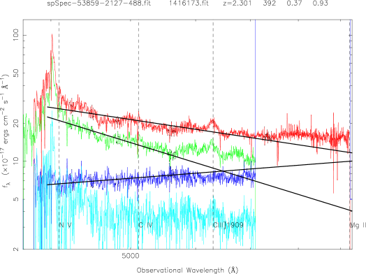
Figure 2 is an example showing QSOs two-epoch variability for 5 pairs of QSOs with different redshifts (from top to bottom, about 0.1, 0.6, 1.0, 1.5, 2.5). The red curve is for the SDSS spectrum, the green is for the FBQS spectrum from White et al. (2000); the blue curve is for the spectral flux ratio of the bright-phase spectrum to the faint-phase spectrum; the cyan cure is their different spectrum. The solid lines are the best linear fits at ”continuum windows” (black points) by . The left panels show the QSOs that become bluer during the brighter phase, while the right panels show another trend, i.e., redder during the brighter phase.
4. Results and Discussions
4.1. The distributions of spectral slope and slope variation
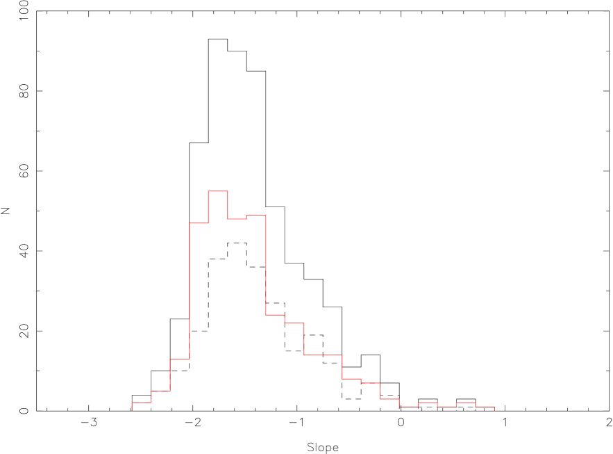
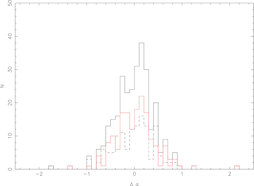
Figure 3 is the spectral slope distributions for SDSS QSOs (left panel) and the slope variation distribution (right panel). The mean of the slope distribution of SDSS QSOs is with a standard deviation of 0.59. It is , , respectively for RQ QSOs and RL QSOs from SDSS. In checking the spectra with the reddest slopes, it is found that these are mainly QSOs with obvious host galaxy contribution. For the slope variation distribution in the subsample of variable QSOs, the mean slope variation (the slope of brighter phase minus the slope of the fainter phase) is with a standard deviation of 0.42. It is , , respectively for variable RQ QSOs and RL QSOs.
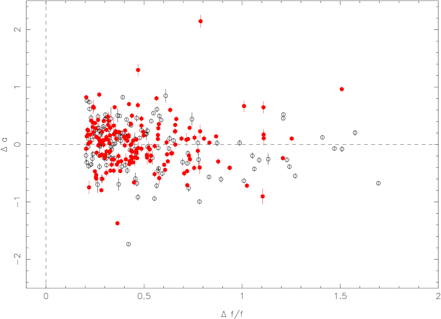
In Figure 4, we give the slope variation versus the integrated relative flux change for selected variable QSOs. About half QSOs get redder during their brighter phases. Selecting for larger than 1.0, this is still the case. For the distribution of , K-S statistic is 0.066 with a signification level of 90%. Assuming that the RL and RQ QSOs were drawn from the same population, the probability that we would have observed a K-S statistics as at least as large as 0.066 is 90%.
4.2. Relation between the slope variation and the continuum flux ratio
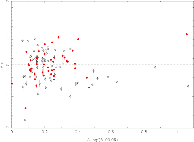
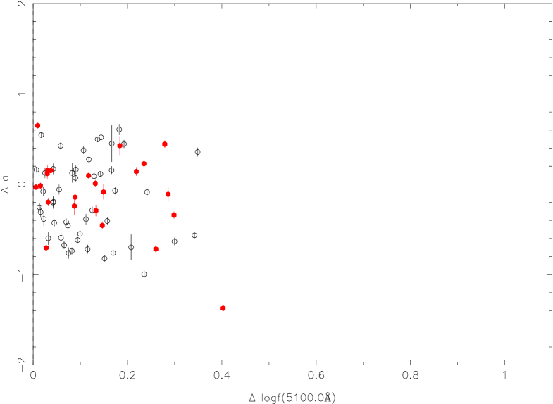
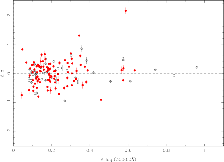
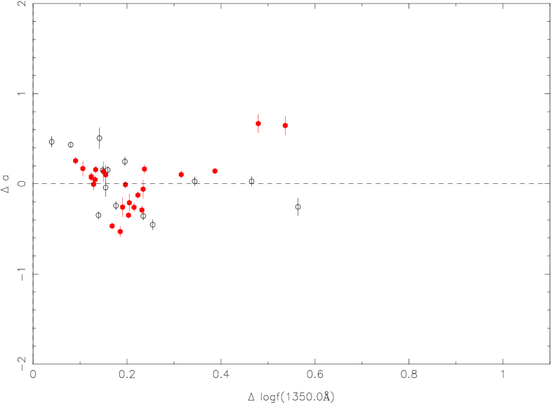
For the UV/optical spectrum, clean determinations of continuum fluxes are mainly at three wavelengths from 5100Å, 3000Å, and 1350Å, which are used in the mass calculation (et al., Shen et al. 2011). These three wavelengths of 5100Å, 3000Å, and 1350Å are selected to discuss the relationship between the slope variation and the continuum flux ratio. The continuum flux ratio is the flux at the brighter epoch divided by the flux at the fainter epoch at the specified rest wavelength. In order to exclude the limits of observed spectral range, we consider the slope variation at a wavelength of 5100Å for variable QSOs with , at a wavelength of 3000Å for variable QSOs with , and at a wavelength of 1350Å for variable QSOs with .
In Figure 5, we give the relation between the slope variation and the continuum flux ratio at 5100Å for low redshift selected variable QSOs () (top left, top right panel); at 3000 Å (, bottom left panel); at 1350 Å (, bottom right panel). For the top right panel, it is done for the [O iii] flux correction in FIRST spectra. We did not find strong correlations between the slope variation and the continuum flux ratio, the Spearman coefficients are -0.03, -0.07, -0.10, -0.25, and the probabilities of null hypothesis are 0.75, 0.55, 0.24, 0.14, respectively (Figure 5, from left to right and from top to bottom).
It is also clear that the slope variation of half the points is positive when the flux ratio is larger than zero in all different subsamples, i.e., about half of the objects become redder during their brighter phases. The red points are for RL QSOs and the black points are for RQ QSOs. In low redshift QSOs, the host would contribute in the observed object spectrum and make it complex (e.g., Shen et al. 2011). For the low luminosity QSO sub-sample ( ¡ erg s-1 ), it is still the case. The top right panel in Figure 5 is the same relation but with the recalibration for FIRST spectra from White et al. (2000) from the [O iii] 5007 flux (see section 4.4).
4.3. Composite ratio spectrum
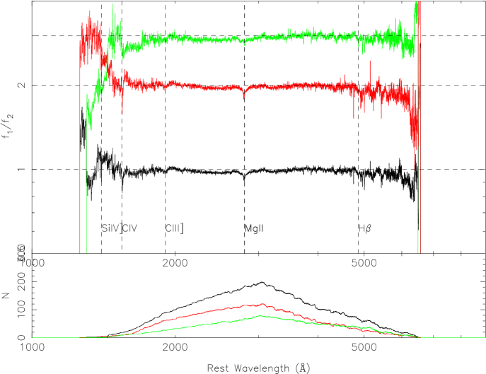
In order to clarify the average slope variability of RL and RQ QSOs, we calculate their composite ratio spectra. There are two methods to derive the composite spectrum, one is the median spectrum, which can preserve the relative fluxes of the emission lines; the other is the geometric mean spectrum, which can preserve the global continuum shape. In order to investigate the slope variation, we use the geometric mean spectrum, , where is the flux of spectrum number i at wavelength , and n is the total number of spectra contributing to the bin (e.g., Vanden Berk et al. 2001). In the left panel of Figure 6, the geometric composite spectra of our SDSS QSOs and FBQS QSOs are very consistent. Vanden Berk et al. (2001) suggested the best fitting windows in the composite spectrum are 1350-1365Å and 4200-4230Å. Using a power law function to fit the composite spectrum in the windows of 1450-1470Å and 4200-4320Å, we find that their slopes are for SDSS spectra and for FIRST spectra, which is a little larger than -1.56 by Vanden Berk et al. (2001) for a large sample of 2204 QSOs from SDSS.
Here we also use that approach to calculate the geometric composite spectrum for the flux ratio spectrum. The flux ratio is the ratio of the brighter phase spectrum to the fainter phase spectrum. All spectra of variable QSOs are scaled to the continuum flux at 3060Å. In the right panel of Figure 6, we show the geometric mean composite spectra for the flux ratio spectra for variable RL and RQ QSOs. The black curve is for all QSOs, the red curve is for RL QSOs, and the green one is for RQ QSOs. For clarity, the magnitudes are multiplied by 2 and 3 for RL and RQ QSOs. The geometric mean flux-ratio spectrum for RL QSOs is almost the same as that for RQ QSOs. All the geometric mean composite spectra are very flat. This is consistent with our results in Figures 3, 4, and 5, where about half of the objects have spectra becoming redder during their brighter phases.
For the slope variability for individual QSOs, we found that all the nearby PG QSOs in the sample of Kaspi et al. (2000; for the reverberation mapping technique) appear bluer during their brighter phases over multiple-epochs (Pu et al. 2006). However, when just considering two-epoch, it is not the case (see Fig. 1 in Pu et al. 2006). Using just two-epoch to investigate the slope variability for an entire ensemble of quasars, Wilhite et al. (2005) suggested that the QSOs continua are bluer when brighter. Here we directly calculate the slope variation for every object and find that almost half the objects appear redder continua when brighter. This paper uses the analysis framework developed in Pu et al.(2006) on a much bigger sample of QSOs. The advantages of the current sample are that it has a roughly equal fraction of RL and RQ objects, and that it contains a substantial sub-sample of objects that vary strongly in the optical/UV.
4.4. Difference of flux calibration between SDSS spectra and spectra from White et al.

The uncertainty of the slope variation is mainly due to the selection of ”continuum windows” in the power-law fitting. Its mean error is less than 0.1. For the continuum flux ratio, the uncertainty is mainly due to the different calibration of SDSS spectra and spectra from White et al. (2000). For SDSS spectra, with the calibration from non-variable stars, it is suggested that the flux correction between High-S/N to low-S/N is about 1.03-1.01 between 4000Å and 9000Å (Wilhite et al. 2005). In logarithm space, it is 0.004-0.01, or 0.01-0.025 mag. For the spectra from White et al. (2000), we use the flux of [O iii] 5007Å to estimate their flux uncertainties.
Considering that [O iii] 5007Å emission is coming from narrow line region (NLRs), spatially extended low-density regions, we assume that the [O iii] fluxes do not vary significantly over several year timescales and then normalize each FIRST spectrum to have the same [O iii] flux as the SDSS spectrum. Due to the blending of H with [O iii] , we use the following steps to calculate the [O iii] flux (see Hu et al. 2008 for details). The first step is subtraction of the power-law, Balmer continuum, and pseudo-continuum Fe ii emission. The second is the multi-Gaussian fit to the [O iii] 4959, 5007 Å doublet lines and Hermite-Gaussian for H . We excluded objects when the absorption in 6900Å and 7600Å is in the fitting region of [O iii] 5007Å and H . The measured flux ratio for [O iii] 5007Å is shown in Figure 7. The mean value of the [O iii] flux ratio in logarithm space is with a standard deviation of 0.23. It suggests that the SDSS flux calibration is consistent with that for FBQS but with a moderate dispersion.
In the top right panels in Figure 5, we show the slope variation versus the bright-to-faint flux ratio after considering the [O iii] 5007Å correction for the spectra from White et al. (2000). It maintains the result that almost half of the QSOs are not bluer during their bright phases. Of course, that correction can’t be used for higher redshift QSOs without observations of [O iii] 5007Å. In Figure 5, considering the continuum flux ratio larger than 0.23 from the [O iii] recalibration, a little more QSOs with z ¡ 0.7 tend to be bluer during brighter phases, and there is still half QSOs showing redder during brighter phases for QSOs with .
4.5. Composite spectrum and the composite difference spectrum
It is suggested that arithmetic and geometric mean composites have different properties (Vanden Berk et al. 2001). Because QSO spectra can be described by power laws, by the definition of geometric mean, the geometric mean can preserve the average power-law slope. The arithmetic mean can retain the relative strength of the non-power-law features, such as emission lines.
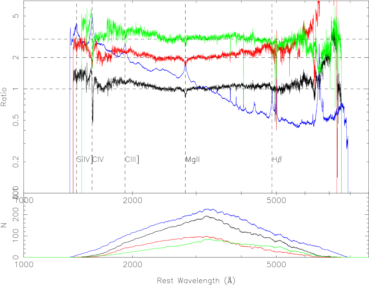
For the subsample of variable QSOs, the composite difference spectrum is calculated from the geometric/arithmetic mean for QSO spectra with flux scaled to 3060Å. For the difference spectra (brighter phase minus fainter phase), the geometric mean composite difference spectrum is almost the same as the geometric mean composite spectrum. However, with the arithmetic mean, they are different, with the slope of the arithmetic mean composite difference spectrum of and the slope of arithmetic composite spectrum of . The slope of -1.75 for the difference spectrum is larger than -2.0 by Wilhite et al. (2005).
In Figure 8, the blue curve is the arithmetic mean composite spectrum from the SDSS spectra scaled to a value of 1 at 3060Å. The ratio of the arithmetic mean composite difference spectrum to the arithmetic mean composite spectrum is shown as a black curve. Larger values of this ratio indicate a more variable portion of the spectrum. We can find smaller values in emission lines of C iv ,Mg ii ,H , etc on the ratio spectrum, showing that the emission lines are considerably less variable than the continuum. It is consistent with the intrinsic Baldwin effect for emission lines (Kinney et al. 90). For rest wavelengths greater than 2500 Å, the ratio is flat (near 1), showing that the composite difference spectrum has the same continuum slope as the composite spectrum. However, the values blueward of 2500 Å in the ratio spectrum become larger than 1. Vanden Berk et al. (2004) showed that the variability dependence appears to flatten around 3000 Å (see their Figure 13), which is consistent with the flatness in this dataset around 3000 Å.
The ratio spectrum from 2500 Å to 3600 Å is flat (near 1), showing that the composite difference spectra have the same continuum slope as the composite spectrum. Blueward of 2500 Å, the composite difference spectrum (brighter phase minus fainter phase) has more variance than the average QSO spectrum. Redward of 3600 Å, the variance becomes slightly greater than 1 and increases slowly toward longer wavelengths.
Since the ratio spectrum is flat excluding the region blueward of 2500 Å, the steep slope of the composite difference spectrum is due to the higher value blueward of 2500 Å, which also shows a difference in the composite spectra constructed from both the arithmetic and geometric means. The variability for the region blueward of 2500 Å is different from that for the region between 2500 Åand 3600 Å, and different from the region redward of 3600 Å.
Our interpretation of this result is that the lack of variability from 2500 Å to 3600 Å arises because this spectral region is dominated by Balmer continuum and Fe II emission. As pointed out above, the arithmetic mean is sensitive to spectral features. The Fe II region is composed of the many members of the stronger UV multiplets, and they may completely dominate the continuum emission (e.g., Wampler 1986). Since the emission lines in general are shown to vary less than the continuum in the composite difference spectrum, this region crowded with line emission and Balmer continuum (the 3000 Å bump) is likely to have a similarly lower variability.
The variability for the region blueward of 2500 Å and redward of 3600 Å is due to the accretion disk. During the brighter phase, the accretion disk becomes hotter and its emission peak would move to shorter wavelengths (big blue bump), which would lead to larger variance in the blue spectrum. For the region redward of 3600 Å the more slowly varying outer regions of the disk would dilute the variability from the increased flux from the hotter regions, To the extent that the increase in variability to the red is significant, the density of slowly varying emission lines (particularly the higher Balmer series and optical UV multiplets) is decreasing in that direction.
The more variance blueward of 2500 Å does not mean that the spectrum becomes bluer when the spectrum becomes brighter. Due to accretion power energy mechanics, it is believed that the UV-optical continuum can be described by a power-law function. However, for the different spectrum, it is not the case (see cyan curves in Figure 2). Sometimes, respect to the ratio spectrum, the slope would be oppositive if we use a power-law function to fit the different spectrum.
In Figure 8, we also give the ratio spectra for variable RL QSOs (red curve), and variable RQ QSOs (green curve). Blueward of 2500 Å, they are almost the same. And we notice that number of RQ QSOs are not as many as RL QSOs in our variable sample. There is a small bump redward of 4000 Å for variable RL QSOs, however, that is not the case for variable RQ QSOs.
There is no obvious difference in the distribution of the slope variations for subsamples of RQ and RL QSOs (Figure 4). The color change with increases in brightness is not different between RL and RQ QSOs. It implies that the presence of a radio jet does not affect the slope variability on 10-year timescales. The variability must be from disk instabilities or some other variation,such as reprocessing of X-rays and reflection of optical light by the dust (Breedt et al. 2010).
5. Conclusions
For the sample of FIRST bright QSOs by White et al. (2000), we assemble their spectra from SDSS DR7 to investigate the spectral variability between the spectra from White et al. (2000) and from SDSS over a long time lag (up to 10 years). There are 312 radio loud QSOs and 232 radio quiet QSOs in this sample, up to z3.5. The main results are summarized as follows: (1) With two-epoch QSO variation, it is found that about half of the QSOs appear redder during their brighter phases, not only for variable RQ QSOs, but also for variable RL QSOs. (2) We did not find strong correlations between the slope variation and the continuum flux ratio. (3) The composite bright-to-faint ratio spectrum is flat for subsamples of RQ and RL QSOs. There is no obvious difference in slope variations for subsamples of RQ and RL QSOs. The color change with increases in brightness is not different between RL and RQ QSOs. It implies that the presence of a radio jet does not affect the slope variability on 10-year timescales. (4) The arithmetic composite difference spectrum (bright phase minus faint phase) for our variable QSOs is steep at blueward of 2500Å, implying QSO has more variability in the blue spectrum. The variability for the region blueward of 2500 Å is different to that for the region redward of 2500 Å.
6. ACKNOWLEDGMENTS
We thank an anonymous referee for suggestions that led to improvements in this paper. This work has been supported by the National Science Foundations of China (No. 10873010; 11173016; 11233003).
References
- (1) Abazajian, K. N., et al. 2009, ApJS, 182, 543
- (2) Ai, Y. L., Yuan, W., Zhou, H. Y. et al., 2010, ApJ, 716, L31
- (3) Bauer, A., et al. 2009, ApJ, 696, 1241
- (4) Bian, W. H. & Zhao, Y. H. 2003a, ApJ, 591, 733
- (5) Bian, W. H. & Zhao, Y. H. 2003b, PASJ, 55, 599
- (6) Bian, W. H., et al. 2010, ApJ, 718, 460
- (7) Breedt, E., et al., 2010, MNRAS, 403, 605
- (8) Cardelli, J. A., Clayton, G. C., & Mathis, J. S. 1989, ApJ, 345, 245
- (9) Cid Fernandes, R., Aretxaga, I., Terlevich, R. 1996, MNRAS, 282, 1191
- (10) de Vries, et al. 2005, AJ, 129, 615
- (11) Forster, K., Green P. J., Aldcroft, T. L., Vestergaard, M., Foltz, C. B. 2001, ApJS, 134, 35
- (12) Giveon, U., Maoz, D., Kaspi, S., Netzer, H., Smith, P. S. 1999, MNRAS, 306, 637
- (13) Gu, M. F. & Ai, Y. L., 2011, A&A, 528, 95
- (14) Hawkins, M. R. S. 1996, MNRAS, 278, 787
- (15) Hawkins, M. R. S. 2002, MNRAS, 329, 76
- (16) Ho L. C., 2002, ApJ, 564, 120
- (17) Hu, C., Wang, J. M., Ho, L. C., Chen, Y.M., Zhang, H. T., Bian, W. H., Xue, S. J. 2008, ApJ, 687, 78
- (18) Huang, K., Mitchell, K. J., Usher, P. D. 1990, ApJ, 362, 33
- (19) Jiang, L. H., et al. 2007, ApJ, 656, 680
- (20) Kawaguchi, T., Mineshige, S., Umemura, M., Turner, E. L. 1998, ApJ, 504, 671
- (21) Kaspi, S., et al. 2000, ApJ, 533, 631
- (22) Kinney, A. L., Rivolo, A. R., & Koratkar, A. R. 1990, ApJ, 357, 338
- (23) Laor A., 2003, astro-ph/0312417
- (24) Meusinger, H., Hinze, A., de Hoon, A. 2011, A&A, 525, 37
- (25) Mushotzky, R. F., Done, C., Pounds, K. 1993, ARA&A, 31, 717
- (26) O’Donnell, J. E. 1994, ApJ, 422, 158
- (27) Pu, X. T, Bian, W. H., & Huang, K. L. 2006, MNRAS, 372, 246
- (28) Rees, M. J. 1984, ARA&A, 22, 471
- (29) Rengstorf, A. W. 2004, PASP, 116, 102
- (30) Shen, Y., et al., ApJS, 2011, 194,45
- (31) Torricelli-Ciamponi, G., Foellmi, C., Courvoisier, T. J.-L., Paltani S. 2000, A&A, 358, 57
- (32) Vanden Berk, D. E., et al. 2001, AJ, 122, 549
- (33) Vanden Berk, D. E., et al. 2004, ApJ, 601, 692
- (34) Wampler, E. J., 1986, A&A, 161, 223
- (35) White, R. L., et al. 2000, ApJS, 126, 133
- (36) Wilhite, B. C., et al. 2005, ApJ, 633, 638
- (37) Woo, J. H., Urry, C. M., 2002, ApJ, 581, L5
- (38) Wu, X. B., et al., AJ, 2011, 142, 78
- (39) York, D. G., Adelman, J., Anderson, J. E., et al. 2000, AJ, 120, 1579