This paper was converted on www.awesomepapers.org from LaTeX by an anonymous user.
Want to know more? Visit the Converter page.

Spectrally Sparse Signal Recovery via Hankel Matrix Completion with Prior Information

Xu Zhang, Yulong Liu and Wei Cui X. Zhang and W. Cui are with the School of Information and Electronics, Beijing Institute of Technology, Beijing 100081, China (e-mail: connorzx@bit.edu.cn; cuiwei@bit.edu.cn).Y. Liu is with the School of Physics, Beijing Institute of Technology, Beijing 100081, China (e-mail: yulongliu@bit.edu.cn).
Abstract

This paper studies the problem of reconstructing spectrally sparse signals from a small random subset of time domain samples via low-rank Hankel matrix completion with the aid of prior information. By leveraging the low-rank structure of spectrally sparse signals in the lifting domain and the similarity between the signals and their prior information, we propose a convex method to recover the undersampled spectrally sparse signals. The proposed approach integrates the inner product of the desired signal and its prior information in the lift domain into vanilla Hankel matrix completion, which maximizes the correlation between the signals and their prior information. Theoretical analysis indicates that when the prior information is reliable, the proposed method has a better performance than vanilla Hankel matrix completion, which reduces the number of measurements by a logarithmic factor. We also develop an ADMM algorithm to solve the corresponding optimization problem. Numerical results are provided to verify the performance of proposed method and corresponding algorithm.

Index Terms:
Maximizing correlation, Hankel matrix completion, spectrally sparse signals, prior information.

I Introduction

Spectrally sparse signal recovery refers to recovering a spectrally sparse signal from a small number of time domain samples, which is fundamental in various applications, such as medical imaging[1], radar imaging[2], analog-to-digital conversion[3] and channel estimation[4]. Let 𝒙=[x0,,xn1]Tn\bm{x}=[x_{0},\ldots,x_{n-1}]^{T}\in\mathbb{C}^{n} denote the one-dimensional spectrally sparse signal to be estimated. Each entry of the desired signal 𝒙\bm{x} is a weighted superposition of rr complex sinusoids

xk=l=1rwlei2πkfl,x_{k}=\sum_{l=1}^{r}w_{l}e^{i2\pi kf_{l}},

where k=0,,n1k=0,\ldots,n-1, {f1,,fr}\{f_{1},\ldots,f_{r}\} and {w1,,wr}\{w_{1},\ldots,w_{r}\} denote the normalized frequencies and amplitudes for the rr sinusoids, respectively, and fl[0,1)f_{l}\in[0,1) for l=1,,rl=1,\ldots,r.

In many practical applications, we only have access to a small subset of signal samples. For example, in the field of computed tomography (CT), only part of the desired signals can be observed to protect the patients from high-dose radiation[5]; in wideband signal sampling, it’s challenging to build analog-to-digital converter according to Shannon sampling theorem, and hence only a small number of samples of the wideband signals can be acquired for reconstruction[3]. Therefore, we have to figure out a way to recover the original signal 𝒙\bm{x} from its random undersampled observations

𝒫Ω(𝒙)=kΩxk𝒆k,\mathcal{P}_{\Omega}(\bm{x})=\sum_{k\in\Omega}x_{k}\bm{e}_{k},

where Ω{0,,n1}\Omega\in\{0,\ldots,n-1\} denote the index set of the entries we observe, 𝒆k\bm{e}_{k} denotes the kk-th canonical basis of n\mathbb{R}^{n}, and 𝒫Ω()\mathcal{P}_{\Omega}(\cdot) denotes the projection operator on the sampling index set Ω\Omega, i.e., 𝒫Ω(𝒛)=kΩ𝒛,𝒆k𝒆k\mathcal{P}_{\Omega}(\bm{z})=\sum_{k\in\Omega}\left\langle\bm{z},\bm{e}_{k}\right\rangle\bm{e}_{k} for 𝒛n\bm{z}\in\mathbb{C}^{n}.

In order to reconstruct 𝒙\bm{x}, structured low-rank completion methods have been proposed by using the low-rank Hankel structure of the spectrally sparse signals in the lifting domain

min𝒛Rank((𝒛))\displaystyle\min\limits_{\bm{z}}~{}~{}\text{Rank}(\mathcal{H}(\bm{z})) (1)
s.t.𝒫Ω(𝒛)=𝒫Ω(𝒙),\displaystyle~{}\text{s.t.}~{}~{}~{}\mathcal{P}_{\Omega}(\bm{z})=\mathcal{P}_{\Omega}({\bm{x}}),

where Rank()\text{Rank}(\cdot) returns the rank of matrix, and :nn1×n2\mathcal{H}:\mathbb{C}^{n}\to\mathbb{C}^{n_{1}\times n_{2}} is a linear lifting operator to generate the Hankel low-rank structure. In particular, for a vector 𝒙=[x0,x1,,xn1]Tn\bm{x}=[x_{0},x_{1},\ldots,x_{n-1}]^{T}\in\mathbb{C}^{n}, the Hankel matrix (𝒙)\mathcal{H}(\bm{x}) is defined as

(𝒙)[x0x1xd1x1x2xdxndxnd+1xn1],\mathcal{H}(\bm{x})\triangleq\left[\begin{array}[]{cccc}{x_{0}}&{x_{1}}&{\ldots}&{x_{d-1}}\\ {x_{1}}&{x_{2}}&{\ldots}&{x_{d}}\\ {\vdots}&{\vdots}&{\ddots}&{\vdots}\\ {x_{n-d}}&{x_{n-d+1}}&{\ldots}&{x_{n-1}}\\ \end{array}\right],

where dd denotes the matrix pencil parameter, n1=nd+1n_{1}=n-d+1 and n2=dn_{2}=d.

By using Vandermonde decomposition, the Hankel matrix (𝒙)\mathcal{H}(\bm{x}) can be decomposed as

(𝒙)=l=1rwl𝒚l𝒛lH,\mathcal{H}(\bm{x})=\sum_{l=1}^{r}w_{l}\bm{y}_{l}\bm{z}_{l}^{H},

where 𝒚l=[1,ei2πfl,,ei2π(n11)fl]T\bm{y}_{l}=[1,e^{i2\pi f_{l}},\ldots,e^{i2\pi(n_{1}-1)f_{l}}]^{T} and 𝒛l=[1,ei2πfl,,ei2π(n21)fl]T\bm{z}_{l}=[1,e^{i2\pi f_{l}},\ldots,e^{i2\pi(n_{2}-1)f_{l}}]^{T}, l=1,,rl=1,\ldots,r. When the frequencies are all distinct and rmin{n1,n2}r\ll\min\{n_{1},n_{2}\}, (𝒙)\mathcal{H}(\bm{x}) is a low-rank matrix with Rank((𝒙))r\text{Rank}(\mathcal{H}(\bm{x}))\leq r.

Since Eq. (1) is a non-convex problem and solving it is NP-hard, an alternative approach based on convex relaxation is proposed to complete the low rank matrix, that is, Hankel matrix completion program [6, 7]

min𝒛(𝒛)\displaystyle\min\limits_{\bm{z}}~{}~{}\left\lVert\mathcal{H}(\bm{z})\right\rVert_{*} (2)
s.t.𝒫Ω(𝒛)=𝒫Ω(𝒙),\displaystyle~{}\text{s.t.}~{}~{}~{}\mathcal{P}_{\Omega}(\bm{z})=\mathcal{P}_{\Omega}(\bm{x}),

where \left\lVert\cdot\right\rVert_{*} denotes the nuclear norm. Theoretical analysis was given to show that O(rlog4n)O(r\log^{4}n) samples are enough to recover the desired signal with high probability [6].

Apart from the sparsity constraint in the spectral domain, a reference signal ϕ\bm{\phi} that is similar to the original signal 𝒙\bm{x} sometimes is available to us. There are two main sources of this kind of prior information. The first source comes from natural (non-self-constructed) signals. In high resolution MRI [8, 9, 10], adjacent slices show good similarity with each other; in multiple-contrast MRI [11, 12, 13], different contrasts in the same scan are similar in structure; in dynamic CT [14], the scans for the same slice in different time have similar characteristics. The second source comes from self-constructed signals. One way is to use classical method to construct a similar signal. For example, filtered backprojection reconstruction algorithm from the dynamic scans was used to construct the prior information in dynamic CT [15]; smooth method was used to generate prior information in sparse-view CT [16]; the standard spectrum of dot object was used as the prior information in radar imaging [17]. The other way is to use machine learning to generate a similar signal. In [18], the authors generated the reference image by using a CNN network; similarly, other algorithms from deep learning can be used to create reference signals, see e.g. in [19, 20].

In this paper, we propose a convex approach to integrate prior information into the reconstruction of spectrally sparse signals by maximizing the correlation between signal 𝒛\bm{z} and prior information ϕ\bm{\phi} in the lifting domain

min𝒛(𝒛)2λRe(𝒢(ϕ),(𝒛))\displaystyle\min\limits_{\bm{z}}~{}~{}\left\lVert\mathcal{H}(\bm{z})\right\rVert_{*}-2\lambda\,\text{Re}\left(\left\langle{\mathcal{G}(\bm{\phi})},\mathcal{H}(\bm{z})\right\rangle\right) (3)
s.t.𝒫Ω(𝒛)=𝒫Ω(𝒙),\displaystyle~{}\text{s.t.}~{}~{}~{}\mathcal{P}_{\Omega}(\bm{z})=\mathcal{P}_{\Omega}(\bm{x}),

where λ>0\lambda>0 is a tradeoff parameter, 𝒢()=(())\mathcal{G}(\cdot)=\mathcal{\mathcal{F}(\mathcal{H}(\cdot))} is a composition operator, 𝑿,𝒀=(vec(𝒀))Hvec(𝑿)\left\langle\bm{X},\bm{Y}\right\rangle=(\mbox{vec}(\bm{Y}))^{H}\mbox{vec}(\bm{X}) is the inner product and Re()\text{Re}(\cdot) returns the real part of a complex number. Here, :n1×n2n1×n2\mathcal{F}:\mathbb{C}^{n_{1}\times n_{2}}\to\mathbb{C}^{n_{1}\times n_{2}} is a suitable operator to be designed in the sequel. Theoretical guarantees are provided to show that our method has better performance than vanilla Hankel matrix completion when the prior information is reliable. In addition, we propose an Alternating Direction Method of Multipliers (ADMM)-based optimization algorithm for efficient reconstruction of the desired signals.

I-A Related Literature

Recovery of spectrally sparse signals has attracted great attentions in the past years. Conventional compressed sensing [21, 22] was used to estimate the spectrally sparse signals when the frequencies are located on a grid. In many practical applications, however, the frequencies lie off the grid, leading to the mismatch for conventional compressed sensing.

To recover the signals with off-the-grid frequencies, two kinds of methods are proposed: atomic norm minimization and low-rank structured matrix completion. By promoting the sparsity in a continuous frequency domain, atomic norm minimization [23, 24] demonstrated that rlog(r)log(n)r\log(r)\log(n) random samples are sufficient to recover the desired signals exactly with high probability when the frequencies are well separated. Due to the fact that the sparsity in frequency domain leads to the low-rankness in the lifting time domain, low rank structured matrix completion [6, 7] was proposed to promote the low-rank structure in the lifting time domain. Their results showed that O(rlog4(n))O(r\log^{4}(n)) random samples are enough to correctly estimate the original signals with high probability when some incoherence conditions are satisfied.

Besides the sparse prior knowledge, other kinds of prior information are used to further improve the recovery performance. By using the similarity between original signal and reference signal, an adaptive weighted compressed sensing approach was considered in [25], which presented a better performance than conventional approach. Assuming that some frequency intervals or likelihood of each frequency of the desired signal is known a priori, a weighted atomic norm method was studied in [26, 27], which outperforms standard atomic norm approach.

While the above work considered spectrally sparse signal recovery with prior information based on conventional compressed sensing or atomic norm minimization, little work incorporates the prior information into low-rank structured matrix completion.

Recently, we proposed a novel method to recover structured signals by using the prior information via maximizing correlation [28, 29]. By introducing a negative inner product of the prior information and the desired signal into the objective function, theoretical guarantees and numerical results illustrated that the matrix completion approach proposed in [29] outperforms standard matrix completion procedure in [30, 31, 32, 33] when the prior information is reliable.

Inspired by [29], this paper leverages the transform low-rank information in the lifting domain to recover the undersampled spectrally sparse signals with the help of the prior information. Different from [29], this paper studies the low-rank property in the lifting domain while the previous approach studies the low-rank property in original domain, leading to the change of the desired matrix from random matrix to Hankel random matrix. Accordingly, the sampling operator changes from sampling random entries to sampling random skew-diagonal. Therefore, different theoretical guarantees should be given to analyze the proposed approach. The analysis also should be extended from real number domain to complex number domain since the spectrally sparse signals are complex.

I-B Paper Organization

The structures of this paper are arranged as follows. Preliminaries are provided in Section II. Performance guarantees are given in Section III. An extension to multi-dimensional models is provided in Section IV. The ADMM optimization algorithm is presented in Section V. Simulations are included in Section VI, and the conclusion is drawn in Section VII.

II Preliminaries

In this section, we introduce some important notation and definitions, which will be used in the sequel.

Let {𝑨k}k=0n1n1×n2\{\bm{A}_{k}\}_{k=0}^{n-1}\in\mathbb{C}^{n_{1}\times n_{2}} be an orthonormal basis of Hankel matrices [7, 34], which is defined as

𝑨k=1wk(𝒆k),k{0,,n1}\displaystyle\bm{A}_{k}=\frac{1}{\sqrt{w_{k}}}\mathcal{H}(\bm{e}_{k}),\,k\in\{0,\ldots,n-1\}

where

wk=|{(i,j)|i+j=k,0in11,0jn21}|,w_{k}=|\{(i,j)|i+j=k,0\leq i\leq n_{1}-1,0\leq j\leq n_{2}-1\}|,

and |S||S| returns the cardinality of the set SS. Then (𝒙)\mathcal{H}(\bm{x}) can be expressed as

(𝒙)=k=0n1𝒜k((𝒙))=k=0n1(𝒙),𝑨k𝑨k,\mathcal{H}(\bm{x})=\sum_{k=0}^{n-1}\mathcal{A}_{k}(\mathcal{H}(\bm{x}))=\sum_{k=0}^{n-1}\left\langle\mathcal{H}(\bm{x}),\bm{A}_{k}\right\rangle\bm{A}_{k}, (4)

where 𝒜k(𝑿)𝑿,𝑨k𝑨k\mathcal{A}_{k}(\bm{X})\triangleq\left\langle\bm{X},\bm{A}_{k}\right\rangle\bm{A}_{k} for 𝑿n1×n2\bm{X}\in\mathbb{C}^{n_{1}\times n_{2}}.

Let (𝒙)=𝑼𝚺𝑽H\mathcal{H}(\bm{x})=\bm{U}\bm{\Sigma}\bm{V}^{H} denote the compact singular value decomposition (SVD) of (𝒙)\mathcal{H}(\bm{x}) with 𝑼n1×r\bm{U}\in\mathbb{C}^{n_{1}\times r}, 𝚺r×r\bm{\Sigma}\in\mathbb{R}^{r\times r} and 𝑽r×n2\bm{V}\in\mathbb{C}^{r\times n_{2}}. Let the subspace 𝒯\mathcal{\mathcal{T}} denote the support of (𝒙)\mathcal{H}(\bm{x}) and 𝒯\mathcal{\mathcal{T}}^{\perp} be its orthogonal complement. Let sgn(𝑿~)=𝑼~𝑽~H\operatorname{sgn}(\widetilde{\bm{X}})=\widetilde{\bm{U}}\widetilde{\bm{V}}^{H} denote the sign matrix of 𝑿~\widetilde{\bm{X}}, where 𝑿~=𝑼~𝚺~𝑽~H\widetilde{\bm{X}}=\widetilde{\bm{U}}\widetilde{\bm{\Sigma}}\widetilde{\bm{V}}^{H} denotes the compact SVD of 𝑿~\widetilde{\bm{X}}.

In order to analyses the matrix completion problem theoretically, we need to introduce the standard incoherence condition as follows

max1in1𝑼H𝒆i22\displaystyle\max_{1\leq i\leq n_{1}}\left\lVert\bm{U}^{H}\bm{e}_{i}\right\rVert_{2}^{2} μrn1,\displaystyle\leq\frac{\mu r}{n_{1}}, (5)
max1in2𝑽H𝒆j22\displaystyle\max_{1\leq i\leq n_{2}}\left\lVert\bm{V}^{H}\bm{e}_{j}\right\rVert_{2}^{2} μrn2.\displaystyle\leq\frac{\mu r}{n_{2}}.

We also need to introduce the following norms which, respectively, measure the largest spectral norm among matrices {𝒜k(𝑿)}k=1n\{\mathcal{A}_{k}(\bm{X})\}_{k=1}^{n} and the 2\ell_{2} norm of {𝒜k(𝑿)}k=1n\{\left\lVert\mathcal{A}_{k}(\bm{X})\right\rVert\}_{k=1}^{n} [6, 7]

𝑿𝒜,max1kn|𝑿,𝑨k|𝑨k,\left\lVert\bm{X}\right\rVert_{\mathcal{A},\infty}\triangleq\max_{1\leq k\leq n}\left|\left\langle\bm{X},\bm{A}_{k}\right\rangle\right|\left\lVert\bm{A}_{k}\right\rVert, (6)

and

𝑿𝒜,2(k=1n|𝑿,𝑨k|2𝑨k2)1/2.\left\lVert\bm{X}\right\rVert_{\mathcal{A},2}\triangleq\left(\sum_{k=1}^{n}\left|\left\langle\bm{X},\bm{A}_{k}\right\rangle\right|^{2}\left\lVert\bm{A}_{k}\right\rVert^{2}\right)^{1/2}. (7)

III Theoretical Guarantees

In this section, we start by giving the theoretical guarantees for the proposed method. Then we extend the analysis to noisy circumstance. Our main result shows that when the prior information is reliable, the proposed approach (3) can outperform previous approach (2) by a logarithmic factor.

Theorem 1.

Let (𝐱)\mathcal{H}(\bm{x}) be a rank-rr matrix and satisfy the standard incoherence condition in Eq. (5) with parameter μ\mu. Consider a multi-set Ω={j1,,jm}\Omega=\{j_{1},\ldots,j_{m}\} whose indicies {jk}i=1m\{j_{k}\}_{i=1}^{m} are i.i.d. and follow the uniform distribution on {0,,n1}\{0,\ldots,n-1\}. If the sample size satisfies

mmax{Δ2,1}cμcsrlog3nmax{log(7n𝑭0F),1},m\geq\max\{\Delta^{2},1\}\,c\mu c_{\mathrm{s}}r\log^{3}n\max\left\{\log\left(7n\left\lVert\bm{F}_{0}\right\rVert_{F}\right),1\right\},

and the prior information satisfies

𝒫𝒯(λ𝒢(ϕ))<12,\left\lVert\mathcal{P}_{\mathcal{T}^{\perp}}(\lambda\mathcal{G}(\bm{\phi}))\right\rVert<\frac{1}{2},

where c>0c>0 is an absolute constant,

csmax{nn1,nn2},𝑭0𝒫𝒯(sgn[(𝒙)]λ𝒢(ϕ)),c_{s}\triangleq\max\left\{\frac{n}{n_{1}},\frac{n}{n_{2}}\right\},~{}\bm{F}_{0}\triangleq\mathcal{P}_{\mathcal{T}}\left(\mbox{sgn}[\mathcal{H}(\bm{x})]-\lambda\mathcal{G}(\bm{\phi})\right),

and

Δ4(𝑭0𝒜,2+𝑭0𝒜,)12𝒫𝒯(λ𝒢(ϕ)),\Delta\triangleq\frac{4(\left\lVert\bm{F}_{0}\right\rVert_{\mathcal{A},2}+\left\lVert\bm{F}_{0}\right\rVert_{\mathcal{A},\infty})}{1-2\left\lVert\mathcal{P}_{\mathcal{T}^{\perp}}(\lambda\mathcal{G}(\bm{\phi}))\right\rVert},

then 𝐱\bm{x} is the unique minimizer for the approach (3) with high probability.

Remark 1 (Comparison with [7, Theorem 1]).

When there is no prior information or no reliable prior information, ϕ\bm{\phi} is set to be 𝟎\bm{0} and the program (3) would reduce to (2). However, when the prior information is reliable, the proposed approach can reduce the sampling size by O(logn)O(\log n) compared with the results [7, Theorem 1].

Remark 2 (The choice of operator \mathcal{F}).

It should be noted that the choice of operator \mathcal{F} will influence the performance of the proposed program. According to the definition of 𝑭0\bm{F}_{0}, it’s not hard to see that ()=sgn()\mathcal{F}(\cdot)=\operatorname{sgn}(\cdot) is a suitable choice to improve the sampling bound. In this case, the value of 𝑭0F\left\lVert\bm{F}_{0}\right\rVert_{F} will be very small when the subspace information of (ϕ){\mathcal{H}(\bm{\phi})} is very similar to that of (𝒙){\mathcal{H}(\bm{x})} and λ=1\lambda=1. Accordingly, the program becomes

min𝒛(𝒛)2λRe(sgn((ϕ)),(𝒛))\displaystyle\min\limits_{\bm{z}}~{}~{}\left\lVert\mathcal{H}(\bm{z})\right\rVert_{*}-2\lambda\,\text{Re}\left(\left\langle\operatorname{sgn}({\mathcal{H}(\bm{\phi})}),\mathcal{H}(\bm{z})\right\rangle\right)
s.t.𝒫Ω(𝒛)=𝒫Ω(𝒙).\displaystyle~{}\text{s.t.}~{}~{}~{}\mathcal{P}_{\Omega}(\bm{z})=\mathcal{P}_{\Omega}({\bm{x}}).
Remark 3 (The choice of weight λ\lambda).

Note that the sampling lower bound is determined by the value of 𝑭0F\left\lVert\bm{F}_{0}\right\rVert_{F} and the best choice of λ\lambda is the one that minimizes 𝑭0F\left\lVert\bm{F}_{0}\right\rVert_{F}. The expression of 𝑭0F2\left\lVert\bm{F}_{0}\right\rVert_{F}^{2} can be rewritten as

𝑭0F2=λ2𝒫𝒯(𝒢(ϕ))F2+𝒫𝒯(sgn[(𝒙)])F22λRe(𝒫𝒯(sgn[(𝒙)]),𝒢(ϕ)).\|\bm{F}_{0}\|_{F}^{2}=\lambda^{2}\left\lVert\mathcal{P}_{\mathcal{T}}(\mathcal{G}(\bm{\phi}))\right\rVert_{F}^{2}+\left\lVert\mathcal{P}_{\mathcal{T}}(\mbox{sgn}[\mathcal{H}(\bm{x})])\right\rVert_{F}^{2}\\ -2\lambda\,\mbox{Re}(\left\langle\mathcal{P}_{\mathcal{T}}(\mbox{sgn}[\mathcal{H}(\bm{x})]),\mathcal{G}(\bm{\phi})\right\rangle).

So the optimal weight is

λ=Re(𝒫𝒯(sgn[(𝒙)]),𝒢(ϕ))𝒫𝒯(𝒢(ϕ))F2.\lambda^{\star}=\frac{\mbox{Re}\left(\left\langle\mathcal{P}_{\mathcal{T}}(\mbox{sgn}[\mathcal{H}(\bm{x})]),\mathcal{G}(\bm{\phi})\right\rangle\right)}{\left\lVert\mathcal{P}_{\mathcal{T}}(\mathcal{G}(\bm{\phi}))\right\rVert_{F}^{2}}.

Let 𝒢(ϕ)=sgn((ϕ))\mathcal{G}(\bm{\phi})=\operatorname{sgn}({\mathcal{H}(\bm{\phi})}) as Remark 2. When the prior information is close to the desired signal, λ\lambda should be around 11. On the contrary, when the prior information is extremely different from the desired signal, λ\lambda should be around 0.

Remark 4 (The wrap-around operator).

When ()\mathcal{H}\left(\cdot\right) is replaced with the following operator c()\mathcal{H}_{c}(\cdot) with the wrap-around property

c(𝒙)[x0x1xd1x1x2xdxndxnd+1xn1xnd+1xnd+2x0xn1x0xd2],\mathcal{H}_{c}(\bm{x})\triangleq\left[\begin{array}[]{cccc}{x_{0}}&{x_{1}}&{\ldots}&{x_{d-1}}\\ {x_{1}}&{x_{2}}&{\ldots}&{x_{d}}\\ {\vdots}&{\vdots}&{\ddots}&{\vdots}\\ {x_{n-d}}&{x_{n-d+1}}&{\ldots}&{x_{n-1}}\\ {x_{n-d+1}}&{x_{n-d+2}}&{\ldots}&{x_{0}}\\ {\vdots}&{\vdots}&{\ddots}&{\vdots}\\ {x_{n-1}}&{x_{0}}&{\ldots}&{x_{d-2}}\\ \end{array}\right],

where c(𝒙)n×d\mathcal{H}_{c}(\bm{x})\in\mathbb{C}^{n\times d}, it is straightforward to obtain the lower bound for sample size by following the proof in [7]

mmax{Δ2,1}cμcsrlognmax{log(7n𝑭0F),1}.m\geq\max\{\Delta^{2},1\}\,c\mu c_{\mathrm{s}}r\log n\max\left\{\log\left(7n\left\lVert\bm{F}_{0}\right\rVert_{F}\right),1\right\}.

In this case, O(rlogn)O(r\log n) samples are enough to exactly reconstruct the original signals when the prior information is reliable, which outperforms the atomic norm minimization in [23, 24].

d(𝒳d)=[d1(𝒳d1(0))d1(𝒳d1(1))d1(𝒳d1(nd1))d1(𝒳d1(1))d1(𝒳d1(2))d1(𝒳d1(nd))d1(𝒳d1(Ndnd))d1(𝒳d1(Ndnd+1))d1(𝒳d1(Nd1))]\displaystyle\mathcal{H}^{d}\left(\mathcal{X}^{d}\right)=\left[\begin{array}[]{cccc}{\mathcal{H}^{d-1}\left(\mathcal{X}^{d-1}(0)\right)}&{\mathcal{H}^{d-1}\left(\mathcal{X}^{d-1}(1)\right)}&{\cdots}&{\mathcal{H}^{d-1}\left(\mathcal{X}^{d-1}\left(n_{d}-1\right)\right)}\\ {\mathcal{H}^{d-1}\left(\mathcal{X}^{d-1}(1)\right)}&{\mathcal{H}^{d-1}\left(\mathcal{X}^{d-1}(2)\right)}&{\cdots}&{\mathcal{H}^{d-1}\left(\mathcal{X}^{d-1}\left(n_{d}\right)\right)}\\ {\vdots}&{\vdots}&{\ddots}&{\vdots}\\ {\mathcal{H}^{d-1}\left(\mathcal{X}^{d-1}\left(N_{d}-n_{d}\right)\right)}&{\mathcal{H}^{d-1}\left(\mathcal{X}^{d-1}\left(N_{d}-n_{d}+1\right)\right)}&{\cdots}&{\mathcal{H}^{d-1}\left(\mathcal{X}^{d-1}(N_{d}-1)\right)}\end{array}\right] (12)

By straightly following [35, Theorem 7], an extension to the noisy version with bounded noise can be shown as follows.

Corollary 1.

Let (𝐱)\mathcal{H}(\bm{x}) be a rank-rr matrix and satisfy the standard incoherence condition in Eq. (5) with parameter μ\mu. Consider a multi-set Ω={j1,,jm}\Omega=\{j_{1},\ldots,j_{m}\} whose indicies {jk}i=1m\{j_{k}\}_{i=1}^{m} are i.i.d. and follow the uniform distribution on {0,,n1}\{0,\ldots,n-1\}. Suppose the noisy observation 𝐲=𝐱+𝐧\bm{y}=\bm{x}+\bm{n}, where 𝐧\bm{n} denotes bounded noise. Let 𝐱\bm{x}^{\dagger} be the solution of the noisy version program

min𝒛(𝒛)2λRe(𝒢(ϕ),(𝒛))\displaystyle\min\limits_{\bm{z}}~{}~{}\left\lVert\mathcal{H}(\bm{z})\right\rVert_{*}-2\lambda\,\text{\rm Re}\left(\left\langle\mathcal{G}(\bm{\phi}),\mathcal{H}(\bm{z})\right\rangle\right)
s.t.𝒫Ω(𝒛)𝒫Ω(𝒚)2δ.\displaystyle~{}\text{\rm s.t.}~{}~{}~{}\left\lVert\mathcal{P}_{\Omega}(\bm{z})-\mathcal{P}_{\Omega}({\bm{y}})\right\rVert_{2}\leq\delta.

If the sample size satisfies

mmax{Δ2,1}μcsrlog3nmax{log(7n𝑭0F),1},m\geq\max\{\Delta^{2},1\}\,\mu c_{\mathrm{s}}r\log^{3}n\max\left\{\log\left(7n\left\lVert\bm{F}_{0}\right\rVert_{F}\right),1\right\},

and the prior information satisfies

𝒫𝒯(λ𝒢(ϕ))<12,\left\lVert\mathcal{P}_{\mathcal{T}^{\perp}}(\lambda\mathcal{G}(\bm{\phi}))\right\rVert<\frac{1}{2},

then the solution 𝐱\bm{x}^{\dagger} satisfies that

(𝒙)(𝒙)Fcδ(n2+n32λ𝒢(ϕ)F)\left\lVert\mathcal{H}(\bm{x})-\mathcal{H}(\bm{x}^{\dagger})\right\rVert_{F}\leq c\delta\,\left(n^{2}+n^{\frac{3}{2}}\left\lVert\lambda\mathcal{G}(\bm{\phi})\right\rVert_{F}\right)

with high probability.

IV Extensions to multi-dimensional models

In this section, we extend the analysis from one-dimensional signal to multi-dimensional signal. Consider a dd-way tensor 𝒳dN1××Nd\mathcal{X}^{d}\in\mathbb{C}^{N_{1}\times\ldots\times N_{d}}, each of whose entries can be denoted as

𝒳d(k1,,kd)=l=1rwlej2πj=1dkjfj,l,\mathcal{X}^{d}(k_{1},\ldots,k_{d})=\sum_{l=1}^{r}w_{l}e^{j2\pi\sum_{j=1}^{d}k_{j}f_{j,l}},

for (k1,,kd){1,,N1}××{1,,Nd}(k_{1},\ldots,k_{d})\in\{1,\ldots,N_{1}\}\times\ldots\times\{1,\ldots,N_{d}\}. Denote 𝒇l=(f1,l,,fd,l)[0,1)d\bm{f}_{l}=(f_{1,l},\ldots,f_{d,l})\in[0,1)^{d} as the frequency vector for l=1,,rl=1,\ldots,r.

Similar to the one-dimensional case, we use multi-level Hankel operator to lift 𝒳d\mathcal{X}^{d} to a low-rank matrix. See Eq. (12), where 𝒳d1(i)=𝒳d(:,,:,i),i=0,,max{nd1,Ndnd}\mathcal{X}^{d-1}(i)=\mathcal{X}^{d}(:,\ldots,:,i),\,i=0,\ldots,\max\{n_{d}-1,N_{d}-n_{d}\}. When d=1d=1, the above operator degrades to normal Hankel operator. According to [6], the rank of the lifted matrix satisfies Rank(d(𝒳d))r\mbox{Rank}(\mathcal{H}^{d}\left(\mathcal{X}^{d}\right))\leq r by using high-dimensional Vandermonde decomposition. Let Φd\Phi^{d} denote the prior information of 𝒳d\mathcal{X}^{d}. We can complete the dd-way tensor by using the following nuclear norm minimization

min𝒵dd(𝒵d)2λRe(𝒢(Φd),d(𝒵d))\displaystyle\min\limits_{\mathcal{Z}^{d}}~{}~{}\left\lVert\mathcal{H}^{d}(\mathcal{Z}^{d})\right\rVert_{*}-2\lambda\,\text{Re}\left(\left\langle{\mathcal{G}(\Phi^{d})},\mathcal{H}^{d}(\mathcal{Z}^{d})\right\rangle\right) (13)
s.t.𝒫Ω(𝒵d)=𝒫Ω(𝒳d),\displaystyle~{}\text{s.t.}~{}~{}~{}\mathcal{P}_{\Omega}(\mathcal{Z}^{d})=\mathcal{P}_{\Omega}(\mathcal{X}^{d}),

where Ω={(k1,,kd){0,,N11}××{0,,Nd1}}\Omega=\{(k_{1},\ldots,k_{d})\in\{0,\ldots,N_{1}-1\}\times\ldots\times\{0,\ldots,N_{d}-1\}\} denotes the index set of known entries of 𝒳d\mathcal{X}^{d} and 𝒳d,𝒴d=(vec(𝒴d))Hvec(𝒳d)\left\langle\mathcal{X}^{d},\mathcal{Y}^{d}\right\rangle=(\mbox{vec}(\mathcal{Y}^{d}))^{H}\mbox{vec}(\mathcal{X}^{d}) denotes the inner product of the dd-way tensors.

Let 𝑬(k1,,kd)\bm{E}(k_{1},\ldots,k_{d}) be the canonical basis in the domain N1××Nd\mathbb{C}^{N_{1}\times\ldots\times N_{d}}, and define the following orthonormal basis,

𝑨(k1,,kd)=1w(k1,,kd)(𝑬(k1,,kd)),\bm{A}(k_{1},\ldots,k_{d})=\frac{1}{\sqrt{w(k_{1},\ldots,k_{d})}}\mathcal{H}(\bm{E}(k_{1},\ldots,k_{d})),

where

w(k1,,kd)=l=1dwl\displaystyle w(k_{1},\ldots,k_{d})=\prod_{l=1}^{d}w_{l}

and

wl=|{(il,jl)|il+jl=kl,0ilnl1,0jlNlnl+1}|.w_{l}=|\{(i_{l},j_{l})|i_{l}+j_{l}=k_{l},0\leq i_{l}\leq n_{l}-1,\\ 0\leq j_{l}\leq N_{l}-n_{l}+1\}|.

So each dd-way tensor 𝒳d\mathcal{X}^{d} can be rewritten as

(𝒳d)=k1=0N11kd=0Nd1(𝒳d),𝑨(k1,,kd)𝑨(k1,,kd).\mathcal{H}(\mathcal{X}^{d})\\ =\sum_{k_{1}=0}^{N_{1}-1}\ldots\sum_{k_{d}=0}^{N_{d}-1}\left\langle\mathcal{H}(\mathcal{X}^{d}),\bm{A}(k_{1},\ldots,k_{d})\right\rangle\bm{A}(k_{1},\ldots,k_{d}).

It’s straightforward to extend the theoretical guarantee from one-dimensional case to multi-dimensional case.

Theorem 2.

Let Ω={𝐣1,,𝐣m}\Omega=\{\bm{j}_{1},\ldots,\bm{j}_{m}\} be a multi-set consisting of random indices where {𝐣k}k=1md\{\bm{j}_{k}\}_{k=1}^{m}\in\mathbb{R}^{d} are i.i.d. and follow the uniform distribution on [N1]××[Nd][N_{1}]\times\ldots\times[N_{d}]. Suppose, furthermore, that (𝐱)\mathcal{H}(\bm{x}) is of rank-rr and satisfies the standard incoherence condition in (5) with parameter μ\mu. Then there exists an absolute constant c1c_{1} such that 𝐱\bm{x} is the unique minimizer to (3) with high probability, provided that

mmax{Δ2,1}cμcsrlogα(k=1dNk)max{log(7k=1dNk𝑭0F),1},m\geq\max\{\Delta^{2},1\}\,c\mu c_{\mathrm{s}}r\log^{\alpha}\left(\prod_{k=1}^{d}N_{k}\right)\\ \cdot\max\left\{\log\left(7\prod_{k=1}^{d}N_{k}\left\lVert\bm{F}_{0}\right\rVert_{F}\right),1\right\},

and

𝒫𝒯(λ𝒢(ϕ))<12,\left\lVert\mathcal{P}_{\mathcal{T}^{\perp}}(\lambda\mathcal{G}(\bm{\phi}))\right\rVert<\frac{1}{2},

where

cs\displaystyle c_{s} max{k=1dNknk,k=1dNkNknk+1},\displaystyle\triangleq\max\left\{\prod_{k=1}^{d}\frac{N_{k}}{n_{k}},\prod_{k=1}^{d}\frac{N_{k}}{N_{k}-n_{k}+1}\right\},
𝑭0\displaystyle\bm{F}_{0} 𝒫𝒯(sgn[(𝒙)]λ𝒢(ϕ)),\displaystyle\triangleq\mathcal{P}_{\mathcal{T}}\left(\mbox{sgn}[\mathcal{H}(\bm{x}^{\star})]-\lambda\mathcal{G}(\bm{\phi})\right),

and

Δ4(𝑭0𝒜,2+𝑭0𝒜,)12𝒫𝒯(λ𝒢(ϕ)).\Delta\triangleq\frac{4(\left\lVert\bm{F}_{0}\right\rVert_{\mathcal{A},2}+\left\lVert\bm{F}_{0}\right\rVert_{\mathcal{A},\infty})}{1-2\left\lVert\mathcal{P}_{\mathcal{T}^{\perp}}(\lambda\mathcal{G}(\bm{\phi}))\right\rVert}.

Here, α=1\alpha=1 if the lifting operator has the wrap-around property; α=3\alpha=3 if the lifting operator doesn’t have the wrap-around property.

V Optimization Algorithm

Due to the high computational complexity of low rank methods, we decide to use the non-convex method to solve the problem. First we use matrix factorization to decompose (𝒛)\mathcal{H}(\bm{z}) to two low complexity matrices, i.e. (𝒛)=𝑼𝑽H\mathcal{H}(\bm{z})=\bm{U}\bm{V}^{H} with 𝑼n1×r\bm{U}\in\mathbb{C}^{n_{1}\times r} and 𝑽n2×r\bm{V}\in\mathbb{C}^{n_{2}\times r}. Then we use Alternating Direction Method of Multipliers (ADMM) [36] to solve the problem.

First of all, we denote the nuclear norm as follows [37, Lemma 8]

(𝒛)=min𝑼,𝑽:(𝒛)=𝑼𝑽H12(𝑼F2+𝑽F2).\left\lVert\mathcal{H}(\bm{z})\right\rVert_{*}=\min_{\bm{U},\bm{V}:\mathcal{H}(\bm{z})=\bm{U}\bm{V}^{H}}\frac{1}{2}(\left\lVert\bm{U}\right\rVert^{2}_{F}+\left\lVert\bm{V}\right\rVert^{2}_{F}). (14)

Incorporating (14) into the problem (3) yields

min𝒛,𝑼,𝑽12(𝑼F2+𝑽F2)λRe(𝒢(ϕ),𝑼𝑽H)\displaystyle\min\limits_{\bm{z},\bm{U},\bm{V}}~{}~{}\frac{1}{2}(\left\lVert\bm{U}\right\rVert^{2}_{F}+\left\lVert\bm{V}\right\rVert^{2}_{F})-\lambda\,\text{Re}\left(\left\langle\mathcal{G}(\bm{\phi}),\bm{U}\bm{V}^{H}\right\rangle\right)
s.t.𝒫Ω(𝒛)=𝒫Ω(𝒙),(𝒛)=𝑼𝑽H.\displaystyle~{}~{}\text{s.t.}~{}~{}~{}\mathcal{P}_{\Omega}(\bm{z})=\mathcal{P}_{\Omega}({\bm{x}}),~{}\mathcal{H}(\bm{z})=\bm{U}\bm{V}^{H}.

Then, we start ADMM by the following argumented Lagrange function

L(𝑼,𝑽,𝒛,𝚲)=Π(𝒛)2λRe(𝒢(ϕ),𝑼𝑽H)+12(𝑼F2+𝑽F2)+μ2(𝒛)𝑼𝑽H+𝚲F2,L(\bm{U},\bm{V},\bm{z},\bm{\Lambda})=\Pi(\bm{z})-2\lambda\,\text{Re}\left(\left\langle\mathcal{G}(\bm{\phi}),\bm{U}\bm{V}^{H}\right\rangle\right)\\ +\frac{1}{2}(\left\lVert\bm{U}\right\rVert^{2}_{F}+\left\lVert\bm{V}\right\rVert^{2}_{F})+\frac{\mu}{2}\left\lVert\mathcal{H}(\bm{z})-\bm{U}\bm{V}^{H}+\bm{\Lambda}\right\rVert_{F}^{2}, (15)

where μ>0\mu>0 is an absolute constant, and Π(𝒛)\Pi(\bm{z}) is an indicator function

Π(𝒛)={0,if𝒫Ω(𝒛)=𝒫Ω(𝒙),,otherwise.\Pi(\bm{z})=\left\{{\begin{array}[]{rl}0,&\text{if}~{}\mathcal{P}_{\Omega}(\bm{z})=\mathcal{P}_{\Omega}({\bm{x}}),\\ \infty,&\text{otherwise}.\\ \end{array}}\right.

Next, we decompose (15) into three subproblems to get 𝒛(n+1)\bm{z}^{(n+1)}, 𝑼(n+1)\bm{U}^{(n+1)} and 𝑽(n+1)\bm{V}^{(n+1)}

𝒛(n+1)\displaystyle\bm{z}^{(n+1)} =argmin𝒛Π(𝒛)+μ2(𝒛)𝑼(n)𝑽(n)H+𝚲(n)F2\displaystyle=\mathop{\arg\min}_{\bm{z}}\Pi(\bm{z})+\frac{\mu}{2}\left\lVert\mathcal{H}(\bm{z})-\bm{U}^{(n)}\bm{V}^{(n)H}+\bm{\Lambda}^{(n)}\right\rVert_{F}^{2}
𝑼(n+1)\displaystyle\bm{U}^{(n+1)} =argmin𝑼12𝑼F22λRe(𝒢(ϕ),𝑼𝑽(n)H)\displaystyle=\mathop{\arg\min}_{\bm{U}}\frac{1}{2}\left\lVert\bm{U}\right\rVert^{2}_{F}-2\lambda\,\text{Re}\left(\left\langle\mathcal{G}(\bm{\phi}),\bm{U}\bm{V}^{(n)H}\right\rangle\right)
+μ2(𝒛(n+1))𝑼𝑽(n)H+𝚲(n)F2\displaystyle\quad+\frac{\mu}{2}\left\lVert\mathcal{H}(\bm{z}^{(n+1)})-\bm{U}\bm{V}^{(n)H}+\bm{\Lambda}^{(n)}\right\rVert_{F}^{2}
𝑽(n+1)\displaystyle\bm{V}^{(n+1)} =argmin𝑽12𝑽F22λRe(𝒢(ϕ),𝑼(n+1)𝑽H)\displaystyle=\mathop{\arg\min}_{\bm{V}}\frac{1}{2}\left\lVert\bm{V}\right\rVert^{2}_{F}-2\lambda\,\text{Re}\left(\left\langle\mathcal{G}(\bm{\phi}),\bm{U}^{(n+1)}\bm{V}^{H}\right\rangle\right)
+μ2(𝒛(n+1))𝑼(n+1)𝑽H+𝚲(n)F2\displaystyle\quad+\frac{\mu}{2}\left\lVert\mathcal{H}(\bm{z}^{(n+1)})-\bm{U}^{(n+1)}\bm{V}^{H}+\bm{\Lambda}^{(n)}\right\rVert_{F}^{2}

and the Lagrangian update is

𝚲(n+1)=(𝒛(n+1))𝑼(n+1)𝑽(n+1)H+𝚲(n).\bm{\Lambda}^{(n+1)}=\mathcal{H}(\bm{z}^{(n+1)})-\bm{U}^{(n+1)}\bm{V}^{(n+1)H}+\bm{\Lambda}^{(n)}.
Algorithm 1 Reference-based Structured Matrix Completion
0:  Sampling index set Ω\Omega, measurements 𝒫Ω(𝒙)\mathcal{P}_{\Omega}({\bm{x}}), prior information ϕ\bm{\phi}
0:  Estimated result 𝒛\bm{z}
1:  Initialize k=0,k=0, ε,\varepsilon, tol,tol, and KK
2:  if 𝒫Ω(𝒙ϕ)ε\left\lVert\mathcal{P}_{\Omega}(\bm{x}-\bm{\phi})\right\rVert\leq\varepsilon then
3:     [𝑼(r),𝚺(r),𝑽(r)]=r-SVD((ϕ));[\bm{U}_{(r)},\bm{\Sigma}_{(r)},\bm{V}_{(r)}]=r\text{-SVD}(\mathcal{H}(\bm{\phi})); 𝚲(0)=𝟎;\bm{\Lambda}^{(0)}=\bm{0}; 𝑼0=𝑼(r)𝚺(r);\bm{U}_{0}=\bm{U}_{(r)}\bm{\Sigma}_{(r)}; 𝑽0=𝑽(r);\bm{V}_{0}=\bm{V}_{(r)}; G(ϕ)=𝑼(r)𝑽(r)HG(\bm{\phi})=\bm{U}_{(r)}*\bm{V}_{(r)}^{H}
4:  else
5:     [𝑼0,𝑽0]=LMaFit(,𝒫Ω(𝒙));[\bm{U}_{0},\bm{V}_{0}]=\text{LMaFit}\left(\mathcal{H},\mathcal{P}_{\Omega}({\bm{x}})\right); 𝚲(0)=𝟎;\bm{\Lambda}^{(0)}=\bm{0}; G(ϕ)=𝟎G(\bm{\phi})=\bm{0}
6:  end if
7:  repeat
8:     k=k+1k=k+1
9:     𝒛k=𝒫Ωc(𝑼k1𝑽k1H𝚲k1)+𝒫Ω(𝒙)\bm{z}_{k}=\mathcal{P}_{\Omega^{c}}\mathcal{H}^{\dagger}(\bm{U}_{k-1}\bm{V}_{k-1}^{H}-\bm{\Lambda}_{k-1})+\mathcal{P}_{\Omega}({\bm{x}})
10:     𝑼k=[μ((𝒛k)+𝚲k1)+λ𝒢(ϕ)]𝑽k1(𝑰+μ𝑽k1H𝑽k1)1\bm{U}_{k}=\left[\mu\left(\mathcal{H}(\bm{z}_{k})+\bm{\Lambda}_{k-1}\right)+\lambda\mathcal{G}(\bm{\phi})\right]\cdot\bm{V}_{k-1}\cdot(\bm{I}+\mu\bm{V}_{k-1}^{H}\bm{V}_{k-1})^{-1}
11:     𝑽k=[μ((𝒛k)+𝚲k1)+λ𝒢(ϕ)]H𝑼k(𝑰+μ𝑼kH𝑼k)1\bm{V}_{k}=\left[\mu\left(\mathcal{H}(\bm{z}_{k})+\bm{\Lambda}_{k-1}\right)+\lambda\mathcal{G}(\bm{\phi})\right]^{H}\cdot\bm{U}_{k}\cdot(\bm{I}+\mu\bm{U}_{k}^{H}\bm{U}_{k})^{-1}
12:     𝚲k=(𝒛k)𝑼k𝑽kH+𝚲k1\bm{\Lambda}_{k}=\mathcal{H}(\bm{z}_{k})-\bm{U}_{k}\bm{V}_{k}^{H}+\bm{\Lambda}_{k-1}
13:  until k>Kk>K or 𝒛k𝒛k1F<tol\left\lVert\bm{z}_{k}-\bm{z}_{k-1}\right\rVert_{F}<tol

By simple calculations, we can obtain

𝒛(n+1)=𝒫Ωc(𝑼(n)𝑽(n)H𝚲(n))+𝒫Ω(𝒙),\bm{z}^{(n+1)}=\mathcal{P}_{\Omega^{c}}\mathcal{H}^{\dagger}(\bm{U}^{(n)}\bm{V}^{(n)H}-\bm{\Lambda}^{(n)})+\mathcal{P}_{\Omega}({\bm{x}}),

where 𝒫Ωc\mathcal{P}_{\Omega^{c}} denotes the projection operator on Ωc\Omega^{c} and ()\mathcal{H}^{\dagger}(\cdot) denotes the Penrose-Moore pseudo-inverse mapping corresponding to ()\mathcal{H}(\cdot).

Then, by taking the derivative of the other two problems and setting them to zero, we can otain

𝑼(n+1)\displaystyle\bm{U}^{(n+1)} =[μ((𝒛(n+1))+𝚲(n))+λ𝒢(ϕ)]\displaystyle=\left[\mu\left(\mathcal{H}(\bm{z}^{(n+1)})+\bm{\Lambda}^{(n)}\right)+\lambda\mathcal{G}(\bm{\phi})\right]
𝑽(n)(𝑰+μ𝑽(n)H𝑽(n))1\displaystyle\qquad\qquad\qquad\quad\cdot\bm{V}^{(n)}(\bm{I}+\mu\bm{V}^{(n)H}\bm{V}^{(n)})^{-1}

and

𝑽(n+1)\displaystyle\bm{V}^{(n+1)} =[μ((𝒛(n+1))+𝚲(n))+λ𝒢(ϕ)]H\displaystyle=\left[\mu\left(\mathcal{H}(\bm{z}^{(n+1)})+\bm{\Lambda}^{(n)}\right)+\lambda\mathcal{G}(\bm{\phi})\right]^{H}
𝑼(n+1)(𝑰+μ𝑼(n+1)H𝑼(n+1))1.\displaystyle\qquad\qquad\cdot\bm{U}^{(n+1)}(\bm{I}+\mu\bm{U}^{(n+1)H}\bm{U}^{(n+1)})^{-1}.

The last question is how to initialize 𝑼\bm{U} and 𝑽\bm{V}. In order to converge quickly, the authors in [38] uses an algorithm named LMaFit [39], which is

min𝑼,𝑽,𝒁12𝑼𝑽H𝒁F2s.t.𝒫Ω((𝒁))=𝒫Ω(𝒙).\min_{\bm{U},\bm{V},\bm{Z}}\frac{1}{2}\left\lVert\bm{U}\bm{V}^{H}-\bm{Z}\right\rVert_{F}^{2}~{}~{}\text{s.t.}~{}\mathcal{P}_{\Omega}(\mathcal{H}^{\dagger}(\bm{Z}))=\mathcal{P}_{\Omega}(\bm{x}). (16)

However, LMaFit only uses the undersampled measurements and cannot guarantee that 𝒁\bm{Z} has the lifting matrix structure. Instead, we can take advantage of the reference image to initialize 𝑼\bm{U} and 𝑽\bm{V} by using truncated SVD when the reference image is reliable. Here, we use the value of 𝒫Ω(𝒙ϕ)\left\lVert\mathcal{P}_{\Omega}(\bm{x}-\bm{\phi})\right\rVert as a criterion to choose the suitable initialization strategy.

Then we can give the corresponding algorithm in Algorithm 1. Here, r-SVD()r\text{-SVD}(\cdot) returns the results of truncated SVD. And LMaFit(,𝒫Ω(𝒙))\text{LMaFit}(\mathcal{H},\mathcal{P}_{\Omega}({\bm{x}})) denotes the algorithm in (16).

Refer to caption
(a)
Refer to caption
(b)
Refer to caption
(c)
Figure 1: Performance Comparisons for one-dimensional signals when n=32n=32, r=3r=3 and m=10m=10. (a) Hankel matrix completion; (b) Proposed method (CVX); (c) Proposed method (ADMM).
Refer to caption
Figure 2: Rate of successful reconstruction v.s. sampling probability for Hankel matrix completion and reference based Hankel matrix completion.
Refer to caption
(a)
Refer to caption
(b)
Refer to caption
(c)
Figure 3: Performance Comparisons for two-dimensional signals when N1=10,N2=10,r=3,m=20N_{1}=10,N_{2}=10,r=3,m=20. (a) Hankel matrix completion; (b) Proposed method (CVX); (c) Proposed method (ADMM).
Refer to caption
Figure 4: Phase transitions for Hankel matrix completion and reference based Hankel matrix completion.

VI Simulations

In this section, we carry on numerical simulations to show the improvement of the proposed method (3) compared to standard Hankel matrix completion (2). Besides, we compare the performance under two different solvers: CVX solver and ADMM-solver. Here, we use CVX package[40, 41] to get the convex results and use Algorithm 1 to get the ADMM results.

VI-A Simulations for 1-D signals

We begin by giving the numerical results for one-dimensional signals.

Consider a one-dimensional spectrally sparse signal 𝒙n\bm{x}^{\star}\in\mathbb{C}^{n} and the signal is a weighted superposition of rr complex sinusoids with unit amplitudes. The reference signal is created by ϕ=𝒙+σ𝒏n\bm{\phi}=\bm{x}^{\star}+\sigma\bm{n}\in\mathbb{C}^{n}, where the entries of the real and imaginary part of 𝒏\bm{n} follow i.i.d. standard Gaussian distribution, i.e., Re(ni),Im(ni)𝒩(0,1)\mbox{Re}(n_{i}),\mbox{Im}(n_{i})\sim\mathcal{N}(0,1) for i=1,,ni=1,\ldots,n.

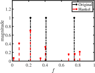
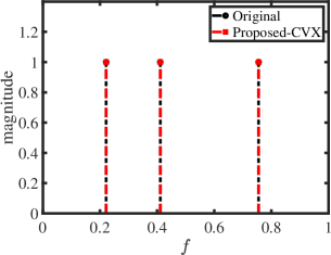
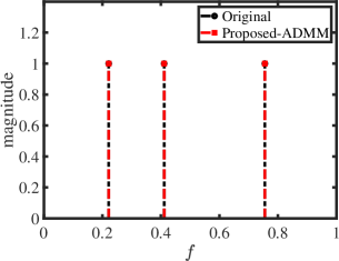
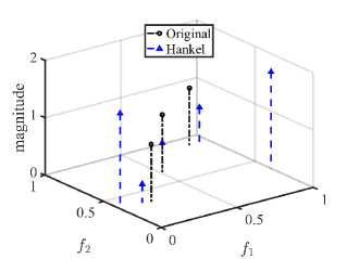
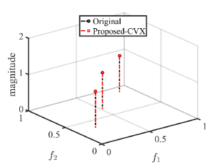
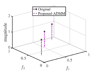
We first show the reconstruction results for standard Hankel matrix completion, the proposed method with CVX solver and the proposed method with ADMM solver. We set n=32n=32, r=3r=3, m=10m=10 and σ=0.5\sigma=0.5. The matrix pencil method is used to estimate the location and amplitude of frequencies [42]. The frequency estimation results are shown in Fig. 1. As expected, with the reliable reference signal, the proposed scheme with different solvers exactly reconstructs the original signal,which has a better performance than standard Hankel matrix completion.

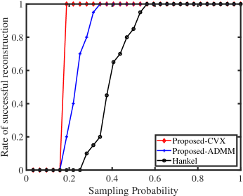
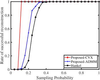
We next provide the successful reconstruction rate as a function of sampling probability standard Hankel matrix completion, the proposed method with CVX solver and the proposed method with ADMM solver. We set n=32n=32, r=3r=3, σ=0.1\sigma=0.1. We set η=104\eta=10^{-4} for CVX solver and η=102\eta=10^{-2} for ADMM solver since CVX solver gets the exact solution while ADMM solver has performance degradation due to finite iteration. For each sampling probability, we sample the desired signals in time domain randomly and the results are averaged over 300 independent trials. Then we count the number of successful trials, and calculate the related probability. Here, we claim a trial as a successful trial if the solution 𝒙\bm{x}^{\dagger} satisfies

𝒙𝒙2𝒙2<η.\frac{\left\lVert\bm{x}^{\star}-\bm{x}^{\dagger}\right\rVert_{2}}{\left\lVert\bm{x}^{\star}\right\rVert_{2}}<\eta.

The results are presented in Fig. 2. The results indicate that the proposed approach (3) outperforms the standard Hankel matrix completion with reliable reference.

TABLE I: Running time comparison for 1-D signals
Methods 1616 6464 9696
Proposed-CVX 0.483s 3.185s 21.456s
Proposed-ADMM 0.003s 0.017s 0.028s

We then compare the running time for the proposed method with different solvers when the dimension of signals is 16,64 and 96. The numerical simulations are carried on an Intel desktop with 2.5 GHz CPU and 8 GB RAM. The results in Table I show that ADMM solver can dramatically improve the running time. Besides, the proposed scheme with ADMM solver has a much better performance compared with the standard Hankel matrix completion.

VI-B Simulations for 2-D signals

We proceed by giving the numerical results for two-dimensional signals.

Consider a two-dimensional spectrally sparse signal 𝑿N1×N2\bm{X}^{\star}\in\mathbb{R}^{N_{1}\times N_{2}} and the signal is a weighted superposition of rr complex sinusoids with unit amplitudes. The reference signal is created by 𝚽=𝑿+σ𝑵\bm{\Phi}=\bm{X}^{\star}+\sigma\bm{N}, where the entries of the real and imaginary part of 𝑵\bm{N} follow i.i.d. standard Gaussian distribution, i.e., Re(Nij),Im(Nij)𝒩(0,1)\mbox{Re}(N_{ij}),\mbox{Im}(N_{ij})\sim\mathcal{N}(0,1) for i=1,,N1,j=1,,N2i=1,\ldots,N_{1},j=1,\ldots,N_{2}.

We first show the recovery results for the proposed method and standard Hankel matrix completion. We set N1=10,N2=10,r=3,m=20N_{1}=10,N_{2}=10,r=3,m=20 and σ=0.1\sigma=0.1. 2D-MUSIC is applied to obtain the location and amplitude of frequencies[43]. The results are presented in Fig. 3. The results show that the proposed method with different solvers can exactly recover the desired signals while Hankel matrix cannot.

We next present the successful reconstruction rate as a function of sampling probability standard Hankel matrix completion, the proposed method with CVX solver and the proposed method with ADMM solver. We set N1=10,N2=10,r=3N_{1}=10,N_{2}=10,r=3 and σ=0.1\sigma=0.1. We increase the number of samples mm from 1 to 100. We Fig. 4 gives the simulation results. As expected, the proposed scheme with the CVX solver performs the best, followed by the proposed scheme with ADMM solver and standard Hankel matrix completion.

TABLE II: Running time comparison for 2-D signals
Methods 8×88\times 8 10×1010\times 10 12×1212\times 12
Proposed-CVX 1.420s 3.449s 12.847s
Proposed-ADMM 0.399s 0.529s 0.786s

Finally, Table II compares the running time for the proposed method with different solvers when N1=N2=8N_{1}=N_{2}=8, N1=N2=10N_{1}=N_{2}=10 and N1=N2=12N_{1}=N_{2}=12. The results present that the proposed scheme with ADMM solver has smaller running time than that with CVX solver, especially when the dimension of signals is large.

VII Conclusion

In this paper, we have integrated prior information to improve the performance of spectrally sparse signal recovery via structured matrix completion problem and have provided the related performance guarantees. Furthermore, we have designed corresponding ADMM algorithm to reduce the computational complexity. Both the theoretical and experimental results show that the proposed scheme outperforms standard Hankel matrix completion.

Appendix A Proof of Theorem 1

Dual certification is used to deviate the theoretical results. In particular, we use the golfing method from [33] to proceed the process. And we adjust the methods from [6, 7] to suit our model.

Recall the definition of the operator 𝒜k:n1×n2n1×n2\mathcal{A}_{k}:\mathbb{C}^{n_{1}\times n_{2}}\to\mathbb{C}^{n_{1}\times n_{2}} by

𝒜k(𝑿)=𝑿,𝑨k𝑨k,k=1,,n.\mathcal{A}_{k}(\bm{X})=\left\langle\bm{X},\bm{A}_{k}\right\rangle\bm{A}_{k},\,k=1,\ldots,n.

Then each 𝒜k\mathcal{A}_{k} is an orthogonal projection onto the one-dimensional subspace spanned by 𝑨k\bm{A}_{k}. The orthogonal projection onto the subspace spanned by {𝑨k}k=1n\{\bm{A}_{k}\}_{k=1}^{n} is given as 𝒜=k=1n𝒜k\mathcal{A}=\sum_{k=1}^{n}\mathcal{A}_{k}. Let 𝒜\mathcal{A}^{\perp} denote the orthogonal complement of 𝒜\mathcal{A}. The summation of the rank-1 projection operators in {𝒜k}kΩ\{\mathcal{A}_{k}\}_{k\in\Omega} is denoted by 𝒜Ω\mathcal{A}_{\Omega}, i.e., 𝒜ΩkΩ𝒜k\mathcal{A}_{\Omega}\triangleq\sum_{k\in\Omega}\mathcal{A}_{k}. Since Ω\Omega is a multi-set and there may exist repetitions in Ω\Omega, 𝒜Ω\mathcal{A}_{\Omega} may be not a projection operator. The summation of distinct elements in {𝒜k}kΩ\{\mathcal{A}_{k}\}_{k\in\Omega} is denoted by 𝒜Ω\mathcal{A}^{\prime}_{\Omega}, which is a valid orthogonal projection.

Before proving the theorem, let’s review the proposed program

min𝒛(𝒛)2λRe(𝒢(ϕ),(𝒛))\displaystyle\min\limits_{\bm{z}}~{}~{}\left\lVert\mathcal{H}(\bm{z})\right\rVert_{*}-2\lambda\,\text{Re}\left(\left\langle\mathcal{G}(\bm{\phi}),\mathcal{H}(\bm{z})\right\rangle\right)
s.t.𝒫Ω(𝒛)=𝒫Ω(𝒙).\displaystyle~{}\text{s.t.}~{}~{}~{}\mathcal{P}_{\Omega}(\bm{z})=\mathcal{P}_{\Omega}({\bm{x}}).

We begin by presenting two lemmas, which are necessary for the proof.

Lemma 1 ([7, Lemma 19] & [6, Lemma 3]).

Suppose that

j=1n2(i=1n1|[𝑨k]i,j|)2=1,andi=1n1(j=1n2|[𝑨k]i,j|)2=1.\sum_{j=1}^{n_{2}}\left(\sum_{i=1}^{n_{1}}|[\bm{A}_{k}]_{i,j}|\right)^{2}=1,~{}\text{and}~{}\sum_{i=1}^{n_{1}}\left(\sum_{j=1}^{n_{2}}|[\bm{A}_{k}]_{i,j}|\right)^{2}=1.

So we have

max1kn𝑼H𝑨kF2\displaystyle\max_{1\leq k\leq n}\left\lVert\bm{U}^{H}\bm{A}_{k}\right\rVert_{F}^{2} μrn1,\displaystyle\leq\frac{\mu r}{n_{1}}, (17)
max1kn𝑽H𝑨kHF2\displaystyle\max_{1\leq k\leq n}\left\lVert\bm{V}^{H}\bm{A}_{k}^{H}\right\rVert_{F}^{2} μrn2.\displaystyle\leq\frac{\mu r}{n_{2}}.

Then for any small constant 0<ϵ120<\epsilon\leq\frac{1}{2}, one has

𝒫𝒯𝒜𝒫𝒯nm𝒫𝒯𝒜Ω𝒫𝒯ϵ\left\lVert\mathcal{P}_{\mathcal{T}}\mathcal{A}\mathcal{P}_{\mathcal{T}}-\frac{n}{m}\mathcal{P}_{\mathcal{T}}\mathcal{A}_{\Omega}\mathcal{P}_{\mathcal{T}}\right\rVert\leq\epsilon (18)

with probability exceeding 1n41-n^{-4}, provided that m>cμcsrlognm>c\mu c_{\mathrm{s}}r\log n for some universal constant c>0c>0 and csmax{nn1,nn2}c_{\mathrm{s}}\triangleq\max\{\frac{n}{n_{1}},\frac{n}{n_{2}}\}.

Lemma 2.

Consider a multi-set Ω\Omega that contains mm random indices. Suppose that the sampling operator 𝒜Ω\mathcal{A}_{\Omega} obeys

𝒫𝒯𝒜𝒫𝒯nm𝒫𝒯𝒜Ω𝒫𝒯12.\left\|\mathcal{P}_{\mathcal{T}}\mathcal{A}\mathcal{P}_{\mathcal{T}}-\frac{n}{m}\mathcal{P}_{\mathcal{T}}\mathcal{A}_{\Omega}\mathcal{P}_{\mathcal{T}}\right\|\leq\frac{1}{2}. (19)

If there exists a matrix 𝐖\bm{W} satisfying

𝒜Ω(𝑾)=0,\mathcal{A}^{\prime}_{\Omega^{\perp}}\left(\bm{W}\right)=0, (20)
𝒫𝒯(sgn[(𝒙)]𝑾λ𝒢(ϕ))F17n,\left\|\mathcal{P}_{\mathcal{T}}\left(\mbox{sgn}[\mathcal{H}(\bm{x}^{\star})]-\bm{W}-\lambda\mathcal{G}(\bm{\phi})\right)\right\|_{F}\leq\frac{1}{7n}, (21)

and

𝒫𝒯(𝑾+λ𝒢(ϕ))12,\left\|\mathcal{P}_{\mathcal{T}^{\perp}}\left(\bm{W}+\lambda\mathcal{G}(\bm{\phi})\right)\right\|\leq\frac{1}{2}, (22)

then the program (3) can achieve exact recovery, i.e., 𝐱\bm{x} is the unique minimizer.

Proof:

See Appendix B. ∎

As shown in [6], we generate j0j_{0} independent random multi-sets {Ωi}i=1j0\{\Omega_{i}\}_{i=1}^{j_{0}} and each set contains mj0\frac{m}{j_{0}} entries. Note that the distribution of Ω\Omega and i=1j0Ωi\cup_{i=1}^{j_{0}}\Omega_{i} is the same. Then we construct of a dual certificate 𝑾\bm{W} via the golfing scheme:

  1. 1.

    Define 𝑭0𝒫𝒯(sgn[(𝒙)]λ𝒢(ϕ))\bm{F}_{0}\triangleq\mathcal{P}_{\mathcal{T}}\left(\mbox{sgn}[\mathcal{H}(\bm{x})]-\lambda\mathcal{G}(\bm{\phi})\right);

  2. 2.

    For every ii (1ij01\leq i\leq j_{0}), set

    𝑭i𝒫𝒯(𝒜nj0m𝒜Ωi)𝒫𝒯(𝑭i1);\bm{F}_{i}\triangleq\mathcal{P}_{\mathcal{T}}\left(\mathcal{A}-\frac{nj_{0}}{m}\mathcal{A}_{\Omega_{i}}\right)\mathcal{P}_{\mathcal{T}}\left(\bm{F}_{i-1}\right);
  3. 3.

    Define 𝑾i=1j0(nj0m𝒜Ωi+𝒜)(𝑭i1)\bm{W}\triangleq\sum_{i=1}^{j_{0}}\left(\frac{nj_{0}}{m}\mathcal{A}_{\Omega_{i}}+\mathcal{A}^{\perp}\right)\left(\bm{F}_{i-1}\right).

By the construction, it’s easy to see that 𝑾\bm{W} is in the range space of 𝒜Ω𝒜\mathcal{A}_{\Omega}\cup\mathcal{A}^{\perp}, then

𝒜Ω(𝑾)=0.\mathcal{A}^{\prime}_{\Omega^{\perp}}\left(\bm{W}\right)=0. (23)

By recursive calculation as [6, Eq. (40)], we can obtain

𝒫𝒯(𝑾𝑭0)=𝒫𝒯(𝑭j0).-\mathcal{P}_{\mathcal{T}}\left(\bm{W}-\bm{F}_{0}\right)=\mathcal{P}_{\mathcal{T}}\left(\bm{F}_{j_{0}}\right). (24)

Using Lemma 1 yields

𝒫𝒯(𝑾𝑭0)F\displaystyle\left\|\mathcal{P}_{\mathcal{T}}\left(\bm{W}-\bm{F}_{0}\right)\right\|_{F} =𝒫𝒯(𝑭j0)F\displaystyle=\left\|\mathcal{P}_{\mathcal{T}}\left(\bm{F}_{j_{0}}\right)\right\|_{F}
𝒫𝒯(𝒜nj0m𝒜Ωi)𝒫𝒯j0𝑭0F\displaystyle\leq\left\lVert\mathcal{P}_{\mathcal{T}}\left(\mathcal{A}-\frac{nj_{0}}{m}\mathcal{A}_{\Omega_{i}}\right)\mathcal{P}_{\mathcal{T}}\right\rVert^{j_{0}}\left\lVert\bm{F}_{0}\right\rVert_{F}
ϵj0𝑭0F12j0𝑭0F.\displaystyle\leq\epsilon^{j_{0}}\left\lVert\bm{F}_{0}\right\rVert_{F}\leq\frac{1}{2^{j_{0}}}\left\lVert\bm{F}_{0}\right\rVert_{F}. (25)

Let

j0=max{log(7n𝑭0F),1},j_{0}=\max\left\{\log\left(7n\left\lVert\bm{F}_{0}\right\rVert_{F}\right),1\right\}, (26)

then we have

𝒫𝒯(𝑾sgn[(𝒙)]+λ𝒢(ϕ))F17n\displaystyle\left\|\mathcal{P}_{\mathcal{T}}\left(\bm{W}-\mbox{sgn}[\mathcal{H}(\bm{x}^{\star})]+\lambda\mathcal{G}(\bm{\phi})\right)\right\|_{F}\leq\frac{1}{7n} (27)

except with a probability at most j0n4=o(n3)j_{0}n^{-4}=o(n^{-3}), as long as

m>cμcsrlognmax{log(7n𝑭0F),1}.m>c\mu c_{\mathrm{s}}r\log n\max\left\{\log\left(7n\left\lVert\bm{F}_{0}\right\rVert_{F}\right),1\right\}.

For the last condition, using triangle’s inequality yields

𝒫𝒯(𝑾+λ𝒢(ϕ))𝒫𝒯(𝑾)+𝒫𝒯(λ𝒢(ϕ)).\left\lVert\mathcal{P}_{\mathcal{T}^{\perp}}\left(\bm{W}+\lambda\mathcal{G}(\bm{\phi})\right)\right\rVert\leq\left\lVert\mathcal{P}_{\mathcal{T}^{\perp}}(\bm{W})\right\rVert+\left\lVert\mathcal{P}_{\mathcal{T}^{\perp}}(\lambda\mathcal{G}(\bm{\phi}))\right\rVert.

According to the result of [6, VI. E], we have

𝒫𝒯(𝑾)\displaystyle\left\lVert\mathcal{P}_{\mathcal{T}^{\perp}}(\bm{W})\right\rVert
l=1j0𝒫𝒯(nj0m𝒜Ωl+𝒜)𝒫𝒯(𝑭l1)\displaystyle\leq\sum_{l=1}^{j_{0}}\left\lVert\mathcal{P}_{\mathcal{T}^{\perp}}\left(\frac{nj_{0}}{m}\mathcal{A}_{\Omega_{l}}+\mathcal{A}^{\perp}\right)\mathcal{P}_{\mathcal{T}}\left(\bm{F}_{l-1}\right)\right\rVert
l=1j0(12)l1(nj0lognm𝑭0𝒜,2+nj0lognm𝑭0𝒜,)\displaystyle\leq\sum_{l=1}^{j_{0}}\small\left(\frac{1}{2}\right)^{l-1}\left(\sqrt{\frac{nj_{0}\log n}{m}}\left\lVert\bm{F}_{0}\right\rVert_{\mathcal{A},2}+\frac{nj_{0}\log n}{m}\left\lVert\bm{F}_{0}\right\rVert_{\mathcal{A},\infty}\right)
<2Δ(𝑭0𝒜,2+𝑭0𝒜,),\displaystyle<\frac{2}{\Delta}(\left\lVert\bm{F}_{0}\right\rVert_{\mathcal{A},2}+\left\lVert\bm{F}_{0}\right\rVert_{\mathcal{A},\infty}),

as long as

mcmax{μcs,ν}max{Δ2,1}rlognmax{log(7n𝑭0F),1},m\geq c\max\{\mu c_{\mathrm{s}},\nu\}\\ \cdot\max\{\Delta^{2},1\}\,r\log n\max\left\{\log\left(7n\left\lVert\bm{F}_{0}\right\rVert_{F}\right),1\right\},

where ν=o(μcslog2n)\nu=o(\mu c_{\mathrm{s}}\log^{2}n) from [7, Appendix E]. Set

Δ=4(𝑭0𝒜,2+𝑭0𝒜,)12𝒫𝒯(λ𝒢(ϕ)).\Delta=\frac{4(\left\lVert\bm{F}_{0}\right\rVert_{\mathcal{A},2}+\left\lVert\bm{F}_{0}\right\rVert_{\mathcal{A},\infty})}{1-2\left\lVert\mathcal{P}_{\mathcal{T}^{\perp}}(\lambda\mathcal{G}(\bm{\phi}))\right\rVert}.

If 𝒫𝒯(λ𝒢(ϕ))<12\left\lVert\mathcal{P}_{\mathcal{T}^{\perp}}(\lambda\mathcal{G}(\bm{\phi}))\right\rVert<\frac{1}{2}, we have

𝒫T(𝑾+λ𝒢(ϕ))12.\left\|\mathcal{P}_{T^{\perp}}\left(\bm{W}+\lambda\mathcal{G}(\bm{\phi})\right)\right\|\leq\frac{1}{2}.

Therefore, we conclude, if

mmax{Δ2,1}cμcsrlog3nmax{log(7n𝑭0F),1},m\geq\max\{\Delta^{2},1\}\,c\mu c_{\mathrm{s}}r\log^{3}n\max\left\{\log\left(7n\left\lVert\bm{F}_{0}\right\rVert_{F}\right),1\right\},

then with high probability, we can achieve the unique minimum.

Remark 5.

Form the operator c(𝒙)\mathcal{H}_{c}(\bm{x}) with wrap-around property, ν=o(μcs)\nu=o(\mu c_{\mathrm{s}}) according to [7, Appendix E]. Therefore, we can get the following bound of sample size

mmax{Δ2,1}cμcsrlognmax{log(7n𝑭0F),1}.m\geq\max\{\Delta^{2},1\}\,c\mu c_{\mathrm{s}}r\log n\max\left\{\log\left(7n\left\lVert\bm{F}_{0}\right\rVert_{F}\right),1\right\}.

Appendix B Proof of Lemma 2

Let 𝒛=𝒙+𝒉\bm{z}=\bm{x}+\bm{h} be the minimizer to (3). We will show that (𝒉)=0\mathcal{H}(\bm{h})=0. Then by the injectivity of the operator \mathcal{H}, we achieve 𝒉=0\bm{h}=0, so we have 𝒛=𝒙\bm{z}=\bm{x}.

According to case 2 in the proof of [7, Lemma 20], 𝒫𝒯((𝒉))F3n𝒫𝒯((𝒉))F\left\lVert\mathcal{P}_{\mathcal{T}}(\mathcal{H}(\bm{h}))\right\rVert_{F}\geq 3n\left\lVert\mathcal{P}_{\mathcal{T}^{\perp}}(\mathcal{H}(\bm{h}))\right\rVert_{F} leads to (𝒉)=0\mathcal{H}(\bm{h})=0. So we only need to prove that when

𝒫𝒯((𝒉))F3n𝒫𝒯((𝒉))F,\left\lVert\mathcal{P}_{\mathcal{T}}(\mathcal{H}(\bm{h}))\right\rVert_{F}\leq 3n\left\lVert\mathcal{P}_{\mathcal{T}^{\perp}}(\mathcal{H}(\bm{h}))\right\rVert_{F}, (28)

we also have (𝒉)=0\mathcal{H}(\bm{h})=0. In the subsequent analysis, we assume that the condition (28) is correct.

According to the definition of nuclear norm, there exists 𝑩\bm{B} such that 𝑩,𝒫𝒯((𝒉))=𝒫𝒯((𝒉))\left\langle\bm{B},\mathcal{P}_{\mathcal{T}^{\perp}}(\mathcal{H}(\bm{h}))\right\rangle=\left\lVert\mathcal{P}_{\mathcal{T}^{\perp}}(\mathcal{H}(\bm{h}))\right\rVert_{*} and 𝑩1\left\lVert\bm{B}\right\rVert\leq 1. Then sgn((𝒙))+𝒫𝒯(𝑩)\mbox{sgn}(\mathcal{H}(\bm{x}))+\mathcal{P}_{\mathcal{T}^{\perp}}(\bm{B}) is a sub-gradient of the nuclear norm at (𝒙)\mathcal{H}(\bm{x}). Then it follows that

(𝒙)+(𝒉)2λRe(𝒢(ϕ),(𝒙)+(𝒉))\displaystyle\left\lVert\mathcal{H}(\bm{x})+\mathcal{H}(\bm{h})\right\rVert_{*}-2\lambda\,\text{Re}\left(\left\langle\mathcal{G}(\bm{\phi}),\mathcal{H}(\bm{x})+\mathcal{H}(\bm{h})\right\rangle\right){} (29)
(𝒙)2λRe(𝒢(ϕ),(𝒙))\displaystyle\geq\left\lVert\mathcal{H}(\bm{x})\right\rVert_{*}-2\lambda\,\text{Re}\left(\left\langle\mathcal{G}(\bm{\phi}),\mathcal{H}(\bm{x})\right\rangle\right)
+2Re(sgn[(𝒙)]+𝒫𝒯(𝑩)λ𝒢(ϕ),(𝒉))\displaystyle\quad+2\,\text{Re}\left(\left\langle\mbox{sgn}[\mathcal{H}(\bm{x})]+\mathcal{P}_{\mathcal{T}^{\perp}}(\bm{B})-\lambda\mathcal{G}(\bm{\phi}),\mathcal{H}(\bm{h})\right\rangle\right)
=(𝒙)2λRe(𝒢(ϕ),(𝒙))+2Re(𝑾,(𝒉))\displaystyle=\left\lVert\mathcal{H}(\bm{x})\right\rVert_{*}-2\lambda\,\text{Re}\left(\left\langle\mathcal{G}(\bm{\phi}),\mathcal{H}(\bm{x})\right\rangle\right)+2\,\text{Re}\left(\left\langle\bm{W},\mathcal{H}(\bm{h})\right\rangle\right)
+2Re(sgn[(𝒙)]+𝒫𝒯(𝑩)λ𝒢(ϕ)𝑾,(𝒉)).\displaystyle\quad+2\,\text{Re}\left(\left\langle\mbox{sgn}[\mathcal{H}(\bm{x})]+\mathcal{P}_{\mathcal{T}^{\perp}}(\bm{B})-\lambda\mathcal{G}(\bm{\phi})-\bm{W},\mathcal{H}(\bm{h})\right\rangle\right).

We can get Re(𝑾,(𝒉))=0\text{Re}\left(\left\langle\bm{W},\mathcal{H}(\bm{h})\right\rangle\right)=0 as shown in [7, A.33-A.34]. In addition, we have

𝒫𝒯(𝑩),(𝒉)\displaystyle\langle\mathcal{P}_{\mathcal{T}^{\perp}}(\bm{B}),~{}\mathcal{H}(\bm{h})\rangle{} =𝒫𝒯(𝑩),𝒫𝒯((𝒉))\displaystyle=\langle\mathcal{P}_{\mathcal{T}^{\perp}}(\bm{B}),~{}\mathcal{P}_{\mathcal{T}^{\perp}}(\mathcal{H}(\bm{h}))\rangle
=𝒫𝒯((𝒉)).\displaystyle=\left\lVert\mathcal{P}_{\mathcal{T}^{\perp}}(\mathcal{H}(\bm{h}))\right\rVert_{*}.

Then the inequality (29) becomes

(𝒙)+(𝒉)2λRe(𝒢(ϕ),(𝒙)+(𝒉))\displaystyle\left\lVert\mathcal{H}(\bm{x})+\mathcal{H}(\bm{h})\right\rVert_{*}-2\lambda\,\text{Re}\left(\left\langle\mathcal{G}(\bm{\phi}),\mathcal{H}(\bm{x})+\mathcal{H}(\bm{h})\right\rangle\right)
(𝒙)2λRe(𝒢(ϕ),(𝒙))+2𝒫𝒯((𝒉))\displaystyle\geq\left\lVert\mathcal{H}(\bm{x})\right\rVert_{*}-2\lambda\,\text{Re}\left(\left\langle\mathcal{G}(\bm{\phi}),\mathcal{H}(\bm{x})\right\rangle\right)+2\left\lVert\mathcal{P}_{\mathcal{T}^{\perp}}(\mathcal{H}(\bm{h}))\right\rVert_{*}
2Re(𝑾sgn[(𝒙)]+λ𝒢(ϕ),(𝒉)).\displaystyle\qquad\quad-2\,\text{Re}\left(\langle\bm{W}-\mbox{sgn}[\mathcal{H}(\bm{x})]+\lambda\mathcal{G}(\bm{\phi}),\mathcal{H}(\bm{h})\rangle\right). (30)

Next, we are going to derive

𝒫𝒯((𝒉))Re(𝑾sgn[(𝒙)]+λ𝒢(ϕ),(𝒉))0.\left\lVert\mathcal{P}_{\mathcal{T}^{\perp}}(\mathcal{H}(\bm{h}))\right\rVert_{*}\\ -\text{Re}\left(\left\langle\bm{W}-\mbox{sgn}[\mathcal{H}(\bm{x})]+\lambda\mathcal{G}(\bm{\phi}),\mathcal{H}(\bm{h})\right\rangle\right)\geq 0.

Noting that Re(x)|x|\text{Re}\left(x\right)\leq|x| for xCx\in C, it’s enough to prove

𝒫𝒯((𝒉))|𝑾sgn[(𝒙)]+λ𝒢(ϕ),(𝒉)|0.\left\lVert\mathcal{P}_{\mathcal{T}^{\perp}}(\mathcal{H}(\bm{h}))\right\rVert_{*}-|\left\langle\bm{W}-\mbox{sgn}[\mathcal{H}(\bm{x})]+\lambda\mathcal{G}(\bm{\phi}),\mathcal{H}(\bm{h})\right\rangle|\geq 0.

By using the triangle inequality, we have

𝒫𝒯((𝒉))|𝑾sgn[(𝒙)]+λ𝒢(ϕ),(𝒉)|\displaystyle\left\lVert\mathcal{P}_{\mathcal{T}^{\perp}}(\mathcal{H}(\bm{h}))\right\rVert_{*}-|\left\langle\bm{W}-\mbox{sgn}[\mathcal{H}(\bm{x})]+\lambda\mathcal{G}(\bm{\phi}),\mathcal{H}(\bm{h})\right\rangle|
𝒫𝒯((𝒉))|𝒫𝒯(𝑾+λ𝒢(ϕ)),(𝒉)|\displaystyle\geq\left\lVert\mathcal{P}_{\mathcal{T}^{\perp}}(\mathcal{H}(\bm{h}))\right\rVert_{*}-|\langle\mathcal{P}_{\mathcal{T}^{\perp}}(\bm{W}+\lambda\mathcal{G}(\bm{\phi})),\mathcal{H}(\bm{h})\rangle|
|𝒫𝒯(𝑾sgn[(𝒙)]+λ𝒢(ϕ)),(𝒉)|.\displaystyle\qquad\qquad-|\langle\mathcal{P}_{\mathcal{T}}(\bm{W}-\mbox{sgn}[\mathcal{H}(\bm{x})]+\lambda\mathcal{G}(\bm{\phi})),\mathcal{H}(\bm{h})\rangle|. (31)

Using Holder’s inequality and the properties of 𝑾\bm{W} (Eqs. (21) and (22)) yields

𝒫𝒯((𝒉))|𝑾sgn[(𝒙)]+λ𝒢(ϕ),(𝒉)|\displaystyle\left\lVert\mathcal{P}_{\mathcal{T}^{\perp}}(\mathcal{H}(\bm{h}))\right\rVert_{*}-|\left\langle\bm{W}-\mbox{sgn}[\mathcal{H}(\bm{x})]+\lambda\mathcal{G}(\bm{\phi}),\mathcal{H}(\bm{h})\right\rangle|
𝒫𝒯((𝒉))𝒫𝒯(𝑾+λ𝒢(ϕ))𝒫𝒯((𝒉))\displaystyle\geq\left\lVert\mathcal{P}_{\mathcal{T}^{\perp}}(\mathcal{H}(\bm{h}))\right\rVert_{*}-\left\lVert\mathcal{P}_{\mathcal{T}^{\perp}}(\bm{W}+\lambda\mathcal{G}(\bm{\phi}))\right\rVert\left\lVert\mathcal{P}_{\mathcal{T}^{\perp}}(\mathcal{H}(\bm{h}))\right\rVert_{*}
𝒫𝒯(𝑾sgn[(𝒙)]+λ𝒢(ϕ))F𝒫𝒯((𝒉))F\displaystyle\qquad\quad-\left\lVert\mathcal{P}_{\mathcal{T}}(\bm{W}-\mbox{sgn}[\mathcal{H}(\bm{x})]+\lambda\mathcal{G}(\bm{\phi}))\right\rVert_{F}\left\lVert\mathcal{P}_{\mathcal{T}}(\mathcal{H}(\bm{h}))\right\rVert_{F}
𝒫𝒯((𝒉))12𝒫𝒯((𝒉))17n𝒫𝒯((𝒉))F\displaystyle\geq\left\lVert\mathcal{P}_{\mathcal{T}^{\perp}}(\mathcal{H}(\bm{h}))\right\rVert_{*}-\frac{1}{2}\left\lVert\mathcal{P}_{\mathcal{T}^{\perp}}(\mathcal{H}(\bm{h}))\right\rVert_{*}-\frac{1}{7n}\left\lVert\mathcal{P}_{\mathcal{T}}(\mathcal{H}(\bm{h}))\right\rVert_{F}
12𝒫𝒯((𝒉))17n𝒫𝒯((𝒉))F.\displaystyle\geq\frac{1}{2}\left\lVert\mathcal{P}_{\mathcal{T}^{\perp}}(\mathcal{H}(\bm{h}))\right\rVert_{*}-\frac{1}{7n}\left\lVert\mathcal{P}_{\mathcal{T}}(\mathcal{H}(\bm{h}))\right\rVert_{F}. (32)

By using Eq. (28), we obtain

𝒫𝒯((𝒉))|𝑾sgn[(𝒙)]+λ𝒢(ϕ),(𝒉)|\displaystyle\left\lVert\mathcal{P}_{\mathcal{T}^{\perp}}(\mathcal{H}(\bm{h}))\right\rVert_{*}-|\left\langle\bm{W}-\mbox{sgn}[\mathcal{H}(\bm{x})]+\lambda\mathcal{G}(\bm{\phi}),\mathcal{H}(\bm{h})\right\rangle|
12𝒫𝒯((𝒉))37𝒫𝒯((𝒉))\displaystyle\geq\frac{1}{2}\left\lVert\mathcal{P}_{\mathcal{T}^{\perp}}(\mathcal{H}(\bm{h}))\right\rVert_{*}-\frac{3}{7}\left\lVert\mathcal{P}_{\mathcal{T}^{\perp}}(\mathcal{H}(\bm{h}))\right\rVert_{*}
=114𝒫𝒯((𝒉))0.\displaystyle=\frac{1}{14}\left\lVert\mathcal{P}_{\mathcal{T}^{\perp}}(\mathcal{H}(\bm{h}))\right\rVert_{*}\geq 0. (33)

Therefore, we get

(𝒙)+(𝒉)2λRe(𝒢(ϕ),(𝒙)+(𝒉))\displaystyle\left\lVert\mathcal{H}(\bm{x})+\mathcal{H}(\bm{h})\right\rVert_{*}-2\lambda\,\text{Re}\left(\left\langle\mathcal{G}(\bm{\phi}),\mathcal{H}(\bm{x})+\mathcal{H}(\bm{h})\right\rangle\right)
(𝒙)2λRe(𝒢(ϕ),(𝒙))+114𝒫𝒯((𝒉)).\displaystyle\geq\left\lVert\mathcal{H}(\bm{x})\right\rVert_{*}-2\lambda\,\text{Re}\left(\left\langle\mathcal{G}(\bm{\phi}),\mathcal{H}(\bm{x})\right\rangle\right)+\frac{1}{14}\left\lVert\mathcal{P}_{\mathcal{T}^{\perp}}(\mathcal{H}(\bm{h}))\right\rVert_{*}. (34)

Since 𝒛=𝒙+𝒉\bm{z}=\bm{x}+\bm{h} be the minimizer to (3), we also have

(𝒙)+(𝒉)2λRe(𝒢(ϕ),(𝒙)+(𝒉))\displaystyle\left\lVert\mathcal{H}(\bm{x})+\mathcal{H}(\bm{h})\right\rVert_{*}-2\lambda\,\text{Re}\left(\left\langle\mathcal{G}(\bm{\phi}),\mathcal{H}(\bm{x})+\mathcal{H}(\bm{h})\right\rangle\right)
(𝒙)2λRe(𝒢(ϕ),(𝒙)).\displaystyle\leq\left\lVert\mathcal{H}(\bm{x})\right\rVert_{*}-2\lambda\,\text{Re}\left(\left\langle\mathcal{G}(\bm{\phi}),\mathcal{H}(\bm{x})\right\rangle\right). (35)

Combining Eqs. (B) and (B), we get 𝒫𝒯((𝒉))=0\mathcal{P}_{\mathcal{T}^{\perp}}(\mathcal{H}(\bm{h}))=0. By using (28), we also have 𝒫𝒯((𝒉))=0\mathcal{P}_{\mathcal{T}}(\mathcal{H}(\bm{h}))=0. So we conclude (𝒉)=0\mathcal{H}(\bm{h})=0 and 𝒉=0\bm{h}=0.

References

  • [1] M. Lustig, D. Donoho, and J. M. Pauly, “Sparse MRI: The application of compressed sensing for rapid MR imaging,” Magnetic Resonance in Medicine: An Official Journal of the International Society for Magnetic Resonance in Medicine, vol. 58, no. 6, pp. 1182–1195, 2007.
  • [2] L. C. Potter, E. Ertin, J. T. Parker, and M. Cetin, “Sparsity and compressed sensing in radar imaging,” Proc. IEEE, vol. 98, no. 6, pp. 1006–1020, 2010.
  • [3] J. A. Tropp, J. N. Laska, M. F. Duarte, J. K. Romberg, and R. G. Baraniuk, “Beyond nyquist: Efficient sampling of sparse bandlimited signals,” arXiv preprint arXiv:0902.0026, 2009.
  • [4] J. L. Paredes, G. R. Arce, and Z. Wang, “Ultra-wideband compressed sensing: Channel estimation,” IEEE J. Sel. Topics Signal Process., vol. 1, no. 3, pp. 383–395, 2007.
  • [5] D. J. Brenner and E. J. Hall, “Computed tomography—an increasing source of radiation exposure,” N. Engl. J. Med., vol. 357, no. 22, pp. 2277–2284, 2007.
  • [6] Y. Chen and Y. Chi, “Robust spectral compressed sensing via structured matrix completion,” IEEE Trans. Inf. Theory, vol. 60, no. 10, pp. 6576–6601, Oct 2014.
  • [7] J. C. Ye, J. M. Kim, K. H. Jin, and K. Lee, “Compressive sampling using annihilating filter-based low-rank interpolation,” IEEE Trans. Inf. Theory, vol. 63, no. 2, pp. 777–801, 2017.
  • [8] J. P. Haldar, D. Hernando, S.-K. Song, and Z.-P. Liang, “Anatomically constrained reconstruction from noisy data,” Magnetic Resonance in Medicine: An Official Journal of the International Society for Magnetic Resonance in Medicine, vol. 59, no. 4, pp. 810–818, 2008.
  • [9] X. Peng, H.-Q. Du, F. Lam, S. D. Babacan, and Z.-P. Liang, “Reference-driven MR image reconstruction with sparsity and support constraints,” in Biomedical Imaging: From Nano to Macro, 2011 IEEE International Symposium on.   IEEE, 2011, pp. 89–92.
  • [10] B. Wu, R. P. Millane, R. Watts, and P. J. Bones, “Prior estimate-based compressed sensing in parallel MRI,” Magn. Reson. Med., vol. 65, no. 1, pp. 83–95, 2011.
  • [11] B. Bilgic, V. K. Goyal, and E. Adalsteinsson, “Multi-contrast reconstruction with bayesian compressed sensing,” Magn. Reson. Med., vol. 66, no. 6, pp. 1601–1615, 2011.
  • [12] X. Qu, Y. Hou, F. Lam, D. Guo, J. Zhong, and Z. Chen, “Magnetic resonance image reconstruction from undersampled measurements using a patch-based nonlocal operator,” Med. Image Anal., vol. 18, no. 6, pp. 843–856, 2014.
  • [13] J. Huang, C. Chen, and L. Axel, “Fast multi-contrast MRI reconstruction,” Magn. Reson. Imaging, vol. 32, no. 10, pp. 1344–1352, 2014.
  • [14] M. Selim, E. A. Rashed, and H. Kudo, “Low-dose multiphase abdominal ct reconstruction with phase-induced swap prior,” in Developments in X-Ray Tomography X, vol. 9967.   International Society for Optics and Photonics, 2016, p. 99671P.
  • [15] G.-H. Chen, J. Tang, and S. Leng, “Prior image constrained compressed sensing (piccs): a method to accurately reconstruct dynamic ct images from highly undersampled projection data sets,” Med. Phys., vol. 35, no. 2, pp. 660–663, 2008.
  • [16] M. Selim, E. A. Rashed, M. A. Atiea, and H. Kudo, “Image reconstruction using self-prior information for sparse-view computed tomography,” in 2018 9th Cairo International Biomedical Engineering Conference (CIBEC).   IEEE, 2018, pp. 146–149.
  • [17] Y. Li, X. Wang, Z. Ding, X. Zhang, Y. Xiang, and X. Yang, “Spectrum recovery for clutter removal in penetrating radar imaging,” IEEE Trans. Geosci. Remote Sens., 2019.
  • [18] M. Vella and J. F. Mota, “Single Image Super-Resolution via CNN Architectures and TV-TV Minimization,” arXiv preprint arXiv:1907.05380, 2019.
  • [19] C. Dong, C. C. Loy, K. He, and X. Tang, “Image super-resolution using deep convolutional networks,” IEEE Trans. Pattern Anal. Mach. Intell., vol. 38, no. 2, pp. 295–307, 2015.
  • [20] J. Kim, J. Kwon Lee, and K. Mu Lee, “Accurate image super-resolution using very deep convolutional networks,” in Proceedings of the IEEE conference on computer vision and pattern recognition, 2016, pp. 1646–1654.
  • [21] E. J. Candès, J. Romberg, and T. Tao, “Robust uncertainty principles: Exact signal reconstruction from highly incomplete frequency information,” IEEE Trans. Inf. Theory, vol. 52, no. 2, pp. 489–509, 2006.
  • [22] D. L. Donoho, “Compressed sensing,” IEEE Trans. Inf. Theory, vol. 52, no. 4, pp. 1289–1306, 2006.
  • [23] G. Tang, B. N. Bhaskar, P. Shah, and B. Recht, “Compressed sensing off the grid,” IEEE Trans. Inf. Theory, vol. 59, no. 11, pp. 7465–7490, 2013.
  • [24] G. Tang, B. N. Bhaskar, and B. Recht, “Near minimax line spectral estimation,” IEEE Trans. Inf. Theory, vol. 61, no. 1, pp. 499–512, 2014.
  • [25] L. Weizman, Y. C. Eldar, and D. Ben Bashat, “Reference-based MRI,” Med. Phys., vol. 43, no. 10, pp. 5357–5369, 2016.
  • [26] K. V. Mishra, M. Cho, A. Kruger, and W. Xu, “Spectral super-resolution with prior knowledge,” IEEE Trans. Signal Process., vol. 63, no. 20, pp. 5342–5357, 2015.
  • [27] Y. Li, X. Zhang, Z. Ding, and X. Wang, “Compressive multidimensional harmonic retrieval with prior knowledge,” arXiv preprint arXiv:1904.11404, 2019.
  • [28] X. Zhang, W. Cui, and Y. Liu, “Recovery of structured signals with prior information via maximizing correlation,” IEEE Trans. Signal Process., vol. 66, no. 12, pp. 3296–3310, June 2018.
  • [29] ——, “Matrix completion with prior subspace information via maximizing correlation,” arXiv preprint arXiv:2001.01152, 2020.
  • [30] M. Fazel, “Matrix rank minimization with applications,” Ph.D. dissertation, PhD thesis, Stanford University, 2002.
  • [31] B. Recht, M. Fazel, and P. A. Parrilo, “Guaranteed minimum-rank solutions of linear matrix equations via nuclear norm minimization,” SIAM Rev., vol. 52, no. 3, pp. 471–501, 2010.
  • [32] E. J. Candès and B. Recht, “Exact matrix completion via convex optimization,” Found. Comput. Math., vol. 9, no. 6, p. 717, 2009.
  • [33] D. Gross, “Recovering low-rank matrices from few coefficients in any basis,” IEEE Trans. Inf. Theory, vol. 57, no. 3, pp. 1548–1566, 2011.
  • [34] J.-F. Cai, T. Wang, and K. Wei, “Fast and provable algorithms for spectrally sparse signal reconstruction via low-rank hankel matrix completion,” Appl. Comput. Harmon. Anal., vol. 46, no. 1, pp. 94–121, 2019.
  • [35] E. J. Candes and Y. Plan, “Matrix completion with noise,” Proc. IEEE, vol. 98, no. 6, pp. 925–936, 2010.
  • [36] S. Boyd, N. Parikh, E. Chu, B. Peleato, J. Eckstein et al., “Distributed optimization and statistical learning via the alternating direction method of multipliers,” Foundations and Trends® in Machine learning, vol. 3, no. 1, pp. 1–122, 2011.
  • [37] N. Srebro, “Learning with matrix factorizations,” Ph.D. dissertation, Massachusetts Institute of Technology, 2004.
  • [38] K. H. Jin, D. Lee, and J. C. Ye, “A general framework for compressed sensing and parallel MRI using annihilating filter based low-rank hankel matrix,” IEEE Trans. Comput. Imaging, vol. 2, no. 4, pp. 480–495, Dec 2016.
  • [39] Z. Wen, W. Yin, and Y. Zhang, “Solving a low-rank factorization model for matrix completion by a nonlinear successive over-relaxation algorithm,” Mathematical Programming Computation, vol. 4, no. 4, pp. 333–361, 2012.
  • [40] M. Grant and S. Boyd, “CVX: Matlab software for disciplined convex programming, version 2.1,” http://cvxr.com/cvx, Mar. 2014.
  • [41] ——, “Graph implementations for nonsmooth convex programs,” in Recent Advances in Learning and Control, ser. Lecture Notes in Control and Information Sciences, V. Blondel, S. Boyd, and H. Kimura, Eds.   Springer-Verlag Limited, 2008, pp. 95–110.
  • [42] Y. Hua and T. K. Sarkar, “Matrix pencil method for estimating parameters of exponentially damped/undamped sinusoids in noise,” IEEE Trans. Acoust., Speech, Signal Process., vol. 38, no. 5, pp. 814–824, 1990.
  • [43] C. R. Berger, B. Demissie, J. Heckenbach, P. Willett, and S. Zhou, “Signal processing for passive radar using ofdm waveforms,” IEEE J. Sel. Topics Signal Process., vol. 4, no. 1, pp. 226–238, 2010.