11email: zhangqm@pmo.ac.cn 22institutetext: Shandong Provincial Key Laboratory of Optical Astronomy and Solar-Terrestrial Environment, Institute of Space Sciences, Shandong University, Weihai 264209, PR China
33institutetext: CAS Key Laboratory of Solar Activity, National Astronomical Observatories, Chinese Academy of Sciences, Beijing 100101, PR China
44institutetext: School of Astronomy and Space Science, University of Chinese Academy of Sciences, Beijing 100049, PR China
Spectroscopic observations of a flare-related coronal jet
Abstract
Context. Coronal jets are ubiquitous in active regions (ARs) and coronal holes.
Aims. In this paper, we study a coronal jet related to a C3.4 circular-ribbon flare in active region 12434 on 2015 October 16.
Methods. The flare and jet were observed in ultraviolet (UV) and extreme ultraviolet (EUV) wavelengths by the Atmospheric Imaging Assembly (AIA) on board the Solar Dynamics Observatory (SDO). The line-of-sight (LOS) magnetograms of the photosphere were observed by the Helioseismic and Magnetic Imager (HMI) on board SDO. The whole event was covered by the Interface Region Imaging Spectrograph (IRIS) during its imaging and spectroscopic observations. Soft X-ray (SXR) fluxes of the flare were recorded by the GOES spacecraft. Hard X-ray (HXR) fluxes at 450 keV were obtained from observations of RHESSI and Fermi. Radio dynamic spectra of the flare were recorded by the ground-based stations belonging to the e-Callisto network.
Results. Two minifilaments were located under a 3D fan-spine structure before flare. The flare was generated by the eruption of one filament. The kinetic evolution of the jet was divided into two phases: a slow rise phase at a speed of 131 km s-1 and a fast rise phase at a speed of 363 km s-1 in the plane-of-sky. The slow rise phase may correspond to the impulsive reconnection at the breakout current sheet. The fast rise phase may correspond to magnetic reconnection at the flare current sheet. The transition between the two phases occurred at 09:00:40 UT. The blueshifted Doppler velocities of the jet in the Si iv 1402.80 Å line range from -34 to -120 km s-1. The accelerated high-energy electrons are composed of three groups. Those propagating upward along open field generate type III radio bursts, while those propagating downward produce HXR emissions and drive chromospheric condensation observed in the Si iv line. The electrons trapped in the rising filament generate a microwave burst lasting for 40 s. Bidirectional outflows at the base of jet are manifested by significant line broadenings of the Si iv line. The blueshifted Doppler velocities of outflows range from -13 to -101 km s-1. The redshifted Doppler velocities of outflows range from 17 to 170 km s-1.
Conclusions. Our multiwavelength observations of the flare-related jet are in favor of the breakout jet model and are important for understanding the acceleration and transport of nonthermal electrons.
Key Words.:
Line: profiles – Magnetic reconnection – Sun: flares – Sun: filaments, prominences – Sun: UV radiation1 Introduction
Jet-like activities as a result of magnetic reconnection are ubiquitous in the solar atmosphere. Small-scale jets with lower energy budgets and shorter lifetimes include spicules (De Pontieu et al., 2004; Samanta et al., 2019), chromospheric jets (Shibata et al., 2007; Liu et al., 2009; Tian et al., 2014a), bidirectional plasma jets related to explosive events (Innes et al., 1997; Li et al., 2018a), coronal nanojets (Antolin et al., 2020) and mini-jets (Chen et al., 2020). Large-scale jets with higher energy budgets and longer lifetimes include H surges (Schmieder et al., 1995; Liu & Kurokawa, 2004) and coronal jets (Cirtain et al., 2007; Savcheva et al., 2007; Shimojo et al., 2007; Raouafi et al., 2016; Shen, 2021). Coronal jets are transient collimated outflows propagating along open magnetic field or large-scale closed loops (Shibata et al., 1992, 1994; Zhang et al., 2012; Huang et al., 2012, 2020). The speeds of jets can reach hundreds of km s-1 (Shimojo et al., 1996; Culhane et al., 2007; Lu et al., 2019). The presence of open field facilitates the escape of electron beams accelerated by reconnection at the jet base and the generation of type III radio bursts (e.g., Krucker et al., 2011; Glesener et al., 2012; Glesener & Fleishman, 2018).
Although the morphology of jets varies from case to case, most of them show an inverse-Y shape or a two-sided shape (Moore et al., 2010; Shen et al., 2019). The temperature of a jet decreases from 10 MK at the base (Shimojo & Shibata, 2000; Chifor et al., 2008; Bain & Fletcher, 2009) to a few MK along the spire (Zhang & Ji, 2014b). Sometimes, the hot, fast extreme ultraviolet (EUV) jet is adjacent to or mixed with the cool, slow H jet (Shen et al., 2017; Sakaue et al., 2017, 2018; Hou et al., 2020). The electron densities of jets range from 108 cm-3 (Young & Muglach, 2014) to 1010 cm-3 (Mulay et al., 2017). Bright and compact blobs (or plasmoids) are discovered in coronal jets (Zhang & Ji, 2014b; Li & Yang, 2019; Zhang & Ni, 2019; Joshi et al., 2020a), which are mainly interpreted by magnetic islands as a result of tearing-mode instability in the current sheet (Wyper et al., 2016; Ni et al., 2017). Recurring jets produced by successive energy release at the same region are common (Chifor et al., 2008; Hong et al., 2019; Lu et al., 2019). Aside from the radial motion, untwisting motions have been detected in helical jets, implying rapid release and transfer of magnetic helicity (Chen et al., 2012; Zhang & Ji, 2014a; Cheung et al., 2015; Doyle et al., 2019; Joshi et al., 2020b).
In spite of substantial investigations on jets using multiwavelength observational data, the triggering mechanism is an important issue that needs to be addressed. Till now, several mechanisms have been proposed, such as magnetic flux emergence and reconnection with pre-existing magnetic fields (Yokoyama & Shibata, 1996; Archontis & Hood, 2013), magnetic cancellation (Panesar et al., 2016; Sterling et al., 2017), minifilament eruption (Sterling et al., 2015; Hong et al., 2017; Li et al., 2018b), and photospheric rotation (Pariat et al., 2009). Wyper et al. (2017) performed three-dimensional (3D) magnetohydrodynamics (MHD) numerical simulations of a coronal jet driven by filament ejection, whereby a region of strongly sheared magnetic field near the solar surface becomes unstable and erupts. The authors concluded that energy is initially released via magnetic reconnection at the thin breakout current sheet above the flux rope, which is followed by continuing energy release at the thin flare current sheet beneath the erupting filament (or flux rope). The kinetic evolution of the jet is apparently divided into a slow rise phase before the flux rope opens up and a fast rise phase after the rope totally opens up, which correspond to magnetic reconnections at the breakout current sheet and flare current sheet, respectively (Wyper et al., 2018, see their Fig. 5). The breakout jet model is verified observationally by the signatures of a rotating jet and fast degradation of the circular flare ribbon following the coherent brightenings of the ribbon associated with the jet (Zhang et al., 2020). Breakout reconnection at the null point of a fan-spine structure is recently evidenced by the bidirectional outflows ejected from the reconnection site (Yang et al., 2020). However, reconnection at the flare current sheet below the jet has not been noticed.
In this paper, we report our multiwavelengths of a coronal jet related to a C3.4 circular-ribbon flare that induced simultaneous transverse oscillations of a coronal loop and a filament (Zhang, 2020). The flare occurred in NOAA active region (AR) 12434 where a series of homologous flares were produced (Zhang et al., 2016a, b). This paper is arranged as follows. Data analysis is described in Sect. 2. The results are presented in Sect. 3 and compared with previous works in Sect. 4. Finally, a brief summary is given in Sect. 5.
2 Observations and data analysis
The C3.4 flare and jet were observed by the Atmospheric Imaging Assembly (AIA; Lemen et al., 2012) on board the Solar Dynamics Observatory (SDO) on 2015 October 16. SDO/AIA takes full-disk images in two ultraviolet (UV; 1600 and 1700 Å) and seven EUV (94, 131, 171, 193, 211, 304, and 335 Å) wavelengths. The line-of-sight (LOS) magnetograms of the photosphere were observed by the Helioseismic and Magnetic Imager (HMI; Scherrer et al., 2012) on board SDO. The level_1 data of AIA and HMI were calibrated using the standard solar software (SSW) program aia_prep.pro and hmi_prep.pro, respectively.
The flare and jet were also observed by the Interface Region Imaging Spectrograph (IRIS; De Pontieu et al., 2014) Slit-Jaw Imager (SJI) in 1330 Å () and 1400 Å () with a field of view (FOV) of 134129. Spectroscopic observation of the flare was in the “large coarse 8-step raster” mode using four spectral windows (C ii, Mg ii, O i, and Si iv). Each raster had 8 steps from east to west and covered an area of 14129. The step cadence and exposure time were 10 s and 8 s. The spectra were preprocessed using the standard SSW programs iris_orbitvar_corr_l2.pro and iris_prep_despike.pro. The Si iv 1402.80 Å line () is optically thin and can be fitted by single or multicomponent Gaussian functions. The reference line center of Si iv is set to be 1402.80 Å (Li et al., 2015a; Yu et al., 2020a). The uncertainty in Doppler velocity is 2 km s-1.
Soft X-ray (SXR) light curves of the flare in 0.54 and 18 Å were recorded by the GOES spacecraft. Hard X-ray (HXR) fluxes of the flare at different energy bands were obtained from observations of the Reuven Ramaty High-Energy Solar Spectroscopic Imager (RHESSI; Lin et al., 2002) and the Gamma-ray Burst Monitor (GBM; Meegan et al., 2009) on board the Fermi spacecraft. The time cadence of Fermi/GBM switched from an ordinary value of 0.256 s before flare to 0.064 s during the flare. Radio dynamic spectra of the flare were recorded by the ground-based stations belonging to the e-Callisto network111http://www.e-callisto.org. The observational parameters are listed in Table 1.
To obtain the 3D magnetic configuration of the AR before flare, we utilize the “weighted optimization” method (Wiegelmann, 2004; Wiegelmann et al., 2012) to perform a nonlinear force-free field (NLFFF) extrapolation based on the photospheric vector magnetograms observed by HMI at 08:48 UT. The azimuthal component of the inverted vector magnetic field was processed to correct the 180 ambiguity (Leka et al., 2009). The vector field in the image plane was transformed to the heliographic plane (Gary & Hagyard, 1990). The extrapolation was carried out within a box of 380400512 uniformly spaced grid points with . The squashing factor (Demoulin et al., 1996; Titov et al., 2002) and twist number (Berger & Prior, 2006) were calculated with the code developed by Liu et al. (2016).
| Instru. | Time | Cad. | Pix. Size | |
|---|---|---|---|---|
| (Å) | (UT) | (s) | (″) | |
| AIA | 94304 | 08:50-09:18 | 12 | 0.6 |
| AIA | 1600 | 08:50-09:18 | 24 | 0.6 |
| HMI | 6173 | 08:48-09:18 | 45 | 0.6 |
| SJI | 1330 | 08:50-09:18 | 9, 10 | 0.166 |
| SJI | 1400 | 08:50-09:18 | 19, 20 | 0.166 |
| GOES | 0.54 | 08:58-09:18 | 2.05 | … |
| GOES | 18 | 08:58-09:18 | 2.05 | … |
| RHESSI | 650 keV | 09:00-09:10 | 4.0 | … |
| GBM | 450 keV | 08:58-09:10 | 0.064 | … |
| KRIM | 250350 MHz | 08:58-09:01 | 0.25 | … |
| blen5m | 0.981.27 GHz | 09:00-09:02 | 0.25 | … |
| ZSTS | 1.411.43 GHz | 09:00-09:02 | 0.25 | … |
3 Results
3.1 Minifilament eruption and circular-ribbon flare
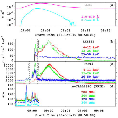
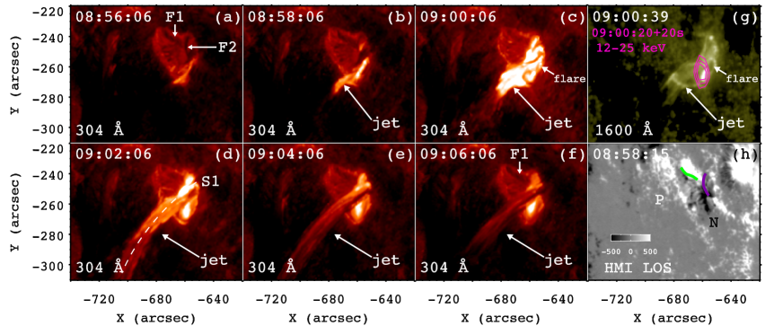
Figure 1(a) shows the SXR light curves of the flare. The SXR emissions started to rise at 08:58 UT and reached peak values at 09:03 UT before declining gradually until 09:12 UT. In Fig. 2, the EUV images observed by AIA in 304 Å illustrate the whole evolution of the event (see also the online movie anim304.mov). Before flare, two short minifilaments (F1 and F2) resided in the AR (panel (a)). With the slow rising of F2, the EUV intensities of the flare started to increase at 08:58 UT and reached peak values at 09:00 UT (panels (b-c)). Meanwhile, a coronal jet propagates in the southeast direction, which was also observed in 1600 Å (panel (g)). The F1 close to F2, however, was undisturbed and survived the flare (panel (f)). Both of the minifilaments were located along the polarity inversion lines (panel (h)). The morphology and evolution of the C3.4 flare were quite analogous to those of C4.2 flare starting at 13:36 UT (Zhang et al., 2016a; Dai et al., 2020).
HXR light curves of the flare recorded by RHESSI and Fermi at different energy bands are plotted in Fig. 1(b-c). Note that there was no observation from RHESSI until 09:00:20 UT. Before 08:59:42 UT, there were two small peaks (panel (c)). The HXR emissions at 1126 keV and 2650 keV started to increase sharply at 08:59:42 UT and peaked at 09:00:20 UT before decreasing to 09:00:40 UT. The HXR peaks indicate that the most drastic release of energy and particle acceleration took place during 08:59:4209:00:40 UT (60 s). Afterwards, the HXR emissions between 4 and 26 keV increased gradually and peaked around 09:02:00 UT before decreasing slowly until 09:04:30 UT, implying their thermal nature from hot plasma (10 MK) as a result of ongoing chromospheric evaporation.
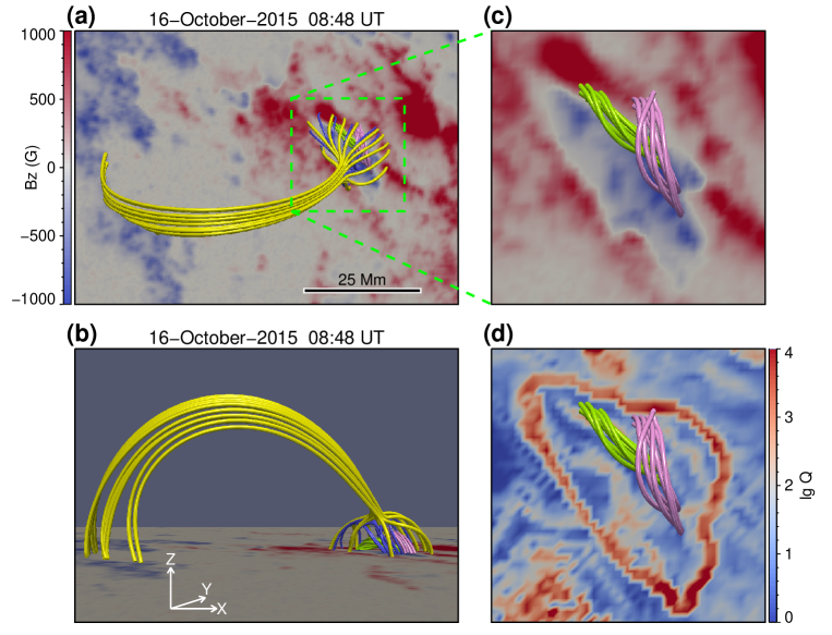
Figure 2(h) shows the LOS magnetogram of the flare region observed by HMI at 08:58:15 UT, featuring a central negative polarity surrounded by positive polarities. Such a magnetic pattern is indicative of the fan-spine topology in the corona (e.g., Zhang et al., 2012; Li et al., 2018b; Hou et al., 2019; Yang et al., 2020). In Fig. 3, the left panels demonstrate the top and side views of 3D magnetic configuration of AR 12434. The fan-spine topology is clearly depicted by the blue and yellow lines, and the outer spine is connected to a remote negative polarity to the southeast of fan dome. Below the dome, the green and light violet lines represent the field lines of F1 and F2, respectively. A close-up of the flare region is displayed in Fig. 2(c). The magnetic fields supporting the two minifilaments are sheared arcades instead of twisted flux ropes. The lies in the range of 0.450.65 for the lower F1 and 0.60.7 for the upper F2. Figure 3(d) shows the spatial distribution of within the flare region, highlighting the closed ribbon of high , which is excellently cospatial with the bright circular ribbon (Fig. 2(c)).
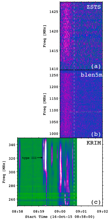
The flare was accompanied by type III radio bursts at 250350 MHz. In Fig. 4, the bottom panel shows the radio dynamic spectra of the flare recorded by e-Callisto/KRIM. The bursts with fast frequency drift rates are noticeable during 08:59:1009:00:40 UT. The radio fluxes at 280, 300, 320, and 340 MHz are extracted and plotted with colored lines in Fig. 1(d). It is revealed that the peaks in radio are roughly correlated with the peaks in HXR, suggesting their common origin. The reconnection-accelerated electrons propagate downward to produce HXR emissions in the chromosphere and propagate upward along open field to produce type III bursts at the same time (Zhang et al., 2016b). Combining with the results of extrapolation in Fig. 3, the real magnetic configuration of the flare region is consistent with previous schematic illustration (Wang & Liu, 2012, see their Fig. 1).
3.2 Coronal jet
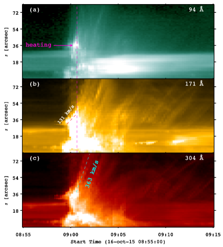
To investigate the radial propagation of the jet, an artificial slice (S1) along the jet spire is selected in Fig. 2(d), which is 80 in length. Time-distance diagrams of S1 in 94 Å (), 171 Å (), and 304 Å () are displayed in Fig. 5. The jet is distinctly observed in all EUV wavelengths, indicating its multithermal nature (Zhang & Ji, 2014b; Joshi et al., 2020a). The kinetic evolution is divided into two phases: a slow rise phase at a plane-of-sky speed of 131 km s-1 and a fast rise phase at a speed of 363 km s-1, respectively. The transition between the two phases occurred at 09:00:40 UT, which is denoted by the magenta dashed line. Impulsive heating to reach a temperature of 6 MK is concurrent with the turning point (panel (a)). The evolution of jet is basically consistent with the breakout model (Wyper et al., 2017, 2018). Magnetic reconnections at the breakout current sheet and flare current sheet lead to intense electron acceleration and heating.
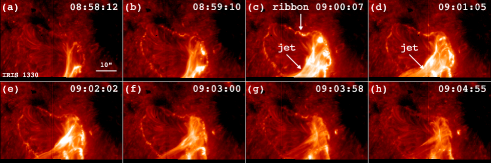
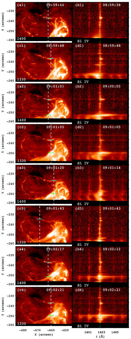
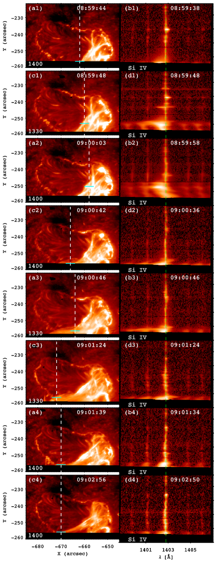
In Fig. 6, the 1330 Å images observed by IRIS/SJI illustrate the evolution of flare and jet in FUV wavelength, which is similar to that in EUV wavelengths. Coherent brightenings of the circular ribbon took place around 09:00:07 UT, indicating null point reconnection (see panel (c) and the online movie anim1330.mov). Unfortunately, the southern part of flare and major part of jet spire were not observed due to the limited FOV of IRIS. The raster observations enable us to carry out spectral analysis of the flare and jet base. In Fig. 7, the left column shows selected FUV images observed by SJI when the jet was covered by the slit. The right column shows the corresponding Si iv spectra of the slit. The spectra of the jet are generally blueshifted, meaning that the jet materials are moving toward the observer.
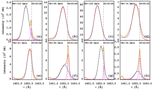
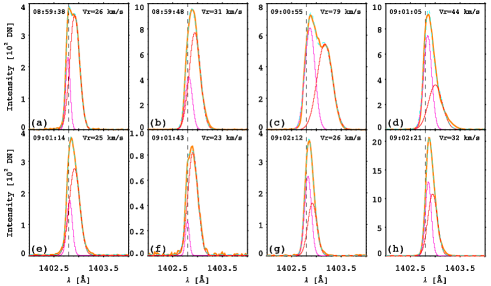
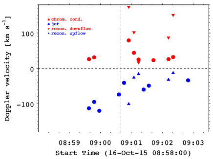
To precisely quantify the Doppler velocities of the jet, the line profiles of Si iv at the positions marked with cyan lines are extracted and plotted with orange lines in Fig. 8. The entirely blueshifted profiles are satisfactorily fitted with a single-Gaussian function (blue lines in panels (b-e)), and the calculated Doppler velocities () are labeled on top of each panel. The profiles with an enhanced blue wing are fitted with a double-Gaussian function (blue and magenta lines in the remaining panels). The sum of two components are drawn with cyan dashed lines, which nicely agree with the observed profiles (orange lines), meaning that the results of double-Gaussian fitting are acceptable. The calculated Doppler velocities () of the blueshifted component are also labeled on top of each panel. In Fig. 12, the values of , ranging from -34 to -120 km s-1, are marked with blue circles.
3.3 Chromospheric condensation
Chromospheric condensation at circular flare ribbons has been observed and investigated in the homologous C3.1 and C4.2 flares (Zhang et al., 2016a, b). The redshifted velocities of the downflow reach up to 60 km s-1 using the observations of Si iv line. The condensation is primarily driven by reconnection-accelerated nonthermal electrons (Li et al., 2015b, 2017). In Fig. 9, likewise, the left column shows selected FUV images observed by SJI when the circular ribbon was covered by the slit. The right column shows the corresponding Si iv spectra of the slit. The spectra of ribbon are redshifted, indicating plasma downflow or chromospheric condensation.
To quantify the Doppler velocities of condensation, the line profiles of Si iv at the positions marked with cyan lines are extracted and plotted with orange lines in Fig. 10. The profiles are fitted with a double-Gaussian function (red and magenta lines), and the sum of two components are drawn with cyan dashed lines, which gratifyingly agree with the observed profiles. The calculated Doppler velocities () of the redshifted component are labeled on top of each panel. In Fig. 12, the values of , ranging from 20 to 80 km s-1, are marked with red circles. The cause of condensation will be discussed in Sect. 4.2.
3.4 Bidirectional outflows
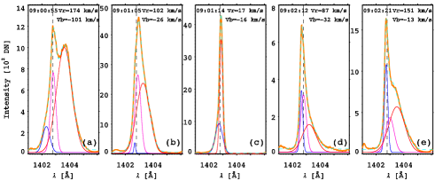
As mentioned before, magnetic reconnection occurs not only at the breakout current sheet above the eruptive filament (or flux rope) but also at the flare current sheet below the flux rope (Wyper et al., 2017, 2018). In Fig. 9, dramatic line broadenings of the Si iv line at the jet base are shown in panels (b2), (b3), (b4), (d2), and (d4), implying simultaneous bidirectional reconnection outflows below the jet (e.g., Tian et al., 2014b; Li et al., 2018c; Xue et al., 2018). To work out the Doppler velocities of outflows, the line profiles of Si iv at the positions marked with short green lines are extracted and plotted with orange lines in Fig. 11. The profiles are fitted with a triple-Gaussian function (blue, magenta, and red lines) except in panel (c), which is fitted with a double-Gaussian function. The sum of multiple components are drawn with cyan dashed lines. The calculated Doppler velocities of the redshifted component () and blueshifted component () are labeled on top of each panel. In Fig. 12, the velocities of reconnection upflow, in the range of -13 and -101 km s-1, are marked with blue triangles. The velocities of reconnection downflow, in the range of 17 to 170 km s-1, are marked with red triangles. We note that the fast reconnection outflows are observed after 09:00:40 UT, when the jet is rising quickly at a speed of 363 km s-1.
It should be emphasized that the chromospheric condensation takes place at the circular ribbon as marked by short cyan lines in Fig. 9. Only redshifted downflow at speeds of 2080 km s-1 could be identified in the spectra (Figs. 9, 10). The bidirectional outflows are observed inside the circular ribbon and close to the jet base. Simultaneous upflow and downflow could be recognized in the spectra (Figs. 9, 11) and the Doppler velocities of bidirectional outflows are significantly higher than those of condensation. These are the main differences between chromospheric condensation and bidirectional outflows.
4 Discussion
4.1 Magnetic reconnection
Magnetic reconnection is believed to play a key role in the energy release of solar flares (Priest & Forbes, 2002; Priest & Pontin, 2009). Direct evidences of reconnection at current sheets are abundant, including the bidirectional inflows and outflows (e.g., Savage et al., 2012; Ning & Guo, 2014; Wu et al., 2016; Xue et al., 2018; Yan et al., 2018; Chen et al., 2020; Yu et al., 2020b), change of magnetic topology (Su et al., 2013), localized heating to 10 MK (Seaton et al., 2017; Li et al., 2018c; Warren et al., 2018), and creation of magnetic islands (Li et al., 2016). Using 3D MHD numerical simulations, Wyper et al. (2017) proposed a universal model for solar eruptions, including eruptive flares and coronal jets. Breakout reconnection around an X-type null point in a quadrupolar magnetic configuration is observed and investigated by Chen et al. (2016). Observations of fast reconnection at the breakout current sheet of a fan-spine structure are carried out by Yang et al. (2020).
In our study, impulsive interchange reconnection at the null point was manifested by coherent brightenings of the circular ribbon, HXR peaks, and type III radio bursts around 09:00:00 UT (Fig. 1(c-d) and Fig. 6(c)). Line broadening as a result of bidirectional outflows was absent before the minifilament broke through the fan surface. During the reconnection at the flare current sheet underneath the filament, pronounced upflows and downflows at the jet base were evidenced by significant Doppler line broadenings of Si iv. The jet did not show untwisting motion during its radial propagation, which is probably due to the small of the sheared arcade supporting the minifilament. Taken as a whole, our multiwavelength observations of the flare-related jet support the breakout jet model (Wyper et al., 2018).
Using combined observations of a small prominence eruption on 2014 May 1, Reeves et al. (2015) found evidence for reconnection between the prominence magnetic field and the overlying field. Reconnection outflows at a plane-of-sky speed of 300 km s-1 and Doppler velocity of 200 km s-1 were detected by SDO/AIA and IRIS, respectively. Moreover, possible reconnection site below the prominence is found (see their Fig. 10). The authors, however, concluded that the reconnection was triggered not by breakout reconnection, but by reconnection occurring along and beneath the prominence.
Using multiwavelength observations from SDO, Hinode/XRT, IRIS, and the DST of Hida Observatory, Sakaue et al. (2018) analyzed a jet-related C5.4 flare on 2014 November 11. The morphology and magnetic configuration of the jet were somewhat similar to the jet in our study. However, the C5.4 flare and jet were caused by magnetic reconnection between the emerging magnetic flux of the satellite spots and the pre-existing ambient fields (Sakaue et al., 2017). Part of the cool H jet experienced secondary acceleration between the trajactories of the H jet and the hot SXR jet after it had been ejected from the lower atmosphere, which is explained by magnetic reconnection between the preceding H jet and the plasmoid in the subsequent SXR jet. In our case, the circular-ribbon flare was caused by eruption of a minifilament underlying the null point (Figs. 2, 3). The fast rise of the jet after 09:00:40 UT may result from quick ejection of F2 after null-point reconnection (Wyper et al., 2018). The reconnection upflow at the flare current sheet may also contribute to the acceleration of jet, as in the case of coronal mass ejections (CMEs; Zhang et al., 2004).
4.2 Cause of chromospheric condensation
As mentioned above, chromospheric condensation could be driven by electron beam heating (e.g., Li et al., 2015a, b; Yu et al., 2020a). During the C4.2 flare on 2015 October 16, explosive chromospheric evaporation took place, which was characterized by plasma upflow at speeds of 35120 km s-1 in the Fe xxi 1354.09 Å line () and downflow at speeds of 1060 km s-1 in the Si iv 1393.77 Å line (Zhang et al., 2016a). The estimated nonthermal energy flux above 20 keV exceeds the threshold (1010 erg s-1 cm-2) for explosive evaporation (Fisher et al., 1985). Condensation during the C3.1 flare associated with a type III burst is also believed to be driven by electron beams (Zhang et al., 2016b).
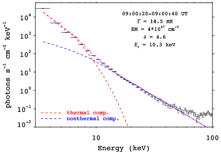
To explore the cause of condensation during the C3.4 flare, we focus on nonthermal electrons as usual. In Fig. 2(g), the AIA 1600 Å image at 09:00:39 UT is superposed with intensity contours of HXR emission at 1225 keV during 09:00:2009:00:40 UT (magenta lines). The centroid of the single HXR source is cospatial with the bright inner ribbon, where majority of nonthermal electrons are precipitated. In Fig. 13, the HXR spectrum obtained from RHESSI observation is fitted with a thermal component plus a thick-target, nonthermal component consisting of a broken power law (Rubio da Costa et al., 2015):
| (1) |
where and represent the spectral index and cutoff energy of nonthermal electrons. denotes the total electron flux above . The fitted thermal component is plotted with a red dashed line, with the values of thermal temperature (), emission measure (EM) being labeled. The fitted nonthermal component is plotted with a blue dashed line, with the values of and being labeled as well. The sum of two components (magenta dashed line) agrees with the observed spectrum.
Before 09:00:40 UT, the HXR emissions were predominantly produced by nonthermal electrons (Fig. 1(c)). The power of injected electrons above is expressed as:
| (2) |
Substituting the parameters obtained from HXR spectral fitting in Fig. 13: , electrons s-1, keV, then is estimated to be 1.31028 erg s-1. A lower limit of the total nonthermal energy in electrons is 2.61029 erg, since there was no RHESSI observation before 09:00:20 UT. Considering that the area of HXR source is in the range of (0.251)1018 cm2, the total nonthermal energy flux is estimated to be (1.35.2)1010 erg s-1 cm-2, which is adequate to drive chromospheric condensation at flare ribbon.
After 09:00:40 UT, the HXR emission at 2550 keV decreased to the pre-eruption level, while the emission at 1225 keV increased gradually with episodic spikes till 09:02:00 UT. To investigate the role of heat conduction in driving condensation, we estimate the energy flux of heat conduction using the expression:
| (3) |
where erg s-1 cm-1 K-7/2, MK denotes the thermal temperature in the corona, and denotes the length scale of the temperature gradient ( represents the equivalent diameter of circular ribbon). is estimated to be 5.5109 erg s-1 cm-2. Therefore, the condensation after 09:00:40 UT should be driven by a combination of nonthermal electrons and heat conduction (Sadykov et al., 2015).
4.3 Emission mechanism of microwave burst
As mentioned above, the flare was associated with type III radio bursts, which are generated by electron beams propagating upward along open field (Innes et al., 2011; Chen et al., 2018). The top and middle panels of Fig. 4 show radio dynamic spectra recorded by ZSTS and blen5m during 09:0009:02 UT with the same cadence as KRIM. Enhancement of the microwave emission at 0.981.43 GHz was obviously demonstrated before 09:00:40 UT. Contrary to the discrete type III bursts owing to the coherent plasma radiation mechanism (Dulk, 1985), the microwave burst seems to be continuous and has no one-to-one correspondence with the type III bursts, implying that the microwave burst was not produced by plasma radiation mechanism. To interpret the relationship between the HXR and radio time profiles of single-loop flares, Kundu et al. (2001) proposed a simple trap model by introducing a critical pitch angle (i.e. loss cone angle). Those injected high-energy electrons with smaller pitch angles are not reflected by the increasing magnetic field as they approach the loop footpoints and will precipitate on their first approach. The remaining electrons with pitch angles outside the loss cone will be trapped in the loop unless pitch angle scattering takes place.
In our case, the accelerated nonthermal electrons before 09:00:40 UT are composed of three groups. The first group propagates along open field to generate type III radio bursts (Fig. 4(c)). The second group precipitates straightforward into the chromosphere and generates HXR emissions (Fig. 1(b-c)). The third group is trapped in the rising minifilament and generates microwave burst through the gyrosynchrotron emission mechanism (Dulk, 1985; Lee & Gary, 2000; Wu et al., 2016). Of course, the trapped electrons will eventually precipitate once pitch angle scattering switches on. Existence of trapped nonthermal electrons in a kink-unstable filament undergoing a failed eruption has been reported by Guo et al. (2012). After the minifilament breaks through the null point and totally opens up, there are no trapped electrons any more and the microwave emission vanishes. This scenario is qualitative and needs to be validated by in-depth investigations. Additional cases of microwave bursts like in Fig. 4 have been collected, which will be the topic of our next paper.
5 Summary
In this work, a coronal jet related to a C3.4 flare in AR 12434 on 2015 October 16 is studied in detail. The main results are summarized as follows:
-
1.
Two minifilaments were located under a 3D fan-spine structure before flare. The flare was generated by the eruption of one filament. The kinetic evolution of the jet was divided into two phases: a slow rise phase at a speed of 130 km s-1 and a fast rise phase at a speed of 360 km s-1 in the plane-of-sky. The slow rise phase may correspond to breakout reconnection at the breakout current sheet, and the fast rise phase may correspond to reconnection at the flare current sheet. The transition between the two phases took place at 09:00:40 UT. The blueshifted Doppler velocities of the jet in the Si iv 1402.80 Å line range from -34 to -120 km s-1.
-
2.
The accelerated high-energy electrons are composed of three groups. Those propagating upward along open field generate type III radio bursts, while those propagating downward produce HXR emissions and drive chromospheric condensation. The electrons trapped in the rising filament generate a microwave burst lasting for 40 s.
-
3.
Bidirectional outflows at the jet base are manifested by significant line broadenings of the Si iv line. The blueshifted Doppler velocities range from -13 to -101 km s-1. The redshifted Doppler velocities range from 17 to 170 km s-1. Our multiwavelength observations of the flare-related jet are in favor of the breakout jet model and shed light on the acceleration and transport of nonthermal electrons.
Acknowledgements.
The authors thank the referee for constructive suggestions and comments. The authors appreciate Drs. Xiaoli Yan in Yunnan Observatories, Ying Li and Lei Lu in Purple Mountain Observatory, Yang Guo in Nanjing University, and Sijie Yu in New Jersey Institute of Technology for valuable discussions. SDO is a mission of NASA’s Living With a Star Program. AIA and HMI data are courtesy of the NASA/SDO science teams. This work is funded by NSFC grants (No. 11773079, 11790302, U1831112, 11903050, 11790304, 11973092, 11573072, and 11703017), the International Cooperation and Interchange Program (11961131002), the Youth Innovation Promotion Association CAS, CAS Key Laboratory of Solar Activity, National Astronomical Observatories (KLSA202003, KLSA202006), and the project supported by the Specialized Research Fund for State Key Laboratories.References
- Antolin et al. (2020) Antolin, P., Pagano, P., Testa, P., et al. 2020, Nature Astronomy. doi:10.1038/s41550-020-1199-8
- Archontis & Hood (2013) Archontis, V., & Hood, A. W. 2013, ApJ, 769, L21. doi:10.1088/2041-8205/769/2/L21
- Bain & Fletcher (2009) Bain, H. M., & Fletcher, L. 2009, A&A, 508, 1443. doi:10.1051/0004-6361/200911876
- Berger & Prior (2006) Berger, M. A., & Prior, C. 2006, Journal of Physics A Mathematical General, 39, 8321. doi:10.1088/0305-4470/39/26/005
- Chen et al. (2012) Chen, H.-D., Zhang, J., & Ma, S.-L. 2012, Research in Astronomy and Astrophysics, 12, 573. doi:10.1088/1674-4527/12/5/009
- Chen et al. (2016) Chen, Y., Du, G., Zhao, D., et al. 2016, ApJ, 820, L37. doi:10.3847/2041-8205/820/2/L37
- Chen et al. (2018) Chen, B., Yu, S., Battaglia, M., et al. 2018, ApJ, 866, 62. doi:10.3847/1538-4357/aadb89
- Chen et al. (2020) Chen, B., Shen, C., Gary, D. E., et al. 2020, Nature Astronomy, doi:10.1038/s41550-020-1147-7
- Chen et al. (2020) Chen, H., Zhang, J., De Pontieu, B., et al. 2020, ApJ, 899, 19. doi:10.3847/1538-4357/ab9cad
- Cheung et al. (2015) Cheung, M. C. M., De Pontieu, B., Tarbell, T. D., et al. 2015, ApJ, 801, 83. doi:10.1088/0004-637X/801/2/83
- Chifor et al. (2008) Chifor, C., Isobe, H., Mason, H. E., et al. 2008, A&A, 491, 279. doi:10.1051/0004-6361:200810265
- Cirtain et al. (2007) Cirtain, J. W., Golub, L., Lundquist, L., et al. 2007, Science, 318, 1580. doi:10.1126/science.1147050
- Culhane et al. (2007) Culhane, L., Harra, L. K., Baker, D., et al. 2007, PASJ, 59, S751. doi:10.1093/pasj/59.sp3.S751
- Dai et al. (2020) Dai, J., Zhang, Q. M., Su, Y. N., et al. 2020, arXiv:2012.07074
- Demoulin et al. (1996) Demoulin, P., Henoux, J. C., Priest, E. R., et al. 1996, A&A, 308, 643
- De Pontieu et al. (2004) De Pontieu, B., Erdélyi, R., & James, S. P. 2004, Nature, 430, 536. doi:10.1038/nature02749
- De Pontieu et al. (2014) De Pontieu, B., Title, A. M., Lemen, J. R., et al. 2014, Sol. Phys., 289, 2733. doi:10.1007/s11207-014-0485-y
- Doyle et al. (2019) Doyle, L., Wyper, P. F., Scullion, E., et al. 2019, ApJ, 887, 246. doi:10.3847/1538-4357/ab5d39
- Dulk (1985) Dulk, G. A. 1985, ARA&A, 23, 169. doi:10.1146/annurev.aa.23.090185.001125
- Fisher et al. (1985) Fisher, G. H., Canfield, R. C., & McClymont, A. N. 1985, ApJ, 289, 425. doi:10.1086/162902
- Gary & Hagyard (1990) Gary, G. A., & Hagyard, M. J. 1990, Sol. Phys., 126, 21. doi:10.1007/BF00158295
- Glesener et al. (2012) Glesener, L., Krucker, S., & Lin, R. P. 2012, ApJ, 754, 9. doi:10.1088/0004-637X/754/1/9
- Glesener & Fleishman (2018) Glesener, L., & Fleishman, G. D. 2018, ApJ, 867, 84. doi:10.3847/1538-4357/aacefe
- Guo et al. (2012) Guo, Y., Ding, M. D., Schmieder, B., et al. 2012, ApJ, 746, 17. doi:10.1088/0004-637X/746/1/17
- Hong et al. (2017) Hong, J., Jiang, Y., Yang, J., et al. 2017, ApJ, 835, 35. doi:10.3847/1538-4357/835/1/35
- Hong et al. (2019) Hong, J., Yang, J., Chen, H., et al. 2019, ApJ, 874, 146. doi:10.3847/1538-4357/ab0c9d
- Hou et al. (2019) Hou, Y., Li, T., Yang, S., et al. 2019, ApJ, 871, 4. doi:10.3847/1538-4357/aaf4f4
- Hou et al. (2020) Hou, Y. J., Li, T., Zhong, S. H., et al. 2020, A&A, 642, A44. doi:10.1051/0004-6361/202038668
- Huang et al. (2012) Huang, Z., Madjarska, M. S., Doyle, J. G., et al. 2012, A&A, 548, A62. doi:10.1051/0004-6361/201220079
- Huang et al. (2020) Huang, Z., Zhang, Q., Xia, L., et al. 2020, ApJ, 897, 113. doi:10.3847/1538-4357/ab96bd
- Innes et al. (1997) Innes, D. E., Inhester, B., Axford, W. I., et al. 1997, Nature, 386, 811. doi:10.1038/386811a0
- Innes et al. (2011) Innes, D. E., Cameron, R. H., & Solanki, S. K. 2011, A&A, 531, L13. doi:10.1051/0004-6361/201117255
- Joshi et al. (2020a) Joshi, R., Chandra, R., Schmieder, B., et al. 2020a, A&A, 639, A22. doi:10.1051/0004-6361/202037806
- Joshi et al. (2020b) Joshi, R., Schmieder, B., Aulanier, G., et al. 2020b, A&A, 642, A169. doi:10.1051/0004-6361/202038562
- Krucker et al. (2011) Krucker, S., Kontar, E. P., Christe, S., et al. 2011, ApJ, 742, 82. doi:10.1088/0004-637X/742/2/82
- Kundu et al. (2001) Kundu, M. R., White, S. M., Shibasaki, K., et al. 2001, ApJ, 547, 1090. doi:10.1086/318422
- Lee & Gary (2000) Lee, J., & Gary, D. E. 2000, ApJ, 543, 457. doi:10.1086/317080
- Leka et al. (2009) Leka, K. D., Barnes, G., Crouch, A. D., et al. 2009, Sol. Phys., 260, 83. doi:10.1007/s11207-009-9440-8
- Lemen et al. (2012) Lemen, J. R., Title, A. M., Akin, D. J., et al. 2012, Sol. Phys., 275, 17. doi:10.1007/s11207-011-9776-8
- Li et al. (2015a) Li, Y., Ding, M. D., Qiu, J., et al. 2015, ApJ, 811, 7. doi:10.1088/0004-637X/811/1/7
- Li et al. (2015b) Li, D., Ning, Z. J., & Zhang, Q. M. 2015, ApJ, 813, 59. doi:10.1088/0004-637X/813/1/59
- Li et al. (2016) Li, L., Zhang, J., Peter, H., et al. 2016, Nature Physics, 12, 847. doi:10.1038/nphys3768
- Li et al. (2017) Li, D., Ning, Z. J., Huang, Y., et al. 2017, ApJ, 841, L9. doi:10.3847/2041-8213/aa71b0
- Li et al. (2018a) Li, D., Li, L., & Ning, Z. 2018, MNRAS, 479, 2382. doi:10.1093/mnras/sty1712
- Li et al. (2018b) Li, T., Yang, S., Zhang, Q., et al. 2018, ApJ, 859, 122. doi:10.3847/1538-4357/aabe84
- Li et al. (2018c) Li, Y., Xue, J. C., Ding, M. D., et al. 2018, ApJ, 853, L15. doi:10.3847/2041-8213/aaa6c0
- Li & Yang (2019) Li, H., & Yang, J. 2019, ApJ, 872, 87. doi:10.3847/1538-4357/aafb3a
- Lin et al. (2002) Lin, R. P., Dennis, B. R., Hurford, G. J., et al. 2002, Sol. Phys., 210, 3. doi:10.1023/A:1022428818870
- Liu & Kurokawa (2004) Liu, Y. & Kurokawa, H. 2004, ApJ, 610, 1136. doi:10.1086/421715
- Liu et al. (2009) Liu, W., Berger, T. E., Title, A. M., et al. 2009, ApJ, 707, L37. doi:10.1088/0004-637X/707/1/L37
- Liu et al. (2016) Liu, R., Kliem, B., Titov, V. S., et al. 2016, ApJ, 818, 148. doi:10.3847/0004-637X/818/2/148
- Lu et al. (2019) Lu, L., Feng, L., Li, Y., et al. 2019, ApJ, 887, 154. doi:10.3847/1538-4357/ab530c
- Meegan et al. (2009) Meegan, C., Lichti, G., Bhat, P. N., et al. 2009, ApJ, 702, 791. doi:10.1088/0004-637X/702/1/791
- Moore et al. (2010) Moore, R. L., Cirtain, J. W., Sterling, A. C., & Falconer, D. A. 2010, ApJ, 720, 757. doi:10.1088/0004-637X/720/1/757
- Mulay et al. (2017) Mulay, S. M., Del Zanna, G., & Mason, H. 2017, A&A, 606, A4. doi:10.1051/0004-6361/201730429
- Ni et al. (2017) Ni, L., Zhang, Q.-M., Murphy, N. A., et al. 2017, ApJ, 841, 27. doi:10.3847/1538-4357/aa6ffe
- Ning & Guo (2014) Ning, Z., & Guo, Y. 2014, ApJ, 794, 79. doi:10.1088/0004-637X/794/1/79
- Panesar et al. (2016) Panesar, N. K., Sterling, A. C., Moore, R. L., et al. 2016, ApJ, 832, L7. doi:10.3847/2041-8205/832/1/L7
- Pariat et al. (2009) Pariat, E., Antiochos, S. K., & DeVore, C. R. 2009, ApJ, 691, 61. doi:10.1088/0004-637X/691/1/61
- Priest & Forbes (2002) Priest, E. R., & Forbes, T. G. 2002, A&A Rev., 10, 313. doi:10.1007/s001590100013
- Priest & Pontin (2009) Priest, E. R., & Pontin, D. I. 2009, Physics of Plasmas, 16, 122101. doi:10.1063/1.3257901
- Raouafi et al. (2016) Raouafi, N. E., Patsourakos, S., Pariat, E., et al. 2016, Space Sci. Rev., 201, 1. doi:10.1007/s11214-016-0260-5
- Reeves et al. (2015) Reeves, K. K., McCauley, P. I., & Tian, H. 2015, ApJ, 807, 7. doi:10.1088/0004-637X/807/1/7
- Rubio da Costa et al. (2015) Rubio da Costa, F., Kleint, L., Petrosian, V., et al. 2015, ApJ, 804, 56. doi:10.1088/0004-637X/804/1/56
- Sadykov et al. (2015) Sadykov, V. M., Vargas Dominguez, S., Kosovichev, A. G., et al. 2015, ApJ, 805, 167. doi:10.1088/0004-637X/805/2/167
- Sakaue et al. (2017) Sakaue, T., Tei, A., Asai, A., et al. 2017, PASJ, 69, 80. doi:10.1093/pasj/psx071
- Sakaue et al. (2018) Sakaue, T., Tei, A., Asai, A., et al. 2018, PASJ, 70, 99. doi:10.1093/pasj/psx133
- Samanta et al. (2019) Samanta, T., Tian, H., Yurchyshyn, V., et al. 2019, Science, 366, 890. doi:10.1126/science.aaw2796
- Savage et al. (2012) Savage, S. L., Holman, G., Reeves, K. K., et al. 2012, ApJ, 754, 13. doi:10.1088/0004-637X/754/1/13
- Savcheva et al. (2007) Savcheva, A., Cirtain, J., Deluca, E. E., et al. 2007, PASJ, 59, S771. doi:10.1093/pasj/59.sp3.S771
- Scherrer et al. (2012) Scherrer, P. H., Schou, J., Bush, R. I., et al. 2012, Sol. Phys., 275, 207. doi:10.1007/s11207-011-9834-2
- Schmieder et al. (1995) Schmieder, B., Shibata, K., van Driel-Gesztelyi, L., et al. 1995, Sol. Phys., 156, 245. doi:10.1007/BF00670226
- Seaton et al. (2017) Seaton, D. B., Bartz, A. E., & Darnel, J. M. 2017, ApJ, 835, 139. doi:10.3847/1538-4357/835/2/139
- Shen et al. (2017) Shen, Y., Liu, Y. D., Su, J., et al. 2017, ApJ, 851, 67. doi:10.3847/1538-4357/aa9a48
- Shen et al. (2019) Shen, Y., Qu, Z., Yuan, D., et al. 2019, ApJ, 883, 104. doi:10.3847/1538-4357/ab3a4d
- Shen (2021) Shen, Y. 2021, arXiv:2101.04846
- Shibata et al. (1992) Shibata, K., Ishido, Y., Acton, L. W., et al. 1992, PASJ, 44, L173
- Shibata et al. (1994) Shibata, K., Nitta, N., Strong, K. T., et al. 1994, ApJ, 431, L51. doi:10.1086/187470
- Shibata et al. (2007) Shibata, K., Nakamura, T., Matsumoto, T., et al. 2007, Science, 318, 1591. doi:10.1126/science.1146708
- Shimojo et al. (1996) Shimojo, M., Hashimoto, S., Shibata, K., et al. 1996, PASJ, 48, 123. doi:10.1093/pasj/48.1.123
- Shimojo & Shibata (2000) Shimojo, M., & Shibata, K. 2000, ApJ, 542, 1100. doi:10.1086/317024
- Shimojo et al. (2007) Shimojo, M., Narukage, N., Kano, R., et al. 2007, PASJ, 59, S745. doi:10.1093/pasj/59.sp3.S745
- Sterling et al. (2015) Sterling, A. C., Moore, R. L., Falconer, D. A., & Adams, M. 2015, Nature, 523, 437. doi:10.1038/nature14556
- Sterling et al. (2017) Sterling, A. C., Moore, R. L., Falconer, D. A., et al. 2017, ApJ, 844, 28. doi:10.3847/1538-4357/aa7945
- Su et al. (2013) Su, Y., Veronig, A. M., Holman, G. D., et al. 2013, Nature Physics, 9, 489. doi:10.1038/nphys2675
- Tian et al. (2014a) Tian, H., DeLuca, E. E., Cranmer, S. R., et al. 2014, Science, 346, 1255711. doi:10.1126/science.1255711
- Tian et al. (2014b) Tian, H., Li, G., Reeves, K. K., et al. 2014, ApJ, 797, L14. doi:10.1088/2041-8205/797/2/L14
- Titov et al. (2002) Titov, V. S., Hornig, G., & Démoulin, P. 2002, Journal of Geophysical Research (Space Physics), 107, 1164. doi:10.1029/2001JA000278
- Wang & Liu (2012) Wang, H., & Liu, C. 2012, ApJ, 760, 101. doi:10.1088/0004-637X/760/2/101
- Warren et al. (2018) Warren, H. P., Brooks, D. H., Ugarte-Urra, I., et al. 2018, ApJ, 854, 122. doi:10.3847/1538-4357/aaa9b8
- Wiegelmann (2004) Wiegelmann, T. 2004, Sol. Phys., 219, 87. doi:10.1023/B:SOLA.0000021799.39465.36
- Wiegelmann et al. (2012) Wiegelmann, T., Thalmann, J. K., Inhester, B., et al. 2012, Sol. Phys., 281, 37. doi:10.1007/s11207-012-9966-z
- Wu et al. (2016) Wu, Z., Chen, Y., Huang, G., et al. 2016, ApJ, 820, L29. doi:10.3847/2041-8205/820/2/L29
- Wyper et al. (2016) Wyper, P. F., DeVore, C. R., Karpen, J. T., et al. 2016, ApJ, 827, 4. doi:10.3847/0004-637X/827/1/4
- Wyper et al. (2017) Wyper, P. F., Antiochos, S. K., & DeVore, C. R. 2017, Nature, 544, 452. doi:10.1038/nature22050
- Wyper et al. (2018) Wyper, P. F., DeVore, C. R., & Antiochos, S. K. 2018, ApJ, 852, 98. doi:10.3847/1538-4357/aa9ffc
- Xue et al. (2018) Xue, Z., Yan, X., Yang, L., et al. 2018, ApJ, 858, L4. doi:10.3847/2041-8213/aabe77
- Yan et al. (2018) Yan, X. L., Yang, L. H., Xue, Z. K., et al. 2018, ApJ, 853, L18. doi:10.3847/2041-8213/aaa6c2
- Yang et al. (2020) Yang, S., Zhang, Q., Xu, Z., et al. 2020, ApJ, 898, 101. doi:10.3847/1538-4357/ab9ac7
- Yokoyama & Shibata (1996) Yokoyama, T., & Shibata, K. 1996, PASJ, 48, 353. doi:10.1093/pasj/48.2.353
- Young & Muglach (2014) Young, P. R., & Muglach, K. 2014, Sol. Phys., 289, 3313. doi:10.1007/s11207-014-0484-z
- Yu et al. (2020a) Yu, K., Li, Y., Ding, M. D., et al. 2020a, ApJ, 896, 154. doi:10.3847/1538-4357/ab9014
- Yu et al. (2020b) Yu, S., Chen, B., Reeves, K. K., et al. 2020b, ApJ, 900, 17. doi:10.3847/1538-4357/aba8a6
- Zhang et al. (2004) Zhang, J., Dere, K. P., Howard, R. A., et al. 2004, ApJ, 604, 420. doi:10.1086/381725
- Zhang et al. (2012) Zhang, Q. M., Chen, P. F., Guo, Y., et al. 2012, ApJ, 746, 19. doi:10.1088/0004-637X/746/1/19
- Zhang & Ji (2014a) Zhang, Q. M., & Ji, H. S. 2014a, A&A, 561, A134. doi:10.1051/0004-6361/201322616
- Zhang & Ji (2014b) Zhang, Q. M., & Ji, H. S. 2014b, A&A, 567, A11. doi:10.1051/0004-6361/201423698
- Zhang et al. (2016a) Zhang, Q. M., Li, D., Ning, Z. J., et al. 2016a, ApJ, 827, 27. doi:10.3847/0004-637X/827/1/27
- Zhang et al. (2016b) Zhang, Q. M., Li, D., & Ning, Z. J. 2016b, ApJ, 832, 65. doi:10.3847/0004-637X/832/1/65
- Zhang & Ni (2019) Zhang, Q. M., & Ni, L. 2019, ApJ, 870, 113. doi:10.3847/1538-4357/aaf391
- Zhang et al. (2020) Zhang, Q. M., Yang, S. H., Li, T., et al. 2020, A&A, 636, L11. doi:10.1051/0004-6361/202038072
- Zhang (2020) Zhang, Q. M. 2020, A&A, 642, A159. doi:10.1051/0004-6361/202038557