Speed-up of Data Analysis with Kernel Trick
in Encrypted Domain

Joon Soo Yoo, Baek Kyung Song, Tae Min Ahn, Ji Won Heo, Ji Won Yoon
Korea University
Seoul, South Korea
{sandiegojs, baekkyung777, xoals3563, hjw4, jiwon_yoon}@korea.ac.kr

Abstract

Homomorphic encryption (HE) is pivotal for secure computation on encrypted data, crucial in privacy-preserving data analysis. However, efficiently processing high-dimensional data in HE, especially for machine learning and statistical (ML/STAT) algorithms, poses a challenge. In this paper, we present an effective acceleration method using the kernel method for HE schemes, enhancing time performance in ML/STAT algorithms within encrypted domains. This technique, independent of underlying HE mechanisms and complementing existing optimizations, notably reduces costly HE multiplications, offering near constant time complexity relative to data dimension. Aimed at accessibility, this method is tailored for data scientists and developers with limited cryptography background, facilitating advanced data analysis in secure environments.

Index Terms:

Homomorphic Encryption, Kernel Method, Privacy-Preserving Machine Learning, Privacy-Preserving Statistical Analysis, High-dimensional Data Analysis

I Introduction

Homomorphic encryption (HE) enables computations on encrypted data, providing quantum-resistant security in client-server models. Since its introduction by Gentry in 2009 [1], HE has rapidly evolved towards practical applications, offering privacy-preserving solutions in various data-intensive fields such as healthcare and finance.

Despite these advancements, applying HE to complex nonlinear data analysis poses significant challenges due to the computational demands of internal nonlinear functions. Although basic models such as linear regression are well-suited for HE, extending this to more complex algorithms, like those seen in logistic regression models [2, 3, 4, 5], often results in oversimplified linear or quasi-linear approaches. This limitation narrows the scope of HE’s applicability to more intricate models.

Furthermore, advanced data analysis algorithms resist simple linearization, shifting the focus of research to secure inference rather than encrypted training. Prominent models like nGraph-HE2 [6], LoLa [7], and CryptoNets [8] exemplify this trend, emphasizing inference over training, with reported latencies on benchmarks like the MNIST dataset of 2.05 seconds for nGraph-HE2, 2.2 seconds for LoLa, and 250 seconds for CryptoNets. It should be noted that these models are only used for testing and do not encrypt trained parameters, relying instead on relatively inexpensive plaintext-ciphertext multiplications, which contributes to their reported time performance.

Since all of these problems arise from the time-consuming nature of operations performed in HE schemes, much literature focuses on optimizing the performance level of FHE by hardware acceleration or adding new functionality in the internal primitive. Jung et al. [9] propose a memory-centric optimization technique that reorders primary functions in bootstrapping to apply massive parallelism; they use GPUs for parallel computation and achieve 100 times faster bootstrapping in one of the state-of-the-art FHE schemes, CKKS [10]. Likewise, [11] illustrates the extraction of a similar structure of crucial functions in HE multiplication; they use GPUs to improve time performance by 4.05 for CKKS multiplication. Chillotti et al. [12] introduces the new concept of programmable bootstrapping (PBS) in TFHE library [13, 14] which can accelerate neural networks by performing PBS in non-linear activation function.

Our approach to optimization is fundamentally different from existing techniques, which primarily focus on hardware acceleration or improving cryptographic algorithms within specific schemes or libraries. Unlike these approaches, our optimizer operates independently of underlying cryptographic schemes or libraries, and works at a higher software (SW) level. As a result, it does not compete with other optimization techniques and can synergistically amplify their effects to improve time performance.

Moreover, our approach does not necessitate extensive knowledge of cryptographic design. By utilizing our technique, significant speed-ups in homomorphic circuits, particularly for machine learning and statistical algorithms, can be achieved with relative ease by data scientists and developers. Our approach requires only a beginner-level understanding of cryptography, yet yields remarkable improvements in performance that are difficult to match, especially for high-dimensional ML/STAT analysis.

Furthermore, our approach holds great promise for enabling training in the encrypted domain, where traditional most advanced machine learning methods struggle to perform. We demonstrate the effectiveness of our technique by applying it to various machine learning algorithms, including support vector machine (SVM), $k$ -means clustering, and $k$ -nearest neighbor algorithms. In classical implementations of these algorithms in the encrypted domain, the practical execution time is often prohibitive due to the high-dimensional data requiring significant computation. However, our approach provides a nearly dimensionless property, where the required computation for high-dimensional data remains nearly the same as that for low-dimensional data, allowing for efficient training even in the encrypted domain.

Our optimizer is based on the kernel method [15], a widely-used technique in machine learning for identifying nonlinear relationships between attributes. The kernel method involves applying a function $\phi$ that maps the original input space to a higher-dimensional inner product space. This enables the use of modified versions of machine learning algorithms expressed solely in terms of kernel elements or inner products of data points. By leveraging this approach, our optimizer enables the efficient training of machine learning algorithms even in the presence of high-dimensional data, providing a powerful tool for encrypted machine learning.

Our findings suggest that the kernel trick can have a significant impact on HE regarding execution time. This is due to the substantial time performance gap between addition and multiplication operations in HE. In HE schemes, the design of multiplication is much more complex. For example, in TFHE, the multiplication to addition is about 21, given the 16-bit input size for Boolean evaluation. In addition, BGV-like schemes (BGV, BFV, CKKS) require additional steps followed by multiplication of ciphertexts such as relinearization and modulus-switching. On contrary, the latency of plain multiplication is approximately the same as that of plain addition [16].

The kernel method can effectively reduce the number of heavy multiplication operations required, as it transforms the original input space to an inner product space where kernel elements are used for algorithm evaluation. Since the inner product between data points is pre-evaluated in the preprocessing stage, and since the inner product involves the calculation of $d$ (dimension size) multiplications, much of the multiplication in the algorithm is reduced in this process. This structure can lead to significant performance improvements for some ML/STAT algorithms, such as $k$ -means and total variance.

To showcase the applicability of the kernel method to encrypted data, we performed SVM classification as a preliminary example on a subset of the MNIST dataset [17] using the CKKS encryption scheme, which is implemented in the open-source OpenFHE library [18]. Specifically, we obtained an estimation¹¹1 $\lambda=128$ represents the security parameter, $N=2^{16}$ signifies the dimension of the polynomial ring, $\Delta=2^{50}$ is the scaling factor, and $L=110$ stands for the circuit depth (Check [10].) of 38.18 hours and 509.91 seconds for SVM’s general and kernel methods, respectively. This demonstrates a performance increase of approximately 269 times for the kernel method compared to the classical approach.

We summarize our contributions as follows:

•

Universal Applicability. Introduced the linear kernel trick to the HE domain, where our proposed method works independently, regardless of underlying HE schemes or libraries. The kernel method can synergistically combine with any of the underlying optimization techniques to boost performance.
•

Dimensionless Efficiency. Demonstrated near-constant time complexity across ML/STAT algorithms (classification, clustering, dimension reduction), leading to significant execution time reductions, especially for high-dimensional data.
•

Enhanced Training Potential. Shown potential for significantly improved ML training in the HE domain where current HE training models struggle.
•

User-Friendly Approach. Easily accessible for data scientists and developers with limited knowledge of cryptography.

II Preliminaries

II-A Homomorphic Encryption (HE)

Homomorphic encryption (HE) is a quantum-resistant encryption scheme that includes a unique evaluation step, allowing computations on encrypted data. The main steps for a general two-party (client-server model) symmetric HE scheme are as follows, with the client performing:

•

KeyGen( $\lambda$ ): Given a security parameter $\lambda$ , the algorithm outputs a secret key $\mathsf{sk}$ and an evaluation key $\mathsf{evk}$ .
•

Enc( $m$ , $\mathsf{sk}$ ): Given a message $m\in M$ from the message space $M$ , the encryption algorithm uses the secret key $\mathsf{sk}$ to generate a ciphertext $\mathsf{ct}$ .
•

Dec( $\mathsf{ct}$ , $\mathsf{sk}$ ): Given a ciphertext $\mathsf{ct}$ encrypted under the secret key $\mathsf{sk}$ , the decryption algorithm outputs the original message $m\in M$ .

A distinguishing feature of HE, compared to other encryption schemes, is the evaluation step, Eval, which computes on encrypted messages and is performed by the server.

•

Eval( $\mathsf{ct}_{1},\cdots,\mathsf{ct}_{k}$ , $\mathsf{evk}$ ; $\psi$ ): Suppose a function $\psi:M^{k}\rightarrow M$ is to be performed over messages $m_{1},\dots,m_{k}$ . The evaluation algorithm takes as input the ciphertexts $\mathsf{ct}_{1},\cdots,\mathsf{ct}_{k}$ , each corresponding to $m_{1},\cdots,m_{k}$ encrypted under the same $\mathsf{sk}$ , and uses $\mathsf{evk}$ to generate a new ciphertext $\mathsf{ct}^{\prime}$ such that $\mathsf{Dec}(\mathsf{ct}^{\prime},\mathsf{sk})=\psi(m_{1},\cdots,m_{k})$ .

Fully or Leveled HE. The most promising HE schemes rely on lattice-based problem—learning with errors (LWE) which Regev [19] proposed in 2005, followed by its ring variants by Stehlé [20] in 2009. LWE-based HE uses noise for security; however, the noise is accumulated for each evaluation of ciphertext. When the noise of ciphertext exceeds a certain limit, the decryption of ciphertext does not guarantee the correct result. Gentry [1] introduces a bootstrapping technique that periodically reduces the noise of the ciphertext for an unlimited number of evaluations, i.e., fully homomorphic. However, such bootstrapping is a costly operation. Thus many practical algorithms bypass bootstrapping and instead use leveled homomorphic encryption, or LHE—the depth of the circuit is pre-determined; it uses just enough parameter size for the circuit to evaluate without bootstrapping.

Arithmetic or Boolean. There are two primary branches of FHE: arithmetic and Boolean-based. (1) The arithmetic HE—BGV [21] family—uses only addition and multiplication. Thus, it has to approximate nonlinear operations with addition and multiplication. Also, it generally uses the LHE scheme and has a faster evaluation. B/FV [22] and CKKS [10] are representative examples. (2) Boolean-based HE is the GSW [23] family—FHEW [24] and TFHE [14], which provides fast-bootstrapping gates such as XOR and AND gates. Typically, it is slower than arithmetic HE; however, it has more functionalities other than the usual arithmetics.

II-B Kernel Method

In data analysis, the kernel method is a technique that facilitates the transformation $\phi:X\rightarrow F$ from the input space $X$ to a high-dimensional feature space $F$ , enabling the separation of data in $F$ that is not linearly separable in the original space $X$ . The kernel function $K(\mathbf{x_{i}},\mathbf{x_{j}})=\phi(\mathbf{x_{i}})\cdot\phi(\mathbf{x_{j}})$ computes the inner product of $\mathbf{x_{i}}$ and $\mathbf{x_{j}}$ in $F$ without explicitly mapping the data to the high-dimensional space $F$ . The kernel matrix $\mathbf{K}$ is a square symmetric matrix of size $n\times n$ that contains all pair-wise inner products of $\phi(\mathbf{x_{i}})$ and $\phi(\mathbf{x_{j}})$ , i.e., $K(\mathbf{x_{i}},\mathbf{x_{j}})$ , where the data matrix $\mathbf{D}$ contains $n$ data points $\mathbf{x_{i}}$ each with dimension $d$ . For more details, refer to [25].

III Kernel Effect in Homomorphic Encryption

III-A Why is Kernel More Effective in HE than Plain Domain?

The kernel method can greatly benefit from the structural difference in HE between addition and multiplication operations. Specifically, the main reason is that the kernel method avoids complex-designed HE multiplication and uses almost-zero cost additions.

Time-consuming HE Multiplication. Homomorphic multiplication is significantly more complex than addition, unlike plain multiplication, which has a similar time performance to addition. For example, in the BGV family of the homomorphic encryption scheme, the multiplication of two ciphertexts $\mathbf{ct}=(\mathsf{ct_{0}},\mathsf{ct_{1}})$ and $\mathbf{ct^{\prime}}=(\mathsf{ct_{0}^{\prime}},\mathsf{ct_{1}^{\prime}})\in\mathcal{R}_{q}^{2}$ is defined as:

\mathbf{ct}_{\text{mult}}=(\mathsf{ct_{0}}\cdot\mathsf{ct_{0}^{\prime}},\mathsf{ct_{0}}\cdot\mathsf{ct_{1}^{\prime}}+\mathsf{ct_{0}^{\prime}}\cdot\mathsf{ct_{1}},\mathsf{ct_{1}}\cdot\mathsf{ct_{1}^{\prime}})

where $\mathcal{R}_{q}=\mathbb{Z}_{q}[X]/(X^{N}+1)$ is the polynomial ring. The size of the ciphertext $\mathbf{ct}_{\text{mult}}$ grows after multiplication, requiring an additional process called relinearization to reduce the ciphertext to its normal form. In the CKKS scheme, a rescaling procedure is used to maintain a constant scale. On the other hand, HE addition is merely vector addition of polynomial ring elements $\mathcal{R}_{q}$ . Thus, the performance disparity between addition and multiplication in HE is substantial compared to that in plain operations (see Table I).

TABLE I: Comparison of Execution Times and Ratios for Addition and Multiplication in Plain and HE Domains.

	Plain²²2We obtained the average execution time of plaintext additions and multiplications by measuring their runtime 1000 times each.	TFHE³³3 $\lambda=128,l=16$	CKKS⁴⁴4 $\lambda=128,N=2^{16},\Delta=2^{50},L=50$	B/FV⁵⁵5 $\lambda=128,L=20,n=2^{15},\log_{2}(q)=780$
Addition	$3.39(ns)$	$1.06(s)$	$24.85(ms)$	$1.81(ms)$
Multiplication	$3.56(ns)$	$22.95(s)$	$920.75(ms)$	$284.62(ms)$
Ratio	$1.05$	$21.65$	$37.04$	$156.73$

III-B Two Kernel Properties for Acceleration

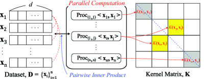
P1: Parallel Computation of Kernel Function. One property of kernel evaluation is the ability to induce parallel structures in the algorithm, such as computing kernel elements $K(\mathbf{x_{i}},\mathbf{x_{j}})=\phi(\mathbf{x_{i}})\cdot\phi(\mathbf{x_{j}})$ . Since evaluating kernel elements involves performing the same dot product structure over input vectors of the same size, HE can benefit from parallel computation of these kernel elements. For instance, in the basic HE model, (1) the server can perform concurrent computation of kernel elements during the pre-processing stage. (2) Alternatively, the client can compute the kernel elements and send the encrypted kernels to the server as alternative inputs, replacing the original encrypted data for further computation. Either way, the server can bypass the heavy multiplication in the pre-processing stage, thereby accelerating the overall kernel evaluation process (see Fig. 1).

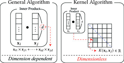
Refer to caption — Figure 1: (P1) *Parallel computation structure for evaluating kernel elements*. Expensive HE multiplications can be pre-computed in parallel during the initial stage for enhanced performance. Each kernel element evaluation can be assigned to a separate processor, enabling concurrent computation over the kernel matrix $\mathbf{K}$ .

P2: Dimensionless—Constant Time Complexity with respect to Dimension. A key feature of the kernel method in HE schemes is its dimensionless property. Generally, evaluating certain ML/STAT algorithms requires numerous inner products of vectors, each involving $d$ multiplications. Given the high computational cost of HE multiplications, this results in significant performance degradation. However, by employing the kernel method, we can circumvent the need for these dot products. Consequently, dimension-dependent computations are avoided during kernel evaluation, leading to a total time complexity that is constant with respect to the data dimension $d$ , unlike general algorithms, which have a linear dependency on $d$ (see Fig. 2).

III-C Example: $k$ -means Algorithm

The $k-$ means algorithm is an iterative process for finding optimal clusters. The algorithm deals with (1) cluster reassignment and (2) centroid update (see Fig. 3). The bottleneck is the cluster reassignment process that computes the distance $d(\mathbf{x}_{j},\bm{\mu}_{i})$ from each centroid $\bm{\mu}_{i}$ . Since evaluating the distance requires a dot product of the deviation from the centroid, $d$ multiplications are required for calculating each distance. Assuming that the algorithm converges in $t$ iteration, the total number of multiplications is $tnkd$ .

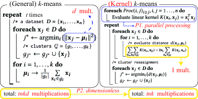
Using the kernel method and its properties, we can significantly improve the time performance of the circuit. First, we express the distance in terms of the kernel elements:

d(\mathbf{x}_{j},\bm{\mu}_{i})=\mathop{\sum\sum}_{\mathbf{x}_{a},\mathbf{x}_{b}\in g_{i}}K(\mathbf{x}_{a},\mathbf{x}_{b})-2n_{i}\sum\limits_{\mathbf{x}_{a}\in g_{i}}K(\mathbf{x}_{j},\mathbf{x}_{a})

(1)

where $n_{i}$ is the number of elements in the cluster $g_{i}\in\{g_{1},\dots,g_{k}\}$ . We verify that only one multiplication is performed in Eq. (1), which reduces the multiplications by a factor of $d$ from the general distance calculation. Therefore, the total number of multiplications in the kernel $k-$ means is $tnk$ (P2, dimensionless property), whereas $tnkd$ in the general method. Note that we can evaluate the kernel elements in parallel at the algorithm’s beginning, compensating for the $d$ multiplication time (P1, parallel structure).

Kernel Method—More Effective in the Encrypted Domain: $k-$ means Simulation. Based on algorithms in Fig. 3, we simulate the $k$ -means algorithm within different types of domains—plain, TFHE, CKKS, and B/FV—to demonstrate the effectiveness of the kernel method in the encrypted domain (see Fig. 4). We count the total number of additions and multiplications in $k-$ means; based on the HE parameter set and execution time in Table I, we compute the total simulation time with fixed parameters $t=10,k=3$ .

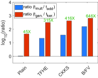
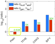
The result indicates that the kernel method is more effective in the encrypted domain. Fig. 4a shows that the kernel method has a significant speed-up when the time ratio of addition and multiplication is large. For instance, B/FV has a maximum speed-up of $645$ times, whereas plain kernel has $45$ times (CKKS: $416$ times, TFHE: $315$ times). Moreover, Fig. 4b demonstrates that depending on the parameter set, the kernel effect on the time performance can differ. For instance, B/FV has a speed-up of $35$ times in Fig. 4b.

Furthermore, the kernel can even have a negative impact on the execution time. For example, the plain kernel in Fig. 4b conversely decreases the total execution time by $53$ percent. This highlights the sensitivity of the plain kernel’s performance to variations. We provide actual experimental results regarding the kernel effect in Section VI.

III-D Benefits of the Kernel Method

Software-Level Optimization—Synergistic with Any HE Schemes or Libraries. The kernel method is synergistic with any HE scheme, amplifying the speed-up achieved by HE hardware accelerators since it operates at the software level. For instance, [11] uses GPUs at the hardware level to accelerate HE multiplication by 4.05 times in the CKKS scheme. When the kernel method is applied to evaluate the SVM of dimension 784 (single usage: 269 $\times$ ), it can increase acceleration by more than 1,076 times. Most current literature focuses on the hardware acceleration of each HE scheme. However, the kernel method does not compete with each accelerator; instead, it enhances the time performance of HE circuits.

Reusability of the Kernel Matrix. The kernel method enables the reusability of the kernel matrix, which can be employed in other kernel algorithms. The server can store both the dataset $\mathbf{D}$ and the kernel matrix $\mathbf{K}$ , eliminating the need to reconstruct inner products of data points. This results in faster computations and efficient resource utilization.

IV Kernel Trick and Asymptotic Complexities

This section analyzes the time complexities of general and kernel evaluations for ML/STAT algorithms. We first present a summary of the theoretical time complexities in Table II, followed by an illustration of how these complexities are derived. Note that the $k$ -means and $k$ -NN algorithms use a Boolean-based approach, while the remaining algorithms are implemented with an arithmetic HE scheme.

TABLE II: Comparison of Time Complexities in ML/STAT Algorithms

Algorithm	General TC	Kernel TC
SVM	$O(tn^{2}d)$	$O(tn^{2})$
PCA	$O(m^{2}+mt_{pow}+nm)$	$O(nr+rt_{pow}+3nt_{sqrt})$
$k$ -NN	$O(10ndl+6ndl^{2}+\Delta_{shared})$	$O(15nl+\Delta_{shared})$
$k$ -means	$O(6tnkdl^{2}+tnkdl)$	$O(11tn^{2}kl+3tnk^{2}l)$
Total Variance	$O(nd)$	$O(1)$
Distance	$O(d)$	$O(1)$
Norm	$O(d+3t_{sqrt})$	$O(3t_{sqrt})$
Similarity	$O(3d+3t_{sinv}+6t_{sqrt})$	$O(3t_{sinv}+6t_{sqrt})$

IV-A Arithmetic HE Construction

Matrix Multiplication and Linear Transformation. Halevi et al. [26] demonstrate efficient matrix and matrix-vector multiplication within HE schemes. Specifically, the time complexity for multiplying two $n\times n$ matrices is optimized to $O(n^{2})$ , while linear transformations are improved to $O(n)$ .

Dominant Eigenvalue: Power Iteration. The power iteration method [28] recursively multiplies a matrix by an initial vector until convergence. For a square matrix of degree $m$ , assuming $t_{pow}$ iterations, the time complexity is $O(mt_{pow})$ .

Square Root and Inverse Operation of Real Numbers. Wilkes’s iterative algorithm [29] approximates the square root operation with a complexity of $O(t_{sqrt})$ . Goldschmidt’s division algorithm approximates the inverse operation with a complexity of $O(t_{sinv})$ .

IV-A1 SVM

Kernel Trick. The main computation part of SVM is to find the optimal parameter $\bm{\alpha}=(\alpha_{1},\dots,\alpha_{n})$ to construct the optimal hyperplane $h^{*}(\mathbf{x})=\mathbf{w}^{T}\mathbf{x}+b$ . For optimization, we use SGD algorithm that iterates over the following gradient update rule: $\alpha_{k}=\alpha_{k}+\eta(1-y_{k}\sum\limits_{i=1}^{n}\alpha_{i}y_{i}\mathbf{x}_{i}^{T}\mathbf{x}_{j})$ .

The kernel trick for SVM is a replacement of $\mathbf{x}_{i}^{T}\mathbf{x}_{j}$ with a linear kernel element $K(\mathbf{x}_{i},\mathbf{x}_{j})$ . Thus, we compute $\alpha_{k}=\alpha_{k}+\eta(1-y_{k}\sum\limits_{i=1}^{n}\alpha_{i}y_{i}K(\mathbf{x}_{i},\mathbf{x}_{j}))$ for the kernel evaluation.

(1) General Method. The gradient update rule for $\alpha_{k}$ requires $n(d+2)+1=O(nd)$ multiplications. For the complete set of $\bm{\alpha}$ and assuming that the worst-case of convergence happens in $t$ iterations, the total time complexity is $O(tn^{2}d)$ .

(2) Kernel Method. The kernel trick bypasses inner products, which requires $d$ multiplications. Hence, it requires $2n+1=O(n)$ multiplications for updating $\alpha_{k}$ ( $O(n^{2})$ for $\bm{\alpha}$ ). Therefore, the total time complexity is $O(tn^{2})$ .

IV-A2 PCA

Kernel Trick. Suppose $\lambda_{1}$ is the dominant eigenvalue with the corresponding eigenvector $\mathbf{u}_{1}$ of the covariance matrix $\bm{\Sigma}$ . Then, the eigenpair $(\lambda_{1},\mathbf{u}_{1})$ satisfies $\bm{\Sigma}\mathbf{u}_{1}=\lambda_{1}\mathbf{u}_{1}$ . Since $\bm{\Sigma}=\frac{1}{n}\sum\limits_{i=1}^{n}\mathbf{x}_{i}\mathbf{x}_{i}^{T}$ , we can express $\mathbf{u}_{1}=\sum\limits_{i=1}^{n}c_{i}\mathbf{x}_{i}$ where $c_{i}=\frac{\mathbf{x}_{i}^{T}\mathbf{u}_{1}}{n\lambda_{1}}$ . Plugging in the formulae for $\Sigma$ and $\bm{\mu}_{1}$ and multiplying $\mathbf{x}_{k}^{T}$ on both sides yield: $\sum\limits_{i=1}^{n}\mathbf{x}_{k}^{T}\mathbf{x}_{i}\sum\limits_{j=1}^{n}c_{j}\mathbf{x}_{i}^{T}\mathbf{x}_{j}=n\lambda_{1}\sum\limits_{i=1}^{n}c_{i}\mathbf{x}_{k}^{T}\mathbf{x}_{i}$ for all $\mathbf{x}_{k}\in\textbf{D}$ . By substituting inner products with the corresponding kernel elements $K(\cdot,\cdot)$ , we derive the following equation expressed in terms of the kernel elements:

\sum\limits_{i=1}^{n}K(\mathbf{x}_{k},\mathbf{x}_{i})\sum\limits_{j=1}^{n}c_{j}K(\mathbf{x}_{i},\mathbf{x}_{j})=n\lambda_{1}\sum\limits_{i=1}^{n}c_{i}K(\mathbf{x}_{k},\mathbf{x}_{i}).

Further simplification yields $\mathbf{K}\mathbf{c}=(n\lambda_{1})\mathbf{c}$ , where $\mathbf{c}$ is an eigenvector of the kernel matrix $\mathbf{K}$ . Thus, a reduced basis element $\bm{\mu}_{i}$ is derived by scaling $\mathbf{c}_{i}$ with $\sqrt{\lambda_{i}\mathbf{c}_{i}^{T}\mathbf{c}_{i}}$ .

Comparison of Complexities. Both general and kernel methods require the computation of eigenvalues and eigenvectors using the power iteration method for the covariance matrix $\bm{\Sigma}$ and kernel matrix $\mathbf{K}$ .

(1) General Method. This algorithm involves one matrix multiplication, power iteration, and $n$ matrix-vector multiplications. The time complexity is $O(m^{2}+mt_{pow}+nm)$ , where $m=\text{max}(n,d)$ .

(2) Kernel Method. This algorithm involves power iteration, $r$ normalizations (square root), and $rn$ inner-products. The time complexity is $O(nt_{pow}+3rt_{sqrt}+nr)$ .

IV-A3 Total Variance

Kernel Trick. The linear kernel trick simplifies the normal variance formula by expressing it in terms of dot products:

\displaystyle TV=\frac{1}{n}\sum\limits_{i=1}^{n}\lVert\mathbf{x}_{i}-\bm{\mu}\rVert^{2}=\frac{1}{n}\sum\limits_{i=1}^{n}K(\mathbf{x}_{i},\mathbf{x}_{i})-\frac{1}{n^{2}}\sum\limits_{i=1}^{n}\sum\limits_{j=1}^{n}K(\mathbf{x}_{i},\mathbf{x}_{j})

where the second equality holds by substituting $\bm{\mu}=\frac{1}{n}\sum_{i=1}^{n}\mathbf{x}_{i}$ .

(1) General Method. This requires $n$ dot products of deviations; the time complexity is $O(nd)$ .

(2) Kernel Method. The kernel trick for total variance bypasses dot products, resulting in a time complexity of $O(1)$ .

IV-A4 Distance / Norm

Kernel trick. We can apply the linear kernel trick on distance $\mathcal{d}(\mathbf{x}_{i},\mathbf{x}_{j})=\lVert\mathbf{x}_{i}-\mathbf{x}_{j}\rVert^{2}$ :

\displaystyle\begin{split}\mathcal{d}(\mathbf{x}_{i},\mathbf{x}_{j})&=\lVert\mathbf{x}_{i}\rVert^{2}-2\mathbf{x}_{i}^{T}\mathbf{x}_{j}+\lVert\mathbf{x}_{j}\rVert^{2}\\ &=K(\mathbf{x}_{i},\mathbf{x}_{i})-2K(\mathbf{x}_{i},\mathbf{x}_{j})+K(\mathbf{x}_{j},\mathbf{x}_{j}).\end{split}

(1) General Method. The general distance formula requires $O(d)$ for evaluating a dot product. Moreover, norm operation entails additional square root operation; hence, $O(d+3t_{sqrt})$ .

(2) Kernel Method. The kernel method necessitates only addition and subtraction requiring $O(1)$ . Likewise, kernelized norm involves the square root operation; thus, $O(3t_{sqrt})$ .

IV-A5 Similarity

Kernel Trick. Applying the linear kernel trick to cosine similarity formula, we have

sim(\mathbf{x}_{i},\mathbf{x}_{j})=\frac{\mathbf{x}_{i}\cdot\mathbf{x}_{j}}{\lVert\mathbf{x}_{i}\rVert\lVert\mathbf{x}_{j}\rVert}=\frac{K(\mathbf{x}_{i},\mathbf{x}_{j})}{\sqrt{K(\mathbf{x}_{i},\mathbf{x}_{i})}\sqrt{K(\mathbf{x}_{j},\mathbf{x}_{j})}}.

(1) General Method. We compute three dot products, one multiplication, one inverse of a scalar, and two square root operations for computing the general cosine similarity. Hence, it requires $O(3d+3t_{sinv}+6t_{sqrt})$ .

(2) Kernel Method. We can bypass the evaluation of the three inner products using the kernel method. Thus, the total time complexity is $O(3t_{sinv}+6t_{sqrt})$ .

IV-B Boolean-based HE Construction

$k$ -means and $k$ -NN Boolean Construction. Performing $k$ -means and $k$ -NN in the encrypted domain requires functionalities beyond addition and multiplication, such as comparison operations. In the $k$ -means algorithm, it is essential to evaluate the minimum encrypted distance to label data based on proximity to each cluster’s encrypted mean. Similarly, $k$ -NN necessitates evaluating the maximum encrypted labels given the encrypted distances to all data points. Detailed algorithms for $k$ -means and $k$ -NN are provided in the Appendix.

Time Complexity for TFHE Circuit Evaluation. We measure the algorithms’ performance by counting the total number of binary gates for exact calculation. Boolean gates such as XOR, AND, and OR take twice the time of a single MUX gate [14]. We assume that the TFHE ciphertext is an encryption of an $l$ -bit fixed-point number, with $l/2$ bits for decimals, $(l/2-1)$ bits for integers, and $1$ bit for the sign bit. Table III presents the time complexity of fundamental TFHE operations used throughout the paper.

TABLE III: Time complexity of TFHE operations used in the paper

	TFHE Basic Operation
	Comparison	argmin / argmax	Add / Subt.	Multiplication	Absolute Value	Two’s Complement	Division
$\#$ (Binary Gate)	$3l$	$k(k-1)(3l+1)$	$5l-3$	$6l^{2}+15l-6$	$4l-1$	$2l-1$	$\frac{27}{2}l^{2}-\frac{3}{2}l+1$

IV-B1 $k$ -means

Kernel Trick. Let $\mathcal{d}_{ij}$ denote the distance from data point $\mathbf{x}_{i}$ to the mean of cluster $g_{j}$ .

\mathcal{d}_{ij}=\lVert\mathbf{x}_{i}-\bm{\mu}_{j}\rVert^{2}=\mathbf{x}_{i}^{T}\mathbf{x}_{i}-\frac{1}{n_{j}}\sum_{\mathbf{x}_{a}\in g_{j}}\mathbf{x}_{i}^{T}\mathbf{x}_{a}+\frac{1}{n_{j}^{2}}\sum_{\mathbf{x}_{a},\mathbf{x}_{b}\in g_{j}}\mathbf{x}_{a}^{T}\mathbf{x}_{b}

where $n_{j}$ is the number of elements in cluster $g_{j}$ . Applying the linear kernel trick, we can compute $\mathcal{d}_{ij}$ using kernel elements:

\mathcal{d}_{ij}=K(\mathbf{x}_{i},\mathbf{x}_{i})-\frac{1}{n_{j}}\sum_{\mathbf{x}_{a}\in g_{j}}K(\mathbf{x}_{i},\mathbf{x}_{a})+\frac{1}{n_{j}^{2}}\sum_{\mathbf{x}_{a},\mathbf{x}_{b}\in g_{j}}K(\mathbf{x}_{a},\mathbf{x}_{b})

Further simplification yields the objective function:

j^{*}=\underset{j}{\text{argmin}}\left\{-n_{j}\sum_{\mathbf{x}_{a}\in g_{j}}K(\mathbf{x}_{i},\mathbf{x}_{a})+\sum_{\mathbf{x}_{a},\mathbf{x}_{b}\in g_{j}}K(\mathbf{x}_{a},\mathbf{x}_{b})\right\}

(2)

where the common factor $K(\mathbf{x}_{i},\mathbf{x}_{i})$ and divisions are omitted for efficiency.

(1) General Method. The $k$ -means algorithm involves four steps: computing distances $\mathcal{d}_{ij}$ , labeling $\mathbf{x}_{i}$ , forming labeled dataset $\textbf{D}^{(i)}$ , and calculating cluster means $\bm{\mu}_{j}$ . The total complexity of $k$ -means is asymptotically $O(6tnkdl^{2}+tnkdl)$ , assuming $t$ iterations until convergence.

(2) Kernel Method. The kernel $k$ -means algorithm involves four steps: computing the labeled kernel matrix $K^{(j)}$ , counting the number of elements $\mathcal{n}_{j}$ in each cluster, computing distances $\mathcal{d}_{ij}$ , and labeling $\mathbf{x}_{i}$ . The total complexity of kernel $k$ -means is asymptotically $O(11tn^{2}kl+3tnk^{2}l)$ , assuming $t$ iterations until convergence.

IV-B2 $k$ -NN

Kernel Trick. The linear kernel trick can be applied to the distance $\mathcal{d}_{i}$ in $k$ -NN:

\begin{split}\mathcal{d}_{i}=\lVert\mathbf{x}-\mathbf{x}_{i}\rVert^{2}&=\mathbf{x}^{T}\mathbf{x}-2\mathbf{x}^{T}\mathbf{x}_{i}+\mathbf{x}_{i}^{T}\mathbf{x}_{i}\\ &=K(\mathbf{x},\mathbf{x})-2K(\mathbf{x},\mathbf{x}_{i})+K(\mathbf{x}_{i},\mathbf{x}_{i}).\end{split}

For computational efficiency, we simplify $\mathcal{d}_{i}$ by removing the common kernel element $K(\mathbf{x},\mathbf{x})$ :

\mathcal{d}_{i}=-2K(\mathbf{x},\mathbf{x}_{i})+K(\mathbf{x}_{i},\mathbf{x}_{i}).

(3)

Comparison of Complexities. Both $k$ -NN algorithms share the same processes: sorting, counting, and finding the majority label. Specifically, sorting requires $(n-1)^{2}$ swaps, with each swap involving 4 MUX gates and one comparison circuit, resulting in a complexity of $11(n-1)^{2}l$ . Counting elements in each class requires $ks$ comparisons and additions, with a complexity of $ks(8l-3)$ . Finding the majority index among $s$ labels has a complexity of $s(s-1)(3l+1)$ . Thus, the shared complexity is $O(11n^{2}l+8ksl+3s^{2}l)$ , denoted as $\Delta_{shared}$ .

(1) General Method. Computing $\mathcal{d}_{i}=\lVert\mathbf{x}-\mathbf{x}_{i}\rVert^{2}$ involves $d$ subtractions, $d$ multiplications, and $d-1$ additions, resulting in a total complexity of $O(10ndl+6ndl^{2})$ . Including the shared process, the total complexity is $O(10ndl+6ndl^{2}+\Delta_{shared})$ .

(2) Kernel Method. Using Eq. (3), $\mathcal{d}_{i}$ is computed with one addition and two subtractions per element, totaling $3n$ additions. Including the shared process, the total complexity is $O(15nl+\Delta_{shared})$ .

V Experiment

V-A Evaluation Metric

We aim to evaluate the effectiveness of the kernel method in various ML/STAT algorithms using the following metrics.

(1) Kernel Effect in HE. Let $t_{gen}$ and $t_{ker}$ denote the execution times for the general and kernel methods, respectively. The kernel effectiveness or speed-up is evaluated by the ratio:

EFF=\frac{t_{gen}}{t_{ker}}.

(2) Kernel Effect Comparison: Plain and HE. Let $t_{gen}^{PL}$ and $t_{ker}^{PL}$ represent the execution times for the general and kernel methods in the plain domain. Similarly, let $t_{gen}^{HE}$ and $t_{ker}^{HE}$ represent the execution times in the HE domain. The effectiveness of the kernel methods in both domains can be compared by their respective ratios: $EFF^{PL}$ and $EFF^{HE}$ .

V-B Experiment Setting

Environment. Experiments were conducted on an Intel Core i7-7700 8-Core 3.60 GHz, 23.4 GiB RAM, running Ubuntu 20.04.5 LTS. We used TFHE version 1.1 for Boolean-based HE and CKKS from OpenFHE [18] for arithmetic HE.

Dataset and Implementation Strategy. We used a randomly generated dataset of $n=10$ data points with dimensions in $[n/2,3n/2]$ . The dataset is intentionally small due to the computational time required for logic-gates in TFHE. For example, $k$ -means with parameters ( $n,d=10$ ) under the TFHE scheme takes 8,071 seconds. Despite the small dataset, this work aligns with on-going efforts like Google’s Transpiler [27] and its extension HEIR, which use TFHE for practical HE circuit construction. Employing the kernel method can significantly enhance scalability and efficiency.

Parameter Setting. Consistent parameters were used for both the general and kernel methods across all algorithms.

(1) TFHE Construction. TFHE constructions were set to a 110-bit security level⁶⁶6Initial tests at 128-bit security were revised due to recent attacks demonstrating a lower effective security level., with 16-bit message precision.

(2) CKKS Construction. CKKS constructions used a 128-bit security level and a leveled approach to avoid bootstrapping. Parameters ( $N,\Delta,L$ ) were pre-determined to minimize computation time (see Table IV).

(3) $k$ -means and $k$ -NN. For the experiments, $k=3$ and $s=2$ were used for $k$ -means, and $k=3$ for $k$ -NN.

TABLE IV: Parameter setting for CKKS implementation

	$\lambda$	RingDim $N$	ScalingMod $\Delta$	MultDepth $L$
SVM	$128$	$2^{16}$	$2^{50}$	$110$
PCA	$128$	$2^{16}$	$2^{50}$	$39$
Variance	$128$	$2^{16}$	$2^{50}$	$33$
Distance	$128$	$2^{16}$	$2^{50}$	$33$
Norm	$128$	$2^{16}$	$2^{50}$	$33$
Similarity	$128$	$2^{16}$	$2^{50}$	$50$

VI Results and Analysis

VI-A Kernel Effect in the Encrypted Domain

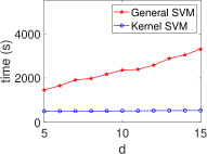
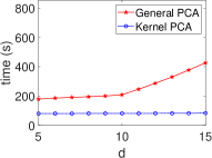
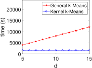
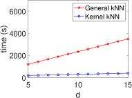
Kernel Method in ML/STAT: Acceleration in HE Schemes. Fig. 5 demonstrates the stable execution times of kernel methods in ML algorithms within encrypted domains, contrasting with the linear increase observed in general methods. This consistency in both CKKS and TFHE settings aligns with our complexity analysis in Table II, improving computational efficiency for algorithms such as SVM, PCA, $k$ -means, and $k$ -NN. Notably, for general PCA, we observe a linear time increase for $d<n$ and a rapid rise as $O(m^{2})$ for $d>n$ due to the quadratic complexity of evaluating the covariance matrix $\bm{\Sigma}=\textbf{D}^{T}\textbf{D}$ .

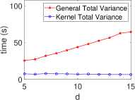
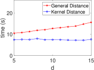
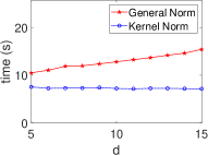
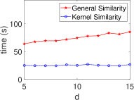
Fig. 6 shows that the kernel method consistently outperforms general approaches in STAT algorithms within HE schemes. The kernel method maintains stable execution times across various statistical algorithms, unlike the linearly increasing times of general methods as data dimension grows. This aligns with our complexity calculations (Table II), highlighting the kernel method’s efficiency in encrypted data analysis. The dimensionless property of the kernel method makes it a powerful tool for high-dimensional encrypted data analysis, enabling efficient computations in complex settings.

Kernelization Time (Pre-Processing Stage). Kernelization occurs during preprocessing, with kernel elements computed in parallel. Although not included in the main evaluation duration, kernelization time is minimal, constituting less than 0.05 of the total evaluation time. For instance, in SVM, kernel generation accounts for only 0.02 of the total evaluation time (10.82 seconds of 509.91 seconds). Additionally, the reusability of kernel elements in subsequent applications further reduces the need for repeated computations.

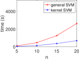
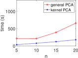
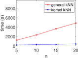
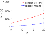
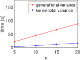
Kernel Method Outperforms with Increasing Data. We present the execution time of four ML algorithms (SVM, PCA, $k$ -NN, $k$ -means) and the total variance in the STAT algorithm, with respect to varying numbers of data ( $n=5,10,15,20$ ) at a fixed dimension ( $d=10$ ), as shown in Fig. 7. Our results demonstrate that the kernel method consistently outperforms the general method in terms of execution time, even as the number of data increases. This aligns with our complexity table (see Table 3), where general SVM and PCA show a quadratic increase, while $k$ -NN, $k$ -means, and total variance increase linearly.

VI-B Kernel Effect Comparison: Plain vs HE

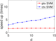
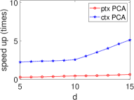
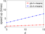
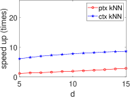
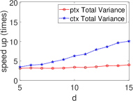
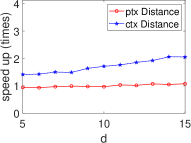
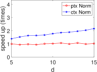
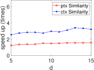
Significant Kernel Effect in the HE Domain. Our experiments demonstrate a more substantial kernel effect in the HE domain compared to the plain domain for both ML and STAT algorithms. This effect is consistently observed across algorithms (see Fig. 8 and Fig. 9). For example, the kernel effect in SVM within HE amplifies performance by 2.95-6.26 times, compared to 1.58-1.69 times in the plain domain, across dimensions 5-15. This enhanced performance is due to the kernel method’s ability to reduce heavy multiplicative operations, a significant advantage in HE where multiplication is more time-consuming than addition (see Section III).

VII Conclusion

This paper introduces the kernel method as an effective optimizer for homomorphic circuits in ML/STAT applications, applicable across various HE schemes. We systematically analyze the kernel optimization and demonstrate its effectiveness through complexity analysis and experiments. Our results show significant performance improvements in the HE domain, highlighting the potential for widespread use in secure ML/STAT applications.

References

[1] C. Gentry, ”Fully homomorphic encryption using ideal lattices,” in Proc. 41st Annu. ACM Symp. Theory Comput., 2009, pp. 169–178.
[2] A. Kim, Y. Song, M. Kim, K. Lee, and J. H. Cheon, ”Logistic regression model training based on the approximate homomorphic encryption,” BMC Med. Genomics, vol. 11, no. 4, pp. 23–31, 2018.
[3] H. Chen, R. Gilad-Bachrach, K. Han, Z. Huang, A. Jalali, K. Laine, and K. Lauter, ”Logistic regression over encrypted data from fully homomorphic encryption,” BMC Med. Genomics, vol. 11, no. 4, pp. 3–12, 2018.
[4] Y. Aono, T. Hayashi, L. T. Phong, and L. Wang, ”Scalable and secure logistic regression via homomorphic encryption,” in Proc. Sixth ACM Conf. Data Appl. Secur. Priv., 2016, pp. 142–144.
[5] E. Crockett, ”A low-depth homomorphic circuit for logistic regression model training,” Cryptology ePrint Archive, 2020.
[6] F. Boemer, A. Costache, R. Cammarota, and C. Wierzynski, ”nGraph-HE2: A high-throughput framework for neural network inference on encrypted data,” in Proc. 7th ACM Workshop Encrypted Comput. & Appl. Homomorphic Cryptogr., 2019, pp. 45–56.
[7] A. Brutzkus, R. Gilad-Bachrach, and O. Elisha, ”Low latency privacy preserving inference,” in Int. Conf. Mach. Learn., 2019, pp. 812–821.
[8] R. Gilad-Bachrach, N. Dowlin, K. Laine, K. Lauter, M. Naehrig, and J. Wernsing, ”Cryptonets: Applying neural networks to encrypted data with high throughput and accuracy,” in Int. Conf. Mach. Learn., 2016, pp. 201–210.
[9] W. Jung, S. Kim, J. H. Ahn, J. H. Cheon, and Y. Lee, ”Over 100x faster bootstrapping in fully homomorphic encryption through memory-centric optimization with GPUs,” IACR Trans. Cryptogr. Hardw. Embed. Syst., pp. 114–148, 2021.
[10] J. H. Cheon, A. Kim, M. Kim, and Y. Song, ”Homomorphic encryption for arithmetic of approximate numbers,” in Int. Conf. Theory Appl. Cryptol. Inf. Secur., Springer, 2017, pp. 409–437.
[11] W. Jung, E. Lee, S. Kim, J. Kim, N. Kim, K. Lee, C. Min, J. H. Cheon, and J. H. Ahn, ”Accelerating fully homomorphic encryption through architecture-centric analysis and optimization,” IEEE Access, vol. 9, pp. 98772–98789, 2021.
[12] I. Chillotti, M. Joye, and P. Paillier, ”Programmable bootstrapping enables efficient homomorphic inference of deep neural networks,” in Int. Symp. Cyber Secur. Cryptogr. Mach. Learn., Springer, 2021, pp. 1–19.
[13] I. Chillotti, N. Gama, M. Georgieva, and M. Izabachene, ”Faster fully homomorphic encryption: Bootstrapping in less than 0.1 seconds,” in Adv. Cryptol.–ASIACRYPT, 2016, pp. 3–33.
[14] I. Chillotti, N. Gama, M. Georgieva, and M. Izabachène, ”TFHE: Fast Fully Homomorphic Encryption over the Torus,” J. Cryptol., vol. 33, no. 1, pp. 34–91, 2020.
[15] M. J. Zaki and W. Meira, Data Mining and Analysis: Fundamental Concepts and Algorithms. Cambridge University Press, 2014.
[16] Part Guide, ”Intel® 64 and ia-32 architectures software developer’s manual,” Vol. 3B: System Programming Guide, Part, vol. 2, no. 11, 2011.
[17] L. Deng, ”The MNIST database of handwritten digit images for machine learning research,” IEEE Signal Process. Mag., vol. 29, no. 6, pp. 141–142, 2012.
[18] A. Al Badawi et al., ”OpenFHE: Open-Source Fully Homomorphic Encryption Library,” in Proc. 10th Workshop Encrypted Comput. & Appl. Homomorphic Cryptogr., 2022, pp. 53–63.
[19] O. Regev, ”On lattices, learning with errors, random linear codes, and cryptography,” J. ACM, vol. 56, no. 6, pp. 1–40, 2009.
[20] D. Stehlé, R. Steinfeld, K. Tanaka, and K. Xagawa, ”Efficient public key encryption based on ideal lattices,” in ASIACRYPT, 2009, pp. 617–640.
[21] Z. Brakerski, C. Gentry, and V. Vaikuntanathan, ”(Leveled) fully homomorphic encryption without bootstrapping,” ACM Trans. Comput. Theory, vol. 6, no. 3, pp. 1–36, 2014.
[22] J. Fan and F. Vercauteren, ”Somewhat practical fully homomorphic encryption,” Cryptology ePrint Archive, 2012.
[23] C. Gentry, A. Sahai, and B. Waters, ”Homomorphic encryption from learning with errors: Conceptually-simpler, asymptotically-faster, attribute-based,” in Annu. Cryptol. Conf., 2013, pp. 75–92.
[24] L. Ducas and D. Micciancio, ”FHEW: bootstrapping homomorphic encryption in less than a second,” in Annu. Int. Conf. Theory Appl. Cryptogr. Tech., 2015, pp. 617–640.
[25] B. Schölkopf, A. J. Smola, and F. Bach, Learning with Kernels: Support Vector Machines, Regularization, Optimization, and Beyond. MIT Press, 2002.
[26] S. Halevi and V. Shoup, ”Faster homomorphic linear transformations in HElib,” in Annu. Int. Cryptol. Conf., 2018, pp. 93–120.
[27] S. Gorantala, R. Springer, S. Purser-Haskell, W. Lam, R. Wilson, A. Ali, E. P. Astor, I. Zukerman, S. Ruth, C. Dibak, et al., ”A general purpose transpiler for fully homomorphic encryption,” arXiv preprint arXiv:2106.07893, 2021.
[28] G. H. Golub and H. A. Van der Vorst, ”Eigenvalue computation in the 20th century,” J. Comput. Appl. Math., vol. 123, no. 1–2, pp. 35–65, 2000.
[29] M. V. Wilkes, D. J. Wheeler, and S. Gill, The Preparation of Programs for an Electronic Digital Computer: With special reference to the EDSAC and the Use of a Library of Subroutines. Addison-Wesley Press, 1951.

Appendix A ML / STAT

Appendix B $k-$ means and $k-$ NN: Boolean Construction

B-A Boolean-based HE Construction: $k$ -means

(1) General Method. Constructing the $k$ -means circuit in the encrypted domain presents a primary challenge: the iterative update of encrypted labels $\bm{\mathcal{l}}$ in each iteration.

l_{i}=\underset{j}{\text{argmin}}\{\mathcal{d}_{ij}\}_{j=1}^{k}.

(4)

This involves two key tasks: 1) labeling data $x_{i}$ using Eq. (4), and 2) computing the average value for each cluster $g_{i}$ based on the encrypted labels.

Issue 1: Labeling Data. We solve Eq. (4) using the TFHE.LEQ $(\mathsf{ct_{1}},\mathsf{ct_{2}})$ comparison operation. This operation returns $\mathsf{Enc}(1)$ if $\mathsf{ct_{1}}$ is less than or equal to $\mathsf{ct_{2}}$ , and $\mathsf{Enc}(0)$ otherwise. Algorithm 1 determines the index of the minimum value from a set of encrypted ciphertexts $\{\mathcal{d}_{i}\}_{i=1}^{k}$ . The output is a binary ciphertext $\bm{\mathcal{l}}^{*}=(\mathcal{l}_{1},\dots,\mathcal{l}_{k})$ , where a non-zero $\mathcal{l}_{j}$ indicates the label corresponding to $\mathbf{x}_{i}$ .

2for $i=1,\dots,k$ do

\mathcal{l}_{i}\leftarrow\mathsf{Enc}(1)

4 for $j=1,\dots,k$ do

\mathcal{t}\leftarrow

\underset{j\neq i}{\text{TFHE.LEQ}(\mathcal{d}_{i},\mathcal{d}_{j})}

\mathcal{l}_{i}\leftarrow

TFHE.AND(

\mathcal{l}_{i},t

)

\bm{\mathcal{l}}^{*}\leftarrow(\mathcal{l}_{1},\dots,\mathcal{l}_{k})

Algorithm 1 TFHE.argmin_i

\{\mathcal{d}_{i}\}_{i=1,\dots,k}

Issue 2: Computing Average Value. Identifying the data $\mathbf{x}_{i}$ in a specific group $g_{j}$ using encrypted labels $\bm{\mathcal{l}}_{i}$ is challenging. We address this by extracting cluster data $\mathbf{D}^{(j)}$ , setting non-belonging data to zero through an AND operation between each label $l_{ij}$ and its respective data $\mathbf{x}_{i}$ (see Algorithm 2).

\mathbf{x}_{j}\leftarrow\mathbf{x}_{j}\text{ or }\mathbf{x}_{j}\leftarrow\mathsf{Enc}(0)\text{ by label }\mathcal{l}_{ji}

3foreach $\mathbf{x}_{j}=(x_{j1},\dots,x_{jl})\in\mathbf{D}$ do

x_{jk}\leftarrow

TFHE.AND(

\mathcal{l}_{ji},x_{jk}),k=1,\dots,l

Algorithm 2 TFHE.GetClusterData(

\mathbf{D}

\mathcal{L}

)

With $\mathbf{D}^{(j)}$ identified, the mean $\bm{\mu}_{j}$ for each cluster is computed by summing all elements in $\mathbf{D}^{(j)}$ and dividing by the number of elements in the class $g_{j}$ . The number of elements in each class is obtained by summing the encrypted label $\mathcal{l}_{ji}$ for all $\mathbf{x}_{i}\in\mathbf{D}$ (see Algorithm 3).

2for $i=1,\dots,k$ do

\mathbf{D}^{(i)}\leftarrow

TFHE.GetClusterData(

\textbf{D},\bm{\mathcal{L}}

i

)

4 for $\mathbf{x}_{j}^{\prime}\in\mathbf{D}^{(i)}$ do

\mathcal{n}_{i}\leftarrow\sum\limits_{i=1}^{n}{\mathcal{l}_{i1}}

, and

\bm{\mu}_{i}\leftarrow\frac{1}{\mathcal{n}_{i}}\sum\limits_{j=1}^{n}\mathbf{x}_{j}^{\prime}

Algorithm 3 TFHE.ClusterMean(D,

\bm{\mathcal{L}}

)

/* parallel compute linear kernel */

\bm{\mathcal{L}}\leftarrow\{\bm{\mathcal{l}}_{i}|\bm{\mathcal{l}}_{i}=\mathsf{Enc}(a\overset{\$}{\leftarrow}\{1,\dots,k\}),i=1,\dots,n\}

4repeat

6 for $i=1,\dots,n$ do

8 for $j=1,\dots,k$ do

\textbf{K}^{(j)}\leftarrow

TFHE.GetClusterData(

\textbf{K},\bm{\mathcal{L}}_{i}

)

\mathcal{n}_{j}\leftarrow\sum\limits_{s=1}^{n}l_{sj}

\mathcal{p}\leftarrow\sum\limits_{a=1}^{n}\sum\limits_{b=1}^{n}\textbf{K}^{(j)}(\mathbf{x}_{a},\mathbf{x}_{b})

\mathcal{q}\leftarrow-2\mathcal{n}_{j}\sum\limits_{a=1}^{n}\textbf{K}^{(j)}(\mathbf{x}_{a},\mathbf{x}_{b})

\mathcal{d}_{j}\leftarrow\mathcal{p}+\mathcal{q}

\bm{\mathcal{l}}_{i}\leftarrow

TFHE.argmin

{}_{j}\{\mathcal{d}_{j}\}_{j=1,\dots,k}

18until $t$ times

Algorithm 4 TFHE.Kernel

k

-means(D,

k

t

)

(2) Kernel Method. Kernel $k$ -means reduces to solving Eq. (2). Directly solving partial sums from the kernel matrix is infeasible due to encrypted labels. Therefore, we proceed as follows (see Algorithm 4 for the complete kernel evaluation):

•

Obtain cluster-specific kernel $K^{(j)}$ , where $K^{(j)}(\mathbf{x}_{a},\mathbf{x}_{b})$ equals $K(\mathbf{x}_{a},\mathbf{x}_{b})$ if both $\mathbf{x}_{a},\mathbf{x}_{b}\in g_{j}$ ; otherwise, it is zero.
•

Compute the partial sums from Eq. (2) using the cluster-specific kernel $K^{(j)}$ .

Proc. 1: Cluster-specific Kernel. We obtain $K^{(j)}$ using $\mathcal{l}^{*}_{ij}$ and AND gates:

	$\displaystyle\mathcal{t}$	$\displaystyle\leftarrow\text{TFHE.AND}(\mathcal{l}^{*}_{aj},\mathcal{l}_{bj}),$
	$\displaystyle K^{(j)}(\mathbf{x}_{a},\mathbf{x}_{b})[s]$	$\displaystyle\leftarrow\text{TFHE.AND}(\mathcal{t},K(\mathbf{x}_{a},\mathbf{x}_{b})[s])$

where $\mathcal{t}$ is $\mathsf{Enc}(1)$ if both $\mathbf{x}_{a}$ and $\mathbf{x}_{b}$ belong to $g_{j}$ .

Proc. 2: Partial Sum Evaluation. We compute over $n\geq n_{j}$ elements in $K^{(j)}$ :

	$\displaystyle\sum_{\mathbf{x}_{a}\in g_{j}}K(\mathbf{x}_{i},\mathbf{x}_{a})$	$\displaystyle=\sum_{a=1}^{n}K^{(j)}(\mathbf{x}_{i},\mathbf{x}_{a})$
	$\displaystyle\sum_{\mathbf{x}_{a},\mathbf{x}_{b}\in g_{j}}K(\mathbf{x}_{a},\mathbf{x}_{b})$	$\displaystyle=\sum_{b=1}^{n}\sum_{a=1}^{n}K^{(j)}(\mathbf{x}_{a},\mathbf{x}_{b})$

B-B Boolean-based HE construction: $k-$ NN

(1) General Method: The $k$ -NN algorithm involves 1) sorting, 2) counting, and 3) finding the majority label among encrypted data. We address the issues as follows.

Issue 1: Sorting. We use the TFHE.minMax function, detailed in Algorithm 5, to arrange a pair of ciphertexts $\mathsf{ct_{1}},\mathsf{ct_{2}}$ in ascending order using the TFHE.LEQ operation. By using $\mathcal{t}$ and its negation $\sim\mathcal{t}$ as selectors in a MUX gate, we obtain the ordered pair $(\mathsf{ct}_{\text{min}},\mathsf{ct}_{\text{max}})$ .

\mathcal{t}\leftarrow

TFHE.LEQ(

\mathsf{ct}_{1},\mathsf{ct}_{2}

\sim\mathcal{t}\leftarrow

TFHE.NOT(

\mathcal{t}

)

3for $j=1,\dots,r$ do

\mathsf{ct}_{j}^{min}\leftarrow

TFHE.MUX(

\mathcal{t}

\mathsf{ct}_{1j}

\mathsf{ct}_{2j}

)

\mathsf{ct}_{j}^{max}\leftarrow

TFHE.MUX(

\sim\mathcal{t}

\mathsf{ct}_{1j}

\mathsf{ct}_{2j}

)

\mathcal{l}_{j}^{min}\leftarrow

TFHE.MUX(

\mathcal{t}

\mathcal{l}_{1j}

\mathcal{l}_{2j}

)

\mathcal{l}_{j}^{max}\leftarrow

TFHE.MUX(

\sim\mathcal{t}

\mathcal{l}_{1j}

\mathcal{l}_{2j}

)

Algorithm 5 TFHE.minMax(

(\mathsf{ct}_{1},\mathcal{l}_{1}),(\mathsf{ct}_{2},\mathcal{l}_{2})

)

By employing the TFHE.minMax function, Algorithm 6 executes the Bubblesort algorithm, yielding a sorted sequence $\{d_{i}^{*}\}_{i=1}^{n}$ in ascending order, with their respective labels $\mathcal{l}_{i}^{*}$ .

\mathcal{a}_{j}=(\mathcal{d}_{j},\mathcal{l}_{j})

3repeat

5 for $j=1,\dots,n-1$ do

(\mathcal{a}_{j},\mathcal{a}_{j+1})\leftarrow

TFHE.minMax(

\mathcal{a}_{j},\mathcal{a}_{j+1}

)

9until $n-1$ times

Algorithm 6 TFHE.BubbleSort(

\{\mathcal{d}_{i}\}_{i=1}^{n},\bm{\mathcal{l}}

)

Issue 2: Counting. From the sorted distances $\{d_{i}^{*}\}_{i=1}^{n}$ and respective labels $\{\mathcal{l}_{i}^{*}\}_{i=1}^{n}$ , we count the number of elements in each class $g_{j}$ among the $k$ nearest neighbors. We repeatedly use the TFHE.EQ comparison, which outputs $\mathsf{Enc}(1)$ if two input ciphertexts are equal (see Algorithm 7).

2for $i=1,\dots,s$ do

\mathcal{n}_{i}\leftarrow\mathsf{Enc}(0)

4 for $j=1,\dots,k$ do

\mathcal{t}\leftarrow

TFHE.EQ(

\mathsf{Enc}(i),\mathcal{l}^{*}_{j}

)

\mathcal{n}_{i}\leftarrow\mathcal{n}_{i}+\mathcal{t}

Algorithm 7 TFHE.CountClass(

\{\mathcal{l}^{*}_{i}\}_{i=1,\dots,k},s

)

Issue 3: Majority Label. Finally, we use the TFHE.argmax operation on $\{\mathcal{n}_{j}\}_{j=1}^{s}$ to determine the majority label.

(2) Kernel Method. Kernel evaluation of $k$ -NN replaces distance calculations with kernel elements (see Algorithm 8).

/* parallel compute linear kernel */

\mathcal{d}_{i}\leftarrow-2K(\mathbf{x}_{i},\mathbf{x})+K(\mathbf{x}_{i},\mathbf{x}_{i}),i=1,\dots,n

\bm{\mathcal{d}}\leftarrow(\mathcal{d}_{1},\dots,\mathcal{d}_{n}),\bm{\mathcal{y}}\leftarrow(\mathcal{y}_{1},\dots,\mathcal{y}_{n})

(\mathcal{d}_{i}^{*},l_{i}^{*})_{i=1,\dots,n}\leftarrow

TFHE.BubbleSort(

\bm{\mathcal{d}},\bm{y}

)

(\mathcal{n}_{1},\dots,\mathcal{n}_{s})\leftarrow

TFHE.CountClass(

\{l_{i}^{*}\}_{i=1,\dots,k}

)

\hat{y}\leftarrow

TFHE.argmax

{}_{j}\{\mathcal{n}_{j}\}_{j=1,\dots,s}

Algorithm 8 TFHE.Kernel

k

-NN(D,

k

\mathbf{x}

)

Speed-up of Data Analysis with Kernel Trick in Encrypted Domain

Abstract

Index Terms:

I Introduction

II Preliminaries

II-A Homomorphic Encryption (HE)

II-B Kernel Method

III Kernel Effect in Homomorphic Encryption

III-A Why is Kernel More Effective in HE than Plain Domain?

III-B Two Kernel Properties for Acceleration

III-C Example: kk-means Algorithm

III-D Benefits of the Kernel Method

IV Kernel Trick and Asymptotic Complexities

IV-A Arithmetic HE Construction

IV-A1 SVM

IV-A2 PCA

IV-A3 Total Variance

IV-A4 Distance / Norm

IV-A5 Similarity

IV-B Boolean-based HE Construction

IV-B1 kk-means

IV-B2 kk-NN

V Experiment

V-A Evaluation Metric

V-B Experiment Setting

VI Results and Analysis

VI-A Kernel Effect in the Encrypted Domain

VI-B Kernel Effect Comparison: Plain vs HE

VII Conclusion

References

Appendix A ML / STAT

Appendix B k−k-means and k−k-NN: Boolean Construction

B-A Boolean-based HE Construction: kk-means

B-B Boolean-based HE construction: k−k-NN

Speed-up of Data Analysis with Kernel Trick
in Encrypted Domain

III-C Example: $k$ -means Algorithm

IV-B1 $k$ -means

IV-B2 $k$ -NN

Appendix B $k-$ means and $k-$ NN: Boolean Construction

B-A Boolean-based HE Construction: $k$ -means

B-B Boolean-based HE construction: $k-$ NN