SPIDE: A Purely Spike-based Method for Training Feedback Spiking Neural Networks
Abstract
Spiking neural networks (SNNs) with event-based computation are promising brain-inspired models for energy-efficient applications on neuromorphic hardware. However, most supervised SNN training methods, such as conversion from artificial neural networks or direct training with surrogate gradients, require complex computation rather than spike-based operations of spiking neurons during training. In this paper, we study spike-based implicit differentiation on the equilibrium state (SPIDE) that extends the recently proposed training method, implicit differentiation on the equilibrium state (IDE), for supervised learning with purely spike-based computation, which demonstrates the potential for energy-efficient training of SNNs. Specifically, we introduce ternary spiking neuron couples and prove that implicit differentiation can be solved by spikes based on this design, so the whole training procedure, including both forward and backward passes, is made as event-driven spike computation, and weights are updated locally with two-stage average firing rates. Then we propose to modify the reset membrane potential to reduce the approximation error of spikes. With these key components, we can train SNNs with flexible structures in a small number of time steps and with firing sparsity during training, and the theoretical estimation of energy costs demonstrates the potential for high efficiency. Meanwhile, experiments show that even with these constraints, our trained models can still achieve competitive results on MNIST, CIFAR-10, CIFAR-100, and CIFAR10-DVS. Our code is available at https://github.com/pkuxmq/SPIDE-FSNN.
keywords:
spiking neural networks, equilibrium state, spike-based training method, neuromorphic computing1 Introduction
Spiking neural networks (SNNs) are brain-inspired models that transmit spikes between neurons for event-driven energy-efficient computation. SNNs can be implemented with less energy on neuromorphic hardware [Akopyan et al., 2015, Davies et al., 2018, Pei et al., 2019, Roy et al., 2019], which is regarded as the third generation of neural network models [Maass, 1997] and is gaining increasing attention as an alternative to artificial neural networks (ANNs).
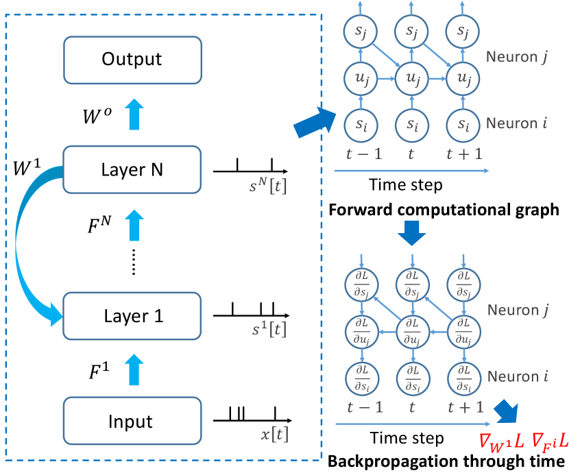
Different from ANNs, however, directly supervised training of SNNs is a hard problem due to the complex spiking neuron model which is discontinuous. To handle this problem, converting ANNs to SNNs [Hunsberger & Eliasmith, 2015, Rueckauer et al., 2017, Sengupta et al., 2019, Rathi et al., 2020, Deng & Gu, 2021, Yan et al., 2021], or many direct SNN training methods [Wu et al., 2018, Bellec et al., 2018, Jin et al., 2018, Shrestha & Orchard, 2018, Wu et al., 2019, Neftci et al., 2019, Zhang & Li, 2019, Kim et al., 2020a, Zheng et al., 2021, Bohte et al., 2002, Zhang & Li, 2020, Kim et al., 2020a, Xiao et al., 2021, Meng et al., 2022a] have been proposed to incorporate deep learning into SNNs [Tavanaei et al., 2019]. While these methods can partly solve the problems of unsatisfactory performance or high latency, they require complex computation for gradient calculation or approximation rather than the same spike-based computation as the inference process. They aim at training SNNs with general computational operations and deploying trained models for energy-efficient inference with spiking operations.
As a different direction compared with these methods, it is an important problem to consider if the training process can also take advantage of the spiking nature of common spiking neurons so that the computation of inference and training is consistent and the training process can also share the energy efficiency with event-driven computation. The consistency of the inference and training computation may also pave a path for directly training SNNs on neuromorphic hardware instead of training models on commonly used computational units and deploying them on chips. A few previous works try to train SNNs with spikes [Guerguiev et al., 2017, Neftci et al., 2017, Samadi et al., 2017, O’Connor & Welling, 2016, Thiele et al., 2019, 2020]. They either are based on direct feedback alignment (DFA) [Nøkland, 2016] and perform poorly, or require special neuron models [Thiele et al., 2019, 2020] that are hardly supported. Besides, they only focus on feedforward network structures imitated from ANNs, which ignores feedback connections that are ubiquitous in the human brain and enable neural networks to be shallower and more efficient [Kubilius et al., 2019, Xiao et al., 2021]. Actually, feedback structures suit SNNs more since SNNs will naturally compute with multiple time steps, which can reuse representations and avoid additional uneconomical costs to unfold along the time as in ANNs [Xiao et al., 2021, Kim et al., 2022]. So training algorithms for feedback SNNs, which may also be degraded for feedforward structures by taking feedback as zero, is worth more exploration.
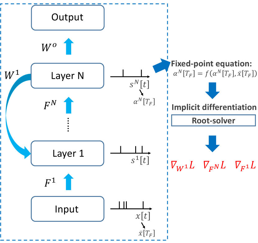
An ideal SNN training method should tackle the common problems, be suitable for flexible structures (feedforward or feedback), and be with spike-based computation for efficiency and high neuromorphic plausibility. The implicit differentiation on the equilibrium state (IDE) method [Xiao et al., 2021], which is recently proposed to train feedback spiking neural networks (FSNNs), is a promising method that may be generalized to spike-based learning for the requirement. They derive that the forward computation of FSNNs converges to an equilibrium state, which follows a fixed-point equation. Based on it, they propose to train FSNNs by implicit differentiation on this equation, which tackles the common difficulties for SNN training including non-differentiability and large memory costs, and has interesting local update properties. In their method, however, they leverage general root-finding methods rather than spike-based computation to solve implicit differentiation.
In this work, we extend the IDE method to spike-based IDE (SPIDE), which fulfills our requirements and has great potential for energy-efficient training with spike-based computation. We introduce ternary spiking neuron couples and propose to solve implicit differentiation by spikes based on them. Our method is also applicable to feedforward structures by setting the feedback connection as zero. In practice, however, it may require long time steps to stabilize the training with spikes due to the approximation error for gradients. So we further dive into the approximation error from the statistical perspective and propose to simply adjust the reset potential of SNNs to achieve an unbiased estimation of gradients and reduce the estimation variance of SNN computation. With these methods, we can train our models in a small number of time steps, which can further improve the energy efficiency as well as the latency. This demonstrates the strong power of spike-based computation for training SNNs. Our contributions include:
-
1.
We propose the SPIDE method which is the first to train high-performance SNNs by spike-based computation with common neuron models. Specifically, we propose ternary spiking neuron couples and prove that implicit differentiation for gradient calculation can be solved by spikes based on this design. Our method is applicable to both feedback and feedforward structures.
-
2.
We theoretically analyze the approximation error of solving implicit differentiation by spikes, and propose to modify the reset potential to remove the approximation bias and reduce the estimation variance, which enables training in a small number of time steps.
-
3.
Experiments show the low latency and firing sparsity during training, and the theoretical estimation of energy costs demonstrates the great potential for energy-efficient training of SNNs with spike-based computation. The performance on MNIST, CIFAR-10, CIFAR-100 and CIFAR10-DVS are competitive as well.
2 Related Work
SNN Training Methods
| Method | High Perform. | Low Latency | Struc. Flexi. | Common Neuron Model | Spike-based | Neuro. Plaus. |
|---|---|---|---|---|---|---|
| ANN-to-SNN | ✓ | ✓* | ✓ | Low | ||
| BPTT with Surrogate Gradients | ✓ | ✓ | ✓ | ✓ | Low | |
| DFA with Spikes | ? | ✓ | ✓ | High | ||
| SpikeGrad [Thiele et al., 2020] | ✓ | ? | ✓ | Medium | ||
| IDE [Xiao et al., 2021] | ✓ | ✓ | ✓ | ✓ | Low | |
| SPIDE (ours) | ✓ | ✓ | ✓ | ✓ | ✓ | High |
-
*
Typical ANN-to-SNN methods require high latency. Some recent state-of-the-art works have largely improved this.
Early works seek biologically inspired methods to train SNNs, e.g. spike-time dependent plasticity (STDP) [Diehl & Cook, 2015, Kheradpisheh et al., 2018] or reward-modulated STDP [Legenstein et al., 2008]. Since the rise of successful ANNs, several works try to convert trained ANNs to SNNs to obtain high performance [Hunsberger & Eliasmith, 2015, Rueckauer et al., 2017, Sengupta et al., 2019, Rathi et al., 2020, Deng & Gu, 2021, Yan et al., 2021, Li et al., 2021a, Stöckl & Maass, 2021]. However, they typically suffer from extremely large time steps (some recent state-of-the-art works largely improved this [Li et al., 2021a, Bu et al., 2022, Meng et al., 2022b]) and their structures are limited in the scope of ANNs. Others try to directly train SNNs by backpropagation through time (BPTT) and use surrogate derivative for discontinuous spiking functions [Lee et al., 2016, Wu et al., 2018, Bellec et al., 2018, Jin et al., 2018, Shrestha & Orchard, 2018, Wu et al., 2019, Zhang & Li, 2019, Neftci et al., 2019, Zheng et al., 2021, Fang et al., 2021b, Li et al., 2021b, Fang et al., 2021a, Deng et al., 2022] or compute gradient with respect to spiking times [Bohte et al., 2002, Zhang & Li, 2020, Kim et al., 2020a]. However, they suffer from approximation errors and large training memory costs, and their optimization with surrogate gradients is not well guaranteed theoretically. Xiao et al. [2021] propose the IDE method to train feedback spiking neural networks, which decouples the forward and backward procedures and avoids the common SNN training problems. Tandem learning [Wu et al., 2021b], ASF [Wu et al., 2021a], and DSR [Meng et al., 2022a] also share a similar thought of calculating gradients through spike rates, with the main focus only on feedforward networks with closed-form transformations between successive layers instead of implicit fixed-point equations at equilibrium states. However, all these methods require complex computation during training rather than spike-based operations. A few works focusing on training SNNs with spikes either are based on feedback alignment and limited in simple datasets [Guerguiev et al., 2017, Neftci et al., 2017, Samadi et al., 2017, O’Connor & Welling, 2016], or require special neuron models that require consideration of accumulated spikes for spike generation [Thiele et al., 2019, 2020], which is hardly supported in practice. And they are only applicable to feedforward architectures. Instead, we are the first to leverage spikes with common neuron models to train high-performance SNNs with feedback or feedforward structures. The comparison of different methods is illustrated in Table 1.
Equilibrium of Neural Networks
The equilibrium of neural networks is first considered by energy-based models, e.g. Hopfield Network [Hopfield, 1982, 1984], which view the dynamics of feedback neural networks as minimizing an energy function towards an equilibrium of the local minimum of the energy. With the energy function, recurrent backpropagation [Almeida, 1987, Pineda, 1987] and more recent equilibrium propagation (EP) [Scellier & Bengio, 2017] are proposed to train neural networks. These methods rely on the definition of the energy function and are hardly competitive with deep neural networks. With the steady state of equilibrium, the contrastive Hebbian learning method [Xie & Seung, 2003] is also proposed to train neural networks, which is composed of a two-phase anti-Hebbian and Hebbian procedure and is shown equivalent to backpropagation in the limit of weak feedback. Detorakis et al. [2019] propose a variant of this method with random feedback weights which is similar to feedback alignment. However, these methods hardly reach the high performance of backpropagation. Recently, a new branch of deep equilibrium models [Bai et al., 2019, 2020] is proposed. They interpret the computation of weight-tied deep ANNs as solving a fixed-point equilibrium point, and correspondingly propose implicit models which are defined by solving the equilibrium equations and trained by solving implicit differentiation. Their equilibrium is defined by fixed-point equations rather than energy functions and they can achieve superior performance. These works focus on ANNs rather than SNNs, except that Mesnard et al. [2016], O’Connor et al. [2019] and Martin et al. [2021] generalize the idea of EP to SNNs. They follow the energy-based EP method to approximate the gradients, which is different from the equilibrium and the training method in this work, and they are limited to tiny network scales and simple datasets. As for the equilibrium of SNNs, Zhang et al. [2018a, b] consider the equilibrium state of the membrane potential as an unsupervised learning part, Li & Pehlevan [2020] and Mancoo et al. [2020] consider the equilibrium from the perspective of solving constrained optimization problems, and Xiao et al. [2021] draw inspiration from deep equilibrium models to view feedback SNNs as evolving along time to an equilibrium state following a fixed-point equation and propose to train FSNNs by implicit differentiation on the equilibrium state (IDE). These methods do not consider training SNNs with spike-based computation. Differently, this work extends IDE to spike-based IDE, which extends the thought of equilibrium of spikes to solving implicit differentiation and enables the whole training procedure to be based on spike computation with common neuron models, providing the potential for energy-efficient training of SNNs.
3 Preliminaries
We first introduce preliminaries about spiking neural network models and the IDE training method [Xiao et al., 2021].
3.1 Spiking Neural Network Models
Spiking neurons draw inspiration from the human brain to communicate with each other by spikes. Each neuron integrates information from input spike trains by maintaining a membrane potential through a differential equation and generates an output spike once the membrane potential exceeds a threshold, following which the membrane potential is reset to the reset potential. We consider the commonly used integrate and fire (IF) and leaky integrate and fire (LIF) neuron models, whose general discretized computational form is:
| (1) |
where is the membrane potential of neuron at time step , is the binary output spike train of neuron , is the connection weight from neuron to neuron , is bias, is the Heaviside step function, is the firing threshold, is the reset potential, and for the IF model while is a leaky term for the LIF model. We use subtraction as the reset operation. is usually taken as in previous work, while we will reconsider it in Section 4.3. We mainly consider the IF neuron model by default and will demonstrate that our method is applicable to the LIF model as well.
3.2 Background about the IDE Training Method
Due to the complex spiking neuron model which is discontinuous, directly supervised training of SNNs is a hard problem, since the explicit computation is non-differentiable and therefore backpropagation along the forward computational graph is problematic. The IDE training method [Xiao et al., 2021] considers another approach to calculate gradients that does not rely on the exact reverse of the forward computation, which avoids the problem of non-differentiability as well as large memory costs by BPTT methods with surrogate gradients. Specifically, the IDE training method first derives that the (weighted) average firing rate of FSNN computation with common neuron models would gradually evolve to an equilibrium state along time, which follows a fixed-point equation. Then by viewing the forward computation of FSNN as a black-box solver for this equation, and applying implicit differentiation on the equation, gradients can be calculated only based on this equation and the (weighted) average firing rate during the forward computation rather than the exact forward procedure. Therefore, the forward and backward procedures are decoupled and the non-differentiability is avoided.
We briefly introduce the conclusion of equilibrium states in Section 3.2.1 and the IDE method in Section 3.2.2.
3.2.1 Equilibrium States of FSNNs
Xiao et al. [2021] derive that the (weighted) average rate of spikes during FSNN computation with common neuron models would converge to an equilibrium state following a fixed-point equation given convergent inputs. We first focus on the conclusions with the discrete IF model under both single-layer and multi-layer feedback structures. The single-layer structure has one hidden layer of neurons with feedback connections on this layer. The update equation of membrane potentials after reset is (let ):
| (2) |
where and are the vectors of membrane potentials and spikes of these neurons, is the input at time step , is the feedback weight matrix, and is the weight matrix from inputs to these neurons. The average input and average firing rate are defined as and , respectively. Define .
The equilibrium state of the single-layer FSNN is described as [Xiao et al., 2021]: If the average inputs converge to an equilibrium point , and there exists such that , then the average firing rates of FSNN with discrete IF model will converge to an equilibrium point , which satisfies the fixed-point equation . Note that they take in this conclusion, if we consider nonzero , the constraint and the fixed-point equation should be and .
The multi-layer structure incorporates more non-linearity into the equilibrium fixed-point equation, which has multiple layers with feedback connections from the last layer to the first layer. The update equations of membrane potentials after reset are expressed as:
| (3) |
The equilibrium state of the multi-layer FSNN with is described as [Xiao et al., 2021]: If the average inputs converge to an equilibrium point , and there exists such that , then the average firing rates of multi-layer FSNN with discrete IF model will converge to equilibrium points , which satisfy the fixed-point equations and , where and .
As for the LIF model, the weighted average firing rate will be considered to represent information: the weighted average input and weighted average firing rate are defined as and , respectively. Xiao et al. [2021] has derived the equilibrium states of FSNN under the LIF model as well. The conclusions are similar to the IF model and the equilibrium states follow the same fixed-point equation, except that weighted average firing rates (inputs) are considered and there would be bounded random error for the equilibrium state. We can view it as an approximate solver for the equilibrium state.
3.2.2 IDE Training Method
Based on the equilibrium states in Section 3.2.1, we can train FSNNs by calculating gradients with implicit differentiation [Xiao et al., 2021]. Let denote the fixed-point equation of the equilibrium state which is parameterized by , , and let denote the objective function with respect to the equilibrium state . The implicit differentiation satisfies [Bai et al., 2019] (we follow the numerator layout convention for derivatives). Therefore, the differentiation of for parameters can be calculated based on implicit differentiation as:
| (4) |
where is the inverse Jacobian of evaluated at . The calculation of inverse Jacobian can be avoided by solving an alternative linear system [Bai et al., 2019, 2020, Xiao et al., 2021]:
| (5) |
Note that a readout layer after the last layer of neurons will be constructed for output [Xiao et al., 2021], which is composed of neurons that will not spike and will do classification based on accumulated membrane potentials (e.g. realized by a very large threshold). Then the output is equivalent to a linear transformation on the approximate equilibrium state, i.e. , and the loss will be calculated between and labels with a common criterion such as cross-entropy. Then the gradient on the equilibrium state can be calculated. For the solution of implicit differentiation, Xiao et al. [2021] follow Bai et al. [2019, 2020] to leverage root-finding methods, while we will solve it by spike-based computation, as will be derived in Section 4. We consider that the (weighted) average firing rates during the forward computation of FSNNs at time step roughly reach the equilibrium state. Then by substituting by in the above equations, gradients for the parameters can be calculated only with and the equation, and we calculate them based on spikes. With the gradients, first-order optimization methods such as SGD [Rumelhart et al., 1986] and its variants can be applied to update parameters.
4 Spike-based Implicit Differentiation on the Equilibrium State
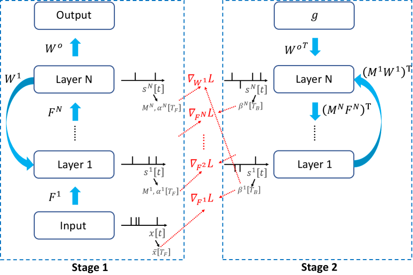
In this section, we present our SPIDE method that calculates the whole training procedure based on spikes. We first introduce ternary spiking neuron couples in Section 4.1 and how to solve implicit differentiation in Section 4.2. Then we theoretically analyze the approximation error and propose the improvement in Section 4.3. Finally, a summary of the training pipeline is presented in Section 4.4. We also provide a brief illustration figure of the overall process in Figure 1.
4.1 Ternary Spiking Neuron Couples
The common spiking neuron model only generates spikes when the membrane potential exceeds a positive threshold, which limits the firing rate from representing negative information. To enable approximation of possible negative values for implicit differentiation calculation in Section 4.2, we require negative spikes, whose expression could be:
| (6) |
and the reset is the same as usual: . Direct realization of such ternary output, however, may be not supported by common neuromorphic computation of SNNs.
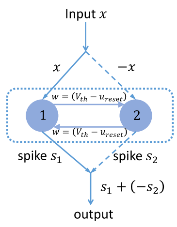
We propose to leverage two coupled common neurons to realize this computation. As illustrated in Figure 2, the two coupled neurons with the common IF model (Eq. (1)) receive opposite inputs and output opposite spikes, which aim to deal with positive information and negative information with spikes, respectively. They should share a reset operation in order to accord with Eq. (6), which can be realized by the connections between them: as we use subtraction as the reset operation, the connection whose weight equals enables one neuron to reset the other equivalently. To see how this works, consider the condition that the accumulated membrane potential of neuron 1 reaches , then neuron 1 would generate a spike and reset, and the output is this positive spike. At the same time, the membrane potential of neuron 2 is and the neuron will not fire and reset, but the spike from neuron 1 will reset it to , which accords with our desired reset for ternary output. Similarly, if the inputs are negative, neuron 2 will generate a spike which will be treated negative as output, and both neurons are reset. For the operation of taking negative, one solution is to enable the reverse operation on hardware; another is to reconnect neuron 2 with other neurons while taking the weight negative to that of neuron 1. As for most existing neuromorphic hardware, the double connections to the two coupled neurons are more feasible, and this implies that twice the synaptic operations are needed for each spike. Therefore, such kind of coupled common neurons can realize ternary output.
We note that the SpikeGrad algorithm [Thiele et al., 2020] also requires neurons for ternary output. However, they do not consider how such kind of operation can be implemented with the common neuron models that follow the basic properties of biological neurons, and moreover, they propose another modified neuron model in practice that requires consideration of accumulated spikes for spike generation, which is hardly supported in practice. Differently, our method is with the common neuron model (IF or LIF). This can be suitable for neuromorphic hardware. Also, SpikingYOLO [Kim et al., 2020b] proposes ternary neurons for the inference of SNNs converted from ANNs without considering the implementation by the common neuron models. Our ternary spiking neuron couples may also provide a way to implement their method on hardware.
4.2 Solving Implicit Differentiation with Spikes
Based on the coupled neurons in Section 4.1, we can solve implicit differentiation with spikes. For notation simplicity, we directly use Eq. (6) as a ternary neuron without detailing coupled neurons below. Our main focus is on solving Eq. (5) with spikes. We first consider the IF neuron model by default and will include the LIF model later. The brief outline for the derivation is: we first derive the update equation of membrane potentials, then we derive the equivalent equation of the rate of spikes with eliminating perturbation, and finally, we prove that the firing rate converges to the solution of Eq. (5).
We first consider the single-layer condition. Let denote the average firing rate of these neurons after the forward computation with time steps as an approximate equilibrium state (we treat the forward procedure as the first stage), denote the gradient of the loss function on this approximate equilibrium state, and denote a mask indicator based on the firing condition in the first stage, where . We will have another time steps in the second backward stage to calculate implicit differentiation. We set the input to these neurons as at all time steps, which can be viewed as input currents [Zhang & Li, 2020, Xiao et al., 2021]. Then along the inverse connections of neurons and with a mask on neurons or weights and an output rescale, the computation of FSNN with ternary neurons is:
| (7) |
where and are the threshold and reset potential during the first and second stage, respectively. Define the ‘average firing rate’ at this second stage as , and , then through summation, we have (let ):
| (8) |
Since there would be at most spikes during time steps, should be bounded in the range of . The membrane potential will maintain the exceeded terms, i.e. define , we can divide as , where is the exceeded term while is a bounded term [Xiao et al., 2021] which is typically bounded in the range of . Then, Eq. (8) turns into:
| (9) |
where . Note that if and are in an appropriate range, there would be no exceeded term and will not take effect. Indeed we will rescale the loss to control the range of , as will be indicated in Section 4.3. With this consideration, we can prove that converges to the solution of Eq. (5).
Theorem 1.
If there exists such that , then the average firing rate will converge to an equilibrium point . When , and there exists such that and , then is the solution of Eq. (5).
The proof and discussion of assumptions are in A. With Theorem 1, we can solve Eq. (5) by simulating this second stage of SNN computation to obtain the ‘firing rate’ as the approximate solution. Plugging this solution to Eq. (4), the gradients can be calculated by: and
.
Note that in practice, even if the data distribution is not in a proper range, we can still view as a kind of clipping for improperly large numbers, which is similar to empirical techniques like “gradient clipping” to stabilize the training.
Then we consider the extension to the multi-layer condition. Let denote the average firing rate of neurons in layer after the forward computation, denote the gradient of the loss function on the approximate equilibrium state of the last layer, and denote the mask indicators. Similarly, we will have another time steps in the second stage and set the input to the last layer as at all time steps. The computation of FSNN with ternary neurons is calculated as:
| (10) |
The ‘average firing rates’ are similarly defined for each layer, and the equivalent form can be similarly derived as:
| (11) |
The convergence of the ‘firing rate’ at the last layer to the solution of Eq. (5) can be similarly derived as Theorem 1. However, we need to calculate gradients for each parameter as Eq. (4), which is more complex than the single-layer condition. Actually, we can derive that the ‘firing rates’ at each layer converge to equilibrium points, based on which the gradients can be easily calculated with information from the adjacent layers. Theorem 2 gives a formal description.
Theorem 2.
If there exists such that , then the average firing rates will converge to equilibrium points . When , and there exists such that and , then is the solution of Eq. (5), and , where .
The functions are defined in Section 3.2.1. For the proof please refer to B. With Theorem 2, by putting the solutions into Eq. (4), the gradients can be calculated by: , , , and .
Note that the gradient calculation shares an interesting local property, i.e. it is proportional to the firing rates of the two neurons connected by it: . During calculation, since we will have the firing rate of the first stage before the second stage, this calculation can also be carried out by event-based calculation triggered by the spikes in the second stage. So the weight update could be event-driven as well.
Also, note that the theorems still hold if we degrade our feedback models to feedforward ones by setting feedback connections as zero. In this setting, the dynamics and equilibriums degrade to direct functional mappings, and the implicit differentiation degrades to the explicit gradient. We can still approximate gradients with this computation.
In the following, we take by default to fulfill the assumption of theorems (it may take other values if we correspondingly rescale the outputs and we set for simplicity). Other techniques like dropout can also be included. Please refer to C for details.
SPIDE with LIF neuron model
The above conclusions show that we can leverage the equilibrium states with the IF neuron model to solve implicit differentiation with spikes. As introduced in Section 3.2.1, we can also derive the equilibrium states with the LIF neuron model by considering the weighted average firing rate, and the equilibrium fixed-point equations would have the same form as those of the IF model except for some bounded random error. Therefore, with the same thought, our SPIDE method can leverage LIF neurons to approximate the solution of implicit differentiation as well. We can replace IF neurons and average firing rates with LIF neurons and weighted average firing rates, and it will gradually approximate the same equilibrium states as in Theorem 1 and Theorem 2 with bounded random error. The derivation is similar to Xiao et al. [2021] and Theorems, and the repetitive details are omitted here.
4.3 Reducing Approximation Error
Section 4.2 derives that we can solve implicit differentiation with spikes, as the average firing rate will gradually converge to the solution. In practice, however, we will simulate SNNs for finite time steps, and a smaller number of time steps is better for lower energy consumption. This will introduce approximation error which may hamper training. In this subsection, we theoretically study the approximation error and propose to adjust the reset potential to reduce it. Inspired by the theoretical analysis on quantized gradients [Chen et al., 2020], we will analyze the error from the statistical perspective.
For the ‘average firing rates’ in Eq. (8) and the multilayer counterparts, the approximation error to the equilibrium states consists of three independent parts , and : the first is that is the exceeded term due to the limitation of spike number, the second is which can be viewed as a bounded random variable, and the third is the convergence error of the iterative update scheme without , i.e. let denote the iterative sequences for solving as , the convergence error is . The second part can be again decomposed into two independent components : is the quantization effect due to the precision of firing rates ( for time steps) if we first assume the same average inputs at all time steps, and is due to the random arrival of spikes rather than the average condition, as there might be unexpected output spikes, e.g. the average input is and the expected output should be , but two large positive inputs followed by one larger negative input at the last time would generate two positive spikes while only one negative spike. So the error is divided into: . Since the iterative formulation is certain for , we focus on , and .
Firstly, the error due to the quantization effect is influenced by the input scale and time steps . To enable proper input scale and smaller time steps, we rescale the loss function by a factor , since the magnitude of gradients with cross-entropy loss is relatively small. We scale the loss to an appropriate range so that information can be propagated by SNNs in smaller time steps, and most signals are in the range of as analyzed in Section 4.2. The base learning rate is scaled by correspondingly. This is also adopted by Thiele et al. [2020].
Then given the scale and number of time steps, , and can be treated as random variables from statistical perspective, and we view as stochastic estimators for the equilibrium states with . For the stochastic optimization algorithms, the expectation and variance of the gradients are important for convergence and convergence rate [Bottou, 2010], i.e. we hope an unbiased estimation of gradients and smaller estimation variance. As for and , they depends on the input data and the expectations are (the positive and negative parts have the same probability). While for , it will depend on our hyperparameters and . Since the remaining terms in caused by the quantization effect is in the range of for positive terms while for negative ones, given and considering the uniform distribution, only when , for both positive and negative terms. Therefore, we should adjust the reset potential from commonly used 0 to for unbiased estimation, as described in Proposition 3.
Proposition 3.
For fixed and uniformly distributed inputs and , only when , are unbiased estimators for .
Also, taking achieves the smallest estimation variance for the quantization effect , considering the uniform distribution on . Since the effects of , and are independent of and their variance is certain given inputs, it leads to Proposition 4.
Proposition 4.
Taking reduces the variance of estimators .
With this analysis, we will take in the following. For and during the first forward stage, we will also take .
4.4 Details and Training Pipeline
The original IDE method [Xiao et al., 2021] leverages other training techniques including modified batch normalization (BN) and restriction on weight spectral norm. Since the batch statistical information might be hard to obtain for calculation of biological systems and neuromorphic hardware, and training with the BN operation is hard to be implemented by spike-based calculation, we drop BN in our SPIDE method. The restriction on the weight norm, however, is necessary for the convergence of feedback models, as indicated in theorems. We will adjust it for a more friendly calculation, please refer to C for details.
Input:
Network parameters ; Time steps ; Forward threshold ; Dropout rate ; Input data ;
Output:
Output of the readout layer .
Input:
Network parameters ; Forward output ; Label ; Time steps ; Forward threshold ; Backward threshold ; Other hyperparameters and saved variables;
Output:
Trained network parameters .
We summarize our training pipeline as follows. There are two stages for the forward and backward procedures respectively. In the first stage, SNNs receive inputs and perform the calculation as Eq. (1,2,3) for time steps, after which we get the output from the readout layer, and save the average inputs as well as the average firing rates and masks of each layer for the second stage. In the second stage, the last layer of SNNs will receive gradients for outputs and perform calculation along the inverse connections as Eq. (6,7,10) for time steps, after which we get the ‘average firing rates’ of each layer. With firing rates from two stages, the gradients for parameters can be calculated as in Section 4.2 and then the first-order optimization algorithm is applied to update the parameters. We provide detailed pseudocodes for both stages in Algorithm 1 and Algorithm 2, respectively. Figure 1 also illustrates the overall process.
5 Experiments
In this section, we conduct experiments to demonstrate the effectiveness of our method and the great potential for energy-efficient training. We simulate the computation on common computational units. Please refer to C for implementation details and descriptions.
| MeanStd (Best) | |
|---|---|
| 50 | 88.41%0.48% (89.07%) |
| 100 | 89.17%0.14% (89.35%) |
| 250 | 89.61%0.11% (89.70%) |
| 500 | 89.57%0.08% (89.67%) |
Effectiveness with a small number of backward time steps
As shown in Table 5, we can train high-performance models with low latency () in a small number of backward time steps during training (e.g. ), which indicates the low latency and high energy efficiency. Note that conventional ANN-SNN methods require hundreds to thousands of time steps just for satisfactory inference performance, and recent progress of the conversion methods and direct training methods show that relatively small time steps are enough for inference, while we are the first to demonstrate that even training of SNNs can be carried out with spikes in a very small number of time steps. This is due to our analysis and improvement to reduce the approximation error, as illustrated in the following ablation study.
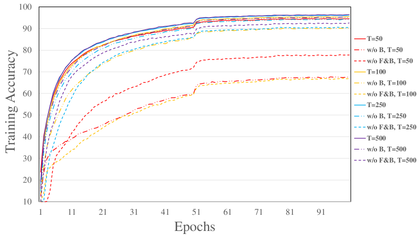
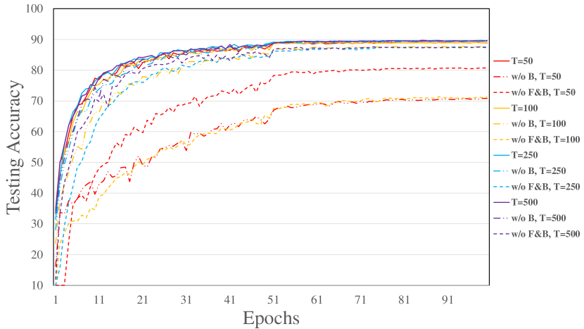
Ablation study of reducing the approximation error
We conduct ablation study on our improvement to reduce the approximation error by setting the reset potential as negative threshold. To formulate equivalent equilibrium states, we take the same and the same , and we consider the following settings: (1) both forward and backward stages apply our improvement, i.e. ; (2) remove the improvement on the backward stage, i.e. ; (3) remove the improvement on both forward and backward stages, i.e. and . The latter two setting are denoted by “w/o B” and “w/o F&B” respectively. The models are trained on CIFAR-10 with AlexNet-F structure and 30 forward time steps. The training and testing curves under different settings and backward time steps are illustrated in Figure 3. It demonstrates that without our improvement, the training can not perform well within a small number of backward time steps, probably due to the bias and large variance of the estimated gradients. When the backward time steps are large, the performance gap is reduced since the bias of estimation is reduced. It shows the superiority of our improvement in training SNNs within a small number of backward time steps.
Firing rate statistics and potential of energy efficiency
| Method | OpNum | OpEnergy | Cost |
|---|---|---|---|
| SPIDE (ours) | (FiringRate ) | 0.9 (AC) | |
| STBP | 30 () | 4.6 (MAC) |
| Method | OpNum | OpEnergy | Cost |
|---|---|---|---|
| Spike-based | (FiringRate ) | 0.9 (AC) | |
| Not spike-based | 30 () | 4.6 (MAC) |
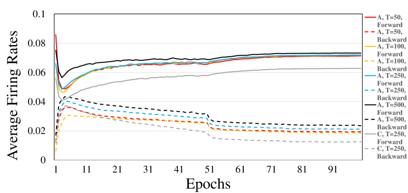
Since the energy consumption of event-driven SNNs is proportional to the number of spikes, we present the average firing rates for forward and backward stages (for backward, both positive and negative spikes are considered as firing) in Figure 5. It shows the firing sparsity of our method, and spikes are sparser in the backward stage with around only . Combined with the small number of time steps, this demonstrates the great potential for the energy-efficient training of SNNs with spike-based computation. We theoretically estimate and compare the energy costs for the operations of neurons of our method and the representative STBP method111The energy costs of the IDE method are hard to estimate because IDE leverages root-finding methods (e.g. Broyden’s method) to solve implicit differentiation, which may involve many complex operations and the iteration number may depend on the convergence speed. If we consider the fixed-point update scheme with a fixed iteration number as the root-finding method in the IDE, its operation number is about the same as STBP with time steps to backpropagate. As the iteration threshold of IDE is usually taken as 30 (i.e. the maximum iteration number for root-finding methods if the update does not converge before it), the energy estimation of STBP with 30 time steps can also be an effective surrogate result for IDE.. We mainly focus on the energy of the backward stage which is made spike-based and only requires accumulation (AC) operations by SPIDE while requiring multiply and accumulate (MAC) operations by STBP. Our operation number is estimated as the firing rate multiplied by backward time steps , and that of STBP is the forward time steps as STBP will repeat the computation for times to backpropagate through time. According to the 45nm CMOS processor, the energy for 32bit FP MAC operation is 4.6 pJ, and for AC operation is 0.9 pJ. Therefore, as shown in Table 5, when , our method could achieve approximately reduction in energy cost222Note that the realization of ternary spiking neuron couples may require twice the synaptic operations under some cases (see Section 4.1), so the energy cost reduction may be halved. Despite this, we could still achieve approximately reduction in energy cost.. Additionally, if we consider that the forward computation of STBP also has to be simulated by, e.g. GPU, to be compatible with the backward stage and the computation is not spike-based, while ours may be deployed with neuromorphic hardware for spike-based computation, then the forward stage during training can also reduce the energy by around , as shown in Table 5. Note that even for STBP with fewer forward time steps, e.g. 12 or 6, the energy costs of SPIDE for the backward stage are still about or less than STBP, and our result in Table 6 will show that SPIDE is also effective with smaller .
| MNIST | ||||||
|---|---|---|---|---|---|---|
| Method | Network structure | MeanStd (Best) | Neurons | Params | ||
| BP [Lee et al., 2016] | 20C5-P2-50C5-P2-200 | 200 | N.A. | (99.31%) | 33K | 518K |
| STBP [Wu et al., 2018] | 15C5-P2-40C5-P2-300 | 30 | N.A. | (99.42%) | 26K | 607K |
| IDE [Xiao et al., 2021] | 64C5 (F64C5) | 30 | N.A. | 99.53%0.04% (99.59%) | 13K | 229K |
| SpikeGrad [Thiele et al., 2020] | 15C5-P2-40C5-P2-300 | Unknown | Unknown | 99.38%0.06% (99.52%) | 26K | 607K |
| SPIDE (ours) | 64C5s-64C5s-64C5 (F64C3u) | 30 | 100 | 99.34%0.02% (99.37%) | 20K | 275K |
| SPIDE (ours, degraded) | 15C5-P2-40C5-P2-300 | 30 | 100 | 99.44%0.02% (99.47%) | 26K | 607K |
| CIFAR-10 | ||||||
|---|---|---|---|---|---|---|
| Method | Network structure | MeanStd (Best) | Neurons | Params | ||
| ANN-SNN Sengupta et al. [2019] | VGG-16 | 2500 | N.A. | (91.55%) | 311K | 15M |
| ANN-SNN [Deng & Gu, 2021] | CIFARNet | 400-600 | N.A. | (90.61%) | 726K | 45M |
| STBP [Wu et al., 2019] | AlexNet | 12 | N.A. | (85.24%) | 595K | 21M |
| STBP (w/o NeuNorm) [Wu et al., 2019] | CIFARNet | 12 | N.A. | (89.83%) | 726K | 45M |
| STBP [Xiao et al., 2021] | AlexNet-F | 30 | N.A. | (87.18%) | 159K | 3.7M |
| IDE [Xiao et al., 2021] | AlexNet-F | 30 | N.A. | 91.74%0.09% (91.92%) | 159K | 3.7M |
| IDE [Xiao et al., 2021] | CIFARNet-F | 30 | N.A. | 92.08%0.14% (92.23%) | 232K | 11.8M |
| SpikeGrad [Thiele et al., 2020] | CIFARNet | Unknown | Unknown | 89.49%0.28% (89.99%) | 726K | 45M |
| SPIDE (ours) | AlexNet-F | 12 | 250 | 89.11%0.29% (89.43%) | 159K | 3.7M |
| SPIDE (ours) | AlexNet-F | 30 | 250 | 89.61%0.11% (89.70%) | 159K | 3.7M |
| SPIDE (ours) | CIFARNet-F | 30 | 250 | 89.94%0.17% (90.13%) | 232K | 11.8M |
Competitive performance on common datasets
We evaluate the performance of our method on static datasets MNIST [LeCun et al., 1998], CIFAR-10, and CIFAR-100 [Krizhevsky & Hinton, 2009], as well as the neuromorphic dataset CIFAR10-DVS [Li et al., 2017]. We compare our method to several ANN-SNN methods [Sengupta et al., 2019, Deng & Gu, 2021], direct SNN training methods [Wu et al., 2018, Xiao et al., 2021], and SpikeGrad [Thiele et al., 2020] with similar network structures. As shown in Table 5 and Table 6, we can train both feedforward and feedback SNN models with a small number of time steps and our trained models achieve competitive results on MNIST and CIFAR-10. Compared with SpikeGrad [Thiele et al., 2020], we can use fewer neurons and parameters due to flexible network structure choices, and a small number of time steps while they do not report this important feature. Besides, we use common neuron models while they require special neuron models that are hardly supported, as indicated in Section 4.1.
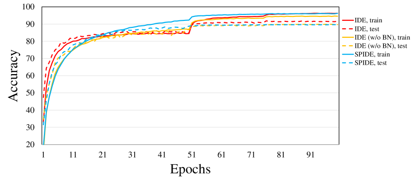
Compared with the original IDE method [Xiao et al., 2021], our generalization performance is poorer as we discard the BN component. As shown in Figure 5, the SPIDE method can achieve the same training accuracy as the IDE method, while the generalization performance is poorer. Since the hyperparameters are the same for experiments, except that we drop the modified BN component (as explained in Section 4.4), the performance gap may be caused by the implicit regularization effect of BN. We try to drop the modified BN component for IDE and the results in Figure 5 show that it achieves similar performance (89.93%) as SPIDE. Therefore, the optimization ability of the SPIDE method should be similar to that of IDE, while future work could investigate techniques that are similar to BN but more friendly to the spike-based computation of SNNs to further improve the performance.
| Method | Network structure | BN | MeanStd (Best) | Neurons | Params | ||
|---|---|---|---|---|---|---|---|
| BP [Thiele et al., 2020] | CIFARNet | Unknown | N.A. | (64.69%) | 726K | 45M | |
| IDE [Xiao et al., 2021] | CIFARNet-F | ✓ | 30 | N.A | 71.56%0.31% (72.10%) | 232K | 14.8M |
| SpikeGrad [Thiele et al., 2020] | CIFARNet | Unknown | Unknown | (64.40%) | 726K | 45M | |
| SPIDE (ours) | CIFARNet-F | 30 | 100 | 63.57%0.30%(63.91%) | 232K | 14.8M | |
| SPIDE (ours) | CIFARNet-F | 30 | 250 | 64.00%0.11%(64.07%) | 232K | 14.8M |
| Method | Model | Accuracy | ||
|---|---|---|---|---|
| Gabor-SNN [Sironi et al., 2018] | Gabor-SNN | N.A | N.A | 24.5% |
| HATS [Sironi et al., 2018] | HATS | N.A | N.A | 52.4% |
| STBP [Wu et al., 2019] | Spiking CNN (LIF, w/o NeuNorm) | 40 | N.A | 58.1% |
| STBP [Wu et al., 2019] | Spiking CNN (LIF, w/ NeuNorm) | 40 | N.A | 60.5% |
| Tandem Learning [Wu et al., 2021b] | Spiking CNN (IF) | 20 | N.A | 58.65% |
| ASF-BP [Wu et al., 2021a] | Spiking CNN (IF) | Unknown | N.A | 62.5% |
| SPIDE (ours) | Spiking CNN (IF) | 30 | 250 | 60.7% |
The results on CIFAR-100 are shown in Table 7 and our model can achieve 64.07% accuracy. Compared with IDE, the performance is poorer, and the main reason is probably again the absence of BN which could be important for alleviating overfitting on CIFAR-100 with a relatively small number of images per class. The training accuracy of SPIDE is similar to IDE (around 93% v.s. around 94%) while the generalization performance is poorer. Despite this, the performance of our model is competitive for networks without BN and our model is with fewer neurons and parameters and a small number of time steps. Compared with SpikeGrad [Thiele et al., 2020], we can use fewer neurons and parameters due to flexible network structure choices, and we leverage common neuron models while they do not. Future work could investigate more suitable structures and more friendly techniques to further improve the performance.
The results on CIFAR10-DVS are shown in Table 8, and our model can achieve 60.7% accuracy. It is competitive among results of common SNN models, demonstrating the effectiveness of our method.
The above results show the effectiveness of our method even with the constraint of purely spike-based training. We note that there are some recent works that achieve higher state-of-the-art performance [Zheng et al., 2021, Fang et al., 2021b, Li et al., 2021b, Fang et al., 2021a, Deng et al., 2022]. However, their target is different from ours which aims at training SNNs with purely spike-based computation as introduced in Section 1, and they leverage many other techniques such as batch normalization along the temporal dimension or learnable membrane time constant. We do not aim at outperforming the state-of-the-art results but demonstrate that a competitive performance can be achieved even with our constraints of purely spike-based training with common neuron models. And our future work could seek techniques friendly to neuromorphic computation to further improve the performance.
As a preliminary attempt, we provide the result of applying the scaled weight standardization (sWS) technique which is shown as a powerful method to replace BN in ResNets [Brock et al., 2021a, b] and SNNs [Xiao et al., 2022]. Particularly, sWS standardizes weights instead of activations by , where and are the mean and variance calculated along the input dimension, and the scale is determined by analyzing the signal propagation with different activation functions (typically taken as ). Brock et al. [2021a] show that normalization-free ResNets with the sWS technique can achieve a similar performance as common ResNets with BN. We apply this technique to our experiment on CIFAR-10 and the performance of the AlexNet-F structure improves from 89.61% to 90.37% and the performance of the CIFARNet-F structure improves from 89.94% to 90.85%. It shows that we can effectively leverage other techniques to improve performance.
| Dataset | Forward Model | Backward Model | MeanStd (Best) | ||
|---|---|---|---|---|---|
| MNIST | IF | IF | 30 | 100 | 99.34%0.02% (99.37%) |
| LIF | IF | 30 | 100 | 99.32%0.04% (99.37%) | |
| LIF | LIF | 30 | 100 | 99.34%0.05% (99.39%) | |
| CIFAR-10 | IF | IF | 30 | 250 | 89.94%0.17% (90.13%) |
| LIF | IF | 30 | 250 | 89.66%0.12% (89.78%) | |
| LIF | LIF | 30 | 250 | 89.54%0.14% (89.72%) | |
| CIFAR-100 | IF | IF | 30 | 250 | 64.00%0.11% (64.07%) |
| LIF | IF | 30 | 250 | 64.04%0.03% (64.06%) | |
| LIF | LIF | 30 | 250 | 63.81%0.19% (63.97%) |
Results with LIF neuron model
As introduced in Section 4.2, our SPIDE method is also applicable to the LIF neuron model. We conduct experiments on MNIST, CIFAR-10, and CIFAR-100 to verify the effectiveness of SPIDE with LIF neurons. Following [Xiao et al., 2021], the leaky term for LIF neurons is set as for MNIST and for CIFAR-10 and CIFAR-100. The network structure for CIFAR-10 and CIFAR-100 is taken as CIFARNet-F, and other details are the same as the experiment for IF neurons. The results are shown in Table 9. It demonstrates that SPIDE is also effective for LIF neurons.
6 Conclusion
In this work, we propose the SPIDE method that generalizes the IDE method to enable purely spike-based training of SNNs with common neuron models and flexible network structures. We prove that the implicit differentiation can be solved with spikes by our coupled neurons. We also analyze the approximation error due to finite time steps and propose to adjust the reset potential of SNNs. Experiments show that we can achieve competitive performance with a small number of training time steps and sparse spikes, which demonstrates the great potential of our method for energy-efficient training of SNNs with spike-based computation. As for the limitations, SPIDE and IDE mainly focus on the condition that inputs are convergent in the context of average accumulated signals, e.g. image classification with static or neuromorphic inputs. For long-term sequential data such as speech, we may define the final average inputs as the convergent inputs and directly apply our method, but the error flow throughout time is not carefully handled. An interesting future work is to generalize the methodology to time-varying inputs with more careful consideration of error flows and equilibriums, e.g. with certain time windows.
Acknowledgements
Z. Lin was supported by the major key project of PCL (No. PCL2021A12), the NSF China (No. 62276004), and Project 2020BD006 supported by PKU-Baidu Fund. Yisen Wang is partially supported by the National Natural Science Foundation of China under Grant 62006153, and Project 2020BD006 supported by PKU-Baidu Fund.
Appendix A Proof of Theorem 1
Proof.
We first prove the convergence of . Let and denote and respectively. Consider , it satisfies:
| (12) |
As , and is bounded, we have , where is a constant. Therefore is bounded. Then such that when , we have:
| (13) |
And since , we have:
| (14) |
Therefore, when , it holds that:
| (15) |
By iterating the above inequality, we have There exists such that when , , and therefore . According to Cauchy’s convergence test, the sequence converges to . Considering the limit, it satisfies .
When , and there exists such that and , the equation turns into . We have:
| (16) |
Therefore, , and we have . It means .
Taking (i.e. the fixed-point equation at the equilibrium state as in Section 3.2.1) explicitly into Eq. (5), the linear equation turns into , where are previously defined. Therefore, satisfies this equation. And since , the equation has the unique solution .
∎
Remark 1.
As for the assumptions in the theorem, firstly, when as we will take, the assumption for the convergence is weaker than that for the convergence in the forward stage (in Section 3.2.1), because as is a diagonal mask matrix. We will restrict the spectral norm of following Xiao et al. [2021] to encourage the convergence of the forward stage (in C), then this backward stage would converge as well.
The assumptions for the consistency of the solution is a sufficient condition. In practice, the weight norm will be partially restricted by weight decay and our restriction on Frobenius norm (in C), as well as the diagonal mask matrix which would be sparse if the forward firing events are sparse, and we will rescale the loss so that the input is in an appropriate range, as indicated in Section 4.3. Even if these assumptions are not satisfied, we can view as a kind of empirical clipping techniques to stabilize the training, as indicated in Section 4.2. The discussion is similar for the multi-layer condition (Theorem 2) in the next section.
Appendix B Proof of Theorem 2
Proof.
We first prove the convergence of .
Let and denote and respectively. Let
Then .
We have:
| (17) |
where ,
and .
For the term and , they are bounded by:
| (18) | ||||
and has the same form as by substituting with .
Since , we have:
| (19) | ||||
And since is bounded, then such that when , we have:
| (20) |
Then , and there exists such that when , . According to Cauchy’s convergence test, converges to , which satisfies . Considering the limit, converges to , which satisfies .
When , and there exists such that and , we have:
| (21) |
Therefore, , and , where , (i.e. is without the function ). It means and .
Taking and (i.e. the fixed-point equation at the equilibrium state as in Section 3.2.1) explicitly into Eq. (5), the linear equation turns into . Therefore, satisfies this equation. And since , the equation has the unique solution . Further, because , where , we have .
∎
Appendix C Training details
C.1 Dropout
Dropout is a commonly used technique to prevent over-fitting, and we follow Bai et al. [2019, 2020], Xiao et al. [2021] to leverage variational dropout, i.e. the dropout of each layer is the same at different time steps. Since applying dropout on the output of neurons is a linear operation with a mask and scaling factor, it can be integrated into the weight matrix without affecting the conclusions of convergence. The detailed computation with dropout is also illustrated in the pseudocode in Section 4.4.
C.2 Restriction on weight norm
As indicated in the theorems, a sufficient condition for the convergence to equilibrium states in both forward and backward stages is the restriction on the weight spectral norm. Xiao et al. [2021] leverages re-parameterization to restrict the spectral norm, i.e. they re-parameterize as , where is computed as the implementation of Spectral Normalization and is a learnable parameter to be clipped in the range of ( is a constant). However, the computation of spectral norm and re-parameterization may be unfriendly to neuromorphic computation. We adjust it for a more friendly calculation as follows.
First, the spectral norm is upper-bounded by the Frobenius norm: . We can alternatively restrict the Frobenius norm which is easier to compute. Further, considering that connection weights may not be easy for readout compared with neuron outputs, we can approximate by , according to the Hutchinson estimator [Hutchinson, 1989]. It can be viewed as source neurons outputting noises and target neurons accumulating signals to estimate the Frobenius norm. We will estimate the norm based on the Monte-Carlo estimation (we will take 64 samples), which is similarly adopted by Bai et al. [2021] to estimate the norm of their Jacobian matrix. Then based on the estimation, we will restrict as where , is a constant for norm range. This estimation and calculation may correspond to large amounts of noises in our brains, and a feedback inhibition on connection weights based on neuron outputs.
Following Xiao et al. [2021], we only restrict the norm of feedback connection weight for the multi-layer structure, which works well in practice.
C.3 Other details
Details on MNIST, CIFAR-10, and CIFAR-100
For SNN models with feedback structure, we set in the forward stage to form an equivalent equilibrium state as Xiao et al. [2021]. The constant for restriction in C.2 is . Following Xiao et al. [2021], we train models by SGD with momentum for 100 epochs. The momentum is 0.9, the batch size is 128, and the initial learning rate is 0.05. For MNIST, the learning rate is decayed by 0.1 every 30 epochs, while for CIFAR-10 and CIFAR-100, it is decayed by 0.1 at the 50th and 75th epoch. We apply linear warmup for the learning rate in the first 400 iterations for CIFAR-10 and CIFAR-100. We apply the weight decay with and variational dropout with the rate 0.2 for AlexNet-F and 0.25 for CIFARNet-F. The initialization of weights follows Wu et al. [2018], i.e. we sample weights from the standard uniform distribution and normalize them on each output dimension. The scale for the loss function (as in Section 4.3) is for MNIST, for CIFAR-10, and for CIFAR-100.
For SNN models with degraded feedforward structure, our hyperparameters mostly follow Thiele et al. [2020], i.e. we set , train models by SGD with momentum 0.9 for 60 epochs, set batch size as 128, and the initial learning rate as 0.1 which is decayed by 0.1 every 20 epochs, and apply the variational dropout only on the first fully-connected layer with rate 0.5.
The notations for our structures mean: ‘64C5’ represents a convolution operation with 64 output channels and kernel size 5, ‘s’ after ‘64C5’ means convolution with stride 2 (which downscales ) while ‘u’ after that means a transposed convolution to upscale , ‘P2’ means average pooling with size 2, and ‘F’ means feedback layers. The network structures for CIFAR-10 and CIFAR-100 are:
AlexNet [Wu et al., 2019]: 96C3-256C3-P2-384C3-P2-384C3-256C3-1024-1024,
AlexNet-F [Xiao et al., 2021]: 96C3s-256C3-384C3s-384C3-256C3 (F96C3u),
CIFARNet [Wu et al., 2019]: 128C3-256C3-P2-512C3-P2-1024C3-512C3-1024-512,
CIFARNet-F [Xiao et al., 2021]: 128C3s-256C3-512C3s-1024C3-512C3 (F128C3u).
Details on CIFAR10-DVS
The CIFAR10-DVS dataset is the neuromorphic version of the CIFAR-10 dataset converted by a Dynamic Vision Sensor (DVS), which is composed of 10,000 samples, one-sixth of the original CIFAR-10. It consists of spike trains with two channels corresponding to ON- and OFF-event spikes. The pixel dimension is expanded to . Following the common practice, we split the dataset into 9000 training samples and 1000 testing samples. As for the data pre-processing, we reduce the time resolution by accumulating the spike events [Fang et al., 2021b] into 30 time steps, and we reduce the spatial resolution into by interpolation. We apply the same random crop augmentation as CIFAR-10 to the input data. We leverage the network structure: 512C9s (F512C5). We train the model by SGD with momentum for 70 epochs. The momentum is 0.9, the batch size is 128, the weight-decay is , and the initial learning rate is 0.05 which is decayed by 0.1 at the 50th epoch. No dropout is applied. The initialization of weights follows the widely used Kaiming initialization. The constant for restriction in C.2 is due to the large channel size, and the scale for the loss function as well as the firing thresholds and reset potentials are the same as the CIFAR-10 experiment.
We simulate the computation on commonly used computational units. The code implementation is based on the PyTorch framework [Paszke et al., 2019], and experiments are carried out on one NVIDIA GeForce RTX 3090 GPU.
References
- Akopyan et al. [2015] Akopyan, F., Sawada, J., Cassidy, A., Alvarez-Icaza, R., Arthur, J., Merolla, P., Imam, N., Nakamura, Y., Datta, P., Nam, G.-J. et al. (2015). TrueNorth: Design and tool flow of a 65 mw 1 million neuron programmable neurosynaptic chip. IEEE Transactions on Computer-Aided Design of Integrated Circuits and Systems, 34, 1537–1557.
- Almeida [1987] Almeida, L. (1987). A learning rule for asynchronous perceptrons with feedback in a combinatorial environment. In International Conference on Neural Networks.
- Bai et al. [2019] Bai, S., Kolter, J. Z., & Koltun, V. (2019). Deep equilibrium models. In Advances in Neural Information Processing Systems.
- Bai et al. [2020] Bai, S., Koltun, V., & Kolter, J. Z. (2020). Multiscale deep equilibrium models. In Advances in Neural Information Processing Systems.
- Bai et al. [2021] Bai, S., Koltun, V., & Kolter, Z. (2021). Stabilizing equilibrium models by jacobian regularization. In International Conference on Machine Learning.
- Bellec et al. [2018] Bellec, G., Salaj, D., Subramoney, A., Legenstein, R., & Maass, W. (2018). Long short-term memory and learning-to-learn in networks of spiking neurons. In Advances in Neural Information Processing Systems.
- Bohte et al. [2002] Bohte, S. M., Kok, J. N., & La Poutre, H. (2002). Error-backpropagation in temporally encoded networks of spiking neurons. Neurocomputing, 48, 17–37.
- Bottou [2010] Bottou, L. (2010). Large-scale machine learning with stochastic gradient descent. In Proceedings of COMPSTAT’2010.
- Brock et al. [2021a] Brock, A., De, S., & Smith, S. L. (2021a). Characterizing signal propagation to close the performance gap in unnormalized resnets. In International Conference on Learning Representations.
- Brock et al. [2021b] Brock, A., De, S., Smith, S. L., & Simonyan, K. (2021b). High-performance large-scale image recognition without normalization. In International Conference on Machine Learning.
- Bu et al. [2022] Bu, T., Fang, W., Ding, J., Dai, P., Yu, Z., & Huang, T. (2022). Optimal ann-snn conversion for high-accuracy and ultra-low-latency spiking neural networks. In International Conference on Learning Representations.
- Chen et al. [2020] Chen, J., Gai, Y., Yao, Z., Mahoney, M. W., & Gonzalez, J. E. (2020). A statistical framework for low-bitwidth training of deep neural networks. In Advances in Neural Information Processing Systems.
- Davies et al. [2018] Davies, M., Srinivasa, N., Lin, T.-H., Chinya, G., Cao, Y., Choday, S. H., Dimou, G., Joshi, P., Imam, N., Jain, S. et al. (2018). Loihi: A neuromorphic manycore processor with on-chip learning. IEEE Micro, 38, 82–99.
- Deng & Gu [2021] Deng, S., & Gu, S. (2021). Optimal conversion of conventional artificial neural networks to spiking neural networks. In International Conference on Learning Representations.
- Deng et al. [2022] Deng, S., Li, Y., Zhang, S., & Gu, S. (2022). Temporal efficient training of spiking neural network via gradient re-weighting. In International Conference on Learning Representations.
- Detorakis et al. [2019] Detorakis, G., Bartley, T., & Neftci, E. (2019). Contrastive hebbian learning with random feedback weights. Neural Networks, 114, 1–14.
- Diehl & Cook [2015] Diehl, P. U., & Cook, M. (2015). Unsupervised learning of digit recognition using spike-timing-dependent plasticity. Frontiers in Computational Neuroscience, 9, 99.
- Fang et al. [2021a] Fang, W., Yu, Z., Chen, Y., Huang, T., Masquelier, T., & Tian, Y. (2021a). Deep residual learning in spiking neural networks. In Advances in Neural Information Processing Systems.
- Fang et al. [2021b] Fang, W., Yu, Z., Chen, Y., Masquelier, T., Huang, T., & Tian, Y. (2021b). Incorporating learnable membrane time constant to enhance learning of spiking neural networks. In Proceedings of the IEEE/CVF International Conference on Computer Vision (ICCV).
- Guerguiev et al. [2017] Guerguiev, J., Lillicrap, T. P., & Richards, B. A. (2017). Towards deep learning with segregated dendrites. Elife, 6, e22901.
- Hopfield [1982] Hopfield, J. J. (1982). Neural networks and physical systems with emergent collective computational abilities. Proceedings of the National Academy of Sciences, 79, 2554–2558.
- Hopfield [1984] Hopfield, J. J. (1984). Neurons with graded response have collective computational properties like those of two-state neurons. Proceedings of the National Academy of Sciences, 81, 3088–3092.
- Hunsberger & Eliasmith [2015] Hunsberger, E., & Eliasmith, C. (2015). Spiking deep networks with LIF neurons. arXiv preprint arXiv:1510.08829, .
- Hutchinson [1989] Hutchinson, M. F. (1989). A stochastic estimator of the trace of the influence matrix for laplacian smoothing splines. Communications in Statistics-Simulation and Computation, 18, 1059–1076.
- Jin et al. [2018] Jin, Y., Zhang, W., & Li, P. (2018). Hybrid macro/micro level backpropagation for training deep spiking neural networks. In Advances in Neural Information Processing Systems.
- Kheradpisheh et al. [2018] Kheradpisheh, S. R., Ganjtabesh, M., Thorpe, S. J., & Masquelier, T. (2018). Stdp-based spiking deep convolutional neural networks for object recognition. Neural Networks, 99, 56–67.
- Kim et al. [2020a] Kim, J., Kim, K., & Kim, J.-J. (2020a). Unifying activation-and timing-based learning rules for spiking neural networks. In Advances in Neural Information Processing Systems.
- Kim et al. [2020b] Kim, S., Park, S., Na, B., & Yoon, S. (2020b). Spiking-yolo: spiking neural network for energy-efficient object detection. In Proceedings of the AAAI Conference on Artificial Intelligence.
- Kim et al. [2022] Kim, Y., Li, Y., Park, H., Venkatesha, Y., & Panda, P. (2022). Neural architecture search for spiking neural networks. arXiv preprint arXiv:2201.10355, .
- Krizhevsky & Hinton [2009] Krizhevsky, A., & Hinton, G. (2009). Learning multiple layers of features from tiny images. Technical Report University of Toronto.
- Kubilius et al. [2019] Kubilius, J., Schrimpf, M., Kar, K., Rajalingham, R., Hong, H., Majaj, N., Issa, E., Bashivan, P., Prescott-Roy, J., Schmidt, K. et al. (2019). Brain-like object recognition with high-performing shallow recurrent anns. In Advances in Neural Information Processing Systems.
- LeCun et al. [1998] LeCun, Y., Bottou, L., Bengio, Y., & Haffner, P. (1998). Gradient-based learning applied to document recognition. Proceedings of the IEEE, 86, 2278–2324.
- Lee et al. [2016] Lee, J. H., Delbruck, T., & Pfeiffer, M. (2016). Training deep spiking neural networks using backpropagation. Frontiers in Neuroscience, 10, 508.
- Legenstein et al. [2008] Legenstein, R., Pecevski, D., & Maass, W. (2008). A learning theory for reward-modulated spike-timing-dependent plasticity with application to biofeedback. PLoS Comput Biol, 4, e1000180.
- Li et al. [2017] Li, H., Liu, H., Ji, X., Li, G., & Shi, L. (2017). Cifar10-dvs: an event-stream dataset for object classification. Frontiers in Neuroscience, 11, 309.
- Li & Pehlevan [2020] Li, Q., & Pehlevan, C. (2020). Minimax dynamics of optimally balanced spiking networks of excitatory and inhibitory neurons. In Advances in Neural Information Processing Systems.
- Li et al. [2021a] Li, Y., Deng, S., Dong, X., Gong, R., & Gu, S. (2021a). A free lunch from ann: Towards efficient, accurate spiking neural networks calibration. In International Conference on Machine Learning.
- Li et al. [2021b] Li, Y., Guo, Y., Zhang, S., Deng, S., Hai, Y., & Gu, S. (2021b). Differentiable spike: Rethinking gradient-descent for training spiking neural networks. In Advances in Neural Information Processing Systems.
- Maass [1997] Maass, W. (1997). Networks of spiking neurons: the third generation of neural network models. Neural Networks, 10, 1659–1671.
- Mancoo et al. [2020] Mancoo, A., Keemink, S., & Machens, C. K. (2020). Understanding spiking networks through convex optimization. In Advances in Neural Information Processing Systems.
- Martin et al. [2021] Martin, E., Ernoult, M., Laydevant, J., Li, S., Querlioz, D., Petrisor, T., & Grollier, J. (2021). Eqspike: spike-driven equilibrium propagation for neuromorphic implementations. Iscience, 24, 102222.
- Meng et al. [2022a] Meng, Q., Xiao, M., Yan, S., Wang, Y., Lin, Z., & Luo, Z.-Q. (2022a). Training high-performance low-latency spiking neural networks by differentiation on spike representation. In Proceedings of the IEEE Conference on Computer Vision and Pattern Recognition.
- Meng et al. [2022b] Meng, Q., Yan, S., Xiao, M., Wang, Y., Lin, Z., & Luo, Z.-Q. (2022b). Training much deeper spiking neural networks with a small number of time-steps. Neural Networks, 153, 254–268.
- Mesnard et al. [2016] Mesnard, T., Gerstner, W., & Brea, J. (2016). Towards deep learning with spiking neurons in energy based models with contrastive hebbian plasticity. arXiv preprint arXiv:1612.03214, .
- Neftci et al. [2017] Neftci, E. O., Augustine, C., Paul, S., & Detorakis, G. (2017). Event-driven random back-propagation: Enabling neuromorphic deep learning machines. Frontiers in neuroscience, 11, 324.
- Neftci et al. [2019] Neftci, E. O., Mostafa, H., & Zenke, F. (2019). Surrogate gradient learning in spiking neural networks: Bringing the power of gradient-based optimization to spiking neural networks. IEEE Signal Processing Magazine, 36, 51–63.
- Nøkland [2016] Nøkland, A. (2016). Direct feedback alignment provides learning in deep neural networks. In Advances in Neural Information Processing Systems.
- O’Connor et al. [2019] O’Connor, P., Gavves, E., & Welling, M. (2019). Training a spiking neural network with equilibrium propagation. In The 22nd International Conference on Artificial Intelligence and Statistics.
- O’Connor & Welling [2016] O’Connor, P., & Welling, M. (2016). Deep spiking networks. arXiv preprint arXiv:1602.08323, .
- Paszke et al. [2019] Paszke, A., Gross, S., Massa, F., Lerer, A., Bradbury, J., Chanan, G., Killeen, T., Lin, Z., Gimelshein, N., Antiga, L. et al. (2019). Pytorch: An imperative style, high-performance deep learning library. In Advances in Neural Information Processing Systems.
- Pei et al. [2019] Pei, J., Deng, L., Song, S., Zhao, M., Zhang, Y., Wu, S., Wang, G., Zou, Z., Wu, Z., He, W. et al. (2019). Towards artificial general intelligence with hybrid Tianjic chip architecture. Nature, 572, 106–111.
- Pineda [1987] Pineda, F. J. (1987). Generalization of back-propagation to recurrent neural networks. Physical Review Letters, 59, 2229.
- Rathi et al. [2020] Rathi, N., Srinivasan, G., Panda, P., & Roy, K. (2020). Enabling deep spiking neural networks with hybrid conversion and spike timing dependent backpropagation. In International Conference on Learning Representations.
- Roy et al. [2019] Roy, K., Jaiswal, A., & Panda, P. (2019). Towards spike-based machine intelligence with neuromorphic computing. Nature, 575, 607–617.
- Rueckauer et al. [2017] Rueckauer, B., Lungu, I.-A., Hu, Y., Pfeiffer, M., & Liu, S.-C. (2017). Conversion of continuous-valued deep networks to efficient event-driven networks for image classification. Frontiers in Neuroscience, 11, 682.
- Rumelhart et al. [1986] Rumelhart, D. E., Hinton, G. E., & Williams, R. J. (1986). Learning representations by back-propagating errors. Nature, 323, 533–536.
- Samadi et al. [2017] Samadi, A., Lillicrap, T. P., & Tweed, D. B. (2017). Deep learning with dynamic spiking neurons and fixed feedback weights. Neural Computation, 29, 578–602.
- Scellier & Bengio [2017] Scellier, B., & Bengio, Y. (2017). Equilibrium propagation: Bridging the gap between energy-based models and backpropagation. Frontiers in Computational Neuroscience, 11, 24.
- Sengupta et al. [2019] Sengupta, A., Ye, Y., Wang, R., Liu, C., & Roy, K. (2019). Going deeper in spiking neural networks: Vgg and residual architectures. Frontiers in Neuroscience, 13, 95.
- Shrestha & Orchard [2018] Shrestha, S. B., & Orchard, G. (2018). Slayer: spike layer error reassignment in time. In Advances in Neural Information Processing Systems.
- Sironi et al. [2018] Sironi, A., Brambilla, M., Bourdis, N., Lagorce, X., & Benosman, R. (2018). Hats: Histograms of averaged time surfaces for robust event-based object classification. In Proceedings of the IEEE Conference on Computer Vision and Pattern Recognition.
- Stöckl & Maass [2021] Stöckl, C., & Maass, W. (2021). Optimized spiking neurons can classify images with high accuracy through temporal coding with two spikes. Nature Machine Intelligence, 3, 230–238.
- Tavanaei et al. [2019] Tavanaei, A., Ghodrati, M., Kheradpisheh, S. R., Masquelier, T., & Maida, A. (2019). Deep learning in spiking neural networks. Neural Networks, 111, 47–63.
- Thiele et al. [2020] Thiele, J. C., Bichler, O., & Dupret, A. (2020). Spikegrad: An ann-equivalent computation model for implementing backpropagation with spikes. In International Conference on Learning Representations.
- Thiele et al. [2019] Thiele, J. C., Bichler, O., Dupret, A., Solinas, S., & Indiveri, G. (2019). A spiking network for inference of relations trained with neuromorphic backpropagation. In 2019 International Joint Conference on Neural Networks (IJCNN).
- Wu et al. [2021a] Wu, H., Zhang, Y., Weng, W., Zhang, Y., Xiong, Z., Zha, Z.-J., Sun, X., & Wu, F. (2021a). Training spiking neural networks with accumulated spiking flow. In Proceedings of the AAAI Conference on Artificial Intelligence.
- Wu et al. [2021b] Wu, J., Chua, Y., Zhang, M., Li, G., Li, H., & Tan, K. C. (2021b). A tandem learning rule for effective training and rapid inference of deep spiking neural networks. IEEE Transactions on Neural Networks and Learning Systems, (pp. 1–15).
- Wu et al. [2018] Wu, Y., Deng, L., Li, G., Zhu, J., & Shi, L. (2018). Spatio-temporal backpropagation for training high-performance spiking neural networks. Frontiers in Neuroscience, 12, 331.
- Wu et al. [2019] Wu, Y., Deng, L., Li, G., Zhu, J., Xie, Y., & Shi, L. (2019). Direct training for spiking neural networks: Faster, larger, better. In Proceedings of the AAAI Conference on Artificial Intelligence.
- Xiao et al. [2022] Xiao, M., Meng, Q., Zhang, Z., He, D., & Lin, Z. (2022). Online training through time for spiking neural networks. In Advances in Neural Information Processing Systems.
- Xiao et al. [2021] Xiao, M., Meng, Q., Zhang, Z., Wang, Y., & Lin, Z. (2021). Training feedback spiking neural networks by implicit differentiation on the equilibrium state. In Advances in Neural Information Processing Systems.
- Xie & Seung [2003] Xie, X., & Seung, H. S. (2003). Equivalence of backpropagation and contrastive hebbian learning in a layered network. Neural Computation, 15, 441–454.
- Yan et al. [2021] Yan, Z., Zhou, J., & Wong, W.-F. (2021). Near lossless transfer learning for spiking neural networks. In Proceedings of the AAAI Conference on Artificial Intelligence.
- Zhang et al. [2018a] Zhang, T., Zeng, Y., Zhao, D., & Shi, M. (2018a). A plasticity-centric approach to train the non-differential spiking neural networks. In Proceedings of the AAAI Conference on Artificial Intelligence.
- Zhang et al. [2018b] Zhang, T., Zeng, Y., Zhao, D., & Xu, B. (2018b). Brain-inspired balanced tuning for spiking neural networks. In Proceedings of the International Joint Conference on Artificial Intelligence.
- Zhang & Li [2019] Zhang, W., & Li, P. (2019). Spike-train level backpropagation for training deep recurrent spiking neural networks. In Advances in Neural Information Processing Systems.
- Zhang & Li [2020] Zhang, W., & Li, P. (2020). Temporal spike sequence learning via backpropagation for deep spiking neural networks. In Advances in Neural Information Processing Systems.
- Zheng et al. [2021] Zheng, H., Wu, Y., Deng, L., Hu, Y., & Li, G. (2021). Going deeper with directly-trained larger spiking neural networks. In Proceedings of the AAAI Conference on Artificial Intelligence.