This paper was converted on www.awesomepapers.org from LaTeX by an anonymous user.
Want to know more? Visit the Converter page.

Spin decoherence rate in a weak focusing all-electric ring

S. R. Mane srmane001@gmail.com Convergent Computing Inc., P. O. Box 561, Shoreham, NY 11786, USA
Abstract

I previously derived the expression for the spin decoherence rate (for orbital and spin motion in the horizontal plane) in a weak focusing all-electric storage ring with a radial field (logarithmic potential, field index n=0n=0). Here I generalize the calculation to an arbitrary field index n0n\geq 0. I also solve the model for the relativistic Kepler problem (field index n=1n=1), where the solution for the orbit is known analytically, and I verify that it confirms the solution from perturbation theory.

Version 2: I solved the model also for off-energy dispersion orbits. The dispersion orbits are circles and I calculated the spin decoherence rate exactly.

Version 3: I solved the model also for vertical motion, for n=0n=0 (logarithmic potential). I have also solved for the spin precession the Kepler problem (inverse square law) exactly; the paper is in press. Extra appendices have been added; in particular, Ivan Koop kindly gave permission to reproduce his elegant analysis of motion in a vertical spiral in a logarithmic potential.

Version 4: Added synchrotron oscillations.

storage ring, spin coherence, relativistic Kepler problem, electric dipole moment
pacs:
29.20.db, 29.20.D-, 41.85.-p, 13.40.Em

I Introduction

I derive an expression for the spin decoherence rate, for motion in a homogeneous weak focusing all-electric storage ring. Fundamentally, the use of a homonegeous smooth focusing model simplifies the analysis to that of relativistic charged particle motion in a central field of force. This is a standard problem in textbooks of classical mechanics, at least for the orbital motion (in undergraduate texts the motion is typically nonrelativistic). A central force renders the problem analytically tractable. In some cases, I derive the exact solution. The derivation of analytical formulas, for a simplified model, furnishes precise benchmark tests for numerical tests such as tracking simulations. The analytical results may also be useful for numerical estimates for more complicated ring designs.

In ManeElectrostaticBending2012 , I derived the relevant orbital and spin equations of motion for rings with arbitrary electrostatic and magnetostatic fields (and rf cavities). Some important work on the orbital motion in all-electric rings had already been derived much earlier by Laslett Laslett_elec_ring . I previously solved the problem of the spin decoherence rate for horizontal orbits in a logarithmic potential (field index n=0n=0) ManeArXivCC14_5 ; here I solve the same problem for an arbitrary field index n0n\geq 0. I shall derive the expression for the spin decoherence rate, for both off-energy dispersion orbits and horizontal betatron oscillations. For the off-energy motion, the dispersion orbits are circles and I shall solve the problem exactly. For the betatron oscillations, I shall employ perturbation theory and canonical transformations. I have also derived the exact solution for the spin precession in the relativistic Kepler problem (inverse square force law, field index n=1n=1), where the solution for the orbit is known analytically; the solution is in press ManeRelKepler . I also briefly treat the spin decoherence due to vertical orbital motion, in some appendices. In particular, Ivan Koop kindly gave permission Koopprivcomm to reproduce his elegant analysis of motion in a vertical spiral in a logarithmic potential; see Appendix A. I derive the exact solution for the orbit and spin motion in a vertical spiral in a logarithmic potential, in Appendix B.

I also calculated the spin decoherence rate for synchrotron oscillations (without betatron oscillations). To do so I performed a canonical transformation to separate the radial motion into betatron and dispersion terms. This required the determination of the second order dispersion. I then diagonalized the Hamiltonian using action-angle variables to determine the relevant averages for the synchrotron oscillations. The results are in good agreement with those from tracking simulations.

Also not least, the analysis of a simple model clarifies fundamental principles of the orbital and spin motion and the spin decoherence rate. For example, the analysis by Talman and Talman TalmanIPAC2012 contains some subtle misconceptions and quantitative errors, which are also discussed in the appendices.

II Basic notation and definitions

II.1 General remarks

I treat a particle of mass mm and charge ee, with velocity 𝒗=𝜷c\bm{v}=\bm{\beta}c and Lorentz factor γ=1/1β2\gamma=1/\sqrt{1-\beta^{2}}. I shall mostly set c=1c=1 below. The particle spin ss is treated as a unit vector and a=12(g2)a=\frac{1}{2}(g-2) denotes the magnetic moment anomaly. There is no magnetic field in the model I treat; the ring is all-electric. I shall treat a homogeneous weak focusing model below, so the reference orbit is a circle of radius r0r_{0}. The arc-length along the reference orbit is ss and the azimuth is θ=s/r0\theta=s/r_{0}. The radial coordinate is xx and r=r0+xr=r_{0}+x and the vertical coordinate is zz. The Hamiltonian with ss as the independent variable is

K=ps=rr0[(HΦ)2c2m2c2px2pz2]12.K=-p_{s}=-\frac{r}{r_{0}}\,\biggl{[}\,\frac{(H-\Phi)^{2}}{c^{2}}-m^{2}c^{2}-p_{x}^{2}-p_{z}^{2}\,\biggr{]}^{\frac{1}{2}}\,. (1)

Here HH is the total energy. It a dynamical invariant in this model. Note that H=γmc2+ΦH=\gamma mc^{2}+\Phi. For off-energy orbits, following ManeElectrostaticBending2012 , I shall employ the parameter λp=(1/β02)(ΔH/H0)\lambda_{p}=(1/\beta_{0}^{2})(\Delta H/H_{0}). The Thomas-BMT equation Thomas ; BMT for spin motion in prescribed external electric and magnetic fields 𝑬\bm{E} and 𝑩\bm{B}, respectively, is

d𝒔dt=emc[(a+1γ)𝑩aγγ+1𝜷𝑩𝜷(a+1γ+1)𝜷×𝑬]×𝒔.\frac{d\bm{s}}{dt}=-\frac{e}{mc}\,\biggl{[}\biggl{(}a+\frac{1}{\gamma}\biggr{)}\,\bm{B}-\frac{a\gamma}{\gamma+1}\,\bm{\beta}\cdot\bm{B}\,\bm{\beta}-\biggl{(}a+\frac{1}{\gamma+1}\biggr{)}\,\bm{\beta}\times\bm{E}\,\biggr{]}\times\bm{s}\,. (2)

As stated above, I shall set 𝑩=0\bm{B}=0 below and treat only motion in an electrostatic field. In the absence of a magnetic field, the equation of motion for the helicity 𝒔𝜷^\bm{s}\cdot\hat{\bm{\beta}} is given by MSY2

ddt(𝒔𝜷^)=emc(a1β2γ2)(𝜷×𝑬)(𝒔×𝜷^).\frac{d\ }{dt}(\bm{s}\cdot\hat{\bm{\beta}})=\frac{e}{mc}\biggl{(}a-\frac{1}{\beta^{2}\gamma^{2}}\biggr{)}(\bm{\beta}\times\bm{E})\cdot(\bm{s}\times\hat{\bm{\beta}})\,. (3)

Note that the right-hand side vanishes when a=1/(β2γ2)a=1/(\beta^{2}\gamma^{2}); this is referred to as the ‘magic’ condition. Hence the literature employs the terms ‘magic gamma’ and ‘magic momentum’ which I shall use below. In the model I treat, the reference orbit is at the magic gamma, hence a=1/(β02γ02)a=1/(\beta_{0}^{2}\gamma_{0}^{2}).

II.2 Motion in horizontal plane

For most of this paper, I shall restrict the orbital motion to lie in the horizontal plane, so z=pz=0z=p_{z}=0. Then the electric field is radial and the problem reduces to relativistic charged particle orbital and spin motion in a central field of force. It is standard to treat central force problems using cylindrical polar coordinates (r,θ,z)(r,\theta,z). I define the dimensionless variable ξ=x/r0\xi=x/r_{0}, so r=r0(1+ξ)r=r_{0}(1+\xi). I denote the electric field index by nn. The field and potential in the horizontal plane are given by

𝑬\displaystyle\bm{E} =E0r01+nr1+n𝒓^,\displaystyle=-E_{0}\,\frac{r_{0}^{1+n}}{r^{1+n}}\,\hat{\bm{r}}\,, (4a)
V(r)\displaystyle V(r) ={E0r0n(1r0nrn)(n>0)E0r0lnrr0(n=0).\displaystyle=\begin{cases}\displaystyle\frac{E_{0}r_{0}}{n}\,\Bigl{(}1-\frac{r_{0}^{n}}{r^{n}}\Bigr{)}&\qquad(n>0)\\ \displaystyle E_{0}r_{0}\,\ln\frac{r}{r_{0}}\phantom{\Biggl{|}}&\qquad(n=0)\,.\end{cases} (4b)

The potential is normalized so that V=0V=0 at r=r0r=r_{0}. Note that, although in principle the analytical formulas derived below are valid for all n>0n>0, in practice I treated only values 0n10\leq n\leq 1 in all of my numerical computations below. This is because it is well known that for a homogeneous weak-focusing all-electric ring, the horizontal betatron tune is given by ManeElectrostaticBending2012 ; Laslett_elec_ring νx=2nβ02\nu_{x}=\sqrt{2-n-\beta_{0}^{2}}, and this can possibly be imaginary if n>1n>1, depending on the value of β0\beta_{0}. Next, the centripetal force yields

γmvθ2r=eE0r01+nr1+n.\frac{\gamma mv_{\theta}^{2}}{r}=eE_{0}\,\frac{r_{0}^{1+n}}{r^{1+n}}\,. (5)

Hence γmvθ2=eE0r0(r0/r)n\gamma mv_{\theta}^{2}=eE_{0}r_{0}(r_{0}/r)^{n}. On the reference orbit, γ=γ0\gamma=\gamma_{0} and vθ=v0v_{\theta}=v_{0}, hence eE0r0=p0v0=mc2γ0β02eE_{0}r_{0}=p_{0}v_{0}=mc^{2}\gamma_{0}\beta_{0}^{2}.

Note that if the orbital motion lies in the horizontal plane, then the spin precession vector is vertical: 𝛀𝜷×𝒓𝒛^\bm{\Omega}\parallel\bm{\beta}\times\bm{r}\parallel\hat{\bm{z}}. Hence the spin precesses around the vertical axis, i.e. the vertical component of the spin is a constant of the motion. Hence, to analyze the spin decoherence rate, it is only the horizontal spin components of the particles which decohere. Hence I restrict the spin to also lie in the horizontal plane in the analysis below; no generality is lost by doing so. Furthermore, the initial condition in an EDM experiment is that the spins are injected along the reference axis 𝒔=𝜽^\bm{s}=\hat{\bm{\theta}}, which lies in the horizontal plane, by definition. I next define the angle α\alpha, which is the angle between the spin unit vector 𝒔\bm{s} and the unit vector in the direction of the velocity 𝜷^\hat{\bm{\beta}}. I follow the definition in TalmanIPAC2012 , in which we go counterclocksise from 𝜷^\hat{\bm{\beta}} to 𝒔\bm{s}. Then

𝒔𝜷^=cosα,𝒔×𝜷^=sinα𝒛^.\bm{s}\cdot\hat{\bm{\beta}}=\cos\alpha\,,\qquad\bm{s}\times\hat{\bm{\beta}}=-\sin\alpha\,\hat{\bm{z}}\,. (6)

Then, using eq. (3) and vθ=cβθ=rθ˙v_{\theta}=c\beta_{\theta}=r\dot{\theta},

dαdt=emc(a1β2γ2)(𝜷×𝑬)𝒛^=emc2(a1β2γ2)rθ˙E0r01+nr1+n(𝜽^×𝒓^)𝒛^=eE0r0mc2(a1β2γ2)r0nrnθ˙.\begin{split}\frac{d\alpha}{dt}&=\frac{e}{mc}\biggl{(}a-\frac{1}{\beta^{2}\gamma^{2}}\biggr{)}(\bm{\beta}\times\bm{E})\cdot\hat{\bm{z}}\\ &=-\frac{e}{mc^{2}}\biggl{(}a-\frac{1}{\beta^{2}\gamma^{2}}\biggr{)}r\dot{\theta}\,\frac{E_{0}r_{0}^{1+n}}{r^{1+n}}(\hat{\bm{\theta}}\times\hat{\bm{r}})\cdot\hat{\bm{z}}\\ &=\frac{eE_{0}r_{0}}{mc^{2}}\biggl{(}a-\frac{1}{\beta^{2}\gamma^{2}}\biggr{)}\,\frac{r_{0}^{n}}{r^{n}}\,\dot{\theta}\,.\end{split} (7)

Hence, using eE0r0=mc2γ0β02eE_{0}r_{0}=mc^{2}\gamma_{0}\beta_{0}^{2},

dαdθ=γ0β02(a1β2γ2)r0nrn.\frac{d\alpha}{d\theta}=\gamma_{0}\beta_{0}^{2}\,\biggl{(}a-\frac{1}{\beta^{2}\gamma^{2}}\biggr{)}\,\frac{r_{0}^{n}}{r^{n}}\,. (8)

This is applicable for any value of the reference momentum but the case of interest below is when the reference is the magic gamma

dαdθ=1γ0(1β02γ02β2γ2)r0nrn=1γ0(1p02p2)r0nrn.\frac{d\alpha}{d\theta}=\frac{1}{\gamma_{0}}\Bigl{(}1-\frac{\beta_{0}^{2}\gamma_{0}^{2}}{\beta^{2}\gamma^{2}}\Bigr{)}\,\frac{r_{0}^{n}}{r^{n}}=\frac{1}{\gamma_{0}}\Bigl{(}1-\frac{p_{0}^{2}}{p^{2}}\Bigr{)}\,\frac{r_{0}^{n}}{r^{n}}\,. (9)

Let us make some general observations using this expression. On the reference orbit, the term in parentheses vanishes, by definition of the magic gamma. If we define ‘ϵ\epsilon’ as a generic ‘small parameter’ for an off-axis orbit (for example the amplitude of a betatron oscillation or an energy offset) then we can write

1β02γ02β2γ2=𝒞1ϵ+𝒞2ϵ2+.1-\frac{\beta_{0}^{2}\gamma_{0}^{2}}{\beta^{2}\gamma^{2}}=\mathcal{C}_{1}\,\epsilon+\mathcal{C}_{2}\,\epsilon^{2}+\cdots\,. (10)

Here 𝒞1\mathcal{C}_{1} and 𝒞2\mathcal{C}_{2} are quantities which do not depend on ϵ\epsilon, and their internal details do not matter. The other terms outside the parentheses are of O(1)O(1) on the reference orbit, say 𝒟0(1+𝒟1ϵ+)\mathcal{D}_{0}(1+\mathcal{D}_{1}\,\epsilon+\cdots) (here 𝒟0\mathcal{D}_{0} and 𝒟1\mathcal{D}_{1} are also quantities which do not depend on ϵ\epsilon). Then we may write, overall

dαdθ=𝒟0(1+𝒟1ϵ+)(𝒞1ϵ+𝒞2ϵ2+)𝒞1ϵ+(𝒞2+𝒞1𝒟1)ϵ2+O(ϵ3).\begin{split}\frac{d\alpha}{d\theta}&=\mathcal{D}_{0}(1+\mathcal{D}_{1}\,\epsilon+\cdots)(\mathcal{C}_{1}\,\epsilon+\mathcal{C}_{2}\,\epsilon^{2}+\cdots)\\ &\propto\mathcal{C}_{1}\,\epsilon+(\mathcal{C}_{2}+\mathcal{C}_{1}\mathcal{D}_{1})\,\epsilon^{2}+O(\epsilon^{3})\,.\end{split} (11)

Hence we require the term in parentheses to O(ϵ2)O(\epsilon^{2}), as expected, but we also require the other terms to O(ϵ)O(\epsilon). We cannot approximate the outside terms as O(1)O(1) constants; to do so loses the contribution of the term in 𝒞1𝒟1\mathcal{C}_{1}\mathcal{D}_{1}.

Returning to the main thread, let us write γ=γ0+Δγ\gamma=\gamma_{0}+\Delta\gamma to obtain

1β02γ02β2γ2=1β02γ02γ21=1β02γ02γ02(1+Δγ/γ0)21=1β02β02+2(Δγ/γ0)+(Δγ/γ0)2=111+(2/β02)(Δγ/γ0)+(1/β02)(Δγ/γ0)22β02Δγγ0+1β02(Δγγ0)24β04(Δγγ0)2.\begin{split}1-\frac{\beta_{0}^{2}\gamma_{0}^{2}}{\beta^{2}\gamma^{2}}&=1-\frac{\beta_{0}^{2}\gamma_{0}^{2}}{\gamma^{2}-1}\\ &=1-\frac{\beta_{0}^{2}\gamma_{0}^{2}}{\gamma_{0}^{2}(1+\Delta\gamma/\gamma_{0})^{2}-1}\\ &=1-\frac{\beta_{0}^{2}}{\beta_{0}^{2}+2(\Delta\gamma/\gamma_{0})+(\Delta\gamma/\gamma_{0})^{2}}\\ &=1-\frac{1}{1+(2/\beta_{0}^{2})(\Delta\gamma/\gamma_{0})+(1/\beta_{0}^{2})(\Delta\gamma/\gamma_{0})^{2}}\\ &\simeq\frac{2}{\beta_{0}^{2}}\,\frac{\Delta\gamma}{\gamma_{0}}+\frac{1}{\beta_{0}^{2}}\,\Bigl{(}\frac{\Delta\gamma}{\gamma_{0}}\Bigr{)}^{2}-\frac{4}{\beta_{0}^{4}}\,\Bigl{(}\frac{\Delta\gamma}{\gamma_{0}}\Bigr{)}^{2}\,.\end{split} (12)

Next we expand r=r0(1+ξ)r=r_{0}(1+\xi) to obtain

r0nrn=1(1+ξ)n1nξ+n(n+1)2ξ2.\frac{r_{0}^{n}}{r^{n}}=\frac{1}{(1+\xi)^{n}}\simeq 1-n\xi+\frac{n(n+1)}{2}\,\xi^{2}\,. (13)

Then, noting that both Δγ/γ0\Delta\gamma/\gamma_{0} and ξ\xi are of the first order in small quantities

dαdθ1γ0[2β02Δγγ0+β024β04(Δγγ0)2](1nξ)2γ0β02Δγγ0+β024γ0β04(Δγγ0)22nγ0β02Δγγ0ξ.\begin{split}\frac{d\alpha}{d\theta}&\simeq\frac{1}{\gamma_{0}}\,\biggl{[}\,\frac{2}{\beta_{0}^{2}}\,\frac{\Delta\gamma}{\gamma_{0}}+\frac{\beta_{0}^{2}-4}{\beta_{0}^{4}}\,\Bigl{(}\frac{\Delta\gamma}{\gamma_{0}}\Bigr{)}^{2}\biggr{]}\,(1-n\xi)\\ &\simeq\frac{2}{\gamma_{0}\beta_{0}^{2}}\,\frac{\Delta\gamma}{\gamma_{0}}+\frac{\beta_{0}^{2}-4}{\gamma_{0}\beta_{0}^{4}}\,\Bigl{(}\frac{\Delta\gamma}{\gamma_{0}}\Bigr{)}^{2}-\frac{2n}{\gamma_{0}\beta_{0}^{2}}\,\frac{\Delta\gamma}{\gamma_{0}}\,\xi\,.\end{split} (14)

Next, we decompose the motion into betatron oscillations and energy offset terms. I do not say ‘synchrotron oscillations’ because ΔH/H0\Delta H/H_{0} is a constant of the motion in this model. Using the subscripts ‘β\beta’ to denote ‘betatron oscillation’ and ‘dd’ for ‘dispersion,’ we write

ξ=ξβ+ξd,Δγ=Δγβ+Δγd.\xi=\xi_{\beta}+\xi_{d}\,,\qquad\Delta\gamma=\Delta\gamma_{\beta}+\Delta\gamma_{d}\,. (15)

(Note that Δγβ=0\Delta\gamma_{\beta}=0 in an all-magnetic ring.) Because the terms in the betatron motion and the energy offsets are statistically independent variables, all averages over cross terms with ‘β\beta’ and ‘dd’ subscripts will vanish. Hence we can group the terms into separate contributions from the betatron motion and the energy offset

dαdθ\displaystyle\biggl{\langle}\frac{d\alpha}{d\theta}\biggr{\rangle} =dαβdθ+dαddθ,\displaystyle=\biggl{\langle}\frac{d\alpha_{\beta}}{d\theta}\biggr{\rangle}+\biggl{\langle}\frac{d\alpha_{d}}{d\theta}\biggr{\rangle}\,, (16)
dαβdθ\displaystyle\frac{d\alpha_{\beta}}{d\theta} 2γ0β02Δγβγ0+β024γ0β04(Δγβγ0)22nγ0β02Δγβγ0ξβ,\displaystyle\simeq\frac{2}{\gamma_{0}\beta_{0}^{2}}\,\frac{\Delta\gamma_{\beta}}{\gamma_{0}}+\frac{\beta_{0}^{2}-4}{\gamma_{0}\beta_{0}^{4}}\,\Bigl{(}\frac{\Delta\gamma_{\beta}}{\gamma_{0}}\Bigr{)}^{2}-\frac{2n}{\gamma_{0}\beta_{0}^{2}}\,\frac{\Delta\gamma_{\beta}}{\gamma_{0}}\,\xi_{\beta}\,, (17)
dαddθ\displaystyle\frac{d\alpha_{d}}{d\theta} 2γ0β02Δγdγ0+β024γ0β04(Δγdγ0)22nγ0β02Δγdγ0ξd.\displaystyle\simeq\frac{2}{\gamma_{0}\beta_{0}^{2}}\,\frac{\Delta\gamma_{d}}{\gamma_{0}}+\frac{\beta_{0}^{2}-4}{\gamma_{0}\beta_{0}^{4}}\,\Bigl{(}\frac{\Delta\gamma_{d}}{\gamma_{0}}\Bigr{)}^{2}-\frac{2n}{\gamma_{0}\beta_{0}^{2}}\,\frac{\Delta\gamma_{d}}{\gamma_{0}}\,\xi_{d}\,. (18)

I therefore determine dα/dθβ\langle d\alpha/d\theta\rangle_{\beta} and dα/dθd\langle d\alpha/d\theta\rangle_{d} in separate calculations below (in different sections).

III Off-energy orbits

III.1 Spin decoherence

This problem can be solved exactly. In this model, the off-energy (dispersion) orbits are circles. Following ManeElectrostaticBending2012 , I define the parameter λp=(1/β02)(ΔH/H0)\lambda_{p}=(1/\beta_{0}^{2})(\Delta H/H_{0}), hence the energy is H=H0(1+ΔH/H0)=H0(1+β02λp)H=H_{0}(1+\Delta H/H_{0})=H_{0}(1+\beta_{0}^{2}\lambda_{p}). For simplicity of the notation, ξ\xi and γ\gamma will denote ξd\xi_{d} and γd\gamma_{d}, respectively, in the calculations below. The centripetal force yields (see eq. (5))

γβ2=γ1γ=γ0β02r0nrn.\gamma\beta^{2}=\gamma-\frac{1}{\gamma}=\gamma_{0}\beta_{0}^{2}\,\frac{r_{0}^{n}}{r^{n}}\,. (19)

We know that for n=0n=0 (logarithmic potential) γβ2=γ0β02\gamma\beta^{2}=\gamma_{0}\beta_{0}^{2}, and the solution is γ=γ0\gamma=\gamma_{0} independent of the radius. The kinetic energy is the same for all the off-energy dispersion orbits. Then from eq. (9) we have dαd/dθ=0d\alpha_{d}/d\theta=0. This is the exact solution for off-energy motion in this model for n=0n=0. The orbit radius rdr_{d} is fixed by the value of the potential energy as follows

Hmc2=γ0(1+β02λp)\displaystyle\frac{H}{mc^{2}}=\gamma_{0}(1+\beta_{0}^{2}\lambda_{p}) =γ0+γ0β02lnrdr0,\displaystyle=\gamma_{0}+\gamma_{0}\beta_{0}^{2}\,\ln\frac{r_{d}}{r_{0}}\,, (20)
γ0β02λp\displaystyle\gamma_{0}\beta_{0}^{2}\lambda_{p} =γ0β02lnrdr0,\displaystyle=\gamma_{0}\beta_{0}^{2}\,\ln\frac{r_{d}}{r_{0}}\,, (21)
rd\displaystyle r_{d} =r0eλp.\displaystyle=r_{0}\,e^{\lambda_{p}}\,. (22)

For n>0n>0 we proceed as follows (where we use eq. (19) to replace r0n/rnr_{0}^{n}/r^{n} in terms of γ\gamma)

Hmc2\displaystyle\frac{H}{mc^{2}} =γ+γ0β02n(1r0nrn),\displaystyle=\gamma+\frac{\gamma_{0}\beta_{0}^{2}}{n}\,\Bigl{(}1-\frac{r_{0}^{n}}{r^{n}}\Bigr{)}\,, (23)
nHmc2\displaystyle\frac{nH}{mc^{2}} =nγ+γ0β02(γ1γ),\displaystyle=n\gamma+\gamma_{0}\beta_{0}^{2}-\Bigl{(}\gamma-\frac{1}{\gamma}\Bigr{)}\,, (24)
0\displaystyle 0 =(1n)γ2(γ0β02nHmc2)γ1.\displaystyle=(1-n)\gamma^{2}-\Bigl{(}\gamma_{0}\beta_{0}^{2}-\frac{nH}{mc^{2}}\Bigr{)}\,\gamma-1\,. (25)

We want the solution of the quadratic equation for which γd>1\gamma_{d}>1. Hence

γd=12(1n)[(γ0β02nHmc2)+|(γ0β02nHmc2)2+4(1n)|].\gamma_{d}=\frac{1}{2(1-n)}\,\biggl{[}\,\Bigl{(}\gamma_{0}\beta_{0}^{2}-\frac{nH}{mc^{2}}\Bigr{)}+\biggl{|}\sqrt{\Bigl{(}\gamma_{0}\beta_{0}^{2}-\frac{nH}{mc^{2}}\Bigr{)}^{2}+4(1-n)}\biggr{|}\,\biggr{]}\,. (26)

However, the above yields a 0/00/0 expression for n=1n=1. For n=1n=1, note from eq. (24) that

Hmc2\displaystyle\frac{H}{mc^{2}} =γd+γ0β02(γd1γd),\displaystyle=\gamma_{d}+\gamma_{0}\beta_{0}^{2}-\Bigl{(}\gamma_{d}-\frac{1}{\gamma_{d}}\Bigr{)}\,, (27)
1γd\displaystyle\frac{1}{\gamma_{d}} =Hmc2γ0β02=γ0(1β02)+γ0β02λp=1+γ02β02λpγ0,\displaystyle=\frac{H}{mc^{2}}-\gamma_{0}\beta_{0}^{2}=\gamma_{0}(1-\beta_{0}^{2})+\gamma_{0}\beta_{0}^{2}\lambda_{p}=\frac{1+\gamma_{0}^{2}\beta_{0}^{2}\lambda_{p}}{\gamma_{0}}\,, (28)
γd\displaystyle\gamma_{d} =γ01+γ02β02λp.\displaystyle=\frac{\gamma_{0}}{1+\gamma_{0}^{2}\beta_{0}^{2}\lambda_{p}}\,. (29)

Then for all n>0n>0, we have using eq. (19)

rd=r0[γ0β02γd1/γd]1/n.r_{d}=r_{0}\,\biggl{[}\,\frac{\gamma_{0}\beta_{0}^{2}}{\gamma_{d}-1/\gamma_{d}}\,\biggr{]}^{1/n}\,. (30)

This expression was used as an initial condition in tracking studies to be reported below. For the spin precession, from eq. (9) and using eq. (30) (here βd=11/γd2\beta_{d}=\sqrt{1-1/\gamma_{d}^{2}} is defined in the obvious way)

dαddθ=1γ0(1β02γ02βd2γd2)r0nrdn=1β02γ02(1γ021γd21)(γd1γd)=1β02γ02γd2γ02γd=1γ0β02(γdγ0γ0γd).\begin{split}\frac{d\alpha_{d}}{d\theta}&=\frac{1}{\gamma_{0}}\,\Bigl{(}1-\frac{\beta_{0}^{2}\gamma_{0}^{2}}{\beta_{d}^{2}\gamma_{d}^{2}}\Bigr{)}\,\frac{r_{0}^{n}}{r_{d}^{n}}\\ &=\frac{1}{\beta_{0}^{2}\gamma_{0}^{2}}\,\Bigl{(}1-\frac{\gamma_{0}^{2}-1}{\gamma_{d}^{2}-1}\Bigr{)}\,\Bigl{(}\gamma_{d}-\frac{1}{\gamma_{d}}\Bigr{)}\\ &=\frac{1}{\beta_{0}^{2}\gamma_{0}^{2}}\,\frac{\gamma_{d}^{2}-\gamma_{0}^{2}}{\gamma_{d}}\\ &=\frac{1}{\gamma_{0}\beta_{0}^{2}}\,\Bigl{(}\frac{\gamma_{d}}{\gamma_{0}}-\frac{\gamma_{0}}{\gamma_{d}}\Bigr{)}\,.\end{split} (31)

This works also for n=0n=0 because γd=γ0\gamma_{d}=\gamma_{0} so the right-hand side vanishes. Hence this is the exact solution for all n0n\geq 0.

Nevertheless, the above solution is not easily visualizable as a function of λd\lambda_{d} for small |λd||\lambda_{d}|. For n=1n=1, we can derive the exact solution using eqs. (28) and (29)

dαddθ=1γ0β02[11+γ02β02λp(1+γ02β02λp)]=1γ0β021(1+γ02β02λp)21+γ02β02λp=γ0λp2+γ02β02λp1+γ02β02λp.\begin{split}\frac{d\alpha_{d}}{d\theta}&=\frac{1}{\gamma_{0}\beta_{0}^{2}}\,\biggl{[}\,\frac{1}{1+\gamma_{0}^{2}\beta_{0}^{2}\lambda_{p}}-(1+\gamma_{0}^{2}\beta_{0}^{2}\lambda_{p})\,\biggr{]}\\ &=\frac{1}{\gamma_{0}\beta_{0}^{2}}\,\frac{1-(1+\gamma_{0}^{2}\beta_{0}^{2}\lambda_{p})^{2}}{1+\gamma_{0}^{2}\beta_{0}^{2}\lambda_{p}}\\ &=-\gamma_{0}\lambda_{p}\,\frac{2+\gamma_{0}^{2}\beta_{0}^{2}\lambda_{p}}{1+\gamma_{0}^{2}\beta_{0}^{2}\lambda_{p}}\,.\end{split} (32)

For n0n\neq 0 and n1n\neq 1 we expand in powers of λp\lambda_{p}. We set γd=γ0(1+Δγd/γ0)\gamma_{d}=\gamma_{0}(1+\Delta\gamma_{d}/\gamma_{0}). We employ eq. (24) which we write in the form

0=(1n)γdγ0β02+nHmc21γd=(1n)γ0(1+Δγdγ0)γ0β02+nγ0(1+β02λp)1γ0(1+Δγdγ0)1(1n)γ02(1+Δγdγ0)γ02β02+nγ02(1+β02λp)[ 1Δγdγ0+(Δγdγ0)2]=(1n)γ02γ02β02+nγ02(1+β02λp)1+(1+(1n)γ02)Δγdγ0(Δγdγ0)2=nβ02γ02λp+(1+(1n)γ02)Δγdγ0(Δγdγ0)2.\begin{split}0&=(1-n)\gamma_{d}-\gamma_{0}\beta_{0}^{2}+\frac{nH}{mc^{2}}-\frac{1}{\gamma_{d}}\\ &=(1-n)\gamma_{0}\Bigl{(}1+\frac{\Delta\gamma_{d}}{\gamma_{0}}\Bigr{)}-\gamma_{0}\beta_{0}^{2}+n\gamma_{0}(1+\beta_{0}^{2}\lambda_{p})-\frac{1}{\gamma_{0}}\Bigl{(}1+\frac{\Delta\gamma_{d}}{\gamma_{0}}\Bigr{)}^{-1}\\ &\simeq(1-n)\gamma_{0}^{2}\Bigl{(}1+\frac{\Delta\gamma_{d}}{\gamma_{0}}\Bigr{)}-\gamma_{0}^{2}\beta_{0}^{2}+n\gamma_{0}^{2}(1+\beta_{0}^{2}\lambda_{p})-\biggl{[}\,1-\frac{\Delta\gamma_{d}}{\gamma_{0}}+\Bigl{(}\frac{\Delta\gamma_{d}}{\gamma_{0}}\Bigr{)}^{2}\,\biggr{]}\\ &=(1-n)\gamma_{0}^{2}-\gamma_{0}^{2}\beta_{0}^{2}+n\gamma_{0}^{2}(1+\beta_{0}^{2}\lambda_{p})-1+(1+(1-n)\gamma_{0}^{2})\,\frac{\Delta\gamma_{d}}{\gamma_{0}}-\Bigl{(}\frac{\Delta\gamma_{d}}{\gamma_{0}}\Bigr{)}^{2}\\ &=n\beta_{0}^{2}\gamma_{0}^{2}\lambda_{p}+(1+(1-n)\gamma_{0}^{2})\,\frac{\Delta\gamma_{d}}{\gamma_{0}}-\Bigl{(}\frac{\Delta\gamma_{d}}{\gamma_{0}}\Bigr{)}^{2}\,.\end{split} (33)

We write this in the form

Δγdγ0=nβ02γ021+(1n)γ02λp+11+(1n)γ02(Δγdγ0)2.\frac{\Delta\gamma_{d}}{\gamma_{0}}=-\frac{n\beta_{0}^{2}\gamma_{0}^{2}}{1+(1-n)\gamma_{0}^{2}}\,\lambda_{p}+\frac{1}{1+(1-n)\gamma_{0}^{2}}\Bigl{(}\frac{\Delta\gamma_{d}}{\gamma_{0}}\Bigr{)}^{2}\,. (34)

Then approximately, to the first order,

Δγdγ0nβ02γ021+(1n)γ02λp.\frac{\Delta\gamma_{d}}{\gamma_{0}}\simeq-\frac{n\beta_{0}^{2}\gamma_{0}^{2}}{1+(1-n)\gamma_{0}^{2}}\,\lambda_{p}\,. (35)

Next, to the second order,

Δγdγ0nβ02γ021+(1n)γ02λp+n2β04γ04(1+(1n)γ02)3λp2.\frac{\Delta\gamma_{d}}{\gamma_{0}}\simeq-\frac{n\beta_{0}^{2}\gamma_{0}^{2}}{1+(1-n)\gamma_{0}^{2}}\,\lambda_{p}+\frac{n^{2}\beta_{0}^{4}\gamma_{0}^{4}}{(1+(1-n)\gamma_{0}^{2})^{3}}\,\lambda_{p}^{2}\,. (36)

Then for the spin precession we obtain, using eqs. (31) and (36),

dαddθ=1γ0β02(γdγ0γ0γd)=1γ0β02[ 1+Δγdγ0(1+Δγdγ0)1]1γ0β02[ 2Δγdγ0(Δγdγ0)2]2nγ01+(1n)γ02λp+2n2β02γ03(1+(1n)γ02)3λp2n2β02γ03(1+(1n)γ02)2λp2=2nγ01+(1n)γ02λp+n2β02γ03(1(1n)γ02)(1+(1n)γ02)3λp2.\begin{split}\frac{d\alpha_{d}}{d\theta}&=\frac{1}{\gamma_{0}\beta_{0}^{2}}\,\Bigl{(}\frac{\gamma_{d}}{\gamma_{0}}-\frac{\gamma_{0}}{\gamma_{d}}\Bigr{)}\\ &=\frac{1}{\gamma_{0}\beta_{0}^{2}}\,\biggl{[}\,1+\frac{\Delta\gamma_{d}}{\gamma_{0}}-\Bigl{(}1+\frac{\Delta\gamma_{d}}{\gamma_{0}}\Bigr{)}^{-1}\,\biggr{]}\\ &\simeq\frac{1}{\gamma_{0}\beta_{0}^{2}}\,\biggl{[}\,2\,\frac{\Delta\gamma_{d}}{\gamma_{0}}-\Bigl{(}\frac{\Delta\gamma_{d}}{\gamma_{0}}\Bigr{)}^{2}\,\biggr{]}\\ &\simeq-\frac{2n\gamma_{0}}{1+(1-n)\gamma_{0}^{2}}\,\lambda_{p}+\frac{2n^{2}\beta_{0}^{2}\gamma_{0}^{3}}{(1+(1-n)\gamma_{0}^{2})^{3}}\,\lambda_{p}^{2}-\frac{n^{2}\beta_{0}^{2}\gamma_{0}^{3}}{(1+(1-n)\gamma_{0}^{2})^{2}}\,\lambda_{p}^{2}\\ &=-\frac{2n\gamma_{0}}{1+(1-n)\gamma_{0}^{2}}\,\lambda_{p}+\frac{n^{2}\beta_{0}^{2}\gamma_{0}^{3}(1-(1-n)\gamma_{0}^{2})}{(1+(1-n)\gamma_{0}^{2})^{3}}\,\lambda_{p}^{2}\,.\end{split} (37)

Hence dαd/dθ=0d\alpha_{d}/d\theta=0 for n=0n=0, as we know from the exact solution. Since the energy HH is a dynamical invariant for this model (hence also ΔH/H0\Delta H/H_{0} and λp\lambda_{p}) we can leave the results in the above form. If we average over a statistical distribution of energies, we obtain

dαddθ2nγ01+(1n)γ02λp+n2β02γ03(1(1n)γ02)(1+(1n)γ02)3λp2.\biggl{\langle}\frac{d\alpha_{d}}{d\theta}\biggr{\rangle}\simeq-\frac{2n\gamma_{0}}{1+(1-n)\gamma_{0}^{2}}\,\langle\lambda_{p}\rangle+\frac{n^{2}\beta_{0}^{2}\gamma_{0}^{3}(1-(1-n)\gamma_{0}^{2})}{(1+(1-n)\gamma_{0}^{2})^{3}}\,\langle\lambda_{p}^{2}\rangle\,. (38)

III.2 Orbit radius

For the record, let us calculate the orbit radius rdr_{d} perturbatively. To save tedious algebra, I calculate to O(λp)O(\lambda_{p}) only. Using eq. (35) in eq. (30),

rdr0=(γ0β02)1/n[γd1γd]1/n(γ0β02)1/n[γ0(1+Δγdγ0)1γ0(1Δγdγ0)]1/n=(γ0β02)1/n[γ0β02+γ02+1γ0Δγdγ0]1/n=[ 1+γ02+1β02γ02Δγdγ0]1/n11nγ02+1β02γ02Δγdγ01+1nγ02+1β02γ02nβ02γ021+(1n)γ02λp=1+γ02+11+(1n)γ02λp.\begin{split}\frac{r_{d}}{r_{0}}&=(\gamma_{0}\beta_{0}^{2})^{1/n}\,\biggl{[}\,\gamma_{d}-\frac{1}{\gamma_{d}}\,\biggr{]}^{-1/n}\\ &\simeq(\gamma_{0}\beta_{0}^{2})^{1/n}\,\biggl{[}\,\gamma_{0}\Bigl{(}1+\frac{\Delta\gamma_{d}}{\gamma_{0}}\Bigr{)}-\frac{1}{\gamma_{0}}\Bigl{(}1-\frac{\Delta\gamma_{d}}{\gamma_{0}}\Bigr{)}\,\biggr{]}^{-1/n}\\ &=(\gamma_{0}\beta_{0}^{2})^{1/n}\,\biggl{[}\,\gamma_{0}\beta_{0}^{2}+\frac{\gamma_{0}^{2}+1}{\gamma_{0}}\,\frac{\Delta\gamma_{d}}{\gamma_{0}}\,\biggr{]}^{-1/n}\\ &=\biggl{[}\,1+\frac{\gamma_{0}^{2}+1}{\beta_{0}^{2}\gamma_{0}^{2}}\,\frac{\Delta\gamma_{d}}{\gamma_{0}}\,\biggr{]}^{-1/n}\\ &\simeq 1-\frac{1}{n}\frac{\gamma_{0}^{2}+1}{\beta_{0}^{2}\gamma_{0}^{2}}\,\frac{\Delta\gamma_{d}}{\gamma_{0}}\\ &\simeq 1+\frac{1}{n}\,\frac{\gamma_{0}^{2}+1}{\beta_{0}^{2}\gamma_{0}^{2}}\,\frac{n\beta_{0}^{2}\gamma_{0}^{2}}{1+(1-n)\gamma_{0}^{2}}\,\lambda_{p}\\ &=1+\frac{\gamma_{0}^{2}+1}{1+(1-n)\gamma_{0}^{2}}\,\lambda_{p}\,.\end{split} (39)

III.3 Synchrotron oscillations

I conclude this section with a brief commentary on synchrotron oscillations in this model. Note very carefully that synchrotron oscillations are variations of the total energy, i.e. ΔH/H0\Delta H/H_{0} and not Δγ/γ0\Delta\gamma/\gamma_{0}. An rf cavity changes the value of HH, which may or may not change the value of γ\gamma. When electrostatic guiding and focusing fields are present, the value of γ\gamma may in fact not vary at all in a synchrotron oscillation. In particular, it is well known (and we have seen above) that for n=0n=0 (logarithmic potential), γd=γ0\gamma_{d}=\gamma_{0} on all the dispersion orbits, and does not depend on the total energy HH. Hence we see that Δγd/γ0=0\Delta\gamma_{d}/\gamma_{0}=0 for synchrotron oscillations in a logarithmic potential.

N.B.: In this model, the dispersion is uniform around the circumference, hence there is synchrobetatron coupling. Hence to justify the above statements rigorously, we require the synchrotron tune to be very small, i.e. νs1\nu_{s}\ll 1, to minimize the synchrobetatron coupling. The quasistatic approximation is also required to justify that we can continue to express the motion in xx and pxp_{x} as a sum of betatron oscillations and dispersion orbits, instead of a general fully coupled symplectic formalism.

IV Betatron oscillations

IV.1 Spin decoherence rate

Next I treat the betatron oscillations. I fix H=H0=γ0mc2H=H_{0}=\gamma_{0}mc^{2} in the calculations below. For simplicity of the notation, ξ\xi and γ\gamma will denote ξβ\xi_{\beta} and γβ\gamma_{\beta}, respectively, in the calculations below. We must expand rr and γ\gamma for the off-axis betatron motion. Note that

Φ=mc2γ0β02n(11(1+ξ)n)mc2γ0β02(ξ(1+n)2ξ2).\Phi=\frac{mc^{2}\gamma_{0}\beta_{0}^{2}}{n}\,\Bigl{(}1-\frac{1}{(1+\xi)^{n}}\Bigr{)}\simeq mc^{2}\gamma_{0}\beta_{0}^{2}\Bigl{(}\xi-\frac{(1+n)}{2}\,\xi^{2}\Bigr{)}\,. (40)

The final expression is applicable also for n=0n=0 (logarithmic potential). Note also that γ=H/(mc2)Φ/(mc2)\gamma=H/(mc^{2})-\Phi/(mc^{2}) and as stated above, I fix H=H0H=H_{0}. Then, using eq. (40),

γγ0=1Φγ0mc21β02(ξ1+n2ξ2).\frac{\gamma}{\gamma_{0}}=1-\frac{\Phi}{\gamma_{0}mc^{2}}\simeq 1-\beta_{0}^{2}\Bigl{(}\xi-\frac{1+n}{2}\,\xi^{2}\Bigr{)}\,. (41)

Then

Δγγ0β02(ξ1+n2ξ2).\frac{\Delta\gamma}{\gamma_{0}}\simeq-\beta_{0}^{2}\Bigl{(}\xi-\frac{1+n}{2}\,\xi^{2}\Bigr{)}\,. (42)

Substituting in eq. (17) yields

dαβdθ2γ0(ξ1+n2ξ2)+β024γ0(ξ1+n2ξ2)2+2nγ0(ξ1+n2ξ2)ξ1γ0[ 2ξ(1+n)ξ2(β024)ξ22nξ2]=1γ0[ 2ξ+(33nβ02)ξ2].\begin{split}\frac{d\alpha_{\beta}}{d\theta}&\simeq-\frac{2}{\gamma_{0}}\,\Bigl{(}\xi-\frac{1+n}{2}\,\xi^{2}\Bigr{)}+\frac{\beta_{0}^{2}-4}{\gamma_{0}}\,\Bigl{(}\xi-\frac{1+n}{2}\,\xi^{2}\Bigr{)}^{2}+\frac{2n}{\gamma_{0}}\,\Bigl{(}\xi-\frac{1+n}{2}\,\xi^{2}\Bigr{)}\xi\\ &\simeq-\frac{1}{\gamma_{0}}\,\bigr{[}\,2\xi-(1+n)\xi^{2}-(\beta_{0}^{2}-4)\xi^{2}-2n\xi^{2}\,\bigr{]}\\ &=-\frac{1}{\gamma_{0}}\,\bigr{[}\,2\xi+(3-3n-\beta_{0}^{2})\xi^{2}\,\bigr{]}\,.\end{split} (43)

To average over orbits, we need to derive expressions for ξ\langle\xi\rangle and ξ2\langle\xi^{2}\rangle. This will be done below using canonical transformations to diagonalize the Hamiltonian.

IV.2 Canonical transformations

Henceforth I set c=1c=1. I shall work with ξ=x/r0\xi=x/r_{0} below. To preserve the Hamiltonian structure of the equations, we scale the independent variable to θ=s/r0\theta=s/r_{0}:

dξdθ=dxds=Kpx,dpxdθ=r0dpxds=Kξ.\frac{d\xi}{d\theta}=\frac{dx}{ds}=\frac{\partial K}{\partial p_{x}}\,,\qquad\frac{dp_{x}}{d\theta}=r_{0}\,\frac{dp_{x}}{ds}=-\frac{\partial K}{\partial\xi}\,. (44)

Next, we scale the momentum px=p0pξp_{x}=p_{0}\,p_{\xi}. To preserve the Hamiltonian structure of the equations, we divide KK by p0p_{0}:

dξdθ=(K/p0)pξ,dpξdθ=(K/p0)ξ.\frac{d\xi}{d\theta}=\frac{\partial(K/p_{0})}{\partial p_{\xi}}\,,\qquad\frac{dp_{\xi}}{d\theta}=-\frac{\partial(K/p_{0})}{\partial\xi}\,. (45)

Hence we define K¯=K/p0\bar{K}=K/p_{0}

K¯=Kp0=psp0=1+ξp0[m2γ02(1Φmγ0)2m2p02pξ2]12=(1+ξ)[ 12mγ0Φp02+Φ2p02pξ2]12.\begin{split}\bar{K}=\frac{K}{p_{0}}=-\frac{p_{s}}{p_{0}}&=-\frac{1+\xi}{p_{0}}\,\biggl{[}\,m^{2}\gamma_{0}^{2}\Bigl{(}1-\frac{\Phi}{m\gamma_{0}}\Bigr{)}^{2}-m^{2}-p_{0}^{2}p_{\xi}^{2}\,\biggr{]}^{\frac{1}{2}}\\ &=-(1+\xi)\,\biggl{[}\,1-\frac{2m\gamma_{0}\Phi}{p_{0}^{2}}+\frac{\Phi^{2}}{p_{0}^{2}}-p_{\xi}^{2}\,\biggr{]}^{\frac{1}{2}}\,.\end{split} (46)

Define κ=ps/p0\kappa=p_{s}/p_{0}. Note that KK is invariant along an orbit, hence psp_{s} and hence κ\kappa are also invariant. Hence ps=ps0p_{s}=p_{s0} and κ=κ0\kappa=\kappa_{0}. Note that the value of κ\kappa must be precomputed using the initial data. We can employ the equivalent Hamiltonian

K1=(1+ξ)22κ[pξ21+2mγ0Φp02Φ2p02].K_{1}=\frac{(1+\xi)^{2}}{2\kappa}\,\biggl{[}\,p_{\xi}^{2}-1+\frac{2m\gamma_{0}\Phi}{p_{0}^{2}}-\frac{\Phi^{2}}{p_{0}^{2}}\,\biggr{]}\,. (47)

The partial derivatives of all dynamical variables are the same using K1K_{1} and K¯\bar{K}. We work with K1K_{1} below. I shall treat only the case H=γ0mH=\gamma_{0}m below. Then there is no off-energy dispersion orbit: the orbital motion in (x,px)(x,p_{x}), or (ξ,pξ)(\xi,p_{\xi}), consists purely of betatron oscillations. I expand K1K_{1} in a Taylor series in powers of ξ\xi, up to the fourth power. The first step is to expand the potential in a Taylor series to the fourth power in ξ\xi (note that the Taylor series works also for a logarithmic potential, i.e. n=0n=0)

ΦeE0r0[ξ(1+n)ξ22!+(1+n)(2+n)ξ33!(1+n)(2+n)(3+n)ξ44!].\Phi\simeq eE_{0}r_{0}\,\biggl{[}\,\xi-\frac{(1+n)\xi^{2}}{2!}+\frac{(1+n)(2+n)\xi^{3}}{3!}-\frac{(1+n)(2+n)(3+n)\xi^{4}}{4!}\,\biggr{]}\,. (48)

Define

Ka2mγ0Φp022[ξ(1+n)ξ22!+(1+n)(2+n)ξ33!(1+n)(2+n)(3+n)ξ44!].K_{a}\equiv\frac{2m\gamma_{0}\Phi}{p_{0}^{2}}\simeq 2\,\biggl{[}\,\xi-\frac{(1+n)\xi^{2}}{2!}+\frac{(1+n)(2+n)\xi^{3}}{3!}-\frac{(1+n)(2+n)(3+n)\xi^{4}}{4!}\,\biggr{]}\,. (49)

Then

(1+ξ)2Ka2(1+2ξ+ξ2)[ξ(1+n)ξ22!+(1+n)(2+n)ξ33!(1+n)(2+n)(3+n)ξ44!]2[ξ(1+n)ξ22!+(1+n)(2+n)ξ33!(1+n)(2+n)(3+n)ξ44!]+2[ 2ξ2(1+n)ξ3+(1+n)(2+n)ξ43]+2[ξ3(1+n)ξ42]2[ξ+(3n)ξ22+(1n)(2n)ξ36+[4(1+n)(1+2n)(1+n)(2+n)(3+n)]ξ424]2[ξ+(3n)ξ22+(1n)(2n)ξ36(1+n)(23n+n2)ξ424]2[ξ+(3n)ξ22+(1n)(2n)ξ36(1+n)(1n)(2n)ξ424].\begin{split}&\quad(1+\xi)^{2}K_{a}\\ &\simeq 2(1+2\xi+\xi^{2})\,\biggl{[}\,\xi-\frac{(1+n)\xi^{2}}{2!}+\frac{(1+n)(2+n)\xi^{3}}{3!}-\frac{(1+n)(2+n)(3+n)\xi^{4}}{4!}\,\biggr{]}\\ &\simeq 2\,\biggl{[}\,\xi-\frac{(1+n)\xi^{2}}{2!}+\frac{(1+n)(2+n)\xi^{3}}{3!}-\frac{(1+n)(2+n)(3+n)\xi^{4}}{4!}\,\biggr{]}\\ &\quad+2\,\biggl{[}\,2\xi^{2}-(1+n)\xi^{3}+\frac{(1+n)(2+n)\xi^{4}}{3}\,\biggr{]}+2\,\biggl{[}\,\xi^{3}-\frac{(1+n)\xi^{4}}{2}\,\biggr{]}\\ &\simeq 2\,\biggl{[}\,\xi+\frac{(3-n)\xi^{2}}{2}+\frac{(1-n)(2-n)\xi^{3}}{6}+\frac{[4(1+n)(1+2n)-(1+n)(2+n)(3+n)]\xi^{4}}{24}\,\biggr{]}\\ &\simeq 2\,\biggl{[}\,\xi+\frac{(3-n)\xi^{2}}{2}+\frac{(1-n)(2-n)\xi^{3}}{6}-\frac{(1+n)(2-3n+n^{2})\xi^{4}}{24}\,\biggr{]}\\ &\simeq 2\,\biggl{[}\,\xi+\frac{(3-n)\xi^{2}}{2}+\frac{(1-n)(2-n)\xi^{3}}{6}-\frac{(1+n)(1-n)(2-n)\xi^{4}}{24}\,\biggr{]}\,.\end{split} (50)

Next define Kb=Φ2/p02K_{b}=\Phi^{2}/p_{0}^{2}. Then

Kbβ02[ξ(1+n)ξ22!+(1+n)(2+n)ξ33!(1+n)(2+n)(3+n)ξ44!]2ξ2(1+n)ξ3+(1+n)2ξ44+(1+n)(2+n)ξ43=ξ2(1+n)ξ3+(1+n)(3+3n+8+4n)ξ412=ξ2(1+n)ξ3+(1+n)(11+7n)ξ412.\begin{split}\frac{K_{b}}{\beta_{0}^{2}}&\simeq\biggl{[}\,\xi-\frac{(1+n)\xi^{2}}{2!}+\frac{(1+n)(2+n)\xi^{3}}{3!}-\frac{(1+n)(2+n)(3+n)\xi^{4}}{4!}\,\biggr{]}^{2}\\ &\simeq\xi^{2}-(1+n)\xi^{3}+\frac{(1+n)^{2}\xi^{4}}{4}+\frac{(1+n)(2+n)\xi^{4}}{3}\\ &=\xi^{2}-(1+n)\xi^{3}+\frac{(1+n)(3+3n+8+4n)\xi^{4}}{12}\\ &=\xi^{2}-(1+n)\xi^{3}+\frac{(1+n)(11+7n)\xi^{4}}{12}\,.\end{split} (51)

Then

(1+ξ)2Kbβ02(1+2ξ+ξ2)[ξ2(1+n)ξ3+(1+n)(11+7n)ξ412]ξ2(1+n)ξ3+(1+n)(11+7n)ξ412+2ξ32(1+n)ξ4+ξ4ξ2+(1n)ξ3+11+18n+7n22448n+1212ξ4ξ2+(1n)ξ31+30n7n212ξ4.\begin{split}(1+\xi)^{2}\frac{K_{b}}{\beta_{0}^{2}}&\simeq(1+2\xi+\xi^{2})\,\biggl{[}\,\xi^{2}-(1+n)\xi^{3}+\frac{(1+n)(11+7n)\xi^{4}}{12}\,\biggr{]}\\ &\simeq\xi^{2}-(1+n)\xi^{3}+\frac{(1+n)(11+7n)\xi^{4}}{12}+2\xi^{3}-2(1+n)\xi^{4}+\xi^{4}\\ &\simeq\xi^{2}+(1-n)\xi^{3}+\frac{11+18n+7n^{2}-24-48n+12}{12}\,\xi^{4}\\ &\simeq\xi^{2}+(1-n)\xi^{3}-\frac{1+30n-7n^{2}}{12}\,\xi^{4}\,.\end{split} (52)

Then

K112κ[pξ2(1+2ξ+ξ2)12ξξ2+2(ξ+(3n)ξ22+(1n)(2n)ξ36(1+n)(1n)(2n)ξ424)β02(ξ2+(1n)ξ31+30n7n212ξ4)]=(const.)+pξ22κ+κ22nβ02κ2ξ2+12κ[pξ2(2ξ+ξ2)+(1n)(2n3β02)ξ3112((1+n)(1n)(2n)β02(1+30n7n2))ξ4].\begin{split}K_{1}&\simeq\frac{1}{2\kappa}\,\biggl{[}\,p_{\xi}^{2}(1+2\xi+\xi^{2})-1-2\xi-\xi^{2}\\ &\qquad\qquad+2\,\biggl{(}\xi+\frac{(3-n)\xi^{2}}{2}+\frac{(1-n)(2-n)\xi^{3}}{6}-\frac{(1+n)(1-n)(2-n)\xi^{4}}{24}\,\biggr{)}\\ &\qquad\qquad-\beta_{0}^{2}\,\biggl{(}\xi^{2}+(1-n)\xi^{3}-\frac{1+30n-7n^{2}}{12}\,\xi^{4}\biggr{)}\,\biggr{]}\\ &=\textrm{(const.)}+\frac{p_{\xi}^{2}}{2\kappa}+\frac{\kappa}{2}\,\frac{2-n-\beta_{0}^{2}}{\kappa^{2}}\,\xi^{2}\\ &\qquad\qquad\quad+\frac{1}{2\kappa}\,\biggl{[}\,p_{\xi}^{2}(2\xi+\xi^{2})+(1-n)\biggl{(}\frac{2-n}{3}-\beta_{0}^{2}\biggr{)}\xi^{3}\\ &\qquad\qquad\qquad\qquad-\frac{1}{12}\biggl{(}(1+n)(1-n)(2-n)-\beta_{0}^{2}\,(1+30n-7n^{2})\biggr{)}\xi^{4}\,\biggr{]}\,.\end{split} (53)

We discard the constant term, and separate K1K_{1} into quadratic and anharmonic terms. The quadratic terms describe the motion of a particle of mass κ\kappa, with a tune νx=2nβ02/κ\nu_{x}=\sqrt{2-n-\beta_{0}^{2}}/\kappa. We can define action-angle variables (J,ϕ)(J,\phi) for the linear dynamical motion

ξ=2J/(κνx)cosϕ,pξ=2Jκνxsinϕ,dϕdθ=νx.\xi=\sqrt{2J/(\kappa\nu_{x})}\,\cos\phi\,,\qquad p_{\xi}=-\sqrt{2J\kappa\nu_{x}}\,\sin\phi\,,\qquad\frac{d\phi}{d\theta}=\nu_{x}\,. (54)

Then the Hamiltonian in (linear dynamical) action-angle variables is

𝒦=νxJ+νxJsin2ϕ[ 2(2Jκνx)1/2cosϕ+2Jκνxcos2ϕ]+1n2κ(2n3β02)(2Jκνx)3/2cos3ϕ16κ(Jκνx)2((1+n)(1n)(2n)β02(1+30n7n2))cos4ϕ.\begin{split}\mathcal{K}=\nu_{x}J&+\nu_{x}J\sin^{2}\phi\,\biggl{[}\,2\Bigl{(}\frac{2J}{\kappa\nu_{x}}\Bigr{)}^{1/2}\,\cos\phi+\frac{2J}{\kappa\nu_{x}}\,\cos^{2}\phi\,\biggl{]}\\ &+\frac{1-n}{2\kappa}\Bigl{(}\frac{2-n}{3}-\beta_{0}^{2}\Bigr{)}\Bigl{(}\frac{2J}{\kappa\nu_{x}}\Bigr{)}^{3/2}\,\cos^{3}\phi\\ &-\frac{1}{6\kappa}\Bigl{(}\frac{J}{\kappa\nu_{x}}\Bigr{)}^{2}\biggl{(}(1+n)(1-n)(2-n)-\beta_{0}^{2}\,(1+30n-7n^{2})\biggr{)}\,\cos^{4}\phi\,.\end{split} (55)

We use the trigonometric identities

sin2ϕcosϕ\displaystyle\sin^{2}\phi\cos\phi =12sin(2ϕ)sinϕ=14[cosϕcos(3ϕ)],\displaystyle=\frac{1}{2}\sin(2\phi)\sin\phi=\frac{1}{4}\,\bigl{[}\,\cos\phi-\cos(3\phi)\,\bigr{]}\,, (56a)
sin2ϕcos2ϕ\displaystyle\sin^{2}\phi\cos^{2}\phi =14sin2(2ϕ)=18[ 1cos(4ϕ)],\displaystyle=\frac{1}{4}\sin^{2}(2\phi)=\frac{1}{8}\,\bigl{[}\,1-\cos(4\phi)\,\bigr{]}\,, (56b)
cos3ϕ\displaystyle\cos^{3}\phi =14[ 3cosϕ+cos(3ϕ)],\displaystyle=\frac{1}{4}\,\bigl{[}\,3\cos\phi+\cos(3\phi)\,\bigr{]}\,, (56c)
cos4ϕ\displaystyle\cos^{4}\phi =18[ 3+4cos(2ϕ)+cos(4ϕ)].\displaystyle=\frac{1}{8}\,\bigl{[}\,3+4\cos(2\phi)+\cos(4\phi)\,\bigr{]}\,. (56d)

Then the expansion in Fourier harmonics is

𝒦=νxJ+κνx24(2Jκνx)3/2[cosϕcos(3ϕ)]+J24κ[ 1cos(4ϕ)]+1n8κ(2n3β02)(2Jκνx)3/2[ 3cosϕ+cos(3ϕ)]J248κ3νx2[(1+n)(1n)(2n)β02(1+30n7n2)][ 3+4cos(2ϕ)+cos(4ϕ)]=νxJ+(2Jκνx)3/2{κνx24[cosϕcos(3ϕ)]+1n8κ(2n3β02)[ 3cosϕ+cos(3ϕ)]}+J24κ[ 1cos(4ϕ)]J248κ3νx2[(1+n)(1n)(2n)β02(1+30n7n2)][ 3+4cos(2ϕ)+cos(4ϕ)].\begin{split}\mathcal{K}=\nu_{x}J&+\frac{\kappa\nu_{x}^{2}}{4}\,\Bigl{(}\frac{2J}{\kappa\nu_{x}}\Bigr{)}^{3/2}\,\bigl{[}\,\cos\phi-\cos(3\phi)\,\bigr{]}\\ &+\frac{J^{2}}{4\kappa}\,\bigl{[}\,1-\cos(4\phi)\,\bigr{]}\\ &+\frac{1-n}{8\kappa}\,\Bigl{(}\frac{2-n}{3}-\beta_{0}^{2}\Bigr{)}\Bigl{(}\frac{2J}{\kappa\nu_{x}}\Bigr{)}^{3/2}\,\bigl{[}\,3\cos\phi+\cos(3\phi)\,\bigr{]}\\ &-\frac{J^{2}}{48\kappa^{3}\nu_{x}^{2}}\,\biggl{[}(1+n)(1-n)(2-n)-\beta_{0}^{2}\,(1+30n-7n^{2})\biggr{]}\,\bigl{[}\,3+4\cos(2\phi)+\cos(4\phi)\,\bigr{]}\\ =\nu_{x}J&+\Bigl{(}\frac{2J}{\kappa\nu_{x}}\Bigr{)}^{3/2}\,\biggl{\{}\frac{\kappa\nu_{x}^{2}}{4}\,\bigl{[}\,\cos\phi-\cos(3\phi)\,\bigr{]}+\frac{1-n}{8\kappa}\,\Bigl{(}\frac{2-n}{3}-\beta_{0}^{2}\Bigr{)}\,\bigl{[}\,3\cos\phi+\cos(3\phi)\,\bigr{]}\biggr{\}}\\ &+\frac{J^{2}}{4\kappa}\,\bigl{[}\,1-\cos(4\phi)\,\bigr{]}\\ &-\frac{J^{2}}{48\kappa^{3}\nu_{x}^{2}}\,\biggl{[}(1+n)(1-n)(2-n)-\beta_{0}^{2}\,(1+30n-7n^{2})\biggr{]}\,\bigl{[}\,3+4\cos(2\phi)+\cos(4\phi)\,\bigr{]}\,.\end{split} (57)

We eliminate the terms in J3/2J^{3/2}, all of which are nonsecular. Let the new action-angle variables be (J1,ϕ1)(J_{1},\phi_{1}). The generating function is

𝒢1=ϕJ1(2J1κνx)3/2{κνx4[sinϕ13sin(3ϕ)]+1n8κνx(2n3β02)[ 3sinϕ+13sin(3ϕ)]}.\begin{split}\mathcal{G}_{1}&=\phi J_{1}\\ &\quad-\Bigl{(}\frac{2J_{1}}{\kappa\nu_{x}}\Bigr{)}^{3/2}\,\biggl{\{}\frac{\kappa\nu_{x}}{4}\,\bigl{[}\,\sin\phi-\frac{1}{3}\,\sin(3\phi)\,\bigr{]}+\frac{1-n}{8\kappa\nu_{x}}\Bigl{(}\frac{2-n}{3}-\beta_{0}^{2}\Bigr{)}\,\bigl{[}\,3\sin\phi+\frac{1}{3}\,\sin(3\phi)\,\bigr{]}\biggr{\}}\,.\end{split} (58)

The new angle variable ϕ1\phi_{1} is given by

ϕ1=𝒢1J1=ϕ32(2κνx)3/2J11/2{κνx4[sinϕ13sin(3ϕ)]+1n8κνx(2n3β02)[ 3sinϕ+13sin(3ϕ)]}.\begin{split}\phi_{1}&=\frac{\partial\mathcal{G}_{1}}{\partial J_{1}}\\ &=\phi-\frac{3}{2}\Bigl{(}\frac{2}{\kappa\nu_{x}}\Bigr{)}^{3/2}J_{1}^{1/2}\,\biggl{\{}\frac{\kappa\nu_{x}}{4}\,\bigl{[}\,\sin\phi-\frac{1}{3}\,\sin(3\phi)\,\bigr{]}\\ &\qquad\qquad\qquad\qquad\qquad\qquad+\frac{1-n}{8\kappa\nu_{x}}\Bigl{(}\frac{2-n}{3}-\beta_{0}^{2}\Bigr{)}\,\bigl{[}\,3\sin\phi+\frac{1}{3}\,\sin(3\phi)\,\bigr{]}\biggr{\}}\,.\end{split} (59)

The old action variable JJ is given by

J=𝒢1ϕ=J1(2J1κνx)3/2{κνx4[cosϕcos(3ϕ)]+1n8κνx(2n3β02)[ 3cosϕ+cos(3ϕ)]}.\begin{split}J&=\frac{\partial\mathcal{G}_{1}}{\partial\phi}\\ &=J_{1}-\Bigl{(}\frac{2J_{1}}{\kappa\nu_{x}}\Bigr{)}^{3/2}\,\biggl{\{}\frac{\kappa\nu_{x}}{4}\,\bigl{[}\,\cos\phi-\cos(3\phi)\,\bigr{]}+\frac{1-n}{8\kappa\nu_{x}}\Bigl{(}\frac{2-n}{3}-\beta_{0}^{2}\Bigr{)}\,\bigl{[}\,3\cos\phi+\cos(3\phi)\,\bigr{]}\biggr{\}}\,.\end{split} (60)

Then we may set JJ1J\simeq J_{1} in the O(J2)O(J^{2}) terms in 𝒦\mathcal{K}. For the O(J3/2)O(J^{3/2}) terms in 𝒦\mathcal{K}, we may set ϕϕ1\phi\simeq\phi_{1}, which yields

J3/2=J13/2(1+ΔJ1J1)3/2J13/2+32J11/2ΔJ1J13/232(2κνx)3/2J12{κνx4[cosϕ1cos(3ϕ1)]+1n8κνx(2n3β02)[ 3cosϕ1+cos(3ϕ1)]}.\begin{split}J^{3/2}&=J_{1}^{3/2}\,\Bigl{(}1+\frac{\Delta J_{1}}{J_{1}}\Bigr{)}^{3/2}\\ &\simeq J_{1}^{3/2}+\frac{3}{2}J_{1}^{1/2}\Delta J_{1}\\ &\simeq J_{1}^{3/2}-\frac{3}{2}\Bigl{(}\frac{2}{\kappa\nu_{x}}\Bigr{)}^{3/2}\,J_{1}^{2}\,\biggl{\{}\frac{\kappa\nu_{x}}{4}\,\bigl{[}\,\cos\phi_{1}-\cos(3\phi_{1})\,\bigr{]}\\ &\qquad\qquad\qquad\qquad\qquad\qquad+\frac{1-n}{8\kappa\nu_{x}}\Bigl{(}\frac{2-n}{3}-\beta_{0}^{2}\Bigr{)}\,\bigl{[}\,3\cos\phi_{1}+\cos(3\phi_{1})\,\bigr{]}\biggr{\}}\,.\end{split} (61)

The transformed Hamiltonian is (note that νxΔJ1\nu_{x}\Delta J_{1} cancels the terms in J13/2J_{1}^{3/2})

𝒦1=𝒦+𝒢1θ=0νx(J1+ΔJ1)+{κνx24[cosϕcos(3ϕ)]+1n8κ(2n3β02)[ 3cosϕ+cos(3ϕ)]}(2κνx)32J132(1+ΔJ1J1)32+J124κ[ 1cos(4ϕ1)]J1248κ3νx2[(1+n)(1n)(2n)β02(1+30n7n2)][ 3+4cos(2ϕ1)+cos(4ϕ1)].νxJ112J12κ5νx4[κ2νx24[cosϕ1cos(3ϕ1)]+1n8(2n3β02)[ 3cosϕ1+cos(3ϕ1)]]2+J124κ[ 1cos(4ϕ1)]J1248κ3νx2[(1+n)(1n)(2n)β02(1+30n7n2)][ 3+4cos(2ϕ1)+cos(4ϕ1)]νxJ1+J124κJ1216κ3νx2[(1+n)(1n)(2n)β02(1+30n7n2)]3J128κ5νx4{[κ2νx2+1n2(2n3β02)]2+[κ2νx21n6(2n3β02)]2}+(oscillatory)νxJ1+J124κJ1216κ3νx2[(1+n)(1n)(2n)β02(1+30n7n2)]J128κ5νx4{6κ4νx4+2κ2νx2(1n)(2n3β02)+56(1n)2(2n3β02)2}+(oscillatory).\begin{split}\mathcal{K}_{1}&=\mathcal{K}+\underbrace{\frac{\partial\mathcal{G}_{1}}{\partial\theta}}_{=0}\\ &\simeq\nu_{x}(J_{1}+\Delta J_{1})\\ &\quad+\biggl{\{}\frac{\kappa\nu_{x}^{2}}{4}\,\bigl{[}\,\cos\phi-\cos(3\phi)\,\bigr{]}+\frac{1-n}{8\kappa}\Bigl{(}\frac{2-n}{3}-\beta_{0}^{2}\Bigr{)}\,\bigl{[}\,3\cos\phi+\cos(3\phi)\,\bigr{]}\biggr{\}}\,\Bigl{(}\frac{2}{\kappa\nu_{x}}\Bigr{)}^{\frac{3}{2}}\,J_{1}^{\frac{3}{2}}\Bigl{(}1+\frac{\Delta J_{1}}{J_{1}}\Bigr{)}^{\frac{3}{2}}\\ &\quad+\frac{J_{1}^{2}}{4\kappa}\,\bigl{[}\,1-\cos(4\phi_{1})\,\bigr{]}\\ &\quad-\frac{J_{1}^{2}}{48\kappa^{3}\nu_{x}^{2}}\,\biggl{[}(1+n)(1-n)(2-n)-\beta_{0}^{2}\,(1+30n-7n^{2})\biggr{]}\,\bigl{[}\,3+4\cos(2\phi_{1})+\cos(4\phi_{1})\,\bigr{]}\,.\\ &\simeq\nu_{x}J_{1}\\ &\quad-\frac{12J_{1}^{2}}{\kappa^{5}\nu_{x}^{4}}\,\biggl{[}\,\frac{\kappa^{2}\nu_{x}^{2}}{4}\,\bigl{[}\,\cos\phi_{1}-\cos(3\phi_{1})\,\bigr{]}+\frac{1-n}{8}\Bigl{(}\frac{2-n}{3}-\beta_{0}^{2}\Bigr{)}\,\bigl{[}\,3\cos\phi_{1}+\cos(3\phi_{1})\,\bigr{]}\,\biggr{]}^{2}\\ &\quad+\frac{J_{1}^{2}}{4\kappa}\,\bigl{[}\,1-\cos(4\phi_{1})\,\bigr{]}\\ &\quad-\frac{J_{1}^{2}}{48\kappa^{3}\nu_{x}^{2}}\,\biggl{[}(1+n)(1-n)(2-n)-\beta_{0}^{2}\,(1+30n-7n^{2})\biggr{]}\,\bigl{[}\,3+4\cos(2\phi_{1})+\cos(4\phi_{1})\,\bigr{]}\\ &\simeq\nu_{x}J_{1}+\frac{J_{1}^{2}}{4\kappa}-\frac{J_{1}^{2}}{16\kappa^{3}\nu_{x}^{2}}\,\biggl{[}(1+n)(1-n)(2-n)-\beta_{0}^{2}\,(1+30n-7n^{2})\biggr{]}\\ &\quad-\frac{3J_{1}^{2}}{8\kappa^{5}\nu_{x}^{4}}\,\biggl{\{}\Bigl{[}\kappa^{2}\nu_{x}^{2}+\frac{1-n}{2}(2-n-3\beta_{0}^{2})\,\Bigr{]}^{2}+\Bigl{[}\kappa^{2}\nu_{x}^{2}-\frac{1-n}{6}(2-n-3\beta_{0}^{2})\Bigr{]}^{2}\,\biggr{\}}\\ &\quad+\textrm{(oscillatory)}\\ &\simeq\nu_{x}J_{1}+\frac{J_{1}^{2}}{4\kappa}-\frac{J_{1}^{2}}{16\kappa^{3}\nu_{x}^{2}}\,\biggl{[}(1+n)(1-n)(2-n)-\beta_{0}^{2}\,(1+30n-7n^{2})\biggr{]}\\ &\quad-\frac{J_{1}^{2}}{8\kappa^{5}\nu_{x}^{4}}\,\biggl{\{}6\kappa^{4}\nu_{x}^{4}+2\kappa^{2}\nu_{x}^{2}(1-n)(2-n-3\beta_{0}^{2})+\frac{5}{6}(1-n)^{2}(2-n-3\beta_{0}^{2})^{2}\,\biggr{\}}\\ &\quad+\textrm{(oscillatory)}\,.\end{split} (62)

From this we can deduce the leading order tuneshift

νx1=𝒦1J1=νx+J12κJ18κ3νx2[(1+n)(1n)(2n)β02(1+30n7n2)]J14κ5νx4{6κ4νx4+2κ2νx2(1n)(2n3β02)+56(1n)2(2n3β02)2}.\begin{split}\nu_{x1}&=\frac{\partial\mathcal{K}_{1}}{\partial J_{1}}\\ &=\nu_{x}+\frac{J_{1}}{2\kappa}-\frac{J_{1}}{8\kappa^{3}\nu_{x}^{2}}\,\biggl{[}(1+n)(1-n)(2-n)-\beta_{0}^{2}\,(1+30n-7n^{2})\biggr{]}\\ &\quad-\frac{J_{1}}{4\kappa^{5}\nu_{x}^{4}}\,\biggl{\{}6\kappa^{4}\nu_{x}^{4}+2\kappa^{2}\nu_{x}^{2}(1-n)(2-n-3\beta_{0}^{2})+\frac{5}{6}(1-n)^{2}(2-n-3\beta_{0}^{2})^{2}\,\biggr{\}}\,.\end{split} (63)

Our real interest is in the value of x\langle x\rangle. Now

ξ=(2Jκνx)1/2cosϕ=(2κνx)1/2J11/2(1+ΔJ1J1)1/2cos(ϕ1+Δϕ1)(2κνx)1/2(J11/2+12J11/2ΔJ1)[cosϕ1cos(Δϕ1)sinϕ1sin(Δϕ1)](2κνx)1/2(J11/2+12J11/2ΔJ1)[cosϕ1Δϕ1sinϕ1](2J1κνx)1/2cosϕ12J1κ2νx2[κνx4[cosϕ1cos(3ϕ1)]+1n8κνx(2n3β02)[ 3cosϕ1+cos(3ϕ1)]]cosϕ16J1κ2νx2[κνx4[sinϕ113sin(3ϕ1)]+1n8κνx(2n3β02)[ 3sinϕ1+13sin(3ϕ1)]]sinϕ1.\begin{split}\xi&=\Bigl{(}\frac{2J}{\kappa\nu_{x}}\Bigr{)}^{1/2}\,\cos\phi\\ &=\Bigl{(}\frac{2}{\kappa\nu_{x}}\Bigr{)}^{1/2}J_{1}^{1/2}\Bigl{(}1+\frac{\Delta J_{1}}{J_{1}}\Bigr{)}^{1/2}\,\cos(\phi_{1}+\Delta\phi_{1})\\ &\simeq\Bigl{(}\frac{2}{\kappa\nu_{x}}\Bigr{)}^{1/2}\bigl{(}J_{1}^{1/2}+\frac{1}{2}J_{1}^{-1/2}\Delta J_{1}\bigr{)}\,\Bigl{[}\,\cos\phi_{1}\cos(\Delta\phi_{1})-\sin\phi_{1}\sin(\Delta\phi_{1})\,\Bigr{]}\\ &\simeq\Bigl{(}\frac{2}{\kappa\nu_{x}}\Bigr{)}^{1/2}\bigl{(}J_{1}^{1/2}+\frac{1}{2}J_{1}^{-1/2}\Delta J_{1}\bigr{)}\,\Bigl{[}\,\cos\phi_{1}-\Delta\phi_{1}\sin\phi_{1}\,\Bigr{]}\\ &\simeq\Bigl{(}\frac{2J_{1}}{\kappa\nu_{x}}\Bigr{)}^{1/2}\,\cos\phi_{1}\\ &\qquad-\frac{2J_{1}}{\kappa^{2}\nu_{x}^{2}}\,\biggl{[}\,\frac{\kappa\nu_{x}}{4}\,\bigl{[}\,\cos\phi_{1}-\cos(3\phi_{1})\,\bigr{]}+\frac{1-n}{8\kappa\nu_{x}}\Bigl{(}\frac{2-n}{3}-\beta_{0}^{2}\Bigr{)}\,\bigl{[}\,3\cos\phi_{1}+\cos(3\phi_{1})\,\bigr{]}\biggr{]}\,\cos\phi_{1}\\ &\qquad-\frac{6J_{1}}{\kappa^{2}\nu_{x}^{2}}\,\biggl{[}\,\frac{\kappa\nu_{x}}{4}\,\bigl{[}\,\sin\phi_{1}-\frac{1}{3}\,\sin(3\phi_{1})\,\bigr{]}+\frac{1-n}{8\kappa\nu_{x}}\Bigl{(}\frac{2-n}{3}-\beta_{0}^{2}\Bigr{)}\,\bigl{[}\,3\sin\phi_{1}+\frac{1}{3}\,\sin(3\phi_{1})\,\bigr{]}\biggr{]}\,\sin\phi_{1}\,.\end{split} (64)

We want the average ξ\langle\xi\rangle, which is given by the secular terms

ξJ1κ3νx3[κ2νx2+1n2(2n3β02)]=J1κ3νx3[ 2nβ02+1n2(2n3β02)].\begin{split}\langle\xi\rangle&\simeq-\frac{J_{1}}{\kappa^{3}\nu_{x}^{3}}\,\Bigl{[}\,\kappa^{2}\nu_{x}^{2}+\frac{1-n}{2}(2-n-3\beta_{0}^{2})\,\Bigr{]}\\ &=-\frac{J_{1}}{\kappa^{3}\nu_{x}^{3}}\,\Bigl{[}\,2-n-\beta_{0}^{2}+\frac{1-n}{2}(2-n-3\beta_{0}^{2})\,\Bigr{]}\,.\end{split} (65)

To this level of approximation

J1κνx2(x02r02+1κ2νx2px02p02).J_{1}\simeq\frac{\kappa\nu_{x}\,}{2}\,\Bigl{(}\frac{x_{0}^{2}}{r_{0}^{2}}+\frac{1}{\kappa^{2}\nu_{x}^{2}}\,\frac{p_{x0}^{2}}{p_{0}^{2}}\Bigr{)}\,. (66)

Then to O(J1)O(J_{1}), noting that κνx=2nβ02\kappa\nu_{x}=\sqrt{2-n-\beta_{0}^{2}},

ξ=12(2nβ02)[ 2nβ02+1n2(2n3β02)](x02r02+12nβ02px02p02).\langle\xi\rangle=-\frac{1}{2(2-n-\beta_{0}^{2})}\,\Bigl{[}\,2-n-\beta_{0}^{2}+\frac{1-n}{2}(2-n-3\beta_{0}^{2})\,\Bigr{]}\Bigl{(}\frac{x_{0}^{2}}{r_{0}^{2}}+\frac{1}{2-n-\beta_{0}^{2}}\,\frac{p_{x0}^{2}}{p_{0}^{2}}\Bigr{)}\,. (67)

Let us also calculate pξ\langle p_{\xi}\rangle as a sanity check. Because the Hamiltonian is invariant under a change of sign pξpξp_{\xi}\to-p_{\xi}, we must have pξ=0\langle p_{\xi}\rangle=0. We obtain

pξ=2Jκνxsinϕ=2κνxJ11/2(1+ΔJ1J1)1/2sin(ϕ1+Δϕ1)2κνx(J11/2+12J11/2ΔJ1)[sinϕ1cos(Δϕ1)+cosϕ1sin(Δϕ1)]2κνx(J11/2+12J11/2ΔJ1)[sinϕ1+Δϕ1cosϕ1]2J1κνxsinϕ1+2J1κνx[κνx4[cosϕ1cos(3ϕ1)]+1n8κνx(2n3β02)[ 3cosϕ1+cos(3ϕ1)]]sinϕ16J1κνx[κνx4[sinϕ113sin(3ϕ1)]+1n8κνx(2n3β02)[ 3sinϕ1+13sin(3ϕ1)]]cosϕ1.\begin{split}p_{\xi}&=-\sqrt{2J\kappa\nu_{x}}\,\sin\phi\\ &=-\sqrt{2\kappa\nu_{x}}\,J_{1}^{1/2}\Bigl{(}1+\frac{\Delta J_{1}}{J_{1}}\Bigr{)}^{1/2}\,\sin(\phi_{1}+\Delta\phi_{1})\\ &\simeq-\sqrt{2\kappa\nu_{x}}\,\bigl{(}J_{1}^{1/2}+\frac{1}{2}J_{1}^{-1/2}\Delta J_{1}\bigr{)}\,\Bigl{[}\,\sin\phi_{1}\cos(\Delta\phi_{1})+\cos\phi_{1}\sin(\Delta\phi_{1})\,\Bigr{]}\\ &\simeq-\sqrt{2\kappa\nu_{x}}\,\bigl{(}J_{1}^{1/2}+\frac{1}{2}J_{1}^{-1/2}\Delta J_{1}\bigr{)}\,\Bigl{[}\,\sin\phi_{1}+\Delta\phi_{1}\cos\phi_{1}\,\Bigr{]}\\ &\simeq-\sqrt{2J_{1}\kappa\nu_{x}}\,\sin\phi_{1}\\ &\qquad+\frac{2J_{1}}{\kappa\nu_{x}}\,\biggl{[}\,\frac{\kappa\nu_{x}}{4}\,\bigl{[}\,\cos\phi_{1}-\cos(3\phi_{1})\,\bigr{]}+\frac{1-n}{8\kappa\nu_{x}}\Bigl{(}\frac{2-n}{3}-\beta_{0}^{2}\Bigr{)}\,\bigl{[}\,3\cos\phi_{1}+\cos(3\phi_{1})\,\bigr{]}\biggr{]}\,\sin\phi_{1}\\ &\qquad-\frac{6J_{1}}{\kappa\nu_{x}}\,\biggl{[}\,\frac{\kappa\nu_{x}}{4}\,\bigl{[}\,\sin\phi_{1}-\frac{1}{3}\,\sin(3\phi_{1})\,\bigr{]}+\frac{1-n}{8\kappa\nu_{x}}\Bigl{(}\frac{2-n}{3}-\beta_{0}^{2}\Bigr{)}\,\bigl{[}\,3\sin\phi_{1}+\frac{1}{3}\,\sin(3\phi_{1})\,\bigr{]}\biggr{]}\,\cos\phi_{1}\,.\end{split} (68)

There are no secular terms so pξ=0\langle p_{\xi}\rangle=0 as required.

IV.3 Helicity at magic momentum

Using eq. (43), the average over an orbit is

dαβdθ1γ0[ 2ξ+(33nβ02)ξ2].\biggl{\langle}\frac{d\alpha_{\beta}}{d\theta}\biggr{\rangle}\simeq-\frac{1}{\gamma_{0}}\bigl{[}\,2\langle\xi\rangle+(3-3n-\beta_{0}^{2})\langle\xi^{2}\rangle\,\bigr{]}\,. (69)

We now know that to to the relevant order

ξ2J1κνxcos(νxϕ)2(2nβ02)+(1n)(2n3β02)2(2nβ02)J1κνx.\xi\simeq\sqrt{\frac{2J_{1}}{\kappa\nu_{x}}}\,\cos(\nu_{x}\phi)-\frac{2(2-n-\beta_{0}^{2})+(1-n)(2-n-3\beta_{0}^{2})}{2(2-n-\beta_{0}^{2})}\,\,\frac{J_{1}}{\kappa\nu_{x}}\,. (70)

Then the secular term is given by

dαβdθ1γ0[2(2nβ02)+(1n)(2n3β02)2nβ02+33nβ02]J1κνx.\begin{split}\biggl{\langle}\frac{d\alpha_{\beta}}{d\theta}\biggr{\rangle}&\simeq-\frac{1}{\gamma_{0}}\,\biggl{[}\,-\frac{2(2-n-\beta_{0}^{2})+(1-n)(2-n-3\beta_{0}^{2})}{2-n-\beta_{0}^{2}}+3-3n-\beta_{0}^{2}\,\biggr{]}\,\frac{J_{1}}{\kappa\nu_{x}}\,.\end{split} (71)

Simplify to obtain

2(2nβ02)(1n)(2n3β02)+(33nβ02)(2nβ02)=2(2n)+2β02(1n)(2n)+3(1n)β02+3(1n)(2n)(54n)β02+β04=β04+nβ024+2n+46n+2n2=β04n(42nβ02).\begin{split}&\quad-2(2-n-\beta_{0}^{2})-(1-n)(2-n-3\beta_{0}^{2})+(3-3n-\beta_{0}^{2})(2-n-\beta_{0}^{2})\\ &=-2(2-n)+2\beta_{0}^{2}-(1-n)(2-n)+3(1-n)\beta_{0}^{2}+3(1-n)(2-n)-(5-4n)\beta_{0}^{2}+\beta_{0}^{4}\\ &=\beta_{0}^{4}+n\beta_{0}^{2}-4+2n+4-6n+2n^{2}\\ &=\beta_{0}^{4}-n(4-2n-\beta_{0}^{2})\,.\end{split} (72)

Hence

dαβdθ12γ0β04n(42nβ02)2nβ02(x02r02+12nβ02px02p02).\biggl{\langle}\frac{d\alpha_{\beta}}{d\theta}\biggr{\rangle}\simeq-\frac{1}{2\gamma_{0}}\,\frac{\beta_{0}^{4}-n(4-2n-\beta_{0}^{2})}{2-n-\beta_{0}^{2}}\,\Bigl{(}\frac{x_{0}^{2}}{r_{0}^{2}}+\frac{1}{2-n-\beta_{0}^{2}}\,\frac{p_{x0}^{2}}{p_{0}^{2}}\Bigr{)}\,. (73)

Note that in the above calculations, I have averaged only over the angle ϕ\phi but not the amplitude. We can also average over the amplitude, but this is trivial and not necessary at present. In tracking simulations to be reported below, I employed the initial conditions x=x0x=x_{0} and px0=0p_{x0}=0.

Some important special cases are n=0n=0 (logarithmic potential) and n=1n=1 (relativistic Kepler problem). For brevity I set px0=0p_{x0}=0. Then

dαβdθ{12γ0β04γ02+1x02r02(n=0),122+β02γ0x02r02(n=1).\biggl{\langle}\frac{d\alpha_{\beta}}{d\theta}\biggr{\rangle}\simeq\begin{cases}\displaystyle-\frac{1}{2}\,\frac{\gamma_{0}\beta_{0}^{4}}{\gamma_{0}^{2}+1}\,\frac{x_{0}^{2}}{r_{0}^{2}}&\qquad(n=0)\,,\\ \\ \displaystyle\frac{1}{2}\,\frac{2+\beta_{0}^{2}}{\gamma_{0}}\,\frac{x_{0}^{2}}{r_{0}^{2}}&\qquad(n=1)\,.\end{cases} (74)

Let us analyze some limiting cases. Begin with aa\to\infty, i.e. β0\beta\to 0. Then for fixed nn,

limadαβdθ={0(n=0),x02r02(n0).\lim_{a\to\infty}\biggl{\langle}\frac{d\alpha_{\beta}}{d\theta}\biggr{\rangle}=\begin{cases}\displaystyle 0&\qquad(n=0)\,,\\ \displaystyle\frac{x_{0}^{2}}{r_{0}^{2}}&\qquad(n\neq 0)\,.\end{cases} (75)

Next consider the opposite limit a0a\to 0, i.e. β1\beta\to 1 and γ\gamma\to\infty. Then for all fixed nn,

lima0dαβdθ=0.\lim_{a\to 0}\biggl{\langle}\frac{d\alpha_{\beta}}{d\theta}\biggr{\rangle}=0\,. (76)

V Kepler problem

I have calculated the spin precession exactly for the relativistic Kepler problem ManeRelKepler . Let us use the exact solution to validate the perturbative solution for the spin decoherence rate on a betatron orbit. The Hamiltonian for the orbital motion in the relativistic Kepler problem is, in polar coordinates (r,θ,z)(r,\theta,z)

HKepler=m2+pr2+L2r2K2r.H_{\rm Kepler}=\sqrt{m^{2}+p_{r}^{2}+\frac{L^{2}}{r^{2}}}-\frac{K^{2}}{r}\,. (77)

Here LL is the orbital angular momentum, and for our application K2=eE0r02=mγ0β02r0K^{2}=eE_{0}r_{0}^{2}=m\gamma_{0}\beta_{0}^{2}r_{0}. Let the energy be EE. Using the centripetal acceleration for motion in a circle of radius rr,

γmv2r=K2r2.\frac{\gamma mv^{2}}{r}=\frac{K^{2}}{r^{2}}\,. (78)

Hence K2/r=mγv2=m(γ1/γ)K^{2}/r=m\gamma v^{2}=m(\gamma-1/\gamma). Then from eq. (77)

E=mγm(γ1γ)=mγ.E=m\gamma-m\Bigl{(}\gamma-\frac{1}{\gamma}\Bigr{)}=\frac{m}{\gamma}\,. (79)

We treat only on-energy betatron orbits hence E=m/γ0E=m/\gamma_{0}. The secular rate of the spin phase advance, relative to the orbit, is ManeRelKepler

dαdθ=aEK4m(L2K4)L2K4L.\frac{d\alpha}{d\theta}=\frac{aEK^{4}}{m(L^{2}-K^{4})}-\frac{\sqrt{L^{2}-K^{4}}}{L}\,. (80)

Consider an orbit with initial conditions r=r0+x0r=r_{0}+x_{0} and pr=0p_{r}=0. Using eq. (77) with E=m/γ0E=m/\gamma_{0}, pr=0p_{r}=0 and r=r0+x0r=r_{0}+x_{0}, the angular momentum is given by

L2=r2[(E+K2r)2m2]=(r0+x0)2[(mγ0+mγ0β02r0r0+x0)2m2]=m2(r0+x0)2[β02+2β021+x0/r0+γ02β04(1+x0/r0)2]=m2β02r02[ 1x02r02+γ02β02]=m2β02γ02r02(11γ02x02r02).\begin{split}L^{2}&=r^{2}\,\biggl{[}\,\biggl{(}E+\frac{K^{2}}{r}\biggr{)}^{2}-m^{2}\,\biggr{]}\\ &=(r_{0}+x_{0})^{2}\,\biggl{[}\,\biggl{(}\frac{m}{\gamma_{0}}+\frac{m\gamma_{0}\beta_{0}^{2}r_{0}}{r_{0}+x_{0}}\biggr{)}^{2}-m^{2}\,\biggr{]}\\ &=m^{2}(r_{0}+x_{0})^{2}\,\biggl{[}\,-\beta_{0}^{2}+\frac{2\beta_{0}^{2}}{1+x_{0}/r_{0}}+\frac{\gamma_{0}^{2}\beta_{0}^{4}}{(1+x_{0}/r_{0})^{2}}\,\biggr{]}\\ &=m^{2}\beta_{0}^{2}r_{0}^{2}\,\biggl{[}\,1-\frac{x_{0}^{2}}{r_{0}^{2}}+\gamma_{0}^{2}\beta_{0}^{2}\,\biggr{]}\\ &=m^{2}\beta_{0}^{2}\gamma_{0}^{2}r_{0}^{2}\,\biggl{(}1-\frac{1}{\gamma_{0}^{2}}\,\frac{x_{0}^{2}}{r_{0}^{2}}\biggr{)}\,.\\ \end{split} (81)

Then

L2K4=m2β02γ02r02[ 1β021γ02x02r02]=m2β02r02(1x02r02).\begin{split}L^{2}-K^{4}&=m^{2}\beta_{0}^{2}\gamma_{0}^{2}r_{0}^{2}\,\biggl{[}\,1-\beta_{0}^{2}-\frac{1}{\gamma_{0}^{2}}\,\frac{x_{0}^{2}}{r_{0}^{2}}\,\biggr{]}\\ &=m^{2}\beta_{0}^{2}r_{0}^{2}\,\biggl{(}1-\frac{x_{0}^{2}}{r_{0}^{2}}\biggr{)}\,.\end{split} (82)

Substituting in eq. (80), the spin decoherence rate is, using the magic gamma condition a=1/(β02γ02)a=1/(\beta_{0}^{2}\gamma_{0}^{2})

dαdθ=m2β02r02/γ0m2β02r02(1x02r02)1mβ0r0mβ0γ0r0(1x02r02)1/2(11γ02x02r02)1/21γ0[ 1+x02r02(1γ0212γ02x02r02)]=122+β02γ0x02r02.\begin{split}\frac{d\alpha}{d\theta}&=\frac{m^{2}\beta_{0}^{2}r_{0}^{2}/\gamma_{0}}{m^{2}\beta_{0}^{2}r_{0}^{2}}\biggl{(}1-\frac{x_{0}^{2}}{r_{0}^{2}}\biggr{)}^{-1}-\frac{m\beta_{0}r_{0}}{m\beta_{0}\gamma_{0}r_{0}}\,\biggl{(}1-\frac{x_{0}^{2}}{r_{0}^{2}}\biggr{)}^{1/2}\biggl{(}1-\frac{1}{\gamma_{0}^{2}}\,\frac{x_{0}^{2}}{r_{0}^{2}}\biggr{)}^{-1/2}\\ &\simeq\frac{1}{\gamma_{0}}\,\biggl{[}\,1+\frac{x_{0}^{2}}{r_{0}^{2}}-\biggl{(}1-\frac{\gamma_{0}^{2}-1}{2\gamma_{0}^{2}}\,\frac{x_{0}^{2}}{r_{0}^{2}}\biggr{)}\,\biggr{]}\\ &=\frac{1}{2}\,\frac{2+\beta_{0}^{2}}{\gamma_{0}}\,\frac{x_{0}^{2}}{r_{0}^{2}}\,.\end{split} (83)

This confirms the result in eq. (74), which was derived using perturbation theory.

VI Synchrotron oscillations

In Section III I calculated the spin decoherence rate for motion on off-energy orbits (see eq. (38)). In that section, there was no rf cavity and the total energy was a dynamical invariant. Here I extend the calculation to include an rf cavity and synchrotron oscillations. The spin decoherence rate is still given by eq. (38), but now λp\lambda_{p} oscillates and the statictical averages in that formula must be derived. To do so I shall perform a canonical transformation to separate the radial motion into betatron and dispersion terms. This will require the determination of the second order dispersion. I shall then diagonalize the Hamiltonian using action-angle variables to determine the relevant averages for the synchrotron oscillations. The results are in good agreement with those from tracking simulations. This section is self-contained. I treat a ring of arbitrary structure, all-magnetic or all-electric, but without transverse coupling.

VI.1 Basic Hamiltonian

I treat a particle of mass mm and charge ee and I set c=1c=1 below. For the formal treatment, we can treat a ring with both electric and magnetic fields. The indepenent variable is the arc-length ss along the reference orbit. The ring circumference is 2πR2\pi R and I define the generalized azimuth θ=s/R\theta=s/R. The curvature of the reference orbit is 1/ρ01/\rho_{0} and is zero in the straight sections. The dynamical variables are (x,px,z,pz,t,H)(x,p_{x},z,p_{z},-t,H). I assume there is only one (zero length) rf cavity, localized at θ=θrf\theta=\theta_{\rm rf}. I treat only a stationary rf bucket, and I assume eV0>0eV_{0}>0. The Hamiltonian is

K=(1+xρ0)[(HΦ)2m2px2pz2]1/2eAs+eV0Rωrfcos(ωrf(tt))δp(θθrf).\begin{split}K&=-\biggl{(}1+\frac{x}{\rho_{0}}\biggr{)}\biggl{[}\,(H-\Phi)^{2}-m^{2}-p_{x}^{2}-p_{z}^{2}\,\biggr{]}^{1/2}-eA_{s}\\ &\quad+\frac{eV_{0}}{R\omega_{\rm rf}}\,\cos(\omega_{\rm rf}(t-t_{*}))\,\delta_{p}(\theta-\theta_{\rm rf})\,.\end{split} (84)

Here ωrf=hω0=hβ0/R\omega_{\rm rf}=h\omega_{0}=h\beta_{0}/R, t=s/β0t_{*}=s/\beta_{0} is the time of arrival of the reference particle and δp\delta_{p} is the periodic δ\delta function

δp(θθrf)=j=δ(θθrf2jπ).\delta_{p}(\theta-\theta_{\rm rf})=\sum_{j=-\infty}^{\infty}\delta(\theta-\theta_{\rm rf}-2j\pi)\,. (85)

We perform a canonical transformation to subtract the time of flight of the reference particle to obtain τ=s/β0t=tt\tau=s/\beta_{0}-t=t_{*}-t. We also subtract the reference energy H0H_{0} to obtain an energy offset ΔH=HH0\Delta H=H-H_{0}. The generating function is (ignoring variables for which the transformation is the identity)

GΔ=sΔHβ0(H0+ΔH)t.G_{\Delta}=\frac{s\Delta H}{\beta_{0}}-(H_{0}+\Delta H)t\,. (86)

Then

τ\displaystyle\tau =GΔ(ΔH)=sβ0t,\displaystyle=\frac{\partial G_{\Delta}}{\partial(\Delta H)}=\frac{s}{\beta_{0}}-t\,, (87a)
H\displaystyle H =GΔt=H0+ΔH.\displaystyle=-\frac{\partial G_{\Delta}}{\partial t}=H_{0}+\Delta H\,. (87b)

The transformed Hamiltonian is, using p0=H0β0p_{0}=H_{0}\beta_{0}

K1=K+GΔs=ΔHβ0(1+xρ0)[(H0+ΔHΦ)2m2px2pz2]1/2eAs+eV0Rωrfcos(ωrfτ)δp(θθrf).\begin{split}K_{1}&=K+\frac{\partial G_{\Delta}}{\partial s}\\ &=\frac{\Delta H}{\beta_{0}}-\biggl{(}1+\frac{x}{\rho_{0}}\biggr{)}\biggl{[}\,(H_{0}+\Delta H-\Phi)^{2}-m^{2}-p_{x}^{2}-p_{z}^{2}\,\biggr{]}^{1/2}\\ &\quad-eA_{s}+\frac{eV_{0}}{R\omega_{\rm rf}}\,\cos(\omega_{\rm rf}\tau)\,\delta_{p}(\theta-\theta_{\rm rf})\,.\end{split} (88)

We divide all the momenta by the reference momentum p0p_{0} and divide the Hamiltonian by p0p_{0} also. This preserves the Hamiltonian structure of the equations

dqds=(K1/p0)(p/p0),d(p/p0)ds=(K1/p0)q.\frac{dq}{ds}=\frac{\partial(K_{1}/p_{0})}{\partial(p/p_{0})}\,,\qquad\frac{d(p/p_{0})}{ds}=-\frac{\partial(K_{1}/p_{0})}{\partial q}\,. (89)

Let p¯x=px/p0\bar{p}_{x}=p_{x}/p_{0} and p¯z=pz/p0\bar{p}_{z}=p_{z}/p_{0}. The transformed Hamiltonian is

K2=K1p0=ΔHp0β0(1+xρ0)[H02p02(1+ΔHH0ΦH0)2m2p02p¯x2p¯z2]1/2eAsp0+eV0p0Rωrfcos(ωrfτ)δp(θθrf).\begin{split}K_{2}=\frac{K_{1}}{p_{0}}&=\frac{\Delta H}{p_{0}\beta_{0}}-\biggl{(}1+\frac{x}{\rho_{0}}\biggr{)}\biggl{[}\,\frac{H_{0}^{2}}{p_{0}^{2}}\Bigl{(}1+\frac{\Delta H}{H_{0}}-\frac{\Phi}{H_{0}}\Bigr{)}^{2}-\frac{m^{2}}{p_{0}^{2}}-\bar{p}_{x}^{2}-\bar{p}_{z}^{2}\,\biggr{]}^{1/2}\\ &\quad-\frac{eA_{s}}{p_{0}}+\frac{eV_{0}}{p_{0}R\omega_{\rm rf}}\,\cos(\omega_{\rm rf}\tau)\,\delta_{p}(\theta-\theta_{\rm rf})\,.\end{split} (90)

Next we transform (ΔH)/p0(\Delta H)/p_{0} to λp=(ΔH)/(p0β0)=(1/β02)(ΔH/H0)\lambda_{p}=(\Delta H)/(p_{0}\beta_{0})=(1/\beta_{0}^{2})(\Delta H/H_{0}). This is a scaling transformation and also requires a scaling of the conjugate variable to σ=β0τ\sigma=\beta_{0}\tau. The generating function is (ignoring variables for which the transformation is the identity)

Gβ0=β0τλp.G_{\beta_{0}}=\beta_{0}\tau\lambda_{p}\,. (91)

Then

σ\displaystyle\sigma =Gβ0λp=β0τ,\displaystyle=\frac{\partial G_{\beta_{0}}}{\partial\lambda_{p}}=\beta_{0}\tau\,, (92a)
ΔHp0\displaystyle\frac{\Delta H}{p_{0}} =Gβ0τ=β0λp.\displaystyle=\frac{\partial G_{\beta_{0}}}{\partial\tau}=\beta_{0}\lambda_{p}\,. (92b)

It is also convenient to define a scaled electrostatic potential

Ψ=Φp0β0=ΦH0β02.\Psi=\frac{\Phi}{p_{0}\beta_{0}}=\frac{\Phi}{H_{0}\beta_{0}^{2}}\,. (93)

Then the transformed Hamiltonian is

K3(σ,λp)=K2(τ,ΔHp0)=λp(1+xρ0)[(1+β02(λpΨ))2β021β02γ02p¯x2p¯z2]1/2eAsp0+eV0p0Rωrfcos(hσR)δp(θθrf)=λp(1+xρ0)[ 1+2(λpΨ)+β02(λpΨ)2p¯x2p¯z2]1/2eAsp0+eV0p0Rωrfcos(hσR)δp(θθrf).\begin{split}K_{3}(\sigma,\lambda_{p})=K_{2}\Bigl{(}\tau,\frac{\Delta H}{p_{0}}\Bigr{)}&=\lambda_{p}-\biggl{(}1+\frac{x}{\rho_{0}}\biggr{)}\biggl{[}\,\frac{(1+\beta_{0}^{2}(\lambda_{p}-\Psi))^{2}}{\beta_{0}^{2}}-\frac{1}{\beta_{0}^{2}\gamma_{0}^{2}}-\bar{p}_{x}^{2}-\bar{p}_{z}^{2}\,\biggr{]}^{1/2}\\ &\quad-\frac{eA_{s}}{p_{0}}+\frac{eV_{0}}{p_{0}R\omega_{\rm rf}}\,\cos(\frac{h\sigma}{R})\,\delta_{p}(\theta-\theta_{\rm rf})\\ &=\lambda_{p}-\biggl{(}1+\frac{x}{\rho_{0}}\biggr{)}\biggl{[}\,1+2(\lambda_{p}-\Psi)+\beta_{0}^{2}(\lambda_{p}-\Psi)^{2}-\bar{p}_{x}^{2}-\bar{p}_{z}^{2}\,\biggr{]}^{1/2}\\ &\quad-\frac{eA_{s}}{p_{0}}+\frac{eV_{0}}{p_{0}R\omega_{\rm rf}}\,\cos(\frac{h\sigma}{R})\,\delta_{p}(\theta-\theta_{\rm rf})\,.\end{split} (94)

One must now perform a further canonical transformation to express the radial motion in betatron and dispersion terms. We write x=xβ+xdx=x_{\beta}+x_{d} and px=pxβ+pxdp_{x}=p_{x\beta}+p_{xd}, with an obvious notation. Suppose also that (z,pz,σ,λp)(z,p_{z},\sigma,\lambda_{p}) are transformed to (z^,p^z,σ^,μ)(\hat{z},\hat{p}_{z},\hat{\sigma},\mu). We employ the generating function (here λ\lambda is a dummy variable of integration)

Gβ=σμ+zp^z+(xxd)pxβ+xpxd0μxdpxdλ𝑑λ.G_{\beta}=\sigma\mu+z\hat{p}_{z}+(x-x_{d})p_{x\beta}+xp_{xd}-\int_{0}^{\mu}x_{d}\,\frac{\partial p_{xd}}{\partial\lambda}\,d\lambda\,. (95)

Note that the lower limit of the integral may not always be zero. It could be -\infty or any other value. The lower limit should be chosen so that the contribution to the integral is zero. Then

xβ\displaystyle x_{\beta} =xxd,\displaystyle=x-x_{d}\,, (96a)
px\displaystyle p_{x} =pxβ+pxd,\displaystyle=p_{x\beta}+p_{xd}\,, (96b)
z^\displaystyle\hat{z} =z,\displaystyle=z\,, (96c)
pz\displaystyle p_{z} =p^z,\displaystyle=\hat{p}_{z}\,, (96d)
λp\displaystyle\lambda_{p} =μ,\displaystyle=\mu\,, (96e)
σ^\displaystyle\hat{\sigma} =σpxβxdμ+(xxd)pxdμ\displaystyle=\sigma-p_{x\beta}\,\frac{\partial x_{d}}{\partial\mu}+(x-x_{d})\,\frac{\partial p_{xd}}{\partial\mu}
=σpxβxdμ+xβpxdμ.\displaystyle=\sigma-p_{x\beta}\,\frac{\partial x_{d}}{\partial\mu}+x_{\beta}\,\frac{\partial p_{xd}}{\partial\mu}\,. (96f)

The last line indicates the presence of synchrobetatron coupling, because σ^\hat{\sigma} depends on the betatron variables xβx_{\beta} and pxβp_{x\beta}. The transformed Hamiltonian is

Ksb=K3+Gβs=K3pxβxds+(xβ+xd)pxdss(0μxdpxdλ𝑑λ).\begin{split}K_{sb}&=K_{3}+\frac{\partial G_{\beta}}{\partial s}\\ &=K_{3}-p_{x\beta}\,\frac{\partial x_{d}}{\partial s}+(x_{\beta}+x_{d})\,\frac{\partial p_{xd}}{\partial s}-\frac{\partial\ }{\partial s}\biggl{(}\int_{0}^{\mu}x_{d}\,\frac{\partial p_{xd}}{\partial\lambda}\,d\lambda\biggr{)}\,.\end{split} (97)

To proceed further we need to expand the square root in K3K_{3} and all the terms in the potentials, up to the desired order. It is, however, possible to diagonalize the above Hamiltonian for the synchrotron oscillations (using action-angle variables) via a formal procedure.

VI.2 Action-angle variables for synchrotron oscillations

To derive action-angle variables for the synchrotron oscillations, it is possible to treat both all-magnetic and all-electric in a unified formal procedure as follows. We set the betatron terms to zero, so σ^=σ\hat{\sigma}=\sigma and treat only the dispersion terms below. It is convenient to smooth out the rf cavity around the ring, i.e. to replace the periodic δ\delta-function by 1/(2π)1/(2\pi). Expanding the cosine, the Hamiltonian yields, for the synchrotron motion,

K4consteV0h2πp0β0R2σ22+eV0h32πp0β0R4σ424a¯2λp2b¯6λp3+K_{4}\simeq\textrm{const}-\frac{eV_{0}h}{2\pi p_{0}\beta_{0}R^{2}}\,\frac{\sigma^{2}}{2}+\frac{eV_{0}h^{3}}{2\pi p_{0}\beta_{0}R^{4}}\,\frac{\sigma^{4}}{24}-\frac{\bar{a}}{2}\,\lambda_{p}^{2}-\frac{\bar{b}}{6}\,\lambda_{p}^{3}+\cdots (98)

Here a¯\bar{a} and b¯\bar{b} are formal constants, i.e. they do not depend on the dynamical variables and their explicit expressions in terms of the dispersions are not required below. It is also convenient to change the independent variable to θ\theta. Also, it is preferable for the quadratic terms in the Hamiltonian to be positive definite. Hence we scale σ¯=σ/R\bar{\sigma}=-\sigma/R and reverse the sign of the Hamiltonian. This preserves the Hamiltonian structure of the equations

dσ¯dθ\displaystyle\frac{d\bar{\sigma}}{d\theta} =dσds=(K4)λp,\displaystyle=-\frac{d\sigma}{ds}=\frac{\partial(-K_{4})}{\partial\lambda_{p}}\,, (99a)
dλpdθ\displaystyle\frac{d\lambda_{p}}{d\theta} =Rdλpds=RK4σ=(K4)σ¯.\displaystyle=R\,\frac{d\lambda_{p}}{ds}=-R\,\frac{\partial K_{4}}{\partial\sigma}=-\frac{\partial(-K_{4})}{\partial\bar{\sigma}}\,. (99b)

Then, dropping the constant term,

K5=a¯2λp2+b¯6λp3+12eV0h2πβ0p0σ¯2124eV0h32πβ0p0σ¯4.K_{5}=\frac{\bar{a}}{2}\,\lambda_{p}^{2}+\frac{\bar{b}}{6}\,\lambda_{p}^{3}+\frac{1}{2}\,\frac{eV_{0}h}{2\pi\beta_{0}p_{0}}\,\bar{\sigma}^{2}-\frac{1}{24}\frac{eV_{0}h^{3}}{2\pi\beta_{0}p_{0}}\,\bar{\sigma}^{4}\,. (100)

We can diagonalize this formally. The small amplitude synchrotron tune is given by

νs2=eV0h2πβ0p0a¯.\nu_{s}^{2}=\frac{eV_{0}h}{2\pi\beta_{0}p_{0}}\,\bar{a}\,. (101)

We define action-angle variables via

λp=2J1νsa¯cosϕ1,σ¯=2J1νseV0h/(2πβ0p0)sinϕ1.\lambda_{p}=\sqrt{\frac{2J_{1}\nu_{s}}{\bar{a}}}\,\cos\phi_{1}\,,\qquad\bar{\sigma}=\sqrt{\frac{2J_{1}\nu_{s}}{eV_{0}h/(2\pi\beta_{0}p_{0})}}\,\sin\phi_{1}\,. (102)

Then

K5=νsJ1cos2ϕ1+b¯6(2J1νs/a¯)3/2cos3ϕ1+νsJ1sin2ϕ1+O(J12)=νsJ1+b¯24a¯3/2(2J1νs)3/2[cos(3ϕ1)+3cosϕ1]+O(J12).\begin{split}K_{5}&=\nu_{s}\,J_{1}\cos^{2}\phi_{1}+\frac{\bar{b}}{6}\,(2J_{1}\nu_{s}/\bar{a})^{3/2}\,\cos^{3}\phi_{1}+\nu_{s}\,J_{1}\sin^{2}\phi_{1}+O(J_{1}^{2})\\ &=\nu_{s}\,J_{1}+\frac{\bar{b}}{24\bar{a}^{3/2}}\,(2J_{1}\nu_{s})^{3/2}\,\Bigl{[}\cos(3\phi_{1})+3\cos\phi_{1}\,\Bigr{]}+O(J_{1}^{2})\,.\end{split} (103)

We seek to diagonalize this, hence we perform a canonical transformation to variables (J2,ϕ2)(J_{2},\phi_{2}) to eliminate the oscillating terms. A suitable generating function is

G=ϕ1J2b¯νs1/224a¯3/2(2J2)3/2[13sin(3ϕ1)+3sinϕ1].G=\phi_{1}J_{2}-\frac{\bar{b}\nu_{s}^{1/2}}{24\bar{a}^{3/2}}\,(2J_{2})^{3/2}\,\Bigl{[}\frac{1}{3}\sin(3\phi_{1})+3\sin\phi_{1}\,\Bigr{]}\,. (104)

Then

J1=Gϕ1\displaystyle J_{1}=\frac{\partial G}{\partial\phi_{1}} =J2b¯νs1/224a¯3/2(2J2)3/2[cos(3ϕ1)+3cosϕ1],\displaystyle=J_{2}-\frac{\bar{b}\nu_{s}^{1/2}}{24\bar{a}^{3/2}}\,(2J_{2})^{3/2}\,\Bigl{[}\,\cos(3\phi_{1})+3\cos\phi_{1}\,\Bigr{]}\,, (105a)
ϕ2=GJ2\displaystyle\phi_{2}=\frac{\partial G}{\partial J_{2}} =ϕ1b¯νs1/28a¯3/2(2J2)1/2[13sin(3ϕ1)+3sinϕ1].\displaystyle=\phi_{1}-\frac{\bar{b}\nu_{s}^{1/2}}{8\bar{a}^{3/2}}\,(2J_{2})^{1/2}\,\Bigl{[}\frac{1}{3}\sin(3\phi_{1})+3\sin\phi_{1}\,\Bigr{]}\,. (105b)

Then K5=νsJ2+O(J22)K_{5}=\nu_{s}J_{2}+O(J_{2}^{2}). Now

λpJ11/2cosϕ1[J2b¯νs1/224a¯3/2(2J2)3/2(cos(3ϕ2)+3cosϕ2)]1/2cos(ϕ2+b¯νs1/28a¯3/2(2J2)1/2[13sin(3ϕ2)+3sinϕ2])J21/2[ 1b¯νs1/224a¯3/2(2J2)1/2(cos(3ϕ2)+3cosϕ2)]{cosϕ2sinϕ2b¯νs1/28a¯3/2(2J2)1/2[13sin(3ϕ2)+3sinϕ2]}J21/2cosϕ2122b¯νs1/2a¯3/2J2+\begin{split}\lambda_{p}&\propto J_{1}^{1/2}\cos\phi_{1}\\ &\simeq\biggl{[}\,J_{2}-\frac{\bar{b}\nu_{s}^{1/2}}{24\bar{a}^{3/2}}\,(2J_{2})^{3/2}\,\Bigl{(}\cos(3\phi_{2})+3\cos\phi_{2}\Bigr{)}\biggr{]}^{1/2}\,\cos\Bigl{(}\phi_{2}+\frac{\bar{b}\nu_{s}^{1/2}}{8\bar{a}^{3/2}}\,(2J_{2})^{1/2}\,\Bigl{[}\frac{1}{3}\sin(3\phi_{2})+3\sin\phi_{2}\,\Bigr{]}\Bigr{)}\\ &\simeq J_{2}^{1/2}\biggl{[}\,1-\frac{\bar{b}\nu_{s}^{1/2}}{24\bar{a}^{3/2}}\,(2J_{2})^{1/2}\,\Bigl{(}\cos(3\phi_{2})+3\cos\phi_{2}\Bigr{)}\biggr{]}\,\biggl{\{}\cos\phi_{2}-\sin\phi_{2}\,\frac{\bar{b}\nu_{s}^{1/2}}{8\bar{a}^{3/2}}\,(2J_{2})^{1/2}\,\Bigl{[}\frac{1}{3}\sin(3\phi_{2})+3\sin\phi_{2}\,\Bigr{]}\biggr{\}}\\ &\simeq J_{2}^{1/2}\cos\phi_{2}-\frac{1}{2\sqrt{2}}\,\frac{\bar{b}\nu_{s}^{1/2}}{\bar{a}^{3/2}}\,J_{2}+\cdots\end{split} (106)

Then

λpb¯νs1/222a¯3/22νsa¯J2b¯4a¯2(a¯λp02+eV0h2πβ0p0σ¯02).\langle\lambda_{p}\rangle\simeq-\frac{\bar{b}\nu_{s}^{1/2}}{2\sqrt{2}\bar{a}^{3/2}}\,\sqrt{\frac{2\nu_{s}}{\bar{a}}}\,\langle J_{2}\rangle\simeq-\frac{\bar{b}}{4\bar{a}^{2}}\,\biggl{(}\bar{a}\,\lambda_{p0}^{2}+\frac{eV_{0}h}{2\pi\beta_{0}p_{0}}\,\bar{\sigma}_{0}^{2}\biggr{)}\,. (107)

Also

λp2νsa¯J212a¯(a¯λp02+eV0h2πβ0p0σ¯02).\langle\lambda_{p}^{2}\rangle\simeq\frac{\nu_{s}}{\bar{a}}\,\langle J_{2}\rangle\simeq\frac{1}{2\bar{a}}\,\biggl{(}\bar{a}\,\lambda_{p0}^{2}+\frac{eV_{0}h}{2\pi\beta_{0}p_{0}}\,\bar{\sigma}_{0}^{2}\biggr{)}\,. (108)

We need to determine a¯\bar{a} and b¯\bar{b} explicitly. Then the expressions for λp\langle\lambda_{p}\rangle and λp2\langle\lambda_{p}^{2}\rangle can be employed in eq. (38). Note that if σ¯0=0\bar{\sigma}_{0}=0 then the value of eV0heV_{0}h is not required.

VI.3 Time of flight

Before performing the canonical transformation to separate the radial motion into betatron and dispersion terms, let us first derive an expression for the time of flight, essentially the frequency slip factor. Only motion in the horizontal plane will be treated. The dispersion functions are defined via the fixed point of the one-turn map, for the radial motion of an off-energy orbit. We write xd=D1λp+D2λp2+x_{d}=D_{1}\lambda_{p}+D_{2}\lambda_{p}^{2}+\cdots. There is also a variable pxdp_{xd}, which will be determined below. The scaled potential is (in the median plane)

Ψ=ΦH0β02=Ψ,xx+Ψ,xx2x2+Ψ,xxx6x3+\Psi=\frac{\Phi}{H_{0}\beta_{0}^{2}}=\Psi_{,x}x+\frac{\Psi_{,xx}}{2}\,x^{2}+\frac{\Psi_{,xxx}}{6}\,x^{3}+\cdots (109)

Note that Ψ=0\Psi=0 in an all-magnetic ring. Also Ψ,x=1/ρ0\Psi_{,x}=1/\rho_{0} in an all-electric ring. The time of flight for a small arc-length δs\delta s is δt=δL/v\delta t=\delta L/v. Now

1β=HΦ(HΦ)2m2.\frac{1}{\beta}=\frac{H-\Phi}{\sqrt{(H-\Phi)^{2}-m^{2}}}\,. (110)

Hence

β0β=β0H0(1+β02(λpΨ))H02(1+β02(λpΨ))2m2=1+β02(λpΨ)1+2λpΨ+β02(λpΨ)2=1+β02(λpΨ)(1+λpΨ)2(λpΨ)2/γ021+β02(λpΨ)(1+λpΨ)1(λpΨ)2/γ02[ 1+β02(λpΨ)][ 1λp+Ψ+(λpΨ)2][ 1+(λpΨ)22γ02]1λpΨγ02+3(λpΨ)22γ02.\begin{split}\frac{\beta_{0}}{\beta}&=\frac{\beta_{0}H_{0}(1+\beta_{0}^{2}(\lambda_{p}-\Psi))}{\sqrt{H_{0}^{2}(1+\beta_{0}^{2}(\lambda_{p}-\Psi))^{2}-m^{2}}}\\ &=\frac{1+\beta_{0}^{2}(\lambda_{p}-\Psi)}{\sqrt{1+2\lambda_{p}-\Psi+\beta_{0}^{2}(\lambda_{p}-\Psi)^{2}}}\\ &=\frac{1+\beta_{0}^{2}(\lambda_{p}-\Psi)}{\sqrt{(1+\lambda_{p}-\Psi)^{2}-(\lambda_{p}-\Psi)^{2}/\gamma_{0}^{2}}}\\ &\simeq\frac{1+\beta_{0}^{2}(\lambda_{p}-\Psi)}{(1+\lambda_{p}-\Psi)\sqrt{1-(\lambda_{p}-\Psi)^{2}/\gamma_{0}^{2}}}\\ &\simeq\Bigl{[}\,1+\beta_{0}^{2}(\lambda_{p}-\Psi)\,\Bigr{]}\Bigl{[}\,1-\lambda_{p}+\Psi+(\lambda_{p}-\Psi)^{2}\,\Bigr{]}\,\biggl{[}\,1+\frac{(\lambda_{p}-\Psi)^{2}}{2\gamma_{0}^{2}}\,\biggr{]}\\ &\simeq 1-\frac{\lambda_{p}-\Psi}{\gamma_{0}^{2}}+\frac{3(\lambda_{p}-\Psi)^{2}}{2\gamma_{0}^{2}}\,.\end{split} (111)

Then

β0dtds=β0βr2r02+(drds)2(1+D1ρ0λp+D2ρ0λp2)2+D12λp2(1λpΨγ02+3(λpΨ)22γ02)(1+D1ρ0λp+D2ρ0λp2+D122λp2)(1λpΨγ02+3(λpΨ)22γ02)1+D1ρ0λpλpΨγ02+D2ρ0λp2+D122λp2+3(λpΨ)22γ02D1(λpΨ)γ02ρ0.\begin{split}\beta_{0}\,\frac{dt}{ds}&=\frac{\beta_{0}}{\beta}\sqrt{\frac{r^{2}}{r_{0}^{2}}+\Bigl{(}\frac{dr}{ds}\Bigr{)}^{2}}\\ &\simeq\sqrt{\Bigl{(}1+\frac{D_{1}}{\rho_{0}}\,\lambda_{p}+\frac{D_{2}}{\rho_{0}}\,\lambda_{p}^{2}\Bigr{)}^{2}+D_{1}^{\prime 2}\lambda_{p}^{2}}\;\biggl{(}1-\frac{\lambda_{p}-\Psi}{\gamma_{0}^{2}}+\frac{3(\lambda_{p}-\Psi)^{2}}{2\gamma_{0}^{2}}\biggr{)}\\ &\simeq\biggl{(}1+\frac{D_{1}}{\rho_{0}}\,\lambda_{p}+\frac{D_{2}}{\rho_{0}}\,\lambda_{p}^{2}+\frac{D_{1}^{\prime 2}}{2}\lambda_{p}^{2}\biggr{)}\biggl{(}1-\frac{\lambda_{p}-\Psi}{\gamma_{0}^{2}}+\frac{3(\lambda_{p}-\Psi)^{2}}{2\gamma_{0}^{2}}\biggr{)}\\ &\simeq 1+\frac{D_{1}}{\rho_{0}}\,\lambda_{p}-\frac{\lambda_{p}-\Psi}{\gamma_{0}^{2}}+\frac{D_{2}}{\rho_{0}}\,\lambda_{p}^{2}+\frac{D_{1}^{\prime 2}}{2}\lambda_{p}^{2}+\frac{3(\lambda_{p}-\Psi)^{2}}{2\gamma_{0}^{2}}-\frac{D_{1}(\lambda_{p}-\Psi)}{\gamma_{0}^{2}\rho_{0}}\,.\end{split} (112)

Recall that Ψ=0\Psi=0 in an all-magnetic ring, so in that case

dσds=1β0dtds(1γ02D1ρ0)λp[D2ρ0D1γ02ρ0+D122+32γ02]λp2.\begin{split}\frac{d\sigma}{ds}&=1-\beta_{0}\,\frac{dt}{ds}\\ &\simeq\Bigl{(}\frac{1}{\gamma_{0}^{2}}-\frac{D_{1}}{\rho_{0}}\Bigr{)}\,\lambda_{p}-\biggl{[}\,\frac{D_{2}}{\rho_{0}}-\frac{D_{1}}{\gamma_{0}^{2}\rho_{0}}+\frac{D_{1}^{\prime 2}}{2}+\frac{3}{2\gamma_{0}^{2}}\biggr{]}\,\lambda_{p}^{2}\,.\end{split} (113)

Next, Ψ,x=1/ρ0\Psi_{,x}=1/\rho_{0} in an all-electric ring, so in that case

dσds[1γ02(2β02)D1ρ0λp]λp[(2β02)D2ρ0+Ψ,xxD122γ02+D122+3(1D1/ρ0)22γ02D1(1D1/ρ0)γ02ρ0]λp2[1γ02(2β02)D1ρ0λp]λp[(2β02)D2ρ0+D1224D1γ02ρ0+5D122γ02ρ02+Ψ,xxD122γ02+32γ02]λp2.\begin{split}\frac{d\sigma}{ds}&\simeq\biggl{[}\,\frac{1}{\gamma_{0}^{2}}-(2-\beta_{0}^{2})\frac{D_{1}}{\rho_{0}}\,\lambda_{p}\,\biggr{]}\,\lambda_{p}\\ &\quad-\biggl{[}(2-\beta_{0}^{2})\frac{D_{2}}{\rho_{0}}+\frac{\Psi_{,xx}D_{1}^{2}}{2\gamma_{0}^{2}}+\frac{D_{1}^{\prime 2}}{2}+\frac{3(1-D_{1}/\rho_{0})^{2}}{2\gamma_{0}^{2}}-\frac{D_{1}(1-D_{1}/\rho_{0})}{\gamma_{0}^{2}\rho_{0}}\,\biggr{]}\,\lambda_{p}^{2}\\ &\simeq\biggl{[}\,\frac{1}{\gamma_{0}^{2}}-(2-\beta_{0}^{2})\frac{D_{1}}{\rho_{0}}\,\lambda_{p}\,\biggr{]}\,\lambda_{p}\\ &\quad-\biggl{[}(2-\beta_{0}^{2})\frac{D_{2}}{\rho_{0}}+\frac{D_{1}^{\prime 2}}{2}-\frac{4D_{1}}{\gamma_{0}^{2}\rho_{0}}+\frac{5D_{1}^{2}}{2\gamma_{0}^{2}\rho_{0}^{2}}+\frac{\Psi_{,xx}D_{1}^{2}}{2\gamma_{0}^{2}}+\frac{3}{2\gamma_{0}^{2}}\,\biggr{]}\,\lambda_{p}^{2}\,.\end{split} (114)

These expressions will be used below, to cross-check the results from the canonical transformations.

VI.4 Betatron and dispersion motion: all-magnetic ring

An rf cavity is not required, to express the Hamiltonian in betatron and dispersion terms, hence I shall drop the rf cavity below. For clarity of the notation, I shall drop the bar on p¯x\bar{p}_{x} and write simply pxp_{x} below. Subscripts ‘β\beta’ and ‘dd’ will denote betatron and dispersion terms, respectively. Only motion in the median plane will be treated. The Hamiltonian for an all-magnetic ring is, up to third order terms,

Km=λp(1+xρ0)1+2λp+β02λp2px2+xρ0+Kx2x2+Sx6x3=λp(1+xρ0)(1+λp)2λp2/γ02px2+xρ0+Kx2x2+Sx6x3λp(1+xρ0)[ 1+λp12λp2/γ02+px21+λp]+xρ0+Kx2x2+Sx6x3λp(1+xρ0)[ 1+λpλp22γ02+λp32γ02(1λp)px22]+xρ0+Kx2x2+Sx6x31+λp22γ02λp32γ02+(1λp+xρ0)px22xρ0(λpλp22γ02)+Kx2x2+Sx6x3.\begin{split}K_{m}&=\lambda_{p}-\Bigl{(}1+\frac{x}{\rho_{0}}\Bigr{)}\sqrt{1+2\lambda_{p}+\beta_{0}^{2}\lambda_{p}^{2}-p_{x}^{2}}+\frac{x}{\rho_{0}}+\frac{K_{x}}{2}\,x^{2}+\frac{S_{x}}{6}\,x^{3}\\ &=\lambda_{p}-\Bigl{(}1+\frac{x}{\rho_{0}}\Bigr{)}\sqrt{(1+\lambda_{p})^{2}-\lambda_{p}^{2}/\gamma_{0}^{2}-p_{x}^{2}}+\frac{x}{\rho_{0}}+\frac{K_{x}}{2}\,x^{2}+\frac{S_{x}}{6}\,x^{3}\\ &\simeq\lambda_{p}-\Bigl{(}1+\frac{x}{\rho_{0}}\Bigr{)}\,\biggl{[}\,1+\lambda_{p}-\frac{1}{2}\frac{\lambda_{p}^{2}/\gamma_{0}^{2}+p_{x}^{2}}{1+\lambda_{p}}\,\biggr{]}+\frac{x}{\rho_{0}}+\frac{K_{x}}{2}\,x^{2}+\frac{S_{x}}{6}\,x^{3}\\ &\simeq\lambda_{p}-\Bigl{(}1+\frac{x}{\rho_{0}}\Bigr{)}\,\biggl{[}\,1+\lambda_{p}-\frac{\lambda_{p}^{2}}{2\gamma_{0}^{2}}+\frac{\lambda_{p}^{3}}{2\gamma_{0}^{2}}-(1-\lambda_{p})\frac{p_{x}^{2}}{2}\,\biggr{]}+\frac{x}{\rho_{0}}+\frac{K_{x}}{2}\,x^{2}+\frac{S_{x}}{6}\,x^{3}\\ &\simeq-1+\frac{\lambda_{p}^{2}}{2\gamma_{0}^{2}}-\frac{\lambda_{p}^{3}}{2\gamma_{0}^{2}}+\Bigl{(}1-\lambda_{p}+\frac{x}{\rho_{0}}\Bigr{)}\frac{p_{x}^{2}}{2}-\frac{x}{\rho_{0}}\,\Bigl{(}\lambda_{p}-\frac{\lambda_{p}^{2}}{2\gamma_{0}^{2}}\Bigr{)}+\frac{K_{x}}{2}\,x^{2}+\frac{S_{x}}{6}\,x^{3}\,.\end{split} (115)

Hamilton’s equations for xx and pxp_{x} are

dxds\displaystyle\frac{dx}{ds} =(1λp+xρ0)px,\displaystyle=\Bigl{(}1-\lambda_{p}+\frac{x}{\rho_{0}}\Bigr{)}\,p_{x}\,, (116a)
dpxds\displaystyle\frac{dp_{x}}{ds} =px22ρ0+λpρ0λp22γ02ρ0KxxSx2x2.\displaystyle=-\frac{p_{x}^{2}}{2\rho_{0}}+\frac{\lambda_{p}}{\rho_{0}}-\frac{\lambda_{p}^{2}}{2\gamma_{0}^{2}\rho_{0}}-K_{x}x-\frac{S_{x}}{2}\,x^{2}\,. (116b)

Hence the dispersion motion satisfies

xd\displaystyle x_{d}^{\prime} =(1λp+xdρ0)pxd,\displaystyle=\Bigl{(}1-\lambda_{p}+\frac{x_{d}}{\rho_{0}}\Bigr{)}\,p_{xd}\,, (117a)
pxd\displaystyle p_{xd}^{\prime} =pxd22ρ0+λpρ0λp22γ02ρ0KxxdSx2xd2.\displaystyle=-\frac{p_{xd}^{2}}{2\rho_{0}}+\frac{\lambda_{p}}{\rho_{0}}-\frac{\lambda_{p}^{2}}{2\gamma_{0}^{2}\rho_{0}}-K_{x}x_{d}-\frac{S_{x}}{2}\,x_{d}^{2}\,. (117b)

The second order differential equation is

xd′′=xdρ0pxd+(1λp+xdρ0)pxd+xdpxd(1ρ0)(1λp+xdρ0)[xd22ρ0+λpρ0λp22γ02ρ0KxxdSx2xd2]+xdxd(1ρ0).\begin{split}x_{d}^{\prime\prime}&=\frac{x_{d}^{\prime}}{\rho_{0}}\,p_{xd}+\Bigl{(}1-\lambda_{p}+\frac{x_{d}}{\rho_{0}}\Bigr{)}\,p_{xd}^{\prime}+x_{d}\,p_{xd}\Bigl{(}\frac{1}{\rho_{0}}\Bigr{)}^{\prime}\\ &\simeq\Bigl{(}1-\lambda_{p}+\frac{x_{d}}{\rho_{0}}\Bigr{)}\,\biggl{[}\,\frac{x_{d}^{\prime 2}}{2\rho_{0}}+\frac{\lambda_{p}}{\rho_{0}}-\frac{\lambda_{p}^{2}}{2\gamma_{0}^{2}\rho_{0}}-K_{x}x_{d}-\frac{S_{x}}{2}\,x_{d}^{2}\,\biggr{]}+x_{d}x_{d}^{\prime}\,\Bigl{(}\frac{1}{\rho_{0}}\Bigr{)}^{\prime}\,.\end{split} (118)

Equating the first order terms yields the well-known equation

D1′′+KxD1=1ρ0.D_{1}^{\prime\prime}+K_{x}D_{1}=\frac{1}{\rho_{0}}\,. (119)

Equating the second order terms yields

D2′′+KxD2=12γ02ρ0+D122ρ0Sx2D12+(D1ρ01)D1′′+D1D1(1ρ0).\begin{split}D_{2}^{\prime\prime}+K_{x}D_{2}&=-\frac{1}{2\gamma_{0}^{2}\rho_{0}}+\frac{D_{1}^{\prime 2}}{2\rho_{0}}-\frac{S_{x}}{2}\,D_{1}^{2}+\Bigl{(}\frac{D_{1}}{\rho_{0}}-1\Bigr{)}D_{1}^{\prime\prime}+D_{1}D_{1}^{\prime}\,\Bigl{(}\frac{1}{\rho_{0}}\Bigr{)}^{\prime}\,.\end{split} (120)

Note also that

pxd=(xd′′xdρ0pxdxdpxd(1ρ0))(1λp+xdρ0)1.p_{xd}^{\prime}=\Bigl{(}x_{d}^{\prime\prime}-\frac{x_{d}^{\prime}}{\rho_{0}}\,p_{xd}-x_{d}\,p_{xd}\Bigl{(}\frac{1}{\rho_{0}}\Bigr{)}^{\prime}\Bigr{)}\Bigl{(}1-\lambda_{p}+\frac{x_{d}}{\rho_{0}}\Bigr{)}^{-1}\,. (121)

Hence to the third order

xdpxd=xd(xd′′xdρ0pxdxdpxd(1ρ0))(1λp+xdρ0)1xdxd′′(1+λpxdρ0)xdxd2ρ0xd2xd(1ρ0)D1D1′′λp2+[D2D1′′+D1D2′′D1D1′′(D1ρ01)D1D12ρ0]λp3D12D1(1ρ0).\begin{split}x_{d}p_{xd}^{\prime}&=x_{d}\Bigl{(}x_{d}^{\prime\prime}-\frac{x_{d}^{\prime}}{\rho_{0}}\,p_{xd}-x_{d}p_{xd}\Bigl{(}\frac{1}{\rho_{0}}\Bigr{)}^{\prime}\Bigr{)}\Bigl{(}1-\lambda_{p}+\frac{x_{d}}{\rho_{0}}\Bigr{)}^{-1}\\ &\simeq x_{d}x_{d}^{\prime\prime}\Bigl{(}1+\lambda_{p}-\frac{x_{d}}{\rho_{0}}\Bigr{)}-\frac{x_{d}x_{d}^{\prime 2}}{\rho_{0}}-x_{d}^{2}\,x_{d}^{\prime}\Bigl{(}\frac{1}{\rho_{0}}\Bigr{)}^{\prime}\\ &\simeq D_{1}D_{1}^{\prime\prime}\,\lambda_{p}^{2}+\biggl{[}\,D_{2}D_{1}^{\prime\prime}+D_{1}D_{2}^{\prime\prime}-D_{1}D_{1}^{\prime\prime}\Bigl{(}\frac{D_{1}}{\rho_{0}}-1\Bigr{)}-\frac{D_{1}D_{1}^{\prime 2}}{\rho_{0}}\,\biggr{]}\,\lambda_{p}^{3}-D_{1}^{2}\,D_{1}^{\prime}\Bigl{(}\frac{1}{\rho_{0}}\Bigr{)}^{\prime}\,.\end{split} (122)

Also to the third order

xdpxd=xd2(1λp+xdρ0)1xd2(1+λpxdρ0)D12λp2+[ 2D1D2D12(D1ρ01)]λp3.\begin{split}x_{d}^{\prime}p_{xd}&=x_{d}^{\prime 2}\Bigl{(}1-\lambda_{p}+\frac{x_{d}}{\rho_{0}}\Bigr{)}^{-1}\\ &\simeq x_{d}^{\prime 2}\Bigl{(}1+\lambda_{p}-\frac{x_{d}}{\rho_{0}}\Bigr{)}\\ &\simeq D_{1}^{\prime 2}\,\lambda_{p}^{2}+\biggl{[}\,2D_{1}^{\prime}D_{2}^{\prime}-D_{1}^{\prime 2}\Bigl{(}\frac{D_{1}}{\rho_{0}}-1\Bigr{)}\,\biggr{]}\,\lambda_{p}^{3}\,.\end{split} (123)

Next

pxdxd(1+λpxdρ0)(D1λp+D2λp2)(1+λpλpD1ρ0)D1λp+D2λp2+D1λp2D1D1ρ0λp2.\begin{split}p_{xd}&\simeq x_{d}^{\prime}\,\Bigl{(}1+\lambda_{p}-\frac{x_{d}}{\rho_{0}}\Bigr{)}\\ &\simeq(D_{1}^{\prime}\lambda_{p}+D_{2}^{\prime}\lambda_{p}^{2})\,\Bigl{(}1+\lambda_{p}-\lambda_{p}\,\frac{D_{1}}{\rho_{0}}\Bigr{)}\\ &\simeq D_{1}^{\prime}\lambda_{p}+D_{2}^{\prime}\lambda_{p}^{2}+D_{1}^{\prime}\lambda_{p}^{2}-\frac{D_{1}D_{1}^{\prime}}{\rho_{0}}\lambda_{p}^{2}\,.\end{split} (124)

Then to the required order

xdpxdλp=(D1λp+D2λp2)(D1+2D2λp+2D1λp2D1D1ρ0λp)D1D1λp+[D2D1+2D1D2+2D1D12D12D1ρ0]λp2.\begin{split}x_{d}\,\frac{\partial p_{xd}}{\partial\lambda_{p}}&=(D_{1}\lambda_{p}+D_{2}\lambda_{p}^{2})\,\Bigl{(}D_{1}^{\prime}+2D_{2}^{\prime}\lambda_{p}+2D_{1}^{\prime}\lambda_{p}-\frac{2D_{1}D_{1}^{\prime}}{\rho_{0}}\lambda_{p}\Bigr{)}\\ &\simeq D_{1}D_{1}^{\prime}\lambda_{p}+\biggl{[}\,D_{2}D_{1}^{\prime}+2D_{1}D_{2}^{\prime}+2D_{1}D_{1}^{\prime}-\frac{2D_{1}^{2}D_{1}^{\prime}}{\rho_{0}}\,\biggr{]}\,\lambda_{p}^{2}\,.\end{split} (125)

Hence to the required order (see eq. (95))

G~m=0λpxdpxdλ𝑑λ=D1D1λp22[D2D1+2D1D2+2D1D12D12D1ρ0]λp33.\begin{split}\tilde{G}_{m}&=-\int_{0}^{\lambda_{p}}x_{d}\,\frac{\partial p_{xd}}{\partial\lambda}\,d\lambda\\ &=-D_{1}D_{1}^{\prime}\,\frac{\lambda_{p}^{2}}{2}-\biggl{[}\,D_{2}D_{1}^{\prime}+2D_{1}D_{2}^{\prime}+2D_{1}D_{1}^{\prime}-\frac{2D_{1}^{2}D_{1}^{\prime}}{\rho_{0}}\,\biggr{]}\,\frac{\lambda_{p}^{3}}{3}\,.\end{split} (126)

The transformed Hamiltonian is, dropping the constant

KβG~msxdpxβ+(xβ+xd)pxd+λp22γ02λp32γ02+(1λp+xβ+xdρ0)(pxβ+pxd)22xβ+xdρ0(λpλp22γ02)+Kx2(xβ+xd)2+Sx6(xβ+xd)3(1+xβρ0)pxβ22+Kx2xβ2+Sx6xβ3+pxβ22(xdρ0λp)+xβρ0pxβpxd+Sx2xβ2xd+pxβ[xd+(1λp+xdρ0)pxd]+xβ[pxd+pxd22ρ0λpρ0+λp22γ02ρ0+Kxxd+Sx2xd2]+G~ms+xdpxd+λp22γ02λp32γ02+(1λp+xdρ0)pxd22xdρ0(λpλp22γ02)+Kx2xd2+Sx6xd3.\begin{split}K_{\beta}&\simeq\frac{\partial\tilde{G}_{m}}{\partial s}-x_{d}^{\prime}p_{x\beta}+(x_{\beta}+x_{d})p_{xd}^{\prime}\\ &\quad+\frac{\lambda_{p}^{2}}{2\gamma_{0}^{2}}-\frac{\lambda_{p}^{3}}{2\gamma_{0}^{2}}+\Bigl{(}1-\lambda_{p}+\frac{x_{\beta}+x_{d}}{\rho_{0}}\Bigr{)}\frac{(p_{x\beta}+p_{xd})^{2}}{2}\\ &\quad-\frac{x_{\beta}+x_{d}}{\rho_{0}}\,\Bigl{(}\lambda_{p}-\frac{\lambda_{p}^{2}}{2\gamma_{0}^{2}}\Bigr{)}+\frac{K_{x}}{2}\,(x_{\beta}+x_{d})^{2}+\frac{S_{x}}{6}\,(x_{\beta}+x_{d})^{3}\\ &\simeq\Bigl{(}1+\frac{x_{\beta}}{\rho_{0}}\Bigr{)}\frac{p_{x\beta}^{2}}{2}+\frac{K_{x}}{2}\,x_{\beta}^{2}+\frac{S_{x}}{6}\,x_{\beta}^{3}\\ &\quad+\frac{p_{x\beta}^{2}}{2}\,\Bigl{(}\frac{x_{d}}{\rho_{0}}-\lambda_{p}\Bigr{)}+\frac{x_{\beta}}{\rho_{0}}\,p_{x\beta}p_{xd}+\frac{S_{x}}{2}\,x_{\beta}^{2}x_{d}\\ &\quad+p_{x\beta}\,\biggl{[}\,-x_{d}^{\prime}+\Bigl{(}1-\lambda_{p}+\frac{x_{d}}{\rho_{0}}\Bigr{)}p_{xd}\,\biggr{]}\\ &\quad+x_{\beta}\,\biggl{[}\,p_{xd}^{\prime}+\frac{p_{xd}^{2}}{2\rho_{0}}-\frac{\lambda_{p}}{\rho_{0}}+\frac{\lambda_{p}^{2}}{2\gamma_{0}^{2}\rho_{0}}+K_{x}x_{d}+\frac{S_{x}}{2}\,x_{d}^{2}\,\biggr{]}\\ &\quad+\frac{\partial\tilde{G}_{m}}{\partial s}+x_{d}p_{xd}^{\prime}+\frac{\lambda_{p}^{2}}{2\gamma_{0}^{2}}-\frac{\lambda_{p}^{3}}{2\gamma_{0}^{2}}+\Bigl{(}1-\lambda_{p}+\frac{x_{d}}{\rho_{0}}\Bigr{)}\frac{p_{xd}^{2}}{2}-\frac{x_{d}}{\rho_{0}}\,\Bigl{(}\lambda_{p}-\frac{\lambda_{p}^{2}}{2\gamma_{0}^{2}}\Bigr{)}+\frac{K_{x}}{2}\,x_{d}^{2}+\frac{S_{x}}{6}\,x_{d}^{3}\,.\end{split} (127)

The coefficients of the terms linear in xβx_{\beta} and pxβp_{x\beta} vanish, as required. The terms in the first and second rows describe the betatron motion and chromatic corrections, respectively. The remaining terms describe the dispersion motion and are given by

Kd,mag=G~ms+xdpxd+λp22γ02λp32γ02+xdpxd22xdρ0(λpλp22γ02)+Kx2xd2+Sx6xd3(D1D1′′+D12)λp22[D2D1′′+2D1D2′′+3D1D2+2D1D1′′+2D122D12D1′′ρ04D1D12ρ02D12D1(1ρ0)]λp33+λp22γ02λp32γ02D1ρ0λp2+Kx2D12λp2+D1D1′′λp2+[D2D1′′+D1D2′′D1D1′′(D1ρ01)D1D12ρ0]λp3D12D1(1ρ0)λp3+D122λp2+[D1D2D122(D1ρ01)]λp3D2ρ0λp3+D1ρ0λp32γ02+KxD1D2λp3D1[D2′′+KxD2+12γ02ρ0D122ρ0(D1ρ01)D1′′]λp33+D12D1(1ρ0)λp33=(1γ02D1ρ0)λp22[D2ρ0D1γ02ρ0+D122+32γ02]λp33.\begin{split}K_{d,\rm mag}&=\frac{\partial\tilde{G}_{m}}{\partial s}+x_{d}p_{xd}^{\prime}+\frac{\lambda_{p}^{2}}{2\gamma_{0}^{2}}-\frac{\lambda_{p}^{3}}{2\gamma_{0}^{2}}+\frac{x_{d}^{\prime}p_{xd}^{2}}{2}-\frac{x_{d}}{\rho_{0}}\,\Bigl{(}\lambda_{p}-\frac{\lambda_{p}^{2}}{2\gamma_{0}^{2}}\Bigr{)}+\frac{K_{x}}{2}\,x_{d}^{2}+\frac{S_{x}}{6}\,x_{d}^{3}\\ &\simeq-(D_{1}D_{1}^{\prime\prime}+D_{1}^{\prime 2})\,\frac{\lambda_{p}^{2}}{2}\\ &\quad-\biggl{[}\,D_{2}D_{1}^{\prime\prime}+2D_{1}D_{2}^{\prime\prime}+3D_{1}^{\prime}D_{2}^{\prime}+2D_{1}D_{1}^{\prime\prime}+2D_{1}^{\prime 2}-\frac{2D_{1}^{2}D_{1}^{\prime\prime}}{\rho_{0}}-\frac{4D_{1}D_{1}^{\prime 2}}{\rho_{0}}-2D_{1}^{2}D_{1}^{\prime}\Bigl{(}\frac{1}{\rho_{0}}\Bigr{)}^{\prime}\,\biggr{]}\,\frac{\lambda_{p}^{3}}{3}\\ &\quad+\frac{\lambda_{p}^{2}}{2\gamma_{0}^{2}}-\frac{\lambda_{p}^{3}}{2\gamma_{0}^{2}}-\frac{D_{1}}{\rho_{0}}\,\lambda_{p}^{2}+\frac{K_{x}}{2}\,D_{1}^{2}\lambda_{p}^{2}\\ &\quad+D_{1}D_{1}^{\prime\prime}\,\lambda_{p}^{2}+\biggl{[}\,D_{2}D_{1}^{\prime\prime}+D_{1}D_{2}^{\prime\prime}-D_{1}D_{1}^{\prime\prime}\Bigl{(}\frac{D_{1}}{\rho_{0}}-1\Bigr{)}-\frac{D_{1}D_{1}^{\prime 2}}{\rho_{0}}\,\biggr{]}\,\lambda_{p}^{3}-D_{1}^{2}\,D_{1}^{\prime}\Bigl{(}\frac{1}{\rho_{0}}\Bigr{)}^{\prime}\lambda_{p}^{3}\\ &\quad+\frac{D_{1}^{\prime 2}}{2}\,\lambda_{p}^{2}+\biggl{[}\,D_{1}^{\prime}D_{2}^{\prime}-\frac{D_{1}^{\prime 2}}{2}\Bigl{(}\frac{D_{1}}{\rho_{0}}-1\Bigr{)}\,\biggr{]}\,\lambda_{p}^{3}\\ &\quad-\frac{D_{2}}{\rho_{0}}\,\lambda_{p}^{3}+\frac{D_{1}}{\rho_{0}}\,\frac{\lambda_{p}^{3}}{2\gamma_{0}^{2}}+K_{x}D_{1}D_{2}\lambda_{p}^{3}\\ &\quad-D_{1}\,\biggl{[}\,D_{2}^{\prime\prime}+K_{x}D_{2}+\frac{1}{2\gamma_{0}^{2}\rho_{0}}-\frac{D_{1}^{\prime 2}}{2\rho_{0}}-\Bigl{(}\frac{D_{1}}{\rho_{0}}-1\Bigr{)}D_{1}^{\prime\prime}\,\biggr{]}\,\frac{\lambda_{p}^{3}}{3}+D_{1}^{2}D_{1}^{\prime}\Bigl{(}\frac{1}{\rho_{0}}\Bigr{)}^{\prime}\frac{\lambda_{p}^{3}}{3}\\ &=\Bigl{(}\frac{1}{\gamma_{0}^{2}}-\frac{D_{1}}{\rho_{0}}\Bigr{)}\,\frac{\lambda_{p}^{2}}{2}-\biggl{[}\,\frac{D_{2}}{\rho_{0}}-\frac{D_{1}}{\gamma_{0}^{2}\rho_{0}}+\frac{D_{1}^{\prime 2}}{2}+\frac{3}{2\gamma_{0}^{2}}\,\biggr{]}\,\frac{\lambda_{p}^{3}}{3}\,.\end{split} (128)

The transformed Hamiltonian is, to the third order

Kmag=(1+xβρ0)pxβ22+Kx2xβ2+Sx6xβ3+pxβ22(xdρ0λp)+xβρ0pxβpxd+Sx2xβ2xd+(1γ02D1ρ0)λp22[D2ρ0D1γ02ρ0+D122+32γ02]λp33.\begin{split}K_{\rm mag}&=\Bigl{(}1+\frac{x_{\beta}}{\rho_{0}}\Bigr{)}\frac{p_{x\beta}^{2}}{2}+\frac{K_{x}}{2}\,x_{\beta}^{2}+\frac{S_{x}}{6}\,x_{\beta}^{3}\\ &\quad+\frac{p_{x\beta}^{2}}{2}\,\Bigl{(}\frac{x_{d}}{\rho_{0}}-\lambda_{p}\Bigr{)}+\frac{x_{\beta}}{\rho_{0}}\,p_{x\beta}p_{xd}+\frac{S_{x}}{2}\,x_{\beta}^{2}x_{d}\\ &\quad+\Bigl{(}\frac{1}{\gamma_{0}^{2}}-\frac{D_{1}}{\rho_{0}}\Bigr{)}\,\frac{\lambda_{p}^{2}}{2}-\biggl{[}\,\frac{D_{2}}{\rho_{0}}-\frac{D_{1}}{\gamma_{0}^{2}\rho_{0}}+\frac{D_{1}^{\prime 2}}{2}+\frac{3}{2\gamma_{0}^{2}}\,\biggr{]}\,\frac{\lambda_{p}^{3}}{3}\,.\end{split} (129)

The differential time of flight is

dσds=Kmagλp=(1γ02D1ρ0)λp[D2ρ0D1γ02ρ0+D122+32γ02]λp2.\begin{split}\frac{d\sigma}{ds}=\frac{\partial K_{\rm mag}}{\partial\lambda_{p}}=\Bigl{(}\frac{1}{\gamma_{0}^{2}}-\frac{D_{1}}{\rho_{0}}\Bigr{)}\,\lambda_{p}-\biggl{[}\,\frac{D_{2}}{\rho_{0}}-\frac{D_{1}}{\gamma_{0}^{2}\rho_{0}}+\frac{D_{1}^{\prime 2}}{2}+\frac{3}{2\gamma_{0}^{2}}\,\biggr{]}\,\lambda_{p}^{2}\,.\end{split} (130)

This matches the expression in eq. (113), derived using geometry.

VI.5 Betatron and dispersion motion: all-electric ring

We follow the same formal procedure for an all-electric ring. The orbital bending and focusing comes entirely from the electrostatic potential. The Hamiltonian is

Ke=λp(1+xρ0)1+2(λpΨ)+β02(λpΨ)2px2.=λp(1+xρ0)[(1+λpΨ)2(λpΨ)2γ02px2]1/2.\begin{split}K_{e}&=\lambda_{p}-\Bigl{(}1+\frac{x}{\rho_{0}}\Bigr{)}\sqrt{1+2(\lambda_{p}-\Psi)+\beta_{0}^{2}(\lambda_{p}-\Psi)^{2}-p_{x}^{2}}\,.\\ &=\lambda_{p}-\Bigl{(}1+\frac{x}{\rho_{0}}\Bigr{)}\biggl{[}\,(1+\lambda_{p}-\Psi)^{2}-\frac{(\lambda_{p}-\Psi)^{2}}{\gamma_{0}^{2}}-p_{x}^{2}\,\biggr{]}^{1/2}\;.\end{split} (131)

We expand the square root to the third order

Keλp(1+xρ0)[ 1+λpΨ(λpΨ)22γ02(1+λpΨ)px22(1+λpΨ)]λp(1+xρ0)[ 1+λpΨ(λpΨ)22γ02+(λpΨ)32γ02(1λp+Ψ)px22]1+Ψ+(λpΨ)22γ02(λpΨ)32γ02+(1λp+Ψ+xρ0)px22xρ0[ 1+λpΨ(λpΨ)22γ02]1+(1λp+2xρ0)px22xρ0λp+(1ρ02+Ψ,xx2)x2+(Ψ,xx2ρ0+Ψ,xxx6)x3+(λpx/ρ012Ψ,xxx2)22γ02(λpx/ρ0)32γ02+xρ0(λpx/ρ0)22γ021+(1λp+2xρ0)px22+(3β02ρ02+Ψ,xx)x22+(6γ02ρ03+(2β02)3Ψ,xxρ0+Ψ,xxx)x36+λp22γ02λp32γ02xρ0[(2β02)λp2λp2γ02]12γ02(5ρ02+Ψ,xx)x2λp.\begin{split}K_{e}&\simeq\lambda_{p}-\Bigl{(}1+\frac{x}{\rho_{0}}\Bigr{)}\biggl{[}\,1+\lambda_{p}-\Psi-\frac{(\lambda_{p}-\Psi)^{2}}{2\gamma_{0}^{2}(1+\lambda_{p}-\Psi)}-\frac{p_{x}^{2}}{2(1+\lambda_{p}-\Psi)}\,\biggr{]}\\ &\simeq\lambda_{p}-\Bigl{(}1+\frac{x}{\rho_{0}}\Bigr{)}\biggl{[}\,1+\lambda_{p}-\Psi-\frac{(\lambda_{p}-\Psi)^{2}}{2\gamma_{0}^{2}}+\frac{(\lambda_{p}-\Psi)^{3}}{2\gamma_{0}^{2}}-(1-\lambda_{p}+\Psi)\frac{p_{x}^{2}}{2}\,\biggr{]}\\ &\simeq-1+\Psi+\frac{(\lambda_{p}-\Psi)^{2}}{2\gamma_{0}^{2}}-\frac{(\lambda_{p}-\Psi)^{3}}{2\gamma_{0}^{2}}+\Bigl{(}1-\lambda_{p}+\Psi+\frac{x}{\rho_{0}}\Bigr{)}\frac{p_{x}^{2}}{2}\\ &\quad-\frac{x}{\rho_{0}}\biggl{[}\,1+\lambda_{p}-\Psi-\frac{(\lambda_{p}-\Psi)^{2}}{2\gamma_{0}^{2}}\,\biggr{]}\\ &\simeq-1+\Bigl{(}1-\lambda_{p}+\frac{2x}{\rho_{0}}\Bigr{)}\frac{p_{x}^{2}}{2}-\frac{x}{\rho_{0}}\,\lambda_{p}+\Bigl{(}\frac{1}{\rho_{0}^{2}}+\frac{\Psi_{,xx}}{2}\Bigr{)}x^{2}+\Bigl{(}\frac{\Psi_{,xx}}{2\rho_{0}}+\frac{\Psi_{,xxx}}{6}\Bigr{)}x^{3}\\ &\quad+\frac{(\lambda_{p}-x/\rho_{0}-\frac{1}{2}\Psi_{,xx}x^{2})^{2}}{2\gamma_{0}^{2}}-\frac{(\lambda_{p}-x/\rho_{0})^{3}}{2\gamma_{0}^{2}}+\frac{x}{\rho_{0}}\frac{(\lambda_{p}-x/\rho_{0})^{2}}{2\gamma_{0}^{2}}\\ &\simeq-1+\Bigl{(}1-\lambda_{p}+\frac{2x}{\rho_{0}}\Bigr{)}\frac{p_{x}^{2}}{2}+\Bigl{(}\frac{3-\beta_{0}^{2}}{\rho_{0}^{2}}+\Psi_{,xx}\Bigr{)}\,\frac{x^{2}}{2}+\Bigl{(}\frac{6}{\gamma_{0}^{2}\rho_{0}^{3}}+(2-\beta_{0}^{2})\frac{3\Psi_{,xx}}{\rho_{0}}+\Psi_{,xxx}\Bigr{)}\,\frac{x^{3}}{6}\\ &\quad+\frac{\lambda_{p}^{2}}{2\gamma_{0}^{2}}-\frac{\lambda_{p}^{3}}{2\gamma_{0}^{2}}-\frac{x}{\rho_{0}}\,\biggl{[}\,(2-\beta_{0}^{2})\lambda_{p}-\frac{2\lambda_{p}^{2}}{\gamma_{0}^{2}}\,\biggr{]}-\frac{1}{2\gamma_{0}^{2}}\Bigl{(}\frac{5}{\rho_{0}^{2}}+\Psi_{,xx}\Bigr{)}\,x^{2}\lambda_{p}\,.\end{split} (132)

It is convenient to define the elctrostatic quadrupole and sextupole gradients

Kx\displaystyle K_{x} =3β02ρ02+Ψ,xx,\displaystyle=\frac{3-\beta_{0}^{2}}{\rho_{0}^{2}}+\Psi_{,xx}\,, (133a)
Sx\displaystyle S_{x} =6γ02ρ03+(2β02)3Ψ,xxρ0+Ψ,xxx.\displaystyle=\frac{6}{\gamma_{0}^{2}\rho_{0}^{3}}+(2-\beta_{0}^{2})\frac{3\Psi_{,xx}}{\rho_{0}}+\Psi_{,xxx}\,. (133b)

The Hamiltonian is then, dropping the constant term,

Ke(1λp+2xρ0)px22+Kx2x2+Sx6x3+λp22γ02λp32γ02xρ0[(2β02)λp2λp2γ02]12γ02(5ρ02+Ψ,xx)x2λp.\begin{split}K_{e}&\simeq\Bigl{(}1-\lambda_{p}+\frac{2x}{\rho_{0}}\Bigr{)}\frac{p_{x}^{2}}{2}+\frac{K_{x}}{2}\,x^{2}+\frac{S_{x}}{6}\,x^{3}\\ &\quad+\frac{\lambda_{p}^{2}}{2\gamma_{0}^{2}}-\frac{\lambda_{p}^{3}}{2\gamma_{0}^{2}}-\frac{x}{\rho_{0}}\,\biggl{[}\,(2-\beta_{0}^{2})\lambda_{p}-\frac{2\lambda_{p}^{2}}{\gamma_{0}^{2}}\,\biggr{]}-\frac{1}{2\gamma_{0}^{2}}\Bigl{(}\frac{5}{\rho_{0}^{2}}+\Psi_{,xx}\Bigr{)}\,x^{2}\lambda_{p}\,.\end{split} (134)

Hamilton’s equations for xx and pxp_{x} are

dxds\displaystyle\frac{dx}{ds} =(1λp+2xρ0)px,\displaystyle=\Bigl{(}1-\lambda_{p}+\frac{2x}{\rho_{0}}\Bigr{)}\,p_{x}\,, (135a)
dpxds\displaystyle\frac{dp_{x}}{ds} =KxxSx2x2px2ρ0+2β02ρ0λp2λp2γ02ρ0+1γ02(5ρ02+Ψ,xx)λpx.\displaystyle=-K_{x}x-\frac{S_{x}}{2}\,x^{2}-\frac{p_{x}^{2}}{\rho_{0}}+\frac{2-\beta_{0}^{2}}{\rho_{0}}\,\lambda_{p}-\frac{2\lambda_{p}^{2}}{\gamma_{0}^{2}\rho_{0}}+\frac{1}{\gamma_{0}^{2}}\Bigl{(}\frac{5}{\rho_{0}^{2}}+\Psi_{,xx}\Bigr{)}\,\lambda_{p}x\,. (135b)

The dispersion motion satisfies

xd\displaystyle x_{d}^{\prime} =(1λp+2xdρ0)pxd,\displaystyle=\Bigl{(}1-\lambda_{p}+\frac{2x_{d}}{\rho_{0}}\Bigr{)}\,p_{xd}\,, (136a)
pxd\displaystyle p_{xd}^{\prime} =KxxdSx2xd2pxd2ρ0+2β02ρ0λp2λp2γ02ρ0+1γ02(5ρ02+Ψ,xx)λpxd.\displaystyle=-K_{x}x_{d}-\frac{S_{x}}{2}\,x_{d}^{2}-\frac{p_{xd}^{2}}{\rho_{0}}+\frac{2-\beta_{0}^{2}}{\rho_{0}}\,\lambda_{p}-\frac{2\lambda_{p}^{2}}{\gamma_{0}^{2}\rho_{0}}+\frac{1}{\gamma_{0}^{2}}\Bigl{(}\frac{5}{\rho_{0}^{2}}+\Psi_{,xx}\Bigr{)}\,\lambda_{p}x_{d}\,. (136b)

The second order differential equation is

xd′′=2xdρ0px+(1λp+2xdρ0)pxd+2xdpxd(1ρ0)(1λp+2xdρ0)[pxd2ρ0KxxdSx2xd2+2β02ρ0λp2λp2γ02ρ0+1γ02(5ρ02+Ψ,xx)λpxd]+2xdpxd(1ρ0).\begin{split}x_{d}^{\prime\prime}&=\frac{2x_{d}^{\prime}}{\rho_{0}}\,p_{x}+\Bigl{(}1-\lambda_{p}+\frac{2x_{d}}{\rho_{0}}\Bigr{)}\,p_{xd}^{\prime}+2x_{d}p_{xd}\,\Bigl{(}\frac{1}{\rho_{0}}\Bigr{)}^{\prime}\\ &\simeq\Bigl{(}1-\lambda_{p}+\frac{2x_{d}}{\rho_{0}}\Bigr{)}\,\biggl{[}\,\frac{p_{xd}^{2}}{\rho_{0}}-K_{x}x_{d}-\frac{S_{x}}{2}\,x_{d}^{2}+\frac{2-\beta_{0}^{2}}{\rho_{0}}\,\lambda_{p}-\frac{2\lambda_{p}^{2}}{\gamma_{0}^{2}\rho_{0}}+\frac{1}{\gamma_{0}^{2}}\Bigl{(}\frac{5}{\rho_{0}^{2}}+\Psi_{,xx}\Bigr{)}\,\lambda_{p}x_{d}\,\biggr{]}\\ &\quad+2x_{d}p_{xd}\,\Bigl{(}\frac{1}{\rho_{0}}\Bigr{)}^{\prime}\,.\end{split} (137)

The first order dispersion satisfies the equation

D1′′+KxD1=2β02ρ0.D_{1}^{\prime\prime}+K_{x}D_{1}=\frac{2-\beta_{0}^{2}}{\rho_{0}}\,. (138)

The second order dispersion satisfies the equation

D2′′+KxD2=2γ02ρ0+D12ρ0Sx2D12+(5ρ02+Ψ,xx)D1γ02+(2D1ρ01)D1′′+2D1D1(1ρ0).\begin{split}D_{2}^{\prime\prime}+K_{x}D_{2}&=-\frac{2}{\gamma_{0}^{2}\rho_{0}}+\frac{D_{1}^{\prime 2}}{\rho_{0}}-\frac{S_{x}}{2}\,D_{1}^{2}+\Bigl{(}\frac{5}{\rho_{0}^{2}}+\Psi_{,xx}\Bigr{)}\,\frac{D_{1}}{\gamma_{0}^{2}}+\Bigl{(}\frac{2D_{1}}{\rho_{0}}-1\Bigr{)}\,D_{1}^{\prime\prime}+2D_{1}D_{1}^{\prime}\,\Bigl{(}\frac{1}{\rho_{0}}\Bigr{)}^{\prime}\,.\end{split} (139)

Note also that

pxd=(xd′′2xdρ0px2xdpxd(1ρ0))(1λp+2xdρ0)1.\begin{split}p_{xd}^{\prime}=\Bigl{(}x_{d}^{\prime\prime}-\frac{2x_{d}^{\prime}}{\rho_{0}}\,p_{x}-2x_{d}p_{xd}\,\Bigl{(}\frac{1}{\rho_{0}}\Bigr{)}^{\prime}\Bigr{)}\Bigl{(}1-\lambda_{p}+\frac{2x_{d}}{\rho_{0}}\Bigr{)}^{-1}\,.\end{split} (140)

Hence to the third order

xdpxdxd(xd′′2xdρ0px2xdpxd(1ρ0))(1λp+2xdρ0)1xdxd′′(1+λp2xdρ0)2xdxd2ρ02xd2xd(1ρ0)D1D1′′λp2+[D2D1′′+D1D2′′D1D1′′(2D1ρ01)2D1D12ρ0]λp32D12D1(1ρ0)λp3.\begin{split}x_{d}p_{xd}^{\prime}&\simeq x_{d}\Bigl{(}x_{d}^{\prime\prime}-\frac{2x_{d}^{\prime}}{\rho_{0}}\,p_{x}-2x_{d}p_{xd}\,\Bigl{(}\frac{1}{\rho_{0}}\Bigr{)}^{\prime}\Bigr{)}\Bigl{(}1-\lambda_{p}+\frac{2x_{d}}{\rho_{0}}\Bigr{)}^{-1}\\ &\simeq x_{d}x_{d}^{\prime\prime}\Bigl{(}1+\lambda_{p}-\frac{2x_{d}}{\rho_{0}}\Bigr{)}-\frac{2x_{d}x_{d}^{\prime 2}}{\rho_{0}}-2x_{d}^{2}x_{d}^{\prime}\,\Bigl{(}\frac{1}{\rho_{0}}\Bigr{)}^{\prime}\\ &\simeq D_{1}D_{1}^{\prime\prime}\lambda_{p}^{2}+\biggl{[}\,D_{2}D_{1}^{\prime\prime}+D_{1}D_{2}^{\prime\prime}-D_{1}D_{1}^{\prime\prime}\Bigl{(}\frac{2D_{1}}{\rho_{0}}-1\Bigr{)}-\frac{2D_{1}D_{1}^{\prime 2}}{\rho_{0}}\,\biggr{]}\,\lambda_{p}^{3}-2D_{1}^{2}D_{1}^{\prime}\,\Bigl{(}\frac{1}{\rho_{0}}\Bigr{)}^{\prime}\lambda_{p}^{3}\,.\end{split} (141)

Also to the third order

xdpxdxd2(1λp+2xdρ0)1xd2(1+λp2xdρ0)D12λp2+[ 2D1D2D12(2D1ρ01)]λp2.\begin{split}x_{d}^{\prime}p_{xd}&\simeq x_{d}^{\prime 2}\Bigl{(}1-\lambda_{p}+\frac{2x_{d}}{\rho_{0}}\Bigr{)}^{-1}\\ &\simeq x_{d}^{\prime 2}\Bigl{(}1+\lambda_{p}-\frac{2x_{d}}{\rho_{0}}\Bigr{)}\\ &\simeq D_{1}^{\prime 2}\lambda_{p}^{2}+\biggl{[}\,2D_{1}^{\prime}D_{2}^{\prime}-D_{1}^{\prime 2}\Bigl{(}\frac{2D_{1}}{\rho_{0}}-1\Bigr{)}\biggr{]}\,\lambda_{p}^{2}\,.\end{split} (142)

Next

pxdxd(1+λp2xdρ0)(D1λp+D2λp2)(1+λp2λpD1ρ0)D1λp+D2λp2+D1λp22D1D1ρ0λp2.\begin{split}p_{xd}&\simeq x_{d}^{\prime}\,\Bigl{(}1+\lambda_{p}-\frac{2x_{d}}{\rho_{0}}\Bigr{)}\\ &\simeq(D_{1}^{\prime}\lambda_{p}+D_{2}^{\prime}\lambda_{p}^{2})\,\Bigl{(}1+\lambda_{p}-2\lambda_{p}\,\frac{D_{1}}{\rho_{0}}\Bigr{)}\\ &\simeq D_{1}^{\prime}\lambda_{p}+D_{2}^{\prime}\lambda_{p}^{2}+D_{1}^{\prime}\lambda_{p}^{2}-\frac{2D_{1}D_{1}^{\prime}}{\rho_{0}}\lambda_{p}^{2}\,.\end{split} (143)

Then to the required order

xdpxdλp=(D1λp+D2λp2)(D1+2D2λp+2D1λp4D1D1ρ0λp)D1D1λp+[D2D1+2D1D2+2D1D14D12D1ρ0]λp2.\begin{split}x_{d}\,\frac{\partial p_{xd}}{\partial\lambda_{p}}&=(D_{1}\lambda_{p}+D_{2}\lambda_{p}^{2})\,\Bigl{(}D_{1}^{\prime}+2D_{2}^{\prime}\lambda_{p}+2D_{1}^{\prime}\lambda_{p}-\frac{4D_{1}D_{1}^{\prime}}{\rho_{0}}\lambda_{p}\Bigr{)}\\ &\simeq D_{1}D_{1}^{\prime}\lambda_{p}+\biggl{[}\,D_{2}D_{1}^{\prime}+2D_{1}D_{2}^{\prime}+2D_{1}D_{1}^{\prime}-\frac{4D_{1}^{2}D_{1}^{\prime}}{\rho_{0}}\,\biggr{]}\,\lambda_{p}^{2}\,.\end{split} (144)

Hence to the required order (see eqs. (95) and (126))

G~e=0λpxdpxdλp𝑑λp=D1D1λp22[D2D1+2D1D2+2D1D14D12D1ρ0]λp33.\begin{split}\tilde{G}_{e}&=-\int_{0}^{\lambda_{p}}x_{d}\,\frac{\partial p_{xd}}{\partial\lambda_{p}}\,d\lambda_{p}\\ &=-D_{1}D_{1}^{\prime}\,\frac{\lambda_{p}^{2}}{2}-\biggl{[}\,D_{2}D_{1}^{\prime}+2D_{1}D_{2}^{\prime}+2D_{1}D_{1}^{\prime}-\frac{4D_{1}^{2}D_{1}^{\prime}}{\rho_{0}}\,\biggr{]}\,\frac{\lambda_{p}^{3}}{3}\,.\end{split} (145)

This is the same as G~m\tilde{G}_{m} except the coefficient of the term in D12D1/ρ0D_{1}^{2}D_{1}^{\prime}/\rho_{0} is larger by a factor of two. The transformed Hamiltonian is

KβG~esxdpxβ+(xβ+xd)pxd+λp22γ02λp32γ02+(1λp+2xβ+xdρ0)(pxβ+pxd)22+Kx2(xβ+xd)2+Sx6(xβ+xd)3xβ+xdρ0[(2β02)λp2λp2γ02]12γ02(5ρ02+Ψ,xx)(xβ+xd)2λp(1+2xβρ0)pxβ22+Kx2xβ2+Sx6xβ3+pxβ22(2xdρ0λp)+2xβρ0pxβpxd+Sx2xβ2xd12γ02(5ρ02+Ψ,xx)xβ2λp+pxβ[xd+(1λp+2xdρ0)pxd]+xβ[pxd+Kxxd+Sx2xd2+pxd2ρ02β02ρ0λp+2λp2γ02ρ01γ02(5ρ02+Ψ,xx)λpxd]+G~es+xdpxd+λp22γ02λp32γ02+(1λp+2xdρ0)pxd22xdρ0[(2β02)λp2λp2γ02]12γ02(5ρ02+Ψ,xx)xd2λp+Kx2xd2+Sx6xd3.\begin{split}K_{\beta}&\simeq\frac{\partial\tilde{G}_{e}}{\partial s}-x_{d}^{\prime}p_{x\beta}+(x_{\beta}+x_{d})p_{xd}^{\prime}\\ &\quad+\frac{\lambda_{p}^{2}}{2\gamma_{0}^{2}}-\frac{\lambda_{p}^{3}}{2\gamma_{0}^{2}}+\Bigl{(}1-\lambda_{p}+2\frac{x_{\beta}+x_{d}}{\rho_{0}}\Bigr{)}\,\frac{(p_{x\beta}+p_{xd})^{2}}{2}+\frac{K_{x}}{2}\,(x_{\beta}+x_{d})^{2}+\frac{S_{x}}{6}\,(x_{\beta}+x_{d})^{3}\\ &\quad-\frac{x_{\beta}+x_{d}}{\rho_{0}}\,\biggl{[}\,(2-\beta_{0}^{2})\lambda_{p}-\frac{2\lambda_{p}^{2}}{\gamma_{0}^{2}}\,\biggr{]}-\frac{1}{2\gamma_{0}^{2}}\Bigl{(}\frac{5}{\rho_{0}^{2}}+\Psi_{,xx}\Bigr{)}\,(x_{\beta}+x_{d})^{2}\lambda_{p}\\ &\simeq\Bigl{(}1+\frac{2x_{\beta}}{\rho_{0}}\Bigr{)}\,\frac{p_{x\beta}^{2}}{2}+\frac{K_{x}}{2}\,x_{\beta}^{2}+\frac{S_{x}}{6}\,x_{\beta}^{3}\\ &\quad+\frac{p_{x\beta}^{2}}{2}\,\Bigl{(}\frac{2x_{d}}{\rho_{0}}-\lambda_{p}\Bigr{)}+\frac{2x_{\beta}}{\rho_{0}}\,p_{x\beta}p_{xd}+\frac{S_{x}}{2}\,x_{\beta}^{2}x_{d}-\frac{1}{2\gamma_{0}^{2}}\Bigl{(}\frac{5}{\rho_{0}^{2}}+\Psi_{,xx}\Bigr{)}\,x_{\beta}^{2}\lambda_{p}\\ &\quad+p_{x\beta}\,\biggl{[}\,-x_{d}^{\prime}+\Bigl{(}1-\lambda_{p}+\frac{2x_{d}}{\rho_{0}}\Bigr{)}p_{xd}\,\biggr{]}\\ &\quad+x_{\beta}\,\biggl{[}\,p_{xd}^{\prime}+K_{x}x_{d}+\frac{S_{x}}{2}\,x_{d}^{2}+\frac{p_{xd}^{2}}{\rho_{0}}-\frac{2-\beta_{0}^{2}}{\rho_{0}}\,\lambda_{p}+\frac{2\lambda_{p}^{2}}{\gamma_{0}^{2}\rho_{0}}-\frac{1}{\gamma_{0}^{2}}\Bigl{(}\frac{5}{\rho_{0}^{2}}+\Psi_{,xx}\Bigr{)}\,\lambda_{p}x_{d}\,\biggr{]}\\ &\quad+\frac{\partial\tilde{G}_{e}}{\partial s}+x_{d}p_{xd}^{\prime}+\frac{\lambda_{p}^{2}}{2\gamma_{0}^{2}}-\frac{\lambda_{p}^{3}}{2\gamma_{0}^{2}}+\Bigl{(}1-\lambda_{p}+\frac{2x_{d}}{\rho_{0}}\Bigr{)}\,\frac{p_{xd}^{2}}{2}\\ &\quad-\frac{x_{d}}{\rho_{0}}\,\biggl{[}\,(2-\beta_{0}^{2})\lambda_{p}-\frac{2\lambda_{p}^{2}}{\gamma_{0}^{2}}\,\biggr{]}-\frac{1}{2\gamma_{0}^{2}}\Bigl{(}\frac{5}{\rho_{0}^{2}}+\Psi_{,xx}\Bigr{)}\,x_{d}^{2}\lambda_{p}+\frac{K_{x}}{2}\,x_{d}^{2}+\frac{S_{x}}{6}\,x_{d}^{3}\,.\end{split} (146)

The coefficients of the terms linear in xβx_{\beta} and pxβp_{x\beta} vanish, as required. The terms in the first and second rows describe the pure betatron motion and the chromatic corrections, respectively. The terms which describe the dispersion motion are given by

Kd,elec=G~es+λp22γ02λp32γ02+xdpxd+xdpxd22xdρ0[(2β02)λp2λp2γ02]12γ02(5ρ02+Ψ,xx)xd2λp+Kx2xd2+Sx6xd3(D1D1′′+D12)λp22[D2D1′′+2D1D2′′+3D1D2+2D1D1′′+2D124D12D1′′ρ08D1D12ρ04D12D1(1ρ0)]λp33+λp22γ02λp32γ02(2β02)D1ρ0λp2+Kx2D12λp2+D1D1′′λp2+[D2D1′′+D1D2′′D1D1′′(2D1ρ01)2D1D12ρ0]λp32D12D1(1ρ0)λp3+D122λp2+[D1D2D122(2D1ρ01)]λp3(2β02)D2ρ0λp3+KxD1D2λp3+2D1γ02ρ0λp3D122γ02(5ρ02+Ψ,xx)λp3D1[D2′′+KxD2+2γ02ρ0D12ρ01γ02(5ρ02+Ψ,xx)D1(2D1ρ01)D1′′2D1D1(1ρ0)]λp33.=(1γ02(2β02)D1ρ0)λp22[(2β02)D2ρ0+D1224D1γ02ρ0+5D122γ02ρ02+Ψ,xxD122γ02+32γ02]λp33.\begin{split}K_{d,\rm elec}&=\frac{\partial\tilde{G}_{e}}{\partial s}+\frac{\lambda_{p}^{2}}{2\gamma_{0}^{2}}-\frac{\lambda_{p}^{3}}{2\gamma_{0}^{2}}+x_{d}p_{xd}^{\prime}+\frac{x_{d}^{\prime}p_{xd}^{2}}{2}\\ &\quad-\frac{x_{d}}{\rho_{0}}\,\biggl{[}\,(2-\beta_{0}^{2})\lambda_{p}-\frac{2\lambda_{p}^{2}}{\gamma_{0}^{2}}\,\biggr{]}-\frac{1}{2\gamma_{0}^{2}}\Bigl{(}\frac{5}{\rho_{0}^{2}}+\Psi_{,xx}\Bigr{)}\,x_{d}^{2}\lambda_{p}+\frac{K_{x}}{2}\,x_{d}^{2}+\frac{S_{x}}{6}\,x_{d}^{3}\\ &\simeq-(D_{1}D_{1}^{\prime\prime}+D_{1}^{\prime 2})\,\frac{\lambda_{p}^{2}}{2}\\ &\quad-\biggl{[}\,D_{2}D_{1}^{\prime\prime}+2D_{1}D_{2}^{\prime\prime}+3D_{1}^{\prime}D_{2}^{\prime}+2D_{1}D_{1}^{\prime\prime}+2D_{1}^{\prime 2}-\frac{4D_{1}^{2}D_{1}^{\prime\prime}}{\rho_{0}}-\frac{8D_{1}D_{1}^{\prime 2}}{\rho_{0}}-4D_{1}^{2}D_{1}^{\prime}\Bigl{(}\frac{1}{\rho_{0}}\Bigr{)}^{\prime}\,\biggr{]}\,\frac{\lambda_{p}^{3}}{3}\\ &\quad+\frac{\lambda_{p}^{2}}{2\gamma_{0}^{2}}-\frac{\lambda_{p}^{3}}{2\gamma_{0}^{2}}-(2-\beta_{0}^{2})\frac{D_{1}}{\rho_{0}}\,\lambda_{p}^{2}+\frac{K_{x}}{2}\,D_{1}^{2}\lambda_{p}^{2}\\ &\quad+D_{1}D_{1}^{\prime\prime}\lambda_{p}^{2}+\biggl{[}\,D_{2}D_{1}^{\prime\prime}+D_{1}D_{2}^{\prime\prime}-D_{1}D_{1}^{\prime\prime}\Bigl{(}\frac{2D_{1}}{\rho_{0}}-1\Bigr{)}-\frac{2D_{1}D_{1}^{\prime 2}}{\rho_{0}}\,\biggr{]}\,\lambda_{p}^{3}-2D_{1}^{2}D_{1}^{\prime}\,\Bigl{(}\frac{1}{\rho_{0}}\Bigr{)}^{\prime}\lambda_{p}^{3}\\ &\quad+\frac{D_{1}^{\prime 2}}{2}\lambda_{p}^{2}+\biggl{[}\,D_{1}^{\prime}D_{2}^{\prime}-\frac{D_{1}^{\prime 2}}{2}\Bigl{(}\frac{2D_{1}}{\rho_{0}}-1\Bigr{)}\biggr{]}\,\lambda_{p}^{3}\\ &\quad-(2-\beta_{0}^{2})\,\frac{D_{2}}{\rho_{0}}\,\lambda_{p}^{3}+K_{x}D_{1}D_{2}\lambda_{p}^{3}+\frac{2D_{1}}{\gamma_{0}^{2}\rho_{0}}\,\lambda_{p}^{3}-\frac{D_{1}^{2}}{2\gamma_{0}^{2}}\Bigl{(}\frac{5}{\rho_{0}^{2}}+\Psi_{,xx}\Bigr{)}\,\lambda_{p}^{3}\\ &\quad-D_{1}\,\biggl{[}\,D_{2}^{\prime\prime}+K_{x}D_{2}+\frac{2}{\gamma_{0}^{2}\rho_{0}}-\frac{D_{1}^{\prime 2}}{\rho_{0}}-\frac{1}{\gamma_{0}^{2}}\Bigl{(}\frac{5}{\rho_{0}^{2}}+\Psi_{,xx}\Bigr{)}\,D_{1}\\ &\qquad\qquad\qquad\qquad\qquad\qquad-\Bigl{(}\frac{2D_{1}}{\rho_{0}}-1\Bigr{)}\,D_{1}^{\prime\prime}-2D_{1}D_{1}^{\prime}\,\Bigl{(}\frac{1}{\rho_{0}}\Bigr{)}^{\prime}\,\biggr{]}\,\frac{\lambda_{p}^{3}}{3}\,.\\ &=\Bigl{(}\frac{1}{\gamma_{0}^{2}}-(2-\beta_{0}^{2})\frac{D_{1}}{\rho_{0}}\Bigr{)}\,\frac{\lambda_{p}^{2}}{2}\\ &\quad-\biggl{[}\,(2-\beta_{0}^{2})\frac{D_{2}}{\rho_{0}}+\frac{D_{1}^{\prime 2}}{2}-\frac{4D_{1}}{\gamma_{0}^{2}\rho_{0}}+\frac{5D_{1}^{2}}{2\gamma_{0}^{2}\rho_{0}^{2}}+\frac{\Psi_{,xx}D_{1}^{2}}{2\gamma_{0}^{2}}+\frac{3}{2\gamma_{0}^{2}}\,\biggr{]}\,\frac{\lambda_{p}^{3}}{3}\,.\end{split} (147)

The transformed Hamiltonian is, to the third order

Kelec=(1+2xβρ0)pxβ22+Kx2xβ2+Sx6xβ3+pxβ22(2xdρ0λp)+2xβρ0pxβpxd+Sx2xβ2xd12γ02(5ρ02+Ψ,xx)xβ2λp+(1γ02(2β02)D1ρ0)λp22[(2β02)D2ρ0+D1224D1γ02ρ0+(5ρ02+Ψ,xx)D122γ02+32γ02]λp33.\begin{split}K_{\rm elec}&=\Bigl{(}1+\frac{2x_{\beta}}{\rho_{0}}\Bigr{)}\,\frac{p_{x\beta}^{2}}{2}+\frac{K_{x}}{2}\,x_{\beta}^{2}+\frac{S_{x}}{6}\,x_{\beta}^{3}\\ &\quad+\frac{p_{x\beta}^{2}}{2}\,\Bigl{(}\frac{2x_{d}}{\rho_{0}}-\lambda_{p}\Bigr{)}+\frac{2x_{\beta}}{\rho_{0}}\,p_{x\beta}p_{xd}+\frac{S_{x}}{2}\,x_{\beta}^{2}x_{d}-\frac{1}{2\gamma_{0}^{2}}\Bigl{(}\frac{5}{\rho_{0}^{2}}+\Psi_{,xx}\Bigr{)}\,x_{\beta}^{2}\lambda_{p}\\ &\quad+\Bigl{(}\frac{1}{\gamma_{0}^{2}}-(2-\beta_{0}^{2})\frac{D_{1}}{\rho_{0}}\Bigr{)}\,\frac{\lambda_{p}^{2}}{2}\\ &\quad-\biggl{[}\,(2-\beta_{0}^{2})\frac{D_{2}}{\rho_{0}}+\frac{D_{1}^{\prime 2}}{2}-\frac{4D_{1}}{\gamma_{0}^{2}\rho_{0}}+\biggl{(}\frac{5}{\rho_{0}^{2}}+\Psi_{,xx}\biggr{)}\,\frac{D_{1}^{2}}{2\gamma_{0}^{2}}+\frac{3}{2\gamma_{0}^{2}}\,\biggr{]}\,\frac{\lambda_{p}^{3}}{3}\,.\end{split} (148)

The differential time of flight is

dσds=Kelecλp=(1γ02(2β02)D1ρ0)λp[(2β02)D2ρ0+D1224D1γ02ρ0+(5ρ02+Ψ,xx)D122γ02+32γ02]λp2.\begin{split}\frac{d\sigma}{ds}=\frac{\partial K_{\rm elec}}{\partial\lambda_{p}}&=\Bigl{(}\frac{1}{\gamma_{0}^{2}}-(2-\beta_{0}^{2})\frac{D_{1}}{\rho_{0}}\Bigr{)}\,\lambda_{p}\\ &\quad-\biggl{[}\,(2-\beta_{0}^{2})\frac{D_{2}}{\rho_{0}}+\frac{D_{1}^{\prime 2}}{2}-\frac{4D_{1}}{\gamma_{0}^{2}\rho_{0}}+\biggl{(}\frac{5}{\rho_{0}^{2}}+\Psi_{,xx}\biggr{)}\,\frac{D_{1}^{2}}{2\gamma_{0}^{2}}+\frac{3}{2\gamma_{0}^{2}}\,\biggr{]}\,\lambda_{p}^{2}\,.\end{split} (149)

This matches the expression in eq. (114), derived using geometry.

VI.6 Homogeneous all-electric ring

The expression for the Hamiltonian simplifies for a homogeneous ring. Then 1/ρ0=1/r01/\rho_{0}=1/r_{0} everywhere. I treat all all-electric ring here. Then D1=D2=0D_{1}^{\prime}=D_{2}^{\prime}=0 and xp=pxd=0x_{p}^{\prime}=p_{xd}=0. Hence from eq. (147)

Kd,elec=λp22γ02λp32γ02xdr0[(2β02)λp2λp2γ02]12γ02(5r02+Ψ,xx)xd2λp+Kx2xd2+Sx6xd3λp22γ02λp32γ02+[Kx22β02r0]D1λp2+[KxD12β02r0]D2λp3+2D1γ02r0λp3D122γ02(5r02+Ψ,xx)λp3+[1γ02r03+(2β02)Ψ,xx2r0+Ψ,xxx6]D13λp3=(1γ02(2β02)D1r0)λp22[12γ022D1γ02r0+D122γ02(5r02+Ψ,xx)(1γ02r03+(2β02)Ψ,xx2r0+Ψ,xxx6)D13]λp3.\begin{split}K_{d,\rm elec}&=\frac{\lambda_{p}^{2}}{2\gamma_{0}^{2}}-\frac{\lambda_{p}^{3}}{2\gamma_{0}^{2}}-\frac{x_{d}}{r_{0}}\,\biggl{[}\,(2-\beta_{0}^{2})\lambda_{p}-\frac{2\lambda_{p}^{2}}{\gamma_{0}^{2}}\,\biggr{]}-\frac{1}{2\gamma_{0}^{2}}\Bigl{(}\frac{5}{r_{0}^{2}}+\Psi_{,xx}\Bigr{)}\,x_{d}^{2}\lambda_{p}+\frac{K_{x}}{2}\,x_{d}^{2}+\frac{S_{x}}{6}\,x_{d}^{3}\\ &\simeq\frac{\lambda_{p}^{2}}{2\gamma_{0}^{2}}-\frac{\lambda_{p}^{3}}{2\gamma_{0}^{2}}+\biggl{[}\,\frac{K_{x}}{2}-\frac{2-\beta_{0}^{2}}{r_{0}}\,\biggr{]}\,D_{1}\lambda_{p}^{2}+\biggl{[}\,K_{x}D_{1}-\frac{2-\beta_{0}^{2}}{r_{0}}\,\biggr{]}\,D_{2}\lambda_{p}^{3}\\ &\quad+\frac{2D_{1}}{\gamma_{0}^{2}r_{0}}\,\lambda_{p}^{3}-\frac{D_{1}^{2}}{2\gamma_{0}^{2}}\Bigl{(}\frac{5}{r_{0}^{2}}+\Psi_{,xx}\Bigr{)}\,\lambda_{p}^{3}+\biggl{[}\,\frac{1}{\gamma_{0}^{2}r_{0}^{3}}+(2-\beta_{0}^{2})\frac{\Psi_{,xx}}{2r_{0}}+\frac{\Psi_{,xxx}}{6}\,\biggr{]}\,D_{1}^{3}\lambda_{p}^{3}\\ &=\biggl{(}\frac{1}{\gamma_{0}^{2}}-(2-\beta_{0}^{2})\frac{D_{1}}{r_{0}}\biggr{)}\,\frac{\lambda_{p}^{2}}{2}\\ &\quad-\biggl{[}\,\frac{1}{2\gamma_{0}^{2}}-\frac{2D_{1}}{\gamma_{0}^{2}r_{0}}+\frac{D_{1}^{2}}{2\gamma_{0}^{2}}\Bigl{(}\frac{5}{r_{0}^{2}}+\Psi_{,xx}\Bigr{)}-\biggl{(}\frac{1}{\gamma_{0}^{2}r_{0}^{3}}+(2-\beta_{0}^{2})\frac{\Psi_{,xx}}{2r_{0}}+\frac{\Psi_{,xxx}}{6}\biggr{)}\,D_{1}^{3}\,\biggr{]}\,\lambda_{p}^{3}\,.\end{split} (150)

Notice the term in D2D_{2} cancels out, so we do not need to calculate it. The first order dispersion is

D1=2β022nβ02r0.D_{1}=\frac{2-\beta_{0}^{2}}{2-n-\beta_{0}^{2}}\,r_{0}\,. (151)

Also for a homogeneous ring

Ψ,xx=n+1r02,Ψ,xxx=(n+1)(n+2)r03.\Psi_{,xx}=-\frac{n+1}{r_{0}^{2}}\,,\qquad\Psi_{,xxx}=\frac{(n+1)(n+2)}{r_{0}^{3}}\,. (152)

Hence

5r02+Ψ,xx=4nr02.\frac{5}{r_{0}^{2}}+\Psi_{,xx}=\frac{4-n}{r_{0}^{2}}\,. (153)

Also

1γ02r03+(2β02)Ψ,xx2r0+Ψ,xxx6=1γ02r03(1+1γ02)n+12r03+(n+1)(n+2)6r03=1n2γ02r03+n216r03.\begin{split}\frac{1}{\gamma_{0}^{2}r_{0}^{3}}+(2-\beta_{0}^{2})\frac{\Psi_{,xx}}{2r_{0}}+\frac{\Psi_{,xxx}}{6}&=\frac{1}{\gamma_{0}^{2}r_{0}^{3}}-\Bigl{(}1+\frac{1}{\gamma_{0}^{2}}\Bigr{)}\frac{n+1}{2r_{0}^{3}}+\frac{(n+1)(n+2)}{6r_{0}^{3}}\\ &=\frac{1-n}{2\gamma_{0}^{2}r_{0}^{3}}+\frac{n^{2}-1}{6r_{0}^{3}}\,.\end{split} (154)

Then

Kd,elec=(1γ02(2β02)D1r0)λp22+n216D13r03λp314(D1/r0)+(4n)(D1/r0)2(1n)(D1/r0)32γ02λp3=(1γ02(2β02)D1r0)λp22+n216D13r03λp312γ02(1D1r0)(13D1r0+(1n)D12r02)λp3.\begin{split}K_{d,\rm elec}&=\biggl{(}\frac{1}{\gamma_{0}^{2}}-(2-\beta_{0}^{2})\frac{D_{1}}{r_{0}}\biggr{)}\,\frac{\lambda_{p}^{2}}{2}\\ &\quad+\frac{n^{2}-1}{6}\,\frac{D_{1}^{3}}{r_{0}^{3}}\,\lambda_{p}^{3}-\frac{1-4(D_{1}/r_{0})+(4-n)(D_{1}/r_{0})^{2}-(1-n)(D_{1}/r_{0})^{3}}{2\gamma_{0}^{2}}\,\lambda_{p}^{3}\\ &=\biggl{(}\frac{1}{\gamma_{0}^{2}}-(2-\beta_{0}^{2})\frac{D_{1}}{r_{0}}\biggr{)}\,\frac{\lambda_{p}^{2}}{2}\\ &\quad+\frac{n^{2}-1}{6}\,\frac{D_{1}^{3}}{r_{0}^{3}}\,\lambda_{p}^{3}-\frac{1}{2\gamma_{0}^{2}}\Bigl{(}1-\frac{D_{1}}{r_{0}}\Bigr{)}\Bigl{(}1-3\,\frac{D_{1}}{r_{0}}+(1-n)\frac{D_{1}^{2}}{r_{0}^{2}}\Bigr{)}\,\lambda_{p}^{3}\,.\end{split} (155)

Hence the formal parameters are

a¯\displaystyle\bar{a} =(2β02)D1r01γ02,\displaystyle=(2-\beta_{0}^{2})\frac{D_{1}}{r_{0}}-\frac{1}{\gamma_{0}^{2}}\,, (156a)
b¯\displaystyle\bar{b} =(1n2)D13r03+3γ02(1D1r0)(13D1r0+(1n)D12r02).\displaystyle=(1-n^{2})\,\frac{D_{1}^{3}}{r_{0}^{3}}+\frac{3}{\gamma_{0}^{2}}\Bigl{(}1-\frac{D_{1}}{r_{0}}\Bigr{)}\Bigl{(}1-3\,\frac{D_{1}}{r_{0}}+(1-n)\frac{D_{1}^{2}}{r_{0}^{2}}\Bigr{)}\,. (156b)

These expressions can be used to determine the values of λp\langle\lambda_{p}\rangle and λp2\langle\lambda_{p}^{2}\rangle which can then be employed in eq. (38).

VII Numerical results

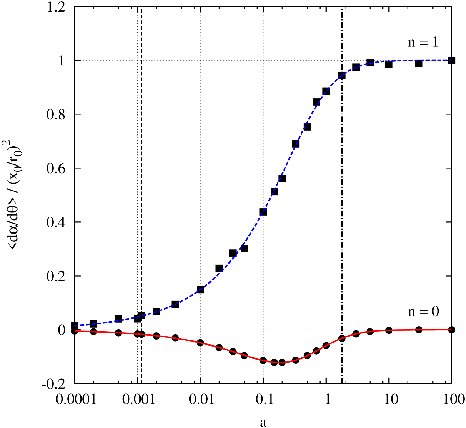
I employed a model homogeneous weak focusing all-electric ring with a radius of r0=40r_{0}=40 m for all of the numerical simulations reported below. In Figs. 1 and 2, I tracked betatron orbits and in Fig. 3 I tracked off-energy dispersion orbits. In all cases, the particles were launched with their spins pointing along the reference orbit.

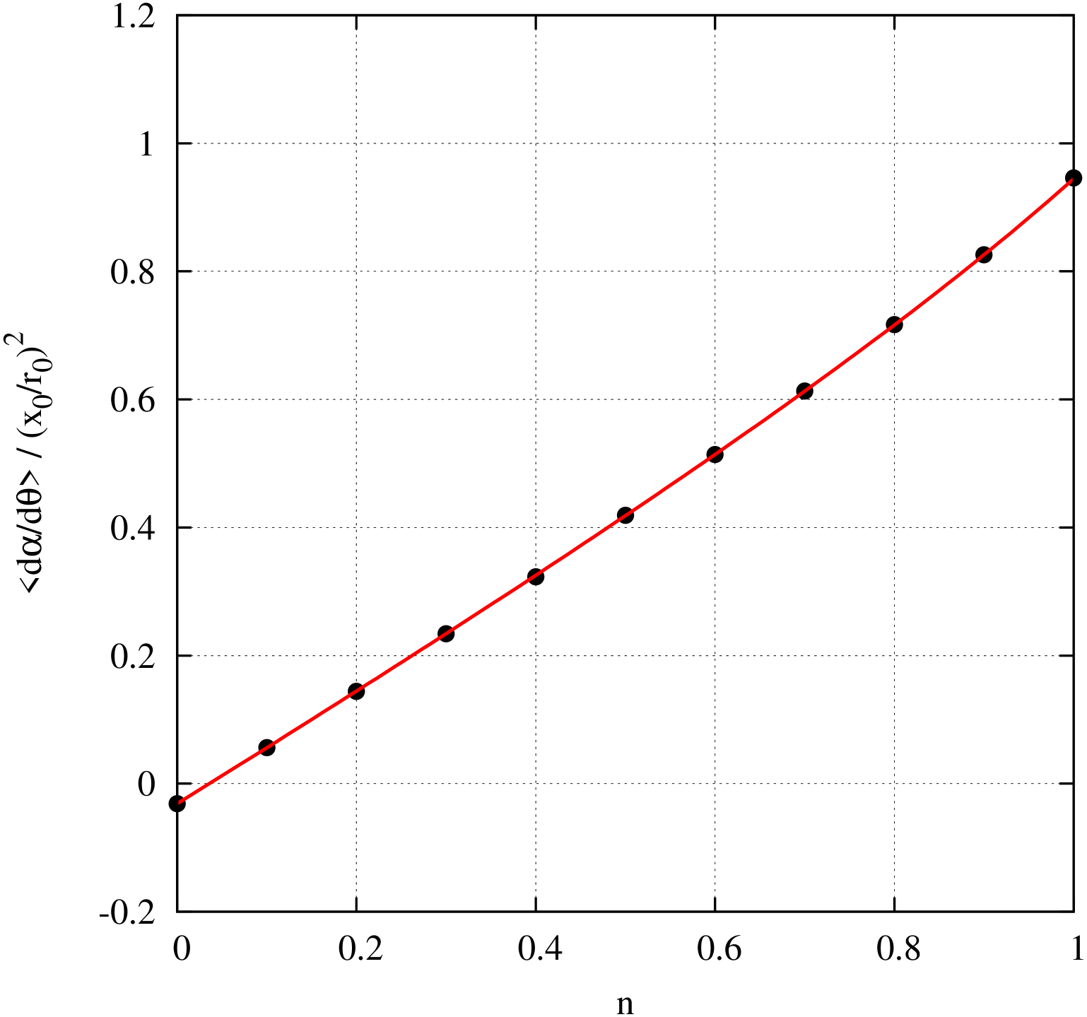
In both Figs. 1 and 2, I tracked one particle for one million turns, with an initial value x0=1x_{0}=1 mm and px0=0p_{x0}=0. The energy was H=H0=γ0mc2H=H_{0}=\gamma_{0}mc^{2}. A graph of dα/dθ/(x0/r0)2\langle d\alpha/d\theta\rangle/(x_{0}/r_{0})^{2} v. the magnetic moment anomaly aa is displayed in Fig. 1. The circles and squares are the tracking data for a field index of n=0n=0 and 1, viz. a logarithmic potential and the Kepler problem, respectively. The solid curves were plotted using the formulas in eq. (74). The dash and dotdash vertical lines denote the values of aa for a lepton and a proton, respectively. The agreement between the tracking data and the analytical formula is excellent. Next, in Fig. 2, I plotted a graph of dα/dθ/(x0/r0)2\langle d\alpha/d\theta\rangle/(x_{0}/r_{0})^{2} v. the field index nn, for 0n10\leq n\leq 1. I set the magnetic moment anomaly to that for a proton, i.e. a1.792847a\simeq 1.792847. The circles are the tracking data and the solid curve was plotted using eq. (73). The agreement between the tracking data and the analytical formula is excellent. Note that the curve is almost a straight line, and the spin decoherence rate increases with the field index.

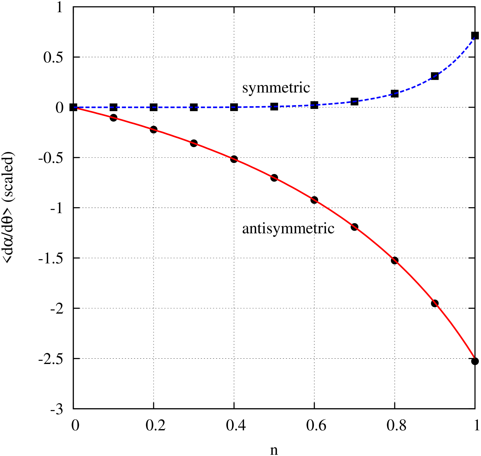
Next, I tracked the off-energy dispersion orbits. In this case the orbits are circles and no averaging is necessary. Since I derived the exact solution dαd/dθd\alpha_{d}/d\theta in eq. (31), there was no need to use a small value for λp\lambda_{p}. I set the magnetic moment anomaly to that for a proton and ΔH/H0=0.1\Delta H/H_{0}=0.1. Then λp=(ΔH/H0)/β020.279\lambda_{p}=(\Delta H/H_{0})/\beta_{0}^{2}\simeq 0.279. I tracked for ten thousand turns. The point was simply to demonstrate that the tracking program was capable of accepting such a large value of ΔH/H0\Delta H/H_{0} and the numerically computed orbits remained circular to high accuracy. (Typical results were |rrd|/r0<O(1013)|r-r_{d}|/r_{0}<O(10^{-13}) and |px|/p0<O(1014)|p_{x}|/p_{0}<O(10^{-14}).) The initial conditions were px0=0p_{x0}=0 and r=rdr=r_{d}, computed using eq. (30), by solving for γd\gamma_{d} using eqs. (26) and (29). I actually tracked two orbits, for ±λp\pm\lambda_{p} and computed the following scaled symmetric and antisymmetric parameters

𝒮=12λp2{dαddθ|λp+dαddθ|λp},\displaystyle\mathcal{S}=\frac{1}{2\lambda_{p}^{2}}\,\biggl{\{}\,\frac{d\alpha_{d}}{d\theta}\biggl{|}_{\lambda_{p}}+\frac{d\alpha_{d}}{d\theta}\biggl{|}_{-\lambda_{p}}\,\biggr{\}}\,, (157)
𝒜=12λp{dαddθ|λpdαddθ|λp}.\displaystyle\mathcal{A}=\frac{1}{2\lambda_{p}}\,\biggl{\{}\,\frac{d\alpha_{d}}{d\theta}\biggl{|}_{\lambda_{p}}-\frac{d\alpha_{d}}{d\theta}\biggl{|}_{-\lambda_{p}}\,\biggr{\}}\,. (158)

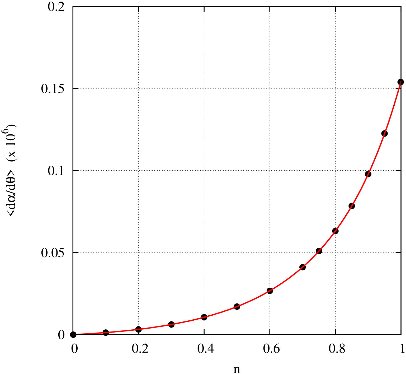
The antisymmetric and symmetric terms are essentially the coefficients of λp\lambda_{p} and λp2\lambda_{p}^{2} in a Taylor series expansion of dαd/dθd\alpha_{d}/d\theta in powers of λp\lambda_{p}. A graph of the (scaled) symmetric and antisymmetric terms in dαd/dθd\alpha_{d}/d\theta v. the field index nn is shown in Fig. 3. The squares and circles are the tracking data for the symmetric and antisymmetric terms viz. 𝒮\mathcal{S} and 𝒜\mathcal{A}, respectively. The solid and dashed curves were calculated using eq. (31). Note that in a real beam, where we expect λp=0\langle\lambda_{p}\rangle=0, the spin decoherence rate will be proportional to 𝒮\mathcal{S}. From Fig. 3, the value of 𝒮\mathcal{S} is very small for 0n0.60\leq n\lesssim 0.6 and then rises steeply with increasing nn.

In Fig. 4, I display simulation results for the spin decoherence due to synchrotron oscillations. The numerical tracking data are displayed as the circles in Fig. 4 and the solid line is the value of dαd/dθ\langle d\alpha_{d}/d\theta\rangle, calculated using eq. (38) with the averages derived in Section VI. One rf cavity was inserted in the ring, with a voltage of 11 MV and a harmonic number of h=1h=1. One particle was tracked with an initial energy offset given by λp0=2×10⁴\lambda_{p0}=2\times 10^{-4} and an initial time lag of zero. The orbital motion consisted of synchrotron oscillations only. There is excellent agreement between tracking and theory.

VIII Conclusion

I treated a model of relativistic charged particle motion in a horizontal plane in a central field of force. The model was a homogeneous weak focusing all-electric storage ring, with an arbitrary field index n0n\geq 0. I derived the expression for the spin decoherence rate, for both off-energy dispersion orbits and betatron oscillations. For the off-energy motion, the dispersion orbits are circles and I solved the problem exactly. For the betatron oscillations, I employed perturbation theory and canonical transformations. I have calculated the spin precession exactly for the relativistic Kepler problem ManeRelKepler . I verified that it confirmed the solution from perturbation theory. I displayed graphs of data from numerical tracking simulations, and demonstrated that the results matched well with the analytical calculations. In particular, I found that for a proton, the spin decoherence rate due to betatron oscillations increases approximately linearly with the field index nn. On the other hand, the spin decoherence rate due to the energy spread is very small for 0n0.60\leq n\lesssim 0.6 and then rises steeply with increasing nn.

I reprodced, with permission, Ivan Koop’s Koopprivcomm elegant analysis of motion in a vertical spiral in a logarithmic potential in Appendix A. I also derived the exact solution for the orbit and spin motion in a vertical spiral in a logarithmic potential, in Appendix B. Finally, a commentary on an analysis of the spin decoherence rate by Talman and Talman TalmanIPAC2012 is presented in some Appendices below, including a discussion of some quantitative errors in their analysis.

References

  • (1) S. R. Mane, Nucl. Inst. Meth. A 687 40–50 (2012).
  • (2) L. J. Laslett, ERAN-30 Note (1969) included in Selected Works of L. Jackson Laslett, LBL PUB-616, 1987, section 3, p. 13.
  • (3) S. R. Mane, arXiv:1403.5023 [physics.acc-ph] (2014). Available at http://arxiv.org/abs/1403.5023.
  • (4) S. R. Mane, Nucl. Inst. Meth. A, in press.
  • (5) I. A. Koop, private communication.
  • (6) R. Talman and J. Talman, Proceedings of IPAC2012, New Orleans, 3203–3207 (2012). Available at http://accelconf.web.cern.ch/AccelConf/IPAC2012/papers/thxb03.pdf.
  • (7) L. H. Thomas, Philos. Mag. 3 1–21 (1927).
  • (8) V. Bargmann, L. Michel and V. L. Telegdi, Phys. Rev. Lett. 2 435–436 (1959).
  • (9) S. R. Mane, Yu. M. Shatunov and K. Yokoya, Rep. Prog. Phys. 68, 1997–2265 (2005).
  • (10) S. R. Mane, arXiv:1403.7485 [physics.acc-ph] (2014). Available at http://arxiv.org/abs/1403.7485.

Appendix A Analysis by Koop of vertical spiral motion in a radial electric field

The following is reproduced with the kind permission of Ivan Koop Koopprivcomm . Koop solves for the particle kinetic energy and orbit radius for spiral motion in a logarithmic potential. Note that Koop employs the synchronous condition and uses ‘yy’ to denote motion along the reference orbit and denotes the pitch angle of the helix by θ\theta. The synchronous condition means that the projection of the motion in the horizontal plane circulates at the same frequency as the reference particle. (N.B.: it is easily deduced that the synchronous condition requires HH0H\neq H_{0}, i.e. Koop’s solution implies a nonzero energy offset.)

Consider a particle which spirals upward with a small angle θvz/vy\theta\approx v_{z}/v_{y} and still is synchronous with the RF frequency. That means:

vyr=v0r0=ω0.\frac{v_{y}}{r}=\frac{v_{0}}{r_{0}}=\omega_{0}\,. (159)

Let us show that rr0r\leq r_{0} and, hence, vyv0v_{y}\leq v_{0}. Again, from the equality of the centripetal force and of the radial electric force one can deduce:

γmvy2r=eE0r0r.\frac{\gamma mvy^{2}}{r}=\frac{eE_{0}r_{0}}{r}\,. (160)

Substituting into the above equation:

vy2(1+θ2)=11γ2,v_{y}^{2}(1+\theta^{2})=1-\frac{1}{\gamma^{2}}\,, (161)

one gets:

γ1γ=(1+θ2)(γ01γ0).\gamma-\frac{1}{\gamma}=(1+\theta^{2})\,\biggl{(}\gamma_{0}-\frac{1}{\gamma_{0}}\biggr{)}\,. (162)

Thus, the approximate value of the kinetic energy shift is equal to:

Δγγ=θ2γ021γ02+10.\frac{\Delta\gamma}{\gamma}=\theta^{2}\,\frac{\gamma_{0}^{2}-1}{\gamma_{0}^{2}+1}\geq 0\,. (163)

Now, from the equality γvy=γ0v02\gamma v_{y}=\gamma_{0}v_{0}^{2} one can deduce:

vy=v0γ0γv0(1Δγ2γ)=v0(1θ22γ021γ02+1).v_{y}=v_{0}\,\sqrt{\frac{\gamma_{0}}{\gamma}}\approx v_{0}\,\biggl{(}1-\frac{\Delta\gamma}{2\gamma}\biggr{)}=v_{0}\,\biggl{(}1-\frac{\theta^{2}}{2}\,\frac{\gamma_{0}^{2}-1}{\gamma_{0}^{2}+1}\biggr{)}\,. (164)

Same will be a relative change of the radius of an orbit:

r=r0vyv0=r0γ0γr0(1Δγ2γ)=r0(1θ22γ021γ02+1).r=r_{0}\,\frac{v_{y}}{v_{0}}=r_{0}\,\sqrt{\frac{\gamma_{0}}{\gamma}}\approx r_{0}\,\biggl{(}1-\frac{\Delta\gamma}{2\gamma}\biggr{)}=r_{0}\,\biggl{(}1-\frac{\theta^{2}}{2}\,\frac{\gamma_{0}^{2}-1}{\gamma_{0}^{2}+1}\biggr{)}\,. (165)

Appendix B Logarithmic potential

I solve for both the orbit and spin for motion in a vertical spiral in a logarithmic potential. The field and potential are, for all orbits

𝑬=E0r0r,V=E0r0lnrr0.\bm{E}=-\frac{E_{0}r_{0}}{r}\,,\qquad V=E_{0}r_{0}\,\ln\frac{r}{r_{0}}\,. (166)

There is no vertical focusing. The vertical momentum is a dynamical invariant pz=pz0=constp_{z}=p_{z0}=\textrm{const}. Suppose the trajectory is a vertical spiral, of radius rr_{*}, say, hence there is no radial momentum, i.e. pr=0p_{r}=0. Let the pitch angle of the spiral be ϑ\vartheta_{*}. Then rr_{*} and ϑ\vartheta_{*} are both constants of the motion. (Note that in general rr0r_{*}\neq r_{0}; this will be discussed below.) The centripetal force yields

mγvθ2r=eE0r0r.\frac{m\gamma v_{\theta}^{2}}{r}=\frac{eE_{0}r_{0}}{r}\,. (167)

Hence using eE0r0=mc2γ0β02eE_{0}r_{0}=mc^{2}\gamma_{0}\beta_{0}^{2}, we deduce γβθ2=γ0β02\gamma\beta_{\theta}^{2}=\gamma_{0}\beta_{0}^{2}. Now by definition tanϑ=βz/βθ\tan\vartheta_{*}=\beta_{z}/\beta_{\theta}, so βθ=βcosϑ\beta_{\theta}=\beta\cos\vartheta_{*}. Hence

γ1γ=γβ2=γ0β02cos2ϑ.\gamma-\frac{1}{\gamma}=\gamma\beta^{2}=\frac{\gamma_{0}\beta_{0}^{2}}{\cos^{2}\vartheta_{*}}\,. (168)

Hence the value of γ\gamma is determined solely by the reference value γ0\gamma_{0} and the pitch angle ϑ\vartheta_{*}, and does not depend on orbit radius rr_{*} or the total energy HH. Next

γ2γγ0β02cos2ϑ1=0.\gamma^{2}-\gamma\,\frac{\gamma_{0}\beta_{0}^{2}}{\cos^{2}\vartheta_{*}}-1=0\,. (169)

This can be solved exactly. We want the positive root, say γ\gamma_{*},

γ=12[γ0β02cos2ϑ+γ02β04cos4ϑ+4].\gamma_{*}=\frac{1}{2}\,\biggl{[}\,\frac{\gamma_{0}\beta_{0}^{2}}{\cos^{2}\vartheta_{*}}+\sqrt{\frac{\gamma_{0}^{2}\beta_{0}^{4}}{\cos^{4}\vartheta_{*}}+4}\,\biggr{]}\,. (170)

We can also solve approximately for |ϑ|1|\vartheta_{*}|\ll 1. Using eq. (168) and writing γ=γ0+Δγ\gamma_{*}=\gamma_{0}+\Delta\gamma_{*},

γ01γ0+(1+1γ02)Δγ\displaystyle\gamma_{0}-\frac{1}{\gamma_{0}}+\Bigl{(}1+\frac{1}{\gamma_{0}^{2}}\Bigr{)}\Delta\gamma_{*} γ0β02cos2ϑ,\displaystyle\simeq\frac{\gamma_{0}\beta_{0}^{2}}{\cos^{2}\vartheta_{*}}\,, (171)
γ0β02+γ02+1γ02Δγ\displaystyle\gamma_{0}\beta_{0}^{2}+\frac{\gamma_{0}^{2}+1}{\gamma_{0}^{2}}\,\Delta\gamma_{*} γ0β02cos2ϑ,\displaystyle\simeq\frac{\gamma_{0}\beta_{0}^{2}}{\cos^{2}\vartheta_{*}}\,, (172)
(γ02+1)Δγγ0\displaystyle(\gamma_{0}^{2}+1)\,\frac{\Delta\gamma_{*}}{\gamma_{0}} γ02β02tan2ϑ,\displaystyle\simeq\gamma_{0}^{2}\beta_{0}^{2}\,\tan^{2}\vartheta_{*}\,, (173)
Δγγ0\displaystyle\frac{\Delta\gamma_{*}}{\gamma_{0}} ϑ2γ021γ02+1.\displaystyle\simeq\vartheta_{*}^{2}\,\frac{\gamma_{0}^{2}-1}{\gamma_{0}^{2}+1}\,. (174)

We determine the radius from the total energy HH. We do not need to constrain the energy to be H0H_{0}; we can permit an offset ΔH/H0=β02λp\Delta H/H_{0}=\beta_{0}^{2}\,\lambda_{p}. Then, using H=γmc2+eΦH=\gamma mc^{2}+e\Phi,

H\displaystyle H =γmc2+eE0r0lnrr0,\displaystyle=\gamma_{*}mc^{2}+eE_{0}r_{0}\,\ln\frac{r_{*}}{r_{0}}\,, (175)
γ0(1+β02λp)\displaystyle\gamma_{0}(1+\beta_{0}^{2}\lambda_{p}) =γ0+Δγ+γ0β02lnrr0,\displaystyle=\gamma_{0}+\Delta\gamma_{*}+\gamma_{0}\beta_{0}^{2}\,\ln\frac{r_{*}}{r_{0}}\,, (176)
λpΔγγ0β02\displaystyle\lambda_{p}-\frac{\Delta\gamma_{*}}{\gamma_{0}\beta_{0}^{2}} =lnrr0,\displaystyle=\ln\frac{r_{*}}{r_{0}}\,, (177)
r\displaystyle r_{*} =r0eλpΔγ/(γ0β02).\displaystyle=r_{0}\,e^{\lambda_{p}-\Delta\gamma_{*}/(\gamma_{0}\beta_{0}^{2})}\,. (178)

This is the exact solution. Note that in general rr0r_{*}\neq r_{0}. Next we treat the spin motion and the helicity. Recall that

ddt(𝒔𝜷^)=emc(a1β2γ2)(𝜷×𝑬)(𝒔×𝜷^).\frac{d\ }{dt}(\bm{s}\cdot\hat{\bm{\beta}})=\frac{e}{mc}\biggl{(}a-\frac{1}{\beta^{2}\gamma^{2}}\biggr{)}(\bm{\beta}\times\bm{E})\cdot(\bm{s}\times\hat{\bm{\beta}})\,. (179)

In this model 𝑬𝒓^\bm{E}\parallel\hat{\bm{r}} and 𝜷\bm{\beta} has no radial component, so 𝑬𝜷=0\bm{E}\cdot\bm{\beta}=0, so

(𝜷×𝑬)(𝒔×𝜷^)=𝜷𝒔𝑬𝜷^𝜷𝜷^𝑬𝒔=Eβ𝒔𝒓^(\bm{\beta}\times\bm{E})\cdot(\bm{s}\times\hat{\bm{\beta}})=\bm{\beta}\cdot\bm{s}\,\bm{E}\cdot\hat{\bm{\beta}}-\bm{\beta}\cdot\hat{\bm{\beta}}\,\bm{E}\cdot\bm{s}=-E\beta_{*}\,\bm{s}\cdot\hat{\bm{r}} (180)

Hence using dθ/dt=cβθ/rd\theta/dt=c\beta_{\theta}/r_{*},

ddθ(𝒔𝜷^)=rcβθeEβmc(a1β2γ2)𝒔𝒓^=eE0r0mc2cosϑ(a1β2γ2)𝒔𝒓^=γ0β02cosϑ(a1β2γ2)𝒔𝒓^=1γ0cosϑ(1β02γ02β2γ2)𝒔𝒓^.\begin{split}\frac{d\ }{d\theta}(\bm{s}\cdot\hat{\bm{\beta}})&=-\frac{r_{*}}{c\beta_{\theta}}\,\frac{eE\beta_{*}}{mc}\biggl{(}a-\frac{1}{\beta_{*}^{2}\gamma_{*}^{2}}\biggr{)}\,\bm{s}\cdot\hat{\bm{r}}\\ &=\frac{eE_{0}r_{0}}{mc^{2}\cos\vartheta_{*}}\biggl{(}a-\frac{1}{\beta_{*}^{2}\gamma_{*}^{2}}\biggr{)}\,\bm{s}\cdot\hat{\bm{r}}\\ &=\frac{\gamma_{0}\beta_{0}^{2}}{\cos\vartheta_{*}}\,\biggl{(}a-\frac{1}{\beta_{*}^{2}\gamma_{*}^{2}}\biggr{)}\,\bm{s}\cdot\hat{\bm{r}}\\ &=\frac{1}{\gamma_{0}\cos\vartheta_{*}}\,\biggl{(}1-\frac{\beta_{0}^{2}\gamma_{0}^{2}}{\beta_{*}^{2}\gamma_{*}^{2}}\biggr{)}\,\bm{s}\cdot\hat{\bm{r}}\,.\end{split} (181)

In the last line, the value of aa was set using the magic gamma a=1/(β02γ02)a=1/(\beta_{0}^{2}\gamma_{0}^{2}). Notice that 𝒔𝒓^\bm{s}\cdot\hat{\bm{r}} appears on the right-hand side of the above equation. Hence we cannot simply write 𝒔𝜷^=cosα\bm{s}\cdot\hat{\bm{\beta}}=\cos\alpha and derive an equation purely for dα/dθd\alpha/d\theta as was done for case of motion in the horizontal plane. We must solve for the spin motion explicitly. We do so as follows. In the absence of a magnetic field, the spin precession equation of motion is

d𝒔dt=𝛀×𝒔=emc(a+1γ+1)(𝜷×𝑬)×𝒔.\frac{d\bm{s}}{dt}=\bm{\Omega}\times\bm{s}=\frac{e}{mc}\,\biggl{(}a+\frac{1}{\gamma+1}\biggr{)}\,(\bm{\beta}\times\bm{E})\times\bm{s}\,. (182)

The spin precession vector 𝛀\bm{\Omega} points along 𝜷×𝑬\bm{\beta}\times\bm{E}. Recall that 𝑬\bm{E} points radially and 𝜷\bm{\beta} points along the tangent to the orbit helix, hence in a cylindrical polar coordinate system, 𝜷×𝑬\bm{\beta}\times\bm{E} has fixed (in time) components along 𝜽^\hat{\bm{\theta}} and 𝒛^\hat{\bm{z}}, viz.

𝜷×𝑬𝜷×𝒓^=(βθ𝜽^+βz𝒛^)×𝒓^=βθ𝒛^+βz𝜽^.\bm{\beta}\times\bm{E}\;\parallel\;\bm{\beta}\times\hat{\bm{r}}=(\beta_{\theta}\,\hat{\bm{\theta}}+\beta_{z}\,\hat{\bm{z}})\times\hat{\bm{r}}=-\beta_{\theta}\,\hat{\bm{z}}+\beta_{z}\,\hat{\bm{\theta}}\,. (183)

Next we need to express the evolution of the spin components in cylindrical polar coordinates

d𝒔dt=dsrdt𝒓^+dsθdt𝜽^+dszdt𝒛^+srd𝒓^dt+sθd𝜽^dt=dsrdt𝒓^+dsθdt𝜽^+dszdt𝒛^+vθr𝒛^×𝒔.\begin{split}\frac{d\bm{s}}{dt}&=\frac{ds_{r}}{dt}\,\hat{\bm{r}}+\frac{ds_{\theta}}{dt}\,\hat{\bm{\theta}}+\frac{ds_{z}}{dt}\,\hat{\bm{z}}+s_{r}\,\frac{d\hat{\bm{r}}}{dt}+s_{\theta}\,\frac{d\hat{\bm{\theta}}}{dt}\\ &=\frac{ds_{r}}{dt}\,\hat{\bm{r}}+\frac{ds_{\theta}}{dt}\,\hat{\bm{\theta}}+\frac{ds_{z}}{dt}\,\hat{\bm{z}}+\frac{v_{\theta}}{r}\,\hat{\bm{z}}\times\bm{s}\,.\end{split} (184)

Then we derive an ‘effective’ spin precession vector as follows

dsrdθ𝒓^+dsθdθ𝜽^+dszdθ𝒛^=(rvθ𝛀𝒛^)×𝒔𝛀¯×𝒔.\frac{ds_{r}}{d\theta}\,\hat{\bm{r}}+\frac{ds_{\theta}}{d\theta}\,\hat{\bm{\theta}}+\frac{ds_{z}}{d\theta}\,\hat{\bm{z}}=\Bigl{(}\frac{r}{v_{\theta}}\,\bm{\Omega}-\hat{\bm{z}}\Bigr{)}\times\bm{s}\equiv\bar{\bm{\Omega}}\times\bm{s}\,. (185)

In the language of General Relativity, this is a covariant derivative; we have subtracted contribution from the time variation of the basis vectors 𝒓^\hat{\bm{r}} and 𝜽^\hat{\bm{\theta}}. Then

𝛀¯=rvθ𝛀𝒛^=ermc2βθ(a+1γ+1)(𝜷×𝑬)𝒛^=eE0r0mc2βθ(a+1γ+1)(βθ𝒛^+βz𝜽^)𝒛^=γ0β02[(a+1γ+11γ0β02)𝒛^(a+1γ+1)βzβθ𝜽^].\begin{split}\bar{\bm{\Omega}}&=\frac{r}{v_{\theta}}\,\bm{\Omega}-\hat{\bm{z}}\\ &=\frac{er_{*}}{mc^{2}\beta_{\theta}}\,\biggl{(}a+\frac{1}{\gamma+1}\biggr{)}\,(\bm{\beta}\times\bm{E})-\hat{\bm{z}}\\ &=-\frac{eE_{0}r_{0}}{mc^{2}\beta_{\theta}}\,\biggl{(}a+\frac{1}{\gamma_{*}+1}\biggr{)}\,(-\beta_{\theta}\,\hat{\bm{z}}+\beta_{z}\,\hat{\bm{\theta}})-\hat{\bm{z}}\\ &=\gamma_{0}\beta_{0}^{2}\,\biggl{[}\biggl{(}a+\frac{1}{\gamma_{*}+1}-\frac{1}{\gamma_{0}\beta_{0}^{2}}\biggr{)}\,\hat{\bm{z}}-\biggl{(}a+\frac{1}{\gamma_{*}+1}\biggr{)}\frac{\beta_{z}}{\beta_{\theta}}\,\hat{\bm{\theta}}\biggr{]}\,.\end{split} (186)

This has the significant feature that the components of 𝛀¯\bar{\bm{\Omega}} are constant in time (or θ\theta), when expressed in cylindrical polar coordinates. Hence the spin components (sr,sθ,sz)(s_{r},s_{\theta},s_{z}) precess in a plane normal to 𝛀¯\bar{\bm{\Omega}}, at angular frequency |𝛀¯||\bar{\bm{\Omega}}|. (Note that in the lab frame, the ‘plane’ itself rotates around the vertical axis at the angular frequency vθ/rv_{\theta}/r_{*}.) Note also that the orientation of this plane is not equal to the pitch angle ϑ\vartheta_{*} of the orbital motion. Unlike the case of motion in the horizontal plane, the spin does not precess in the same plane as the orbit. Let 𝛀¯\bar{\bm{\Omega}} be oriented at an angle φ\varphi_{*} to the horizontal. Then define Ω¯\bar{\Omega} via

𝛀¯=Ω¯(cosφ𝜽^+sinφ𝒛^).\bar{\bm{\Omega}}=\bar{\Omega}\,(\cos\varphi_{*}\,\hat{\bm{\theta}}+\sin\varphi_{*}\,\hat{\bm{z}})\,. (187)

Then

tanφ=a+1/(γ+1)1/(γ0β02)a+1/(γ+1)βθβz.\tan\varphi_{*}=-\frac{a+1/(\gamma_{*}+1)-1/(\gamma_{0}\beta_{0}^{2})}{a+1/(\gamma_{*}+1)}\,\frac{\beta_{\theta}}{\beta_{z}}\,. (188)

Let us define a right-handed orthonormal basis (𝜻1,𝜻2,𝜻3)(\bm{\zeta}_{1},\bm{\zeta}_{2},\bm{\zeta}_{3}) as follows

𝜻1\displaystyle\bm{\zeta}_{1} =𝒓^,\displaystyle=\phantom{-}\hat{\bm{r}}\,, (189a)
𝜻2\displaystyle\bm{\zeta}_{2} =cosφ𝜽^+sinφ𝒛^,\displaystyle=\phantom{-}\cos\varphi_{*}\,\hat{\bm{\theta}}+\sin\varphi_{*}\,\hat{\bm{z}}\,, (189b)
𝜻3\displaystyle\bm{\zeta}_{3} =sinφ𝜽^+cosφ𝒛^.\displaystyle=-\sin\varphi_{*}\,\hat{\bm{\theta}}+\cos\varphi_{*}\,\hat{\bm{z}}\,. (189c)

Then 𝜻1𝑬\bm{\zeta}_{1}\parallel\bm{E}, 𝜻2𝛀¯\bm{\zeta}_{2}\parallel\bar{\bm{\Omega}} and 𝜻3=𝜻1×𝜻2\bm{\zeta}_{3}=\bm{\zeta}_{1}\times\bm{\zeta}_{2}. Our interest is in the case when the spin points initially along the reference orbit

𝒔(0)=𝜽^=cosφ𝜻2sinφ𝜻3.\bm{s}(0)=\hat{\bm{\theta}}=\cos\varphi_{*}\,\bm{\zeta}_{2}-\sin\varphi_{*}\,\bm{\zeta}_{3}\,. (190)

Since 𝛀¯\bar{\bm{\Omega}} has constant (in θ\theta) components in cylindrical polar coordinates, the component of 𝒔\bm{s} parallel to 𝛀¯\bar{\bm{\Omega}} is invariant, and the other components of 𝒔\bm{s} precess in the (𝜻1,𝜻3)(\bm{\zeta}_{1},\bm{\zeta}_{3}) plane at the angular frequency Ω¯\bar{\Omega}. Hence

𝒔=cosφ𝜻2sinφ[cos(Ω¯θ)𝜻3+sin(Ω¯θ)𝜻1].\bm{s}=\cos\varphi_{*}\,\bm{\zeta}_{2}-\sin\varphi_{*}\,\bigl{[}\,\cos(\bar{\Omega}\theta)\bm{\zeta}_{3}+\sin(\bar{\Omega}\theta)\bm{\zeta}_{1}\,\bigr{]}\,. (191)

Then

𝒔𝒓^=𝒔𝜻1=sinφsin(Ω¯θ).\bm{s}\cdot\hat{\bm{r}}=\bm{s}\cdot\bm{\zeta}_{1}=-\sin\varphi_{*}\,\sin(\bar{\Omega}\theta)\,. (192)

We can now use this in eq. (181). However, since we know 𝒔\bm{s} as a function of θ\theta, let us solve for the evolution of the helicity directly. Using 𝜷^=cosϑ𝜽^+sinϑ𝒛^\hat{\bm{\beta}}=\cos\vartheta_{*}\,\hat{\bm{\theta}}+\sin\vartheta_{*}\,\hat{\bm{z}}, the helicity is

𝒔𝜷^=cosφ𝜻2𝜷^sinφcos(Ω¯θ)𝜻3𝜷^=cosφcos(φϑ)+sinφsin(φϑ)cos(Ω¯θ).\begin{split}\bm{s}\cdot\hat{\bm{\beta}}&=\cos\varphi_{*}\,\bm{\zeta}_{2}\cdot\hat{\bm{\beta}}-\sin\varphi_{*}\,\cos(\bar{\Omega}\theta)\,\bm{\zeta}_{3}\cdot\hat{\bm{\beta}}\\ &=\cos\varphi_{*}\,\cos(\varphi_{*}-\vartheta_{*})+\sin\varphi_{*}\,\sin(\varphi_{*}-\vartheta_{*})\,\cos(\bar{\Omega}\theta)\,.\end{split} (193)

Hence

ddθ(𝒔𝜷^)=Ω¯sinφsin(φϑ)sin(Ω¯θ).\frac{d\ }{d\theta}(\bm{s}\cdot\hat{\bm{\beta}})=-\bar{\Omega}\,\sin\varphi_{*}\,\sin(\varphi_{*}-\vartheta_{*})\,\sin(\bar{\Omega}\theta)\,. (194)

Note also, using 𝒔𝜷^=cosα\bm{s}\cdot\hat{\bm{\beta}}=\cos\alpha that d(𝒔𝜷^)/dθ=sinα(dα/dθ)d(\bm{s}\cdot\hat{\bm{\beta}})/d\theta=-\sin\alpha\,(d\alpha/d\theta). Hence

dαdθ=Ω¯sinφsin(φϑ)sin(Ω¯θ)sinα.\frac{d\alpha}{d\theta}=\bar{\Omega}\,\frac{\sin\varphi_{*}\,\sin(\varphi_{*}-\vartheta_{*})\,\sin(\bar{\Omega}\theta)}{\sin\alpha}\,. (195)

We need an expression for sinα\sin\alpha, but only have an expression for cosα=𝒔𝜷^\cos\alpha=\bm{s}\cdot\hat{\bm{\beta}}. Using sin2α=1cos2α=1(𝒔𝜷^)2\sin^{2}\alpha=1-\cos^{2}\alpha=1-(\bm{s}\cdot\hat{\bm{\beta}})^{2}, we provisionally write

dαdθ=Ω¯sinφsin(φϑ)sin(Ω¯θ)1(𝒔𝜷^)2.\frac{d\alpha}{d\theta}=\bar{\Omega}\,\frac{\sin\varphi_{*}\,\sin(\varphi_{*}-\vartheta_{*})\,\sin(\bar{\Omega}\theta)}{\sqrt{1-(\bm{s}\cdot\hat{\bm{\beta}})^{2}}}\,. (196)

The provision is that sinα\sin\alpha changes sign according as α\alpha is positive or negative, but the square root in the denominator is always positive. Hence we must exercise some care to average over the orbit. (Note also that because the angular velocity is constant, an average over tt is equivalent to an average over θ\theta.) Hence define ϕ~=Ω¯θ\tilde{\phi}=\bar{\Omega}\theta and

χ=sinφsin(φϑ)sinϕ~1(cosφcos(φϑ)+sinφsin(φϑ)cosϕ~)2.\chi=\frac{\sin\varphi_{*}\,\sin(\varphi_{*}-\vartheta_{*})\,\sin\tilde{\phi}}{\sqrt{1-(\cos\varphi_{*}\,\cos(\varphi_{*}-\vartheta_{*})+\sin\varphi_{*}\,\sin(\varphi_{*}-\vartheta_{*})\,\cos\tilde{\phi})^{2}}}\,. (197)

If we average this over a full period of ϕ~\tilde{\phi}, the average will vanish because the numerator is antisymmetric and the denominator is symmetric under a transformation ϕ~ϕ~\tilde{\phi}\to-\tilde{\phi}. We obtain the correct answer by averaging over half a period 0ϕ~π0\leq\tilde{\phi}\leq\pi

χ=1π0πχ𝑑ϕ~.\langle\chi\rangle=\frac{1}{\pi}\,\int_{0}^{\pi}\chi\,d\tilde{\phi}\,. (198)

We employ the substitution

u=cosφcos(φϑ)+sinφsin(φϑ)cosϕ~u=\cos\varphi_{*}\,\cos(\varphi_{*}-\vartheta_{*})+\sin\varphi_{*}\,\sin(\varphi_{*}-\vartheta_{*})\,\cos\tilde{\phi} (199)

The limits on uu are, for ϕ~=0\tilde{\phi}=0 and π\pi respectively,

u0\displaystyle u_{0} =cosφcos(φϑ)+sinφsin(φϑ)=cosϑ,\displaystyle=\cos\varphi_{*}\,\cos(\varphi_{*}-\vartheta_{*})+\sin\varphi_{*}\,\sin(\varphi_{*}-\vartheta_{*})=\cos\vartheta_{*}\,, (200a)
uπ\displaystyle u_{\pi} =cosφcos(φϑ)sinφsin(φϑ)=cos(2φϑ).\displaystyle=\cos\varphi_{*}\,\cos(\varphi_{*}-\vartheta_{*})-\sin\varphi_{*}\,\sin(\varphi_{*}-\vartheta_{*})=\cos(2\varphi_{*}-\vartheta_{*})\,. (200b)

Then

χ=1πu0uπdu1u2=1π[cos1u]u0uπ=1π[(2φϑ)ϑ]=2(φϑ)π.\begin{split}\langle\chi\rangle&=-\frac{1}{\pi}\,\int_{u_{0}}^{u_{\pi}}\frac{du}{\sqrt{1-u^{2}}}\\ &=\frac{1}{\pi}\,\biggl{[}\,\cos^{-1}u\,\biggr{]}_{u_{0}}^{u_{\pi}}\\ &=\frac{1}{\pi}\,\biggl{[}\,(2\varphi_{*}-\vartheta_{*})-\vartheta_{*}\,\biggr{]}\\ &=\frac{2(\varphi_{*}-\vartheta_{*})}{\pi}\,.\end{split} (201)

Hence

dαdθ=2(φϑ)πΩ¯.\biggl{\langle}\frac{d\alpha}{d\theta}\biggr{\rangle}=\frac{2(\varphi_{*}-\vartheta_{*})}{\pi}\,\bar{\Omega}\,. (202)

This is a formally exact solution; all quantities in the above expression are known exactly, in principle. Note also from eq. (186) that both Ω¯\bar{\Omega} and φ\varphi_{*} depend only on the reference value γ0\gamma_{0} and the pitch angle of the helix ϑ\vartheta_{*}. Hence we do not require knowledge of the orbit radius, nor the total energy, to derive the above solution.

Let us now evaluate Ω¯\bar{\Omega} and φ\varphi_{*} approximately, for |ϑ|1|\vartheta_{*}|\ll 1. Note that by construction, 𝛀¯\bar{\bm{\Omega}} vanishes on the reference orbit. Hence off-axis, 𝛀¯\bar{\bm{\Omega}} is a small quantity. We determine the components of 𝛀¯\bar{\bm{\Omega}} as follows. First, using a=1/(γ021)a=1/(\gamma_{0}^{2}-1),

a+1γ+11γ0β02=1γ+1γ01γ021=1γ+11γ0+1=γ0γ(γ+1)(γ0+1)γ0(γ0+1)2Δγγ0ϑ2γ0(γ0+1)2γ021γ02+1ϑ2γ0γ02+1γ01γ0+1.\begin{split}a+\frac{1}{\gamma_{*}+1}-\frac{1}{\gamma_{0}\beta_{0}^{2}}&=\frac{1}{\gamma_{*}+1}-\frac{\gamma_{0}-1}{\gamma_{0}^{2}-1}\\ &=\frac{1}{\gamma_{*}+1}-\frac{1}{\gamma_{0}+1}\\ &=\frac{\gamma_{0}-\gamma_{*}}{(\gamma_{*}+1)(\gamma_{0}+1)}\\ &\simeq-\frac{\gamma_{0}}{(\gamma_{0}+1)^{2}}\,\frac{\Delta\gamma_{*}}{\gamma_{0}}\\ &\simeq-\vartheta_{*}^{2}\,\frac{\gamma_{0}}{(\gamma_{0}+1)^{2}}\,\frac{\gamma_{0}^{2}-1}{\gamma_{0}^{2}+1}\\ &\simeq-\vartheta_{*}^{2}\,\frac{\gamma_{0}}{\gamma_{0}^{2}+1}\,\frac{\gamma_{0}-1}{\gamma_{0}+1}\,.\end{split} (203)

Next

a+1γ+11β02γ02+1γ0+1=1γ021+γ01γ021=γ0γ021=1γ0β02.a+\frac{1}{\gamma_{*}+1}\simeq\frac{1}{\beta_{0}^{2}\gamma_{0}^{2}}+\frac{1}{\gamma_{0}+1}=\frac{1}{\gamma_{0}^{2}-1}+\frac{\gamma_{0}-1}{\gamma_{0}^{2}-1}=\frac{\gamma_{0}}{\gamma_{0}^{2}-1}=\frac{1}{\gamma_{0}\beta_{0}^{2}}\,. (204)

Substituting in eq. (186),

𝛀¯=γ0β02[(a+1γ+11γβθ2)𝒛^(a+1γ+1)βzβθ𝜽^]γ0β02[ϑ2γ0γ02+1γ01γ0+1𝒛^+1γ0β02ϑ𝜽^]ϑ2(γ01)2γ02+1𝒛^ϑ𝜽^.\begin{split}\bar{\bm{\Omega}}&=\gamma_{0}\beta_{0}^{2}\,\biggl{[}\biggl{(}a+\frac{1}{\gamma_{*}+1}-\frac{1}{\gamma_{*}\beta_{\theta}^{2}}\biggr{)}\hat{\bm{z}}-\biggl{(}a+\frac{1}{\gamma_{*}+1}\biggr{)}\frac{\beta_{z}}{\beta_{\theta}}\hat{\bm{\theta}}\biggr{]}\\ &\simeq-\gamma_{0}\beta_{0}^{2}\,\biggl{[}\,\vartheta_{*}^{2}\,\frac{\gamma_{0}}{\gamma_{0}^{2}+1}\,\frac{\gamma_{0}-1}{\gamma_{0}+1}\,\hat{\bm{z}}+\frac{1}{\gamma_{0}\beta_{0}^{2}}\,\vartheta_{*}\,\hat{\bm{\theta}}\,\biggr{]}\\ &\simeq-\vartheta_{*}^{2}\,\frac{(\gamma_{0}-1)^{2}}{\gamma_{0}^{2}+1}\,\hat{\bm{z}}-\vartheta_{*}\,\hat{\bm{\theta}}\,.\end{split} (205)

The horizontal and vertical components of 𝛀¯\bar{\bm{\Omega}} are of the first and second order in small quantities, respectively. Hence for a small orbital pitch angle |ϑ|1|\vartheta_{*}|\ll 1, 𝛀¯\bar{\bm{\Omega}} is almost horizontal. This demonstrates that the orientation of the off-axis components of the spin precession vector can be counterintuitive, for the various modes of off-axis orbital motion. For |ϑ|1|\vartheta_{*}|\ll 1,

Ω¯\displaystyle\bar{\Omega} ϑ,\displaystyle\simeq-\vartheta_{*}\,, (206)
φtanφ\displaystyle\varphi_{*}\simeq\tan\varphi_{*} (γ01)2γ02+1ϑ,\displaystyle\simeq\frac{(\gamma_{0}-1)^{2}}{\gamma_{0}^{2}+1}\,\vartheta_{*}\,, (207)
φϑ\displaystyle\varphi_{*}-\vartheta_{*} 2γ0γ02+1ϑ.\displaystyle\simeq-\frac{2\gamma_{0}}{\gamma_{0}^{2}+1}\,\vartheta_{*}\,. (208)

We now approximate for small |ϑ||\vartheta_{*}|.

dαdθ4ϑ2πγ0γ02+1.\biggl{\langle}\frac{d\alpha}{d\theta}\biggr{\rangle}\simeq\frac{4\vartheta_{*}^{2}}{\pi}\,\frac{\gamma_{0}}{\gamma_{0}^{2}+1}\,. (209)

As stated above, this depends only on the reference value γ0\gamma_{0} and the pitch angle of the helix ϑ\vartheta_{*}, but not on the orbit radius rr_{*} or the total energy HH.

For the sake of completeness, let us derive the above result by following the formal procedure using eq. (181). Using eq. (192),

dαdθ=1γ0cosϑ(1β02γ02β2γ2)sinφsin(Ω¯θ)1(𝒔𝜷^)2=1γ0cosϑsin(φϑ)(1β02γ02β2γ2)χ.\begin{split}\frac{d\alpha}{d\theta}&=\frac{1}{\gamma_{0}\cos\vartheta_{*}}\,\biggl{(}1-\frac{\beta_{0}^{2}\gamma_{0}^{2}}{\beta_{*}^{2}\gamma_{*}^{2}}\biggr{)}\,\frac{\sin\varphi_{*}\,\sin(\bar{\Omega}\theta)}{\sqrt{1-(\bm{s}\cdot\hat{\bm{\beta}})^{2}}}\\ &=\frac{1}{\gamma_{0}\cos\vartheta_{*}\sin(\varphi_{*}-\vartheta_{*})}\,\biggl{(}1-\frac{\beta_{0}^{2}\gamma_{0}^{2}}{\beta_{*}^{2}\gamma_{*}^{2}}\biggr{)}\,\chi\,.\end{split} (210)

Then use eq. (201) to deduce the average

dαdθ=2πγ0cosϑ(1β02γ02β2γ2)φϑsin(φϑ).\biggl{\langle}\frac{d\alpha}{d\theta}\biggr{\rangle}=\frac{2}{\pi\gamma_{0}\cos\vartheta_{*}}\,\biggl{(}1-\frac{\beta_{0}^{2}\gamma_{0}^{2}}{\beta_{*}^{2}\gamma_{*}^{2}}\biggr{)}\,\frac{\varphi_{*}-\vartheta_{*}}{\sin(\varphi_{*}-\vartheta_{*})}\,. (211)

This is also a formally exact solution. Next we need

1β02γ02β2γ2=1γ021γ21γ2γ02β02γ02(1+Δγ/γ0)21β022β02Δγγ0.1-\frac{\beta_{0}^{2}\gamma_{0}^{2}}{\beta_{*}^{2}\gamma_{*}^{2}}=1-\frac{\gamma_{0}^{2}-1}{\gamma_{*}^{2}-1}\simeq\frac{\gamma_{*}^{2}-\gamma_{0}^{2}}{\beta_{0}^{2}\gamma_{0}^{2}}\simeq\frac{(1+\Delta\gamma_{*}/\gamma_{0})^{2}-1}{\beta_{0}^{2}}\simeq\frac{2}{\beta_{0}^{2}}\,\frac{\Delta\gamma_{*}}{\gamma_{0}}\,. (212)

Then for |ϑ|1|\vartheta_{*}|\ll 1,

dαdθ4ϑ2πγ0β02cosϑγ021γ02+1φϑsin(φϑ)4ϑ2πγ0γ02+1.\begin{split}\biggl{\langle}\frac{d\alpha}{d\theta}\biggr{\rangle}&\simeq\frac{4\vartheta_{*}^{2}}{\pi\gamma_{0}\beta_{0}^{2}\cos\vartheta_{*}}\,\frac{\gamma_{0}^{2}-1}{\gamma_{0}^{2}+1}\,\frac{\varphi_{*}-\vartheta_{*}}{\sin(\varphi_{*}-\vartheta_{*})}\\ &\simeq\frac{4\vartheta_{*}^{2}}{\pi}\,\frac{\gamma_{0}}{\gamma_{0}^{2}+1}\,.\end{split} (213)

This agrees with eq. (209).

Appendix C Spin decoherence rate

Talman and Talman TalmanIPAC2012 published the following formula for the spin decoherence rate for orbital and spin motion in the horizontal plane in an all-electric ring (eq. (17) in TalmanIPAC2012 )

dαdθE0r0γ0(p0c/e)β0(γγ01+mxr0m2m2x2r02).-\biggl{\langle}\frac{d\alpha}{d\theta}\biggr{\rangle}\approx\frac{E_{0}r_{0}\gamma_{0}}{(p_{0}c/e)\beta_{0}}\,\biggl{(}\biggl{\langle}\frac{\gamma}{\gamma_{0}}-1\biggr{\rangle}+m\,\biggl{\langle}\frac{x}{r_{0}}\biggr{\rangle}-\frac{m^{2}-m}{2}\,\biggl{\langle}\frac{x^{2}}{r_{0}^{2}}\biggr{\rangle}\biggr{)}\,. (214)

Talman and Talman employ the notation mm instead of nn for the field index, also mpm_{p} for the particle mass. I have remarked elsewhere ManeArXivCC14_5_dadt_long that the fundamental ideas leading to the above expression are questionable, but my purpose here is to point out an error of algebra in the above expression, and to analyze the consequences thereof.

First we need to verify the above formula. First, eq. (13) in TalmanIPAC2012 states

dαdθeE0(r0+x)2(Lcβ(x)((g21)γg21γ).\biggl{\langle}\frac{d\alpha}{d\theta}\biggr{\rangle}\approx\biggl{\langle}\frac{eE_{0}(r_{0}+x)^{2}}{(Lc\beta(x)}\biggr{\rangle}\,\biggl{(}\Bigl{(}\frac{g}{2}-1\Bigr{)}\langle\gamma\rangle-\frac{g}{2}\Bigl{\langle}\frac{1}{\gamma}\Bigr{\rangle}\biggr{)}\,. (215)

Next Talman and Talman employ the relativistic virial theorem to deduce (eq. (16) in TalmanIPAC2012 )

1γ=γE0r0mpc2/er0mrm.\biggl{\langle}\frac{1}{\gamma}\biggr{\rangle}=\langle\gamma\rangle-\frac{E_{0}r_{0}}{m_{p}c^{2}/e}\,\biggl{\langle}\frac{r_{0}^{m}}{r^{m}}\biggr{\rangle}\,. (216)

They use this in eq. (215). Also the motion is at the magic gamma, so a=1/(β02γ02)a=1/(\beta_{0}^{2}\gamma_{0}^{2}), so g/2=1+a=1/β02g/2=1+a=1/\beta_{0}^{2}. Then

dαdθeE0(r0+x)2(Lcβ(x)((g21)γ+g2γg2E0r0mpc2/er0mrm)eE0r02p0r0cβ0(γ1β02mpc2γ0β02mpc2r0mrm)E0r0γ0(p0c/e)β0(γγ0r0mrm).\begin{split}-\biggl{\langle}\frac{d\alpha}{d\theta}\biggr{\rangle}&\simeq\biggl{\langle}\frac{eE_{0}(r_{0}+x)^{2}}{(Lc\beta(x)}\biggr{\rangle}\,\biggl{(}-\Bigl{(}\frac{g}{2}-1\Bigr{)}\langle\gamma\rangle+\frac{g}{2}\,\langle\gamma\rangle-\frac{g}{2}\,\frac{E_{0}r_{0}}{m_{p}c^{2}/e}\,\biggl{\langle}\frac{r_{0}^{m}}{r^{m}}\biggr{\rangle}\biggr{)}\\ &\simeq\frac{eE_{0}r_{0}^{2}}{p_{0}r_{0}c\beta_{0}}\,\biggl{(}\langle\gamma\rangle-\frac{1}{\beta_{0}^{2}}\,\frac{m_{p}c^{2}\gamma_{0}\beta_{0}^{2}}{m_{p}c^{2}}\,\biggl{\langle}\frac{r_{0}^{m}}{r^{m}}\biggr{\rangle}\biggr{)}\\ &\simeq\frac{E_{0}r_{0}\gamma_{0}}{(p_{0}c/e)\beta_{0}}\,\biggl{(}\biggl{\langle}\frac{\gamma}{\gamma_{0}}\biggr{\rangle}-\biggl{\langle}\frac{r_{0}^{m}}{r^{m}}\biggr{\rangle}\biggr{)}\,.\end{split} (217)

Next note that

r0mrm=1(1+x/r0)m=1mxr0+m(m+1)2x2r02+.\frac{r_{0}^{m}}{r^{m}}=\frac{1}{(1+x/r_{0})^{m}}=1-m\,\frac{x}{r_{0}}+\frac{m(m+1)}{2}\,\frac{x^{2}}{r_{0}^{2}}+\cdots\,. (218)

Hence

dαdθE0r0γ0(p0c/e)β0(γγ01+mxr0𝒎𝟐+𝒎2x2r02).-\biggl{\langle}\frac{d\alpha}{d\theta}\biggr{\rangle}\simeq\frac{E_{0}r_{0}\gamma_{0}}{(p_{0}c/e)\beta_{0}}\,\biggl{(}\biggl{\langle}\frac{\gamma}{\gamma_{0}}-1\biggr{\rangle}+m\,\biggl{\langle}\frac{x}{r_{0}}\biggr{\rangle}-\frac{\color[rgb]{1,0,0}\bm{m^{2}+m}}{2}\,\biggl{\langle}\frac{x^{2}}{r_{0}^{2}}\biggr{\rangle}\biggr{)}\,. (219)

Hence there is an error of algebra in the last term in eq. (214) (i.e. eq. (17) in TalmanIPAC2012 ); the coefficient should be m2+mm^{2}+m not m2mm^{2}-m.

Appendix D Relativistic virial theorem

Talman and Talman TalmanIPAC2012 employ the relativistic virial theorem. The virial is defined as

G=𝒓𝒑.G=\bm{r}\cdot\bm{p}\,. (220)

Talman and Talman state that the time rate of change in bends is (eq. (15) in TalmanIPAC2012 )

dGdt|bend=mpc2γmpc21γeE0r0r0mrm.\frac{dG}{dt}\biggr{|}_{\rm bend}=m_{p}c^{2}\gamma-m_{p}c^{2}\,\frac{1}{\gamma}-eE_{0}r_{0}\,\frac{r_{0}^{m}}{r^{m}}\,. (221)

We can derive this. Note that 𝒑=mpγ𝒗\bm{p}=m_{p}\gamma\bm{v}, because there is no vector potential. Hence

dGdt|bend=d𝒓dt𝒑+𝒓d𝒑dt=mpγv2eE0r0r0mrm=mpc2γmpc21γeE0r0r0mrm.\begin{split}\frac{dG}{dt}\biggr{|}_{\rm bend}&=\frac{d\bm{r}}{dt}\cdot\bm{p}+\bm{r}\cdot\frac{d\bm{p}}{dt}\\ &=m_{p}\gamma v^{2}-eE_{0}r_{0}\,\frac{r_{0}^{m}}{r^{m}}\\ &=m_{p}c^{2}\gamma-m_{p}c^{2}\,\frac{1}{\gamma}-eE_{0}r_{0}\,\frac{r_{0}^{m}}{r^{m}}\,.\end{split} (222)

Talman and Talman state that for bounded motion, one expects the time-averaged rate of change of GG to vanish. (This is standard in the literature.) Hence Talman and Talman derive (eq. (16) in TalmanIPAC2012 )

1γ=γE0r0mpc2/er0mrm.\biggl{\langle}\frac{1}{\gamma}\biggr{\rangle}=\langle\gamma\rangle-\frac{E_{0}r_{0}}{m_{p}c^{2}/e}\,\biggl{\langle}\frac{r_{0}^{m}}{r^{m}}\biggr{\rangle}\,. (223)

Let me employ their notation below. For the model I treat, we equate the centripetal force to derive (for circular motion)

mpc2γβ2r=eE0r01+mr1+m.\frac{m_{p}c^{2}\gamma\beta^{2}}{r}=eE_{0}\,\frac{r_{0}^{1+m}}{r^{1+m}}\,. (224)

Hence, using β2=11/γ2\beta^{2}=1-1/\gamma^{2},

γ1γ=E0r0mpc2/er0mrm.\gamma-\frac{1}{\gamma}=\frac{E_{0}r_{0}}{m_{p}c^{2}/e}\,\frac{r_{0}^{m}}{r^{m}}\,. (225)

This agrees with eq. (223). In fact, for circular orbits G=𝒓𝒑=0G=\bm{r}\cdot\bm{p}=0, hence dG/dt=0dG/dt=0 exactly. Hence it is reasonable to suppose that, for bounded orbits, the time-averaged rate of change of the virial is zero.

Refer to caption
Figure 1: Graph of dα/dθ/(x0/r0)2\langle d\alpha/d\theta\rangle/(x_{0}/r_{0})^{2} vaa. The circles and squares are the tracking data for a field index of n=0n=0 and 1, viz. a logarithmic potential and the Kepler problem, respectively. The solid curves were plotted using analytical formulas derived in the text. The dash and dotdash vertical lines denote the values of aa for a lepton and a proton, respectively.
Refer to caption
Figure 2: Graph of dα/dθ/(x0/r0)2\langle d\alpha/d\theta\rangle/(x_{0}/r_{0})^{2} v. the field index nn. The magnetic moment anomaly is that for a proton. The circles are the tracking data and the solid curve was plotted using an analytical formula derived in the text.
Refer to caption
Figure 3: Graph of the (scaled) symmetric and antisymmetric terms in dα/dθd\alpha/d\theta v. the field index nn, for off-energy (dispersion) orbits. The squares and circles are the tracking data for the symmetric and antisymmetric terms viz. the parameters 𝒮\mathcal{S} and 𝒜\mathcal{A} defined in the text. The solid and dashed curves were plotted using analytical formulas derived in the text.
Refer to caption
Figure 4: Graph of dα/dθ\langle d\alpha/d\theta\rangle v. the field index nn, for synchrotron oscillations. The magnetic moment anomaly is that for a proton. The circles are the tracking data and the solid curve was plotted using an analytical formula derived in the text.