Spin density matrix for neutral mesons in a pion gas in linear response theory
Abstract
We calculate the spin density matrix for neutral mesons from the spectral function and thermal shear tensor by Kubo formula in the linear response theory, which contributes to the correlator for the CME search. We derive the spectral function of neutral mesons with and interactions using the Dyson-Schwinger equation. The thermal shear tensor contribution is obtained from the Kubo formula in the linear response theory. We numerically calculate and using the simulation results for the thermal shear tensor by the hydrodynamical model, which are of the order .
I Introduction
The spin and orbital angular momentum are intrinsically connected and can be converted to each other as demonstrated in the Barnett effect (Barnett:1935, ) and Einstein-de-Haas effect (dehaas:1915, ) in materials. In non-central heavy-ion collisions, a huge orbital angular momentum is generated and partially transferred to the strongly interacting matter in the form of particle’s spin polarization along the reaction plane through spin-orbit couplings (Liang:2004ph, ). This phenomenon is called the global spin polarization as it is with respect to the reaction plane which is fixed for all particles in one event (Liang:2004ph, ; Voloshin:2004ha, ; Liang:2004xn, ; Betz:2007kg, ; Gao:2007bc, ; Becattini:2007sr, ). The global spin polarization of and hyperons was first observed and measured in the STAR experiment (STAR:2017ckg, ; STAR:2018gyt, ), and then measured in experiments of HADES (HADES:2022enx, ) and ALICE (ALICE:2021pzu, ). Since its first observation (STAR:2017ckg, ; STAR:2018gyt, ), there has been tremendous advance in the study of the global spin polarization in theoretical models (Karpenko:2016jyx, ; Li:2017slc, ; Xie:2017upb, ; Sun:2017xhx, ; Baznat:2017jfj, ; Shi:2017wpk, ; Wei:2018zfb, ; Fu:2020oxj, ; Ryu:2021lnx, ; Deng:2021miw, ; Wu:2022mkr, ), see Refs. (Wang:2017jpl, ; Florkowski:2018fap, ; Huang:2020dtn, ; Gao:2020lxh, ; Gao:2020vbh, ; Liu:2020ymh, ; Becattini:2022zvf, ; Hidaka:2022dmn, ; Becattini:2024uha, ) for recent reviews on this topic.
The spin polarization of hyperons can be measured through their parity-breaking weak decays (Bunce:1976yb, ). Vector mesons mostly decay through parity-conserved strong interaction, so there is no way to measure the spin polarization of vector mesons. The spin states of the vector meson can be described by the spin density matrix , where and denote the spin states. The spin density matrix is normalized . The element can be measured in experiments through the polar angle distribution of decay products (Schilling:1969um, ; Liang:2004xn, ; Yang:2017sdk, ; Tang:2018qtu, ). If , the spin-0 state of the vector meson is not equally populated as states, which is called the spin alignment. Specifically, means the field vector (not the spin vector) is more aligned to the direction perpendicular to the spin quantization direction, while means the field vector is more aligned to the spin quantization direction. The spin alignment with respect to the reaction plane is called the global spin alignment and was also predicted in 2004-2005 (Liang:2004xn, ). The global spin alignment of and mesons has recently been measured by the STAR collaboration in Au+Au collisions (STAR:2022fan, ), where a large deviation of for mesons from 1/3 is observed at lower collision energies, but there is no significant deviation of for mesons within errors.
A number of sources can contribute to the spin alignment of mesons but not enough to explain such a large effect (Yang:2017sdk, ; Xia:2020tyd, ; Gao:2021rom, ; Muller:2021hpe, ; Kumar:2023ghs, ). It was proposed that a large spin alignment of mesons may come from the local correlation/fluctuation of strong vector fields that are coupled to s and quarks (Sheng:2019kmk, ). Initially a nonrelativistic quark coalescence model (Yang:2017sdk, ) was used to calculate the spin density matrix of mesons with s and quarks being polarized by strong vector fields (Sheng:2020ghv, ). Then the nonrelativistic quark coalescence model was generalized to a relativistic one (Sheng:2022ffb, ; Sheng:2022wsy, ). The relativistic model is based on Wigner functions and spin kinetic equations for vector mesons. The model incorporated with strong vector fields can successfully describe the experimental data for the global spin alignment of mesons (Sheng:2022ffb, ; Sheng:2022wsy, ; Sheng:2023urn, ). For recent reviews of the topic, the readers may look at Refs. (Chen:2023hnb, ; Sheng:2023chinphyb, ; Chen:2024bik, ; Chen:2024afy, ).
Recently, the thermal shear contribution to meson’s spin alignment has been studied in the linear response theory (Li:2022vmb, ; Dong:2024nxj, ). In this paper, we will apply the same method to another vector meson, the neutral rho meson or . The spin density matrix of may serve as a background for the chiral magnetic effect (CME) (Kharzeev:2004ey, ; Kharzeev:2007jp, ; Fukushima:2008xe, ), because the anisotropic angular distribution of its decay daughters (pions) provides a non-vanishing contribution to the correlator (Voloshin:2004vk, ; STAR:2013ksd, ; STAR:2013zgu, ; Wang:2016iov, ), see Refs. (Tang:2019pbl, ; Shen:2022gtl, ) for quantitative analyses. In Ref. (Yin:2024dnu, ) by some of us, the evolution of mesons in a pion gas was studied by the spin kinetic or Boltzmann equation for the on-shell spin dependent distribution. The results show that the spin alignment of mesons is damped rapidly in the pion gas due to interaction and that and have a significant contribution to the correlator for CME. In this paper, we will consider the off-shell contribution as well as the thermal shear contribution to and by assuming thermal spin distributions for . We will treat the thermal shear tensor as a perturbation from local equilibrium and apply the Kubo formula (Zubarev_1979, ; Hosoya:1983id, ; Becattini:2019dxo, ) to calculate the linear response of the spin density matrix for mesons as done for mesons in Refs. (Li:2022vmb, ; Dong:2024nxj, ). The spectral function of mesons is derived from and interaction in the chiral effective theory (Gale:1990pn, ). Finally, we present numerical results for and of mesons using the simulation results for the thermal shear tensor from the hydrodynamical model (Pang:2018zzo, ; Wu:2021fjf, ; Wu:2022mkr, ).
The paper is organized as follows. In Sec. II, we briefly introduce the Green’s functions for vector mesons and pseudoscalar mesons in closed-time-path (CTP) formalism. In Sec. (III), we define the Wigner function and the matrix valued spin dependent distribution (MVSD) for the meson which is proportional to its spin density matrix. In Sec. (IV), we use the Dyson-Schwinger equation to derive the spectral function of the meson. We also derive the explicit form of the Wigner function without nonlocal terms. In Sec. (V), we obtain the nonlocal correction to the Wigner function proportional to the thermal shear tensor through the Kubo formula in the linear response theory. The numerical results are presented in Sec. (VI) and a summary of results and the conclusion are given in the last section.
By convention, the metric tensor is , four-momenta are denoted as , , where 0,1,2,3, and Greek letters and Latin letters represent space-time components of four-vectors and space components of three-vectors respectively. For notational clarification, we use and for the two-point Green’s function and momentum for the meson, while and for the two-point Green’s function and momentum for the pseudoscalar meson .
II Green’s function in closed-time-path formalism
The closed-time-path (CTP) or Schwinger-Keldysh formalism in quantum field theory is an effective method to describe equilibrium and non-equilibrium physics in many-body systems (Martin:1959jp, ; Keldysh:1964ud, ; Chou:1984es, ; Blaizot:2001nr, ; Wang:2001dm, ; Berges:2004yj, ; Cassing:2008nn, ; Crossley:2015evo, ). The two-point Green’s functions on the CTP for the spin-1 vector meson () and spin-0 pseudoscalar meson are defined as
| (1) |
where denotes the time-ordered operator on the CTP, and and are the real vector field and complex scalar field respectively, which can be quantized as
| (2) |
where and are on-shell momenta for and with and , denotes the spin state, and is the spin polarization vector
| (3) |
where is the spin polarization three-vector in the particle’s rest frame given by
| (4) |
We have chosen to be the spin quantization direction. The polarization vector satisfies
| (5) |
Note that in the above equation, is an on-shell momentum, so we put the index “on” to the momentum variable in the projector to distinguish it from the off-shell projector which will be used later. We see in Eq. (2) that we use and to denote the Green’s function and momentum for respectively, while we use and to denote the Green’s function and momentum for respectively.
In the CTP formalism, in Eq. (1) has four components
| (6) |
depending on whether and are on the positive or negative time branch. One can verify that all four components satisfy the identity , so only three of them are independent which one can choose the retarded, advanced and correlation Green’s functions , and as
| (7) | |||||
The four components of the Green’s function for the complex scalar field can be defined similarly. Other operators can also be defined on the CTP, obeying the relations similar to Eq. (7) as
| (8) |
where is any operator defined on the CTP.
III Wigner functions and spin density matrix
In order to define the matrix valued spin dependent distribution (MVSD) for the vector meson in phase space, we introduce the Wigner transformation for the two-point Green’s function that defines the Wigner function
| (9) |
For free particles, the Wigner function has the form
| (10) | |||||
where the index “(0)” denotes the leading order of , and is the MVSD at leading order defined as
| (11) |
which satisfies . Note that the MVSD can be decomposed into the scalar (trace), polarization () and tensor () parts as (Sheng:2023chinphyb, ; Becattini:2024uha, )
| (12) |
where , , and and are traceless matrices defined in Eq. (11) of Ref. (Dong:2023cng, ). The on-shell part of the Wigner function can be obtained by integration of over . Using the decomposition (12) can be decomposed into the scalar (), polarization () and tensor () parts as
| (13) |
where , and are defined in Eqs. (14) and (15) of Ref. (Dong:2023cng, ).
According to Eq. (10), the MVSD can be inversely obtained from the Green’s function as
| (14) |
We assume that above relations hold at any order
| (15) |
where we have generalized the polarization (field) vector to the off-shell four-momentum
| (16) |
One can check that satisfies
| (17) |
In this paper we use the off-shell field vector, which is different from our previous work in Ref. (Dong:2024nxj, ), because the off-shell effect for the meson is much more significant than the meson and the expansion in powers of for does not work well.
In order to calculate the spin density matrix which is the normalized , , from the Wigner function, we define the projector
| (18) |
Using Eq. (15) and the above expression for , we obtain
| (19) |
So the deviation of from its equilibrium value (without polarization) can be written as
| (20) |
Since and are most relevant to the correlator in search for the CME signal (Yin:2024dnu, ), we will focus on and in this paper.
In order to calculate in Eq. (20), we will evaluate the Green’s function by expanding in powers of external sources: the leading order (LO) contribution without space-time derivatives and the next-to-leading order (NLO) contribution with space-time derivatives as the linear response correction.
IV Dyson-Schwinger equation and spectral function
In this section, we will derive the spectral function for the meson from the Dyson-Schwinger equation for the two-point Green’s function at the leading order. The vertex is taken from the chiral effective Lagrangian.
IV.1 Dyson-Schwinger equation on CTP
We start from the Dyson-Schwinger equation on the CTP for vector mesons (Sheng:2022ffb, ; Wagner:2023cct, )
| (21) |
where denotes the integral on the CTP contour, and is the self-energy. Acting on both sides of Eq. (21), we obtain
| (22) |
where the delta-function is defined on the CTP
| (23) |
Here denotes the positive (upper sign) and negative (lower sign) time branch respectively. Using Eqs. (6,7), Eq. (22) can be decomposed into the matrix form
| (26) | |||||
| (34) | |||||
The Dyson-Schwinger equation for the retarded Green’s function is
| (35) |
Adopting the Wigner transformation defined in Eq. (9) and assuming translation invariance for two-point functions which is equivalent to neglecting space-time derivative terms (nonlocal terms), we obtain the equation for in momentum space
| (36) |
which is the starting point to derive the spectral function for .
IV.2 Self-energy
The interaction can be described by the chiral effective Lagrangian (Gale:1990pn, )
| (37) |
where and denote the field of and respectively, is the field strength tensor for , and is the covariant derivative. The interaction part of the Lagrangian is
| (38) |
where the first and second terms give the and vertices respectively.
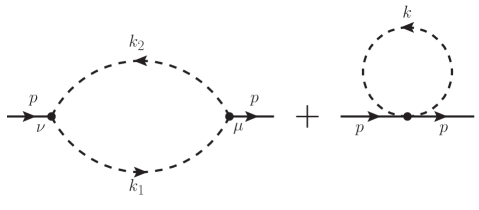
The Feynman diagrams for the self-energy are shown in Fig. (1). The retarded self-energy is
| (39) | |||||
where and denote the vacuum and medium parts respectively. They can be put into the forms (Gale:1990pn, ),
| (40) |
where the transverse and longitudinal projectors are defined as
| (41) |
Here is the flow velocity, in the comoving frame, it becomes . In Eq. (40), , and are given as
| (42) | |||||
| (43) | |||||
| (44) | |||||
where momentum functions and are defined as
| (45) | |||||
| (46) | |||||
| (47) |
In Eqs. (45-47), We have assumed that are in thermal equilibrium, so and are Bose-Einstein distribution depending on the temperature and chemical potential . Here we have written the self-energy in the same forms as in our previous work (Dong:2024nxj, ), and one can prove that it is identical to the results in Ref. (Gale:1990pn, ).
Finally, the total self-energy can be written as
| (48) |
where and are defined as
| (49) |
IV.3 Spectral function
Inserting Eq. (48) into Eq. (36), we can solve as a function of and ,
| (50) |
where we have used
| (51) |
We can read out the longitudinal and transverse spectral function from Eq. (50) as
| (52) |
From the relation (fetter2003quantum, ; zubarev1997statistical, ) ( for ), the leading order Wigner function reads
| (53) |
Here is the Bose-Einstein distribution. Inserting Eq. (53) into Eq. (20), we can obtain the leading order contribution to the spin density matrix.
V Linear Response Theory
In this section, we will derive the NLO correction to the Wigner function by linear response theory. We will use the Kubo formula derived in Zubarev’s approach (Zubarev_1979, ; Hosoya:1983id, ; Becattini:2019dxo, ).
The linear response of an observable for the operator to the perturbation reads (Becattini:2019dxo, )
| (54) | |||||
where is the expectation value in non-equilibrium while is the expectation value in local equilibrium, and are non-equilibrium and local equilibrium density operators respectively, with and being the flow velocity and temperature respectively, and is the energy-momentum tensor for the vector field give by
| (55) |
We choose the operator in Eq. (54) to be the Wigner function operator
| (56) |
The correction to from the perturbation can be written as
| (57) |
where denotes the thermal shear stress tensor, and the tensor is defined as
| (58) | |||||
The detailed derivation of can be found in (Li:2022vmb, ; Dong:2024nxj, ).
Now the total Wigner function is
| (59) |
where the LO and NLO contributions are given by Eqs. (53) and (57) respectively. Inserting Eq. (59) into Eq. (20), the deviation of the spin density matrix from 1/3 can be expressed as
| (60) |
In order to numerically calculate the spin density matrix that can be compared with experimental data in momentum space, we have to integrate over on the freeze-out hypersurface for both numerator and denominator in Eq. (60) as
| (61) |
where is the freeze-out hypersurface. If the system evolves homogeneously in time, is actually the space volume, so . The above formula is the starting point for the numerical calculation in the next section.
VI Numerical Results
In this section, we will numerically calculate and by Eq. (61). The parameters are chosen as 770 MeV, 139 MeV, 6.07 for the coupling constant (Gale:1990pn, ), 150 MeV for the freeze-out temperature. The rapidity range is set to . The freeze-out hypersurface and thermal shear stress tensor are calculated by hydrodynamical model CLVisc at 11.5, 19.6, 27, 39, 62.4 and 200 GeV and 20-50% centrality (Pang:2018zzo, ; Wu:2021fjf, ; Wu:2022mkr, ). Here we assume that the thermal shear stress tensor does not change a lot before and after hadronization, so we can apply it to the system.
VI.1 Results for
From Eq. (61), the LO contribution to involves
| (62) |
We see that the spin alignment as a function of the momentum may be non-vanishing at the LO although the momentum integrated spin alignment at the same order should be zero. The NLO contribution involves
| (63) | |||||
| (64) | |||||
The NLO contribution is proportional to the thermal shear stress tensor , so it may contribute to the momentum integrated spin alignment. It is important to note that the coefficient of increases with increasing , so the expansion will break down for large . In other words, the linear response theory only works for low momenta.
The spin alignment as functions of the transverse momentum and azimuthal angle in the central rapidity is shown in Fig. (2), and as functions of the collision energy is shown in Fig. (3). We can see in Fig. (2a) that (the spin alignment) at the LO is negative for 0.5 GeV and positive for 0.5 GeV but with very small magnitude of the order , while its NLO contribution is negative and its magnitude increases with due to the term proportional to in Eqs. (63-64). It turns out that the total values of from the LO and NLO are negative in the region up to 2 GeV. Note that the non-vanishing values of the LO contribution to are due to the space-time integration on the freezeout hypersurface and the rapidity range. The azimuthal angle dependence of is shown in Fig. (2b) in an oscillation pattern with the magnitude at the LO being about . We see that is positive for and negative for . The NLO contribution to is slightly smaller than zero since it is suppressed by for high in integration. Fig. (3) shows that the LO contribution to is independent of the collision energy, while the NLO contribution is negative and decreases with the collision energy when it is lower than about 50 GeV.


VI.2 Results for
From Eq. (61), the LO and NLO contributions to involve
| (65) | |||||
| (66) | |||||
Here the denominator is the same as in . Similarly, the LO contribution to as a momentum function may be non-vanishing although the momentum integrated one should be vanishing. The NLO contribution may give rise to both integrated and un-integrated non-zero .
The off-diagonal element as functions of and in the central rapidity range is presented in Fig. (4), and its dependence on the collision energy is presented in Fig. (5). In Fig. (4a), we can see that the LO contribution is negative for low and positive for high with the magnitude of the order . The NLO contribution is negative and its magnitude increases with , which is also a result of the term. As shown in Fig. (4b), as functions of has an oscillation pattern similar to but with an opposite sign, due to the different signs of terms in Eqs. (62) and (65) (we can express as ). The collision energy dependence of also has the similar behavior to , as shown in Fig. (5).


In conclusion, the contributions from the spectral function and from the thermal shear stress tensor to the spin density matrix of mesons are of the order of . For un-integrated quantities, and are all negative and decrease with , and and show oscillation patterns but with opposite signs. The momentum integrated and are all negative and decrease with the collision energy when the collision energy is less than about 50 GeV, while they are almost constant when the collision energy is higher.
VII Summary and conclusions
We study the spin density matrix of neutral mesons contributed from the spectral function and thermal shear tensor with the Kubo formula in the linear response theory. We introduce the two-point Green’s function in the CTP formalism which defines the Wigner function and the MVSD in phase space for neutral mesons. As the leading order contribution, the spectral function of the neutral meson can be obtained from the Dyson-Schwinger equation for the retarded Green’s function with and interactions in a thermal pion gas. Then the next-to-leading order contribution from the thermal shear tensor can be calculated through the Kubo formula in the linear response theory. Finally we present numerical results for and which have a dominant effect on the correlator in search for the CME. The numerical results for the thermal shear tensor are needed for evaluating the spin density matrix, which can be calculated by hydrodynamical models. The numerical results give negative values for and as functions of the transverse momentum at the order , while their values as functions of the azimuthal angle show oscillation patterns. The momentum integrated and are all negative and decrease with the collision energy when the collision energy is less than about 50 GeV, while they are almost constant for higher collision energies.
Acknowledgements.
The work is supported in part by the National Natural Science Foundation of China (NSFC) under Grant No. 12135011.References
- (1) S. Barnett, Rev. Mod. Phys. 7, 129 (1935).
- (2) A. Einstein and W. de Haas, Deutsche Physikalische Gesellschaft, Verhandlungen 17, 152 (1915).
- (3) Z.-T. Liang and X.-N. Wang, Phys. Rev. Lett. 94, 102301 (2005), nucl-th/0410079, [Erratum: Phys.Rev.Lett. 96, 039901 (2006)].
- (4) S. A. Voloshin, (2004), nucl-th/0410089.
- (5) Z.-T. Liang and X.-N. Wang, Phys. Lett. B 629, 20 (2005), nucl-th/0411101.
- (6) B. Betz, M. Gyulassy, and G. Torrieri, Phys. Rev. C76, 044901 (2007), 0708.0035.
- (7) J.-H. Gao et al., Phys. Rev. C77, 044902 (2008), 0710.2943.
- (8) F. Becattini, F. Piccinini, and J. Rizzo, Phys. Rev. C77, 024906 (2008), 0711.1253.
- (9) STAR, L. Adamczyk et al., Nature 548, 62 (2017), 1701.06657.
- (10) STAR, J. Adam et al., Phys. Rev. C 98, 014910 (2018), 1805.04400.
- (11) HADES, R. Abou Yassine et al., Phys. Lett. B 835, 137506 (2022), 2207.05160.
- (12) ALICE, S. Acharya et al., Phys. Rev. Lett. 128, 172005 (2022), 2107.11183.
- (13) I. Karpenko and F. Becattini, Eur. Phys. J. C 77, 213 (2017), 1610.04717.
- (14) H. Li, L.-G. Pang, Q. Wang, and X.-L. Xia, Phys. Rev. C 96, 054908 (2017), 1704.01507.
- (15) Y. Xie, D. Wang, and L. P. Csernai, Phys. Rev. C 95, 031901 (2017), 1703.03770.
- (16) Y. Sun and C. M. Ko, Phys. Rev. C 96, 024906 (2017), 1706.09467.
- (17) M. Baznat, K. Gudima, A. Sorin, and O. Teryaev, Phys. Rev. C 97, 041902 (2018), 1701.00923.
- (18) S. Shi, K. Li, and J. Liao, Phys. Lett. B 788, 409 (2019), 1712.00878.
- (19) D.-X. Wei, W.-T. Deng, and X.-G. Huang, Phys. Rev. C 99, 014905 (2019), 1810.00151.
- (20) B. Fu, K. Xu, X.-G. Huang, and H. Song, Phys. Rev. C 103, 024903 (2021), 2011.03740.
- (21) S. Ryu, V. Jupic, and C. Shen, Phys. Rev. C 104, 054908 (2021), 2106.08125.
- (22) X.-G. Deng, X.-G. Huang, and Y.-G. Ma, (2021), 2109.09956.
- (23) X.-Y. Wu, C. Yi, G.-Y. Qin, and S. Pu, Phys. Rev. C 105, 064909 (2022), 2204.02218.
- (24) Q. Wang, Nucl. Phys. A967, 225 (2017), 1704.04022.
- (25) W. Florkowski, A. Kumar, and R. Ryblewski, Prog. Part. Nucl. Phys. 108, 103709 (2019), 1811.04409.
- (26) X.-G. Huang, J. Liao, Q. Wang, and X.-L. Xia, (2020), 2010.08937.
- (27) J.-H. Gao, Z.-T. Liang, Q. Wang, and X.-N. Wang, Lect. Notes Phys. 987, 195 (2021), 2009.04803.
- (28) J.-H. Gao, G.-L. Ma, S. Pu, and Q. Wang, Nucl. Sci. Tech. 31, 90 (2020), 2005.10432.
- (29) Y.-C. Liu and X.-G. Huang, Nucl. Sci. Tech. 31, 56 (2020), 2003.12482.
- (30) F. Becattini, Rept. Prog. Phys. 85, 122301 (2022), 2204.01144.
- (31) Y. Hidaka, S. Pu, Q. Wang, and D.-L. Yang, Prog. Part. Nucl. Phys. 127, 103989 (2022), 2201.07644.
- (32) F. Becattini et al., Int. J. Mod. Phys. E 33, 2430006 (2024), 2402.04540.
- (33) G. Bunce et al., Phys. Rev. Lett. 36, 1113 (1976).
- (34) K. Schilling, P. Seyboth, and G. E. Wolf, Nucl. Phys. B 15, 397 (1970), [Erratum: Nucl.Phys.B 18, 332 (1970)].
- (35) Y.-G. Yang, R.-H. Fang, Q. Wang, and X.-N. Wang, Phys. Rev. C 97, 034917 (2018), 1711.06008.
- (36) A. H. Tang et al., Phys. Rev. C 98, 044907 (2018), 1803.05777, [Erratum: Phys.Rev.C 107, 039901 (2023)].
- (37) STAR, M. S. Abdallah et al., Nature 614, 244 (2023), 2204.02302.
- (38) X.-L. Xia, H. Li, X.-G. Huang, and H. Zhong Huang, Phys. Lett. B 817, 136325 (2021), 2010.01474.
- (39) J.-H. Gao, Phys. Rev. D 104, 076016 (2021), 2105.08293.
- (40) B. Müller and D.-L. Yang, Phys. Rev. D 105, L011901 (2022), 2110.15630.
- (41) A. Kumar, B. Müller, and D.-L. Yang, Phys. Rev. D 108, 016020 (2023), 2304.04181.
- (42) X.-L. Sheng, L. Oliva, and Q. Wang, Phys. Rev. D 101, 096005 (2020), 1910.13684, [Erratum: Phys.Rev.D 105, 099903 (2022)].
- (43) X.-L. Sheng, Q. Wang, and X.-N. Wang, Phys. Rev. D 102, 056013 (2020), 2007.05106.
- (44) X.-L. Sheng, L. Oliva, Z.-T. Liang, Q. Wang, and X.-N. Wang, (2022), 2206.05868.
- (45) X.-L. Sheng, L. Oliva, Z.-T. Liang, Q. Wang, and X.-N. Wang, Phys. Rev. Lett. 131, 042304 (2023), 2205.15689.
- (46) X.-L. Sheng, S. Pu, and Q. Wang, Phys. Rev. C 108, 054902 (2023), 2308.14038.
- (47) J. Chen, Z.-T. Liang, Y.-G. Ma, and Q. Wang, Sci. Bull. 68, 874 (2023), 2305.09114.
- (48) X.-L. Sheng, Z.-T. Liang, and Q. Wang, Acta Phys. Sin. (in Chinese) 72, 072502 (2023).
- (49) J. Chen et al., Nucl. Phys. News 34, 17 (2024).
- (50) J.-H. Chen, Z.-T. Liang, Y.-G. Ma, X.-L. Sheng, and Q. Wang, Sci. China Phys. Mech. Astron. 68, 211001 (2025), 2407.06480.
- (51) F. Li and S. Y. F. Liu, (2022), 2206.11890.
- (52) W.-B. Dong, X.-L. Sheng, Y.-L. Yin, and Q. Wang, Global polarization and spin alignment in heavy-ion collisions: past, present and future, in 25th International Spin Symposium, 2024, 2401.15576.
- (53) D. Kharzeev, Phys. Lett. B 633, 260 (2006), hep-ph/0406125.
- (54) D. E. Kharzeev, L. D. McLerran, and H. J. Warringa, Nucl. Phys. A 803, 227 (2008), 0711.0950.
- (55) K. Fukushima, D. E. Kharzeev, and H. J. Warringa, Phys. Rev. D 78, 074033 (2008), 0808.3382.
- (56) S. A. Voloshin, Phys. Rev. C 70, 057901 (2004), hep-ph/0406311.
- (57) STAR, L. Adamczyk et al., Phys. Rev. C 88, 064911 (2013), 1302.3802.
- (58) STAR, L. Adamczyk et al., Phys. Rev. C 89, 044908 (2014), 1303.0901.
- (59) F. Wang and J. Zhao, Phys. Rev. C 95, 051901 (2017), 1608.06610.
- (60) A. H. Tang, Chin. Phys. C 44, 054101 (2020), 1903.04622.
- (61) D. Shen, J. Chen, A. Tang, and G. Wang, Phys. Lett. B 839, 137777 (2023), 2212.03056.
- (62) Y.-L. Yin, W.-B. Dong, J.-Y. Pang, S. Pu, and Q. Wang, (2024), 2402.03672.
- (63) D. N. Zubarev, A. V. Prozorkevich, and S. A. Smolyanskii, Theoretical and Mathematical Physics 40, 821 (1979).
- (64) A. Hosoya, M.-a. Sakagami, and M. Takao, Annals Phys. 154, 229 (1984).
- (65) F. Becattini, M. Buzzegoli, and E. Grossi, Particles 2, 197 (2019), 1902.01089.
- (66) C. Gale and J. I. Kapusta, Nucl. Phys. B 357, 65 (1991).
- (67) L.-G. Pang, H. Petersen, and X.-N. Wang, Phys. Rev. C 97, 064918 (2018), 1802.04449.
- (68) X.-Y. Wu, G.-Y. Qin, L.-G. Pang, and X.-N. Wang, Phys. Rev. C 105, 034909 (2022), 2107.04949.
- (69) P. C. Martin and J. S. Schwinger, Phys. Rev. 115, 1342 (1959).
- (70) L. V. Keldysh, Zh. Eksp. Teor. Fiz. 47, 1515 (1964).
- (71) K.-c. Chou, Z.-b. Su, B.-l. Hao, and L. Yu, Phys. Rept. 118, 1 (1985).
- (72) J.-P. Blaizot and E. Iancu, Phys. Rept. 359, 355 (2002), hep-ph/0101103.
- (73) Q. Wang, K. Redlich, H. Stoecker, and W. Greiner, Phys. Rev. Lett. 88, 132303 (2002), nucl-th/0111040.
- (74) J. Berges, AIP Conf. Proc. 739, 3 (2004), hep-ph/0409233.
- (75) W. Cassing, Eur. Phys. J. ST 168, 3 (2009), 0808.0715.
- (76) M. Crossley, P. Glorioso, and H. Liu, JHEP 09, 095 (2017), 1511.03646.
- (77) W.-B. Dong, Y.-L. Yin, X.-L. Sheng, S.-Z. Yang, and Q. Wang, Phys. Rev. D 109, 056025 (2024), 2311.18400.
- (78) D. Wagner, N. Weickgenannt, and E. Speranza, (2023), 2306.05936.
- (79) A. Fetter and J. Walecka, Quantum Theory of Many-particle SystemsDover Books on Physics (Dover Publications, 2003).
- (80) D. Zubarev, V. Morozov, and G. Röpke, Statistical Mechanics of Nonequilibrium Processes, Statistical Mechanics of Nonequilibrium Processes. Volume 2: Relaxation and Hydrodynamic ProcessesStatistical Mechanics of Nonequilibrium Processes (Wiley, 1997).