Spin-Spin Correlations in the Kitaev Model at Finite Temperatures: Approximate and Exact Results via Green’s Function Equation of Motion

Quantum spin liquids have emerged as a central topic in condensed matter physics, capturing significant attention due to their complex and intriguing properties Savary and Balents (2017). Among the various theoretical models, the Kitaev model is particularly notable for its exactly solvable ground state, which features fractionalized Majorana fermions Kitaev (2006). This model is not only analytically tractable but also holds potential for real-world applications in materials with significant spin-orbit coupling Jackeli and Khaliullin (2009); Takagi et al. (2019). Majorana fermions play a crucial role in the development of topological quantum computers, offering a platform for fault-tolerant quantum computation Kitaev (2003); Nayak et al. (2008).

While investigating the Kitaev model in terms of Majorana fermions provides significant mathematical elegance, a deeper understanding of the physical nature of Majorana fermions may be achieved through the study of spin operators. However, the Kitaev model presents substantial challenges due to its highly frustrated and strongly correlated nature.

In this paper, we employ the spin Green’s function approach for the spin operators while preserving SU(2) symmetry and solve its equation of motion. This method, which maintains SU(2) symmetry Kondo and Yamaji (1972), is particularly suitable because the system does not exhibit magnetic long-range order even at zero temperature. Another critical observation is that the spin-spin correlation function in the ground state is finite only between nearest neighbor sites Baskaran et al. (2007), suggesting that the spin-spin correlation length remains short-ranged even at finite temperatures. Since the equation of motion for the Green’s function Zubarev (1960) relies on finite-range correlation functions, it is well-suited for exploring the finite temperature properties of the Kitaev model. Additionally, this approach aligns with the high-temperature expansion Kondo and Yamaji (1972), enhancing the accuracy of results at higher temperatures. Physically, our spin Green’s function describes the propagation of a pair of $\mathbb{Z}_{2}$ fluxes. Our results demonstrate that the computed temperature dependence of the correlation functions yields a value at zero temperature that is quite close to the exact value. Furthermore, we present several exact results regarding spin-spin correlation functions at finite temperatures.

The Hamiltonian of the isotropic Kitaev model on the honeycomb lattice is given by Kitaev (2006):

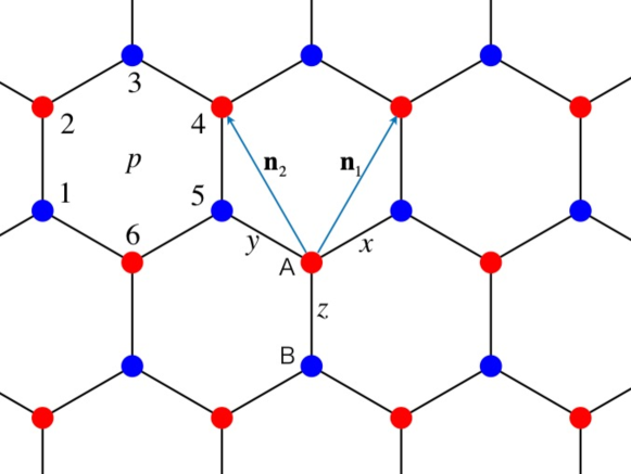
where $S_{i}^{\gamma}$ is the $\gamma$-component of the spin-1/2 operator at site $i$, and we consider the ferromagnetic Kitaev coupling $K>0$. The summation of ${\langle i,j\rangle}_{\gamma}$ represents the sum over the nearest neighbor sites connected by a $\gamma$ bond, as shown in Fig. 1. In the honeycomb lattice, each unit cell comprises two sites corresponding to the A and B sublattices, as illustrated in Fig. 1. Additionally, Fig. 1 shows a plaquette $p$ consisting of six sites. For this plaquette, we define the following plaquette operator Kitaev (2006):

where $\sigma_{i}^{\gamma}$ represents the $\gamma$-component of the Pauli matrix at site $i$. $\sigma_{i}^{\gamma}$ can be expressed as $\sigma_{i}^{\gamma}=ib_{i}^{\gamma}c_{i}$ in terms of two types of Majorana fermions Kitaev (2006), where this equality holds by restricting the extended Hilbert space of Majorana fermions to the physical Hilbert space of the original spin operators. The product of two Majorana fermions, $b_{i}^{\gamma}$ and $b_{j}^{\gamma}$, residing at nearest neighbor sites forms a $\mathbb{Z}_{2}$ gauge field. In this formulation, $W_{p}$ represents the $\mathbb{Z}_{2}$ gauge flux. Meanwhile, the Majorana fermions $c_{i}$ are itinerant under these $\mathbb{Z}_{2}$ gauge fields.

An intriguing aspect of the Kitaev model is that it has been rigorously demonstrated that its ground state is a spin liquid state without long-range magnetic order. Because of the absence of the magnetic long-range order, we may apply SU(2) invariant formalsim of the Green’s function methodKondo and Yamaji (1972). We define the Matsubara Green’s function:

Here $\tau$ represents the imaginary time and $T_{\tau}$ represents the imaginary time ordering operator. The notation $S_{n{\alpha}}^{\gamma}$ represents the $\gamma$-th component of the spin operator for the $\alpha$-th sublattice within the $n$-th unit cell.

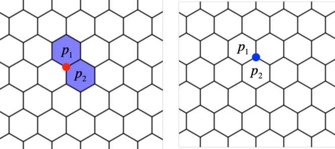
Before delving into the analysis of the Green’s function, we first discuss its physical meaning. Specifically, we consider the Green’s function (3) with $\gamma=x$, $\alpha_{1}=B$, and $\alpha_{2}=A$. This Green’s function describes a process where the $\mathbb{Z}_{2}$ flux values at adjacent hexagon plaquettes are flipped at imaginary time $0$ and then flipped again at imaginary time $\tau$. This process is schematically illustrated in Fig. 2. We observe that any flipped $\mathbb{Z}_{2}$ flux values must be flipped again; otherwise, the thermal average will vanish.

Denoting the inverse temperature by $\beta=1/T$, where $T$ is the temperature, and setting the Boltzmann constant $k_{\rm B}$ to 1, the Fourier representation of Eq. (3) in the Matsubara frequency, $\omega_{n}=2\pi n/\beta$ with $n$ being an integer, is given by

To find the expression for the Green’s function, we first take the derivative of Eq. (3) with respect to $\tau$ and then perform the Fourier transform. This process yields

Now we have a new Green’s function, represented by the first term on the right-hand side. The equation of motion for this Green’s function is given by

We first compute $\left[{{\cal H},S_{n{\alpha 1}}^{\gamma}}\right]$, and then compute $\left[{{\cal H},\left[{{\cal H},S_{n{\alpha_{1}}}^{\gamma}}\right]}\right]$. From the latter calculation, terms like ${\left\langle{{S_{nA}^{\gamma}S_{{n_{1}}B}^{x}S_{{n_{2}}A}^{\gamma}}}\mathrel{\left|{\vphantom{{S_{nA}^{\gamma}S_{{n_{1}}B}^{x}S_{{n_{2}}A}^{\gamma}}{S_{m\alpha}^{x}}}}\right.\kern-1.2pt}{{S_{m\alpha}^{x}}}\right\rangle_{i{\omega_{n}}}}$, ${\left\langle{{S_{n}^{\gamma}S_{{n_{1}}B}^{\gamma}S_{{n_{2}}A}^{x}}}\mathrel{\left|{\vphantom{{S_{n}^{\gamma}S_{{n_{1}}B}^{\gamma}S_{{n_{2}}A}^{x}}{S_{m\alpha}^{x}}}}\right.\kern-1.2pt}{{S_{m\alpha}^{x}}}\right\rangle_{i{\omega_{n}}}}$, etc., appear. Instead of considering the equation of motion for such terms, we approximate them as the product of a correlation function and a Green’s function with a reduced number of spins, using the so-called Tyablikov decoupling Tyablikov and Bonch-Bruevich (1962), as follows:

where $\alpha$ is a correction parameter in this approximationKondo and Yamaji (1972) to be determined from the constraint. The approximation is more accurate when one applies this decoupling scheme at Green’s functions with more spins or in higher spatial dimensionsSasamoto and Morinari (2024). Here, the correlation functions are defined by

with ${\bf R}_{n}$ being the coordinate vector of the $n$-th unit cell.

After a tedious but straightforward calculation followed by a Fourier transform to momentum space, we obtain

The matrix form of the Green’s function, ${{G}^{x}}\left({{\bf{q}},i{\omega_{n}}}\right)$, is given by:

The components of the matrices $M({\bf q})$ and $N({\bf q})$ are:

and

respectively. We obtain a similar formula for ${{G}^{y}}\left({{\bf{q}},i{\omega_{n}}}\right)$ and ${{G}^{z}}\left({{\bf{q}},i{\omega_{n}}}\right)$. However, due to the symmetry of the honeycomb lattice, we do not need these for the isotropic case.

Solving Eq. (10), we obtain

The energy dispersion $\omega_{\bf{q}}^{(\pm)}$ is given by

with ${\lambda_{\bf{q}}}=\sqrt{{{\left|{{b_{\bf{q}}}}\right|}^{2}}-{{\left|{{\mathop{\rm Im}\nolimits}{a_{\bf{q}}}}\right|}^{2}}}$. The terms $a_{\bf q}$ and $b_{\bf q}$ are defined by

In our Green’s function approach, we determine the correlation functions in a self-consistent manner. The correlation functions are expressed in terms of the Green’s function as

where $N$ is the number of unit cells. In the numerical calculations below, we take $N=45\times 45$. There are relationships between the correlation functions due to the absence of magnetic long-range order and any symmetry breaking. By utilizing these symmetries, we define

The self-consistent equations to be solved are then given by

where $g(x)=x\coth x$. The last equation is obtained from $c_{AA}^{x}\left(0\right)=1/4$. $Z_{AA}^{\pm}$ and $Z_{AB}^{\pm}$ are given by

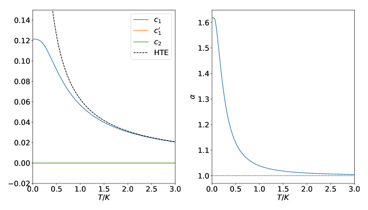
The temperature dependencies of $c_{1}$, $c^{\prime}_{1}$, and $c_{2}$ are shown in the left panel of Fig. 3. The value of $4c_{1}$ converges to 0.4859 as $T$ approaches zero, closely approximating the exact valueBaskaran et al. (2007) of $0.5249\equiv 4c_{1}^{\rm exact}$. At high temperatures, the behavior of $c_{1}$ aligns well with the high-temperature expansion result, expressed as $c_{1}=\beta K/16+O(\beta^{3})$. Meanwhile, $c^{\prime}_{1}$ and $c_{2}$ remain zero across all temperatures, a finding rigorously confirmedBaskaran et al. (2007) at $T=0$ and consistent even at finite temperatures. The vanishing of $c^{\prime}_{1}$ and $c_{2}$ can be understood as follows. Consider, for instance, $c_{AB}^{x}(0)=\left\langle S_{0A}^{x}S_{0B}^{x}\right\rangle$, which corresponds to $c^{\prime}_{1}$. In this correlation function, the spin operator $S_{0B}^{x}$ flips the $\mathbb{Z}_{2}$ flux values of the adjacent hexagons that share the $x$-bond emanating from the B sublattice in the 0-th unit cell. Similarly, the spin operator $S_{0A}^{x}$ flips the $\mathbb{Z}_{2}$ flux values of the adjacent hexagons that share the $x$-bond emanating from the A sublattice in the 0-th unit cell. Since the hexagons affected by $S_{0B}^{x}$ and $S_{0A}^{x}$ are different and the Hamiltonian $H$ does not alter the $\mathbb{Z}_{2}$ flux values, the thermal average of their product is identically zero. This reasoning also applies to the other correlation functions, highlighting a unique characteristic of the Kitaev model. The same argument leads to $\left\langle{{T_{\tau}}S_{n{\alpha_{1}}}^{\gamma_{1}}\left(\tau\right)S_{m{\alpha_{2}}}^{\gamma_{2}}\left(0\right)}\right\rangle\equiv 0$ for $\gamma_{1}\neq\gamma_{2}$. The flux values flipped by $S_{m{\alpha_{2}}}^{\gamma_{2}}$ at imaginary time 0 cannot be flipped again by $S_{n{\alpha_{1}}}^{\gamma_{1}}$ at imaginary time $\tau$. We note that this result is exact. From this observation, we may restrict the two-spin Green’s function to the form of Eq. (3). We also note that the vanishing of $c^{\prime}_{1}$ and $c_{2}$ results in $\omega_{\bf{q}}^{\pm}$ forming a flat band, given by $K\sqrt{\left(1\pm 4\alpha{c_{1}}\right)/2}$.

In the right panel of Fig. 3, we present the temperature dependence of $\alpha$. As temperature increases, $\alpha$ approaches one, indicating that the decoupling approximation in Eqs. (7) and (8) becomes exact without the need for the correction parameter $\alpha$. However, deviations of $\alpha$ from one at lower temperatures suggest the necessity of this correction parameter in the equations.

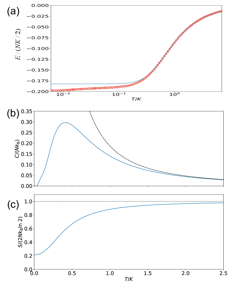
From the temperature dependence of $c_{1}$, the internal energy can be computed using the relation

We compared the temperature dependence of the energy with the results shown in Fig. 15(a) of Ref. Motome and Nasu, 2020, as shown in Fig. 4(a). We found an almost perfect match for $T>T_{H}$ with $T_{H}\simeq 0.375K$, but our energy values are slightly higher for $T<T_{H}$. This discrepancy likely originates from the error in the $c_{1}$ value at $T=0$. Although the relative error is $|(c_{1}^{\rm exact}-c_{1})/c_{1}^{\rm exact}|\simeq 0.07$, minor details and significant physics, such as the fractionalization of spins, may be hidden within this discrepancy.

Figure 4 shows the temperature dependencies of the specific heat and entropy. The specific heat is calculated from the temperature derivative of the internal energy $E$ and compared with the high-temperature expansion (HTE) result, $C_{\rm HTE}=3NK^{2}\beta^{2}/16$. The entropy is computed using the formula:

where $S\left(\infty\right)=2N\ln 2$ and $T_{0}$ is a sufficiently large value at which the Green’s function result for the specific heat closely approximates the HTE result (here, we take $T_{0}/K=10$). The specific heat exhibits a single broad peak around $T/K\simeq 0.4$, consistent with mean field calculations Saheli et al. (2024). We likely fail to observe the low-temperature peak around $T_{L}\simeq 0.012K$ reported in Ref. Nasu et al., 2015 due to the discrepancy mentioned above. The entropy indicates the presence of residual entropy, but if fractionalization were captured, this residual entropy should vanish, as it has been rigorously shown that there are no $\mathbb{Z}_{2}$ fluxes in the ground state and the system must satisfy the third law of thermodynamics.

In conclusion, we have investigated the Kitaev model at finite temperatures using a Green’s function approach that maintains SU(2) symmetry. Our computations of the temperature dependence of the correlation functions revealed that the nearest neighbor spin-spin correlation functions closely match the exact values at zero temperature. Additionally, we have presented several exact results concerning the spin Green’s function and spin-spin correlation functions specific to the Kitaev model. These findings enhance our understanding of the Kitaev model and provide a novel approach to this model without relying on Majorana fermions. This work opens up new avenues for exploring the dynamic properties of the Kitaev model and its applications in the study of quantum spin liquids and topological quantum computing.