metrics of cohomogeneity one with Aloff–Wallach spaces as principal orbits
Abstract
In this article, we construct two continuous 1-parameter family of non-compact metrics with both chiralities, with the principal orbit an Aloff–Wallach space and the singular orbit . For a generic , metrics constructed are locally asymptotically conical (ALC). For , we construct two continuous 1-parameter families with geometric transition from asymptotically conical (AC) metrics to ALC metrics.
1 Introduction
Metrics with holonomy are interesting subjects in differential geometry and theoretical physics. The first example was constructed in [Bry87] on the cone over Berger space . The first complete example was constructed in [BS89] and [GPP90] on the spinor bundle over . The first compact example was constructed in [Joy96]. In recent years, metrics with an Aloff–Wallach space as principal orbit became an active field of research. It is expected that a cohomogeneity one space with an Aloff–Wallach space as its principal orbit admits a continuous 1-parameter family of metrics with asymptotically locally conical (ALC) asymptotics: each metric’s asymptotic limit is a product between a 7-dimensional Ricci-flat cone and a circle with fixed radius . Moreover, with , the metric converges to an asymptotically conical (AC) one: its asymptotic limit is an 8-dimensional cone. In this way, one has a continuous 1-parameter family of metrics with non-maximal volume growth and its boundary is a metric with maximal volume growth.
An Aloff–Wallach space is a homogeneous space , where is embedded in as with integers and . Without loss of generality, we assume that and are coprime. Using outer automorphism and Weyl group of to normalize , we assume in this article. Due to the geometric differences, we call an exceptional Aloff–Wallach space if and a generic Aloff–Wallach space if otherwise. With an Aloff–Wallach space as the principal orbit, one can reduce the Einstein equations to a system of nonlinear second order ODEs. The condition, being Ricci-flat, is reduced to a system of first order ODEs. The isolated explicit solution of cohomogeneity one metric with as principal orbit and as singular orbit was given in [GS02]. In [Rei11], the author proved that singular orbit of a cohomogeneity one metric with a fixed can only be either or . The singular orbit appears exclusively for the case . Recently, some ALC metrics with as principal orbit and as singular orbit were constructed in [Fos21]. The setting with as the principal orbit was further studied in [Leh20], in which examples in [GS02] and [Fos21] were extended to two continuous families of ALC metrics. The boundary of each family is an AC metric. Explicit solutions with as principal orbit were given in [CGLP01] and [KY02a]. In [Baz07] and [Baz08], it is observed that formulas for condition in [CGLP02a] and [CGLP02b] can be applied in a broader setting where the cohomogeneity one manifold is deformed from a HyperKähler cone. Specifically, by using the 3-Sasakian structure on , a 2-parameter family of metrics was constructed on a complex line bundle over in [Baz07] and a 2-parameter family of metrics was constructed on a quaternionic line bundle over in [Baz08]. Explicit isolated solutions with a generic as principal orbit are included in [KY02a] and[CGLP02a].
This article aims to prove the global existence of two continuous 1-parameter families of metrics of cohomogeneity one with any Aloff–Walach spaces as principal orbit. Past examples mentioned above are partially recovered in the construction. Specifically, a fixed can be viewed as fiber bundles over with lens spaces , and as fibers, respectively. Let and , define to be the bundle over with as principal orbit. We prove the following theorems.
Theorem 1.1.
Let be coprime. Let . If is generic, there exists a continuous 1-parameter family of forward complete metrics on . metrics on and the ones on have opposite chirality. All ’s and ’s have ALC asymptotics with space at infinity as an bundle over the cone over the nearly-Kähler .
Note that for a generic as the principal orbit, metrics on do not include the explicit ALC metrics in [CGLP02a] and [KY02a]. Hence it is likely to extend the continuous family of ALC metrics in Theorem 1.1 to a larger family using other methods. Metrics on are new to the best knowledge of the author.
It is worth mentioning that our method for proving Theorem 1.1 also applies for the case of exceptional . Only ALC metrics are constructed in this way. For each , the obtained metrics with both chiralities on can be identified by a global symmetry. They are part of the results obtained in [Leh20]. They have smooth extension to the singular orbit . For a more complete study on the metrics with as principal orbit, please see [Fos21] and [Leh20] for more details.
We also consider the case where the principal orbit is the exceptional
Theorem 1.2.
There exists a continuous 1-parameter family of forward complete metrics on with and . metrics on and the ones on have opposite chiralities. All ’s and ’s have an ALC asymptotics with space at infinity as an bundle over the cone over the nearly-Kähler if . If , then the metrics have AC asymptotics with tangent cones at infinity with base homogeneous Einstein metrics on .
Metrics on the orbifold are the ALC metrics in [CGLP01] and some of the solutions in [Baz07]. It is worth mentioning that is in fact . Metrics on are the ones that were conjectured in [KY02b]. For most of the cases, we do not have metrics that shows geometric transition from AC metrics to ALC metrics like the ones that occur in [CGLP02a] and [Leh20]. However, if the principal orbit is , we do have two continuous 1-parameter families of metrics that have metrics on their respective boundaries. In particular, the AC metric on is the Calabi HyperKähler metric in [Cal79]. In other words, the 1-parameter family of ALC metrics on can be desingularized with Calabi’s AC metric.
This article is structured as the following. In Section 2, we study the Ricci-flat system with an as the principal orbit and apply coordinate change that is similar to the one in [Chi19b] and [Chi21]. The coordinate change transforms the singular orbit , the AC asymptotics, and the ALC asymptotics to critical points of a polynomial system. The singular orbit , uniquely appears in the case, is blown up to the infinity in the new coordinate. Although being more complicated than the subsystem, the Ricci-flat system has some important estimate that is not obvious in the subsystem.
In Section 3, we study critical points of the subsystem and recover the locally existing result in [Rei11]. The cohomogeneity one metrics are represented by integral curves that emanates from various critical points.
In Section 4, we prove the global existence and the asymptotic limit by constructing compact invariant sets. The construction boils down to a classical algebraic geometry problem, which requires one to show non-negativity of a resultant polynomial. For readability, the very technical computation and formula are presented in the Appendix.
Acknowledgements. The author would like to thank NSFC for partial support under grants No. 11521101 and NO. 12071489. Thanks also go to Michael Baker, Jesse Madnick and McKenzie Wang for useful discussions.
2 The holonomy cohomogeneity one system
In this section, we study the cohomogeneity one Ricci-flat system on derived in [Rei11]. We apply a coordinate change so that the system becomes a system of first order polynomial ODEs. The condition, originally a first order subsystem, is then transformed to a set of algebraic equation in the new coordinate.
Consider an Aloff–Wallach space , we fix the basis for as the one in [Rei11]. Specifically, we work with the basis
| (2.1) |
where generates . The isotropy representation is decomposed as
where
Recall our convention of Aloff–Wallach spaces, we set and to be coprime and without loss of generality. Under this setting, if is generic, i.e., , one can conclude that all ’s are non-trivial and have different weights. The isotropy representation then consists of 4 inequivalent irreducible summands. The group action of on (2.1) generates a frame for an -invariant Einstein metric . The matrix representation of is hence
| (2.2) |
for some . Consider the cohomogeneity one metric , where each component in (2.2) is a function of . Methods in [EW00] can be applied to derive the cohomogeneity one Einstein system. Let . As shown in [Rei11], the cohomogeneity one Ricci-flat system is
| (2.3) |
with conservation law
| (2.4) |
The conserved quantity (2.4) is essentially equivalent to having zero scalar curvature. Note that the RHS of (2.4) is the scalar curvature of .
If , then by our convention, we either have or . In the first case, there are two equivalent isotropy summands in . In the latter case, the isotropy representation consists of three trivial representations and two equivalent isotropy summands . Therefore, invariant metrics on and are not necessarily diagonal.
For , the matrix representation of an -invariant is
| (2.5) |
From [Rei08] we learn that . One can further reduce the number of functions from 6 to 5, since the residual action of on changes and while leaving diagonal entries unchanged. The metric is invariant if and only if its diagonal. In other words, with the enhanced symmetry, the dynamic system is simply and with
For , the matrix representation of an -invariant is
| (2.6) |
The normalizer is isomorphic to and . The residual action of acts as on the three trivial representations [Rei08]. Therefore, one can use the to partially diagonalize so that all ’s vanish and the number of functions is reduced from 10 to 7. A -invariant may still not be diagonal. Nevertheless, one can consider the case with diagonal , as shown in in [Rei11]. In this article, we further impose the condition and study (2.3) and (2.4) with . One can check that such a dynamic system is a subsystem of in [Rei11]. For the case where and are unequal, please see [Baz07] for more details.
Singular orbits of cohomogeneity one space , and are generated by , and , respectively. Hence according to [EW00] for the case and the power series in [Rei11] for the rest of the orbifolds, the initial conditions for theses three types of bundles, are respectively given by
| (2.7) |
For exceptional Aloff–Wallach spaces, recent development in [VZ20] can also be applied to derive the initial condition even with equivalent isotropy summands.
The condition is derived in [Rei11] as the following
| (2.8) |
Change the sign of in (2.8). We then obtain the condition with the opposite chirality:
| (2.9) |
Although we mainly consider the construction of metrics in this article, we start with the Ricci-flat system. As shown in the following, with a coordinate change, some important estimates can be quickly derived from the new Ricci-flat system while it is not obvious in the new subsystem.
It is clear that
is the second fundamental form of in at time . The quantity in (2.3) is hence the mean curvature. In many works on the construction of cohomogeneity one Einstein metrics, the coordinate change can help to simplify the original Einstein system[DW09][BDW15][Chi19a]. This case is no exception. Define functions
| (2.10) |
And define functions
| (2.11) |
Use ′ to denote the derivative with respect to . (2.3) is transformed to
| (2.12) |
The conservation law (2.4) becomes
| (2.13) |
Note that . Therefore, can be treated as function of by
To recover the original coordinate, we simply compute
and
From the definition of ’s in (2.10), one expects is preserved by the new dynamic system. Indeed, since
| (2.14) |
it is clear that
is invariant. It is worth mentioning that in many works on constructing cohomogeneity one steady Ricci solitons[DW09][BDW15][Win17], coordinate change is applied, where is the potential function. For our case, one obtains the same polynomial system as (2.12) with
where the equality is needed for (2.14) to hold. From this perspective, one can treat the invariance of as the outcome of setting the potential of cohomogeneity one steady Ricci solitons to be a constant. From (2.12), it is clear that we can assume ’s be non-negative without loss of generality. In fact, the set is invariant. A straightforward observation also gives the following proposition.
Proposition 2.1.
The set is invariant.
Proof.
It is clear that
| (2.15) |
If non-transverse crossings emerge on an integral curve, then in addition to at the crossing point, either for distinct or at that point. Then such an integral curve must lie in either the invariant set or and the condition is held along the integral curve. Hence we exclude the possibility of non-transverse crossings. The proof is complete. ∎
Therefore, cohomogeneity one Ricci-flat metrics with an Aloff–Wallach space as the principal orbit is represented by an integral curve to (2.12) on the following subset of :
| (2.16) |
a -dimensional algebraic surface with boundary. By Lemma 5.1 in [BDW15], we know that . Therefore, if an integral curve is defined on , then the Ricci-flat metric represented is forward complete.
We now consider the condition (2.8) and (2.9) in the new coordinate. The condition form an invariant subset of with a lower dimension. Specifically, (2.8) turns to
| (2.17) |
It is known that metrics are Ricci-flat. Hence (2.8) is a first order subsystem of (2.3). This is can also be shown using the new coordinates. Define . We claim the following.
Proposition 2.2.
is invariant.
Proof.
Replace ’s in (2.13), we obtain
On the other hand, on , we have
| (2.19) |
Therefore, can also be expressed as the intersection
| (2.20) |
Cohomogeneity one metrics with an Aloff–Wallach space as the principal orbit is represented by an integral curve to (2.12) restricted on , a 3-dimensional algebraic surface in with boundaries. In other words, the metrics can be represented by integral curves to the vector field that consists of the last four entries of , where ’s are polynomials defined as in (2.17). Such a dynamic system has a conservation law given by (2.19).
For the condition with the opposite chirality, (2.9) becomes
| (2.21) |
which is also a subsystem of (2.12). Define to be
| (2.22) |
With the similar computation as the one in Proposition 2.2, we can also show that is invariant.
Remark 2.3.
Proposition 2.4.
On , we have .
Proof.
Summing all equations in (2.17), we obtain
| (2.23) |
Hence in . Similar argument can prove the statement for . ∎
There exists an invariant subset that lies in both and . Define
| (2.24) |
Equivalently, we have . It is clear that is a 2-dimensional invariant set. System (2.12) restricted on is essentially the system for cohomogeneity one metric with as singular orbit and as principal orbit. For a forward complete ALC Ricci-flat metric, components and in (2.2) increase linearly and converges to a constant as . The integral curve that represents such a metric converges to the invariant set as . Therefore, one can also think of as a subset of the “space of ALC asymptotics”. Such an invariant subset also occurs in the dynamic system in [Chi21]. By [CS02], all integral curves on are explicitly known. More details are discussed in Section 4.4.
3 Local Existence
In this section, we compute linearizations of some important critical points of (2.12). In particular, we compute linearization at some critical points that are in and recover the local existence of metrics on the tubular neighborhood around as in [Rei11].
Critical points of (2.12) on are the following.
-
I
.
These critical points represent the initial conditions (2.7) in the new coordinate. Integral curves that emanate from these points represent Ricci-flat metrics that are defined on the tubular neighborhood around in , and , respectively.
-
II
-
(a)
-
(b)
All these critical points lie in the space of ALC asymptotics . Moreover, the point lies in . If an integral curve converges to one of these critical point, then the metric represented has an ALC asymptotics with space at infinity as bundle over the cone over the homogeneous Einstein metric on . If the curve converges to , then the asymptotic cone in the ALC asymptotics has holonomy.
-
(a)
-
III
, where for each .
The ’s in these critical points give the solution of homogeneous Einstein metrics on . One need to solve a quartic polynomial to get the explicit value. By a proper coordinate change, one can conclude that for each , there are exactly two real solutions[KV93]. In particular, for , we have
If an integral curve converges to one of these critical points, then the metric represented has limit as cone over homogeneous Einstein metrics on . Since the homogeneous Einstein metrics on has nearly parallel structure, the metric cone has its holonomy group contained in .
-
IV
.
These critical points lie in . They are sources in the restricted system on . Singular metrics in [CS02] are represented by integral curves that emanate from these points.
-
V
.
-
VI
, where and .
-
VII
, where .
Remark 3.1.
One can easily verify that critical points listed above are all on by counting their non-vanishing entries. For example, if does not vanish on a critical point, then one immediately learn that from the vector field in (2.12) and can exhaust all the possibilities. Recall that ’s are non-negative in hence we do not need to list any critical point with negative entries.
The linearization at is
| (3.1) |
Eigenvalues and eigenvectors of are
Except and , all the other eigenvectors are tangent to . and are tangent to . For each choice of parameter , we fix to cut down the redundancy. We have the linearized solution
| (3.2) |
for the Ricci-flat system and
| (3.3) |
for the subsystem. By the Hartman–Grobman Theorem, there is a 1 to 1 correspondence between each choice of and an actual integral curve that emanates from . By the unstable version of Theorem 4.5 in [CL55], there is no ambiguity to use to denote the integral curve that emanate from with
We hence abuse the notation by using to denote the Ricci-flat metric that is defined on the tubular neighborhood around in . Similar notation is carried over for , a locally defined metric.
The linearization at is
| (3.4) |
Eigenvalues and eigenvectors of are
The first three eigenvectors are tangent to and the first two eigenvectors are tangent to . We use to denote integral curve such that
near . Hence and are respectively locally defined Ricci-flat metrics and metrics on the tubular neighborhood around in
The analysis of linearizations at is similar. For the linearization at , one find three unstable eigenvectors that are tangent to , and two among these three vectors are tangent to . In summary, we prove the following lemma.
Lemma 3.2.
Let . There is a continuous 2-parameter family of Ricci-flat metrics on the tubular neighborhood around on each , represented by integral curves that emanates from . If , gives rise to the locally defined metric on . and share the same chirality that is opposite to the one of .
The linearization at is
| (3.5) |
Eigenvalues and eigenvectors of are
It is clear that except and , all the other eigenvectors are tangent to . Hence is a sink in the system (2.12) restricted on . Therefore, the critical point is also a sink in the subsystem restricted on . Recall that is in , the 2-dimensional invariant set of ALC asymptotics. If a gets sufficiently closed to , then it converges to and the metric represented has ALC asymptotics.
4 Global Existence and Asymptotics
With the assumption , we prove that metrics and in Lemma 3.2 are globally defined for in an open set of . Due to the limitation of our method, it is not clear if we have global existence of . More details are discussed at Section 4.2.
4.1 Global Metrics on
Define
| (4.1) |
Proposition 4.1.
The set consists of two connected component. The component that satisfies is compact.
Proof.
By Proposition 4.1, we can write , where denote the compact component
We focus on in the following since . We show that is invariant so that these integral curves stay in the compact set . Note that
| (4.4) |
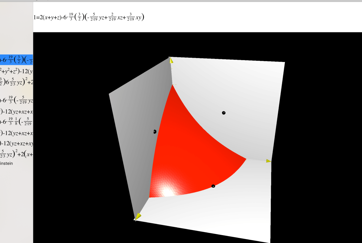
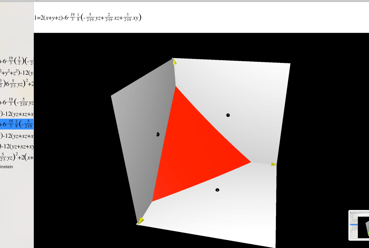
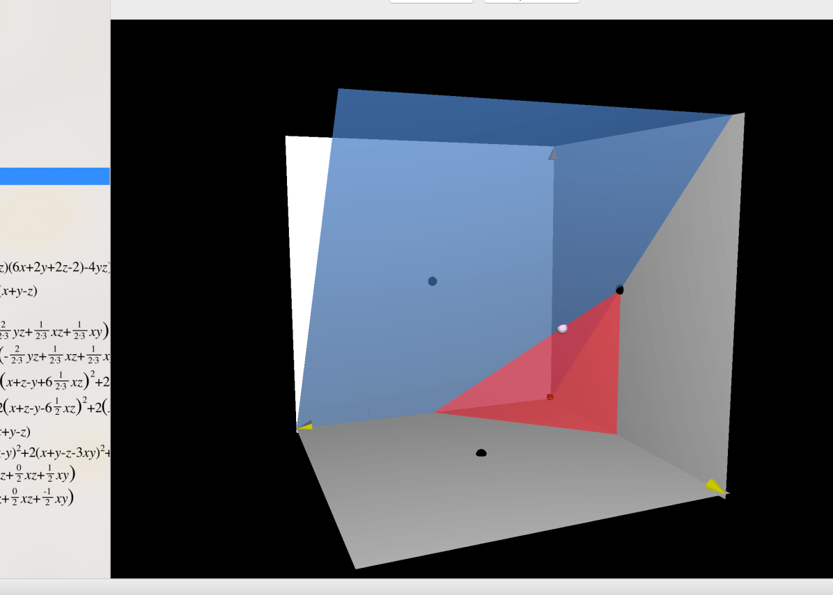
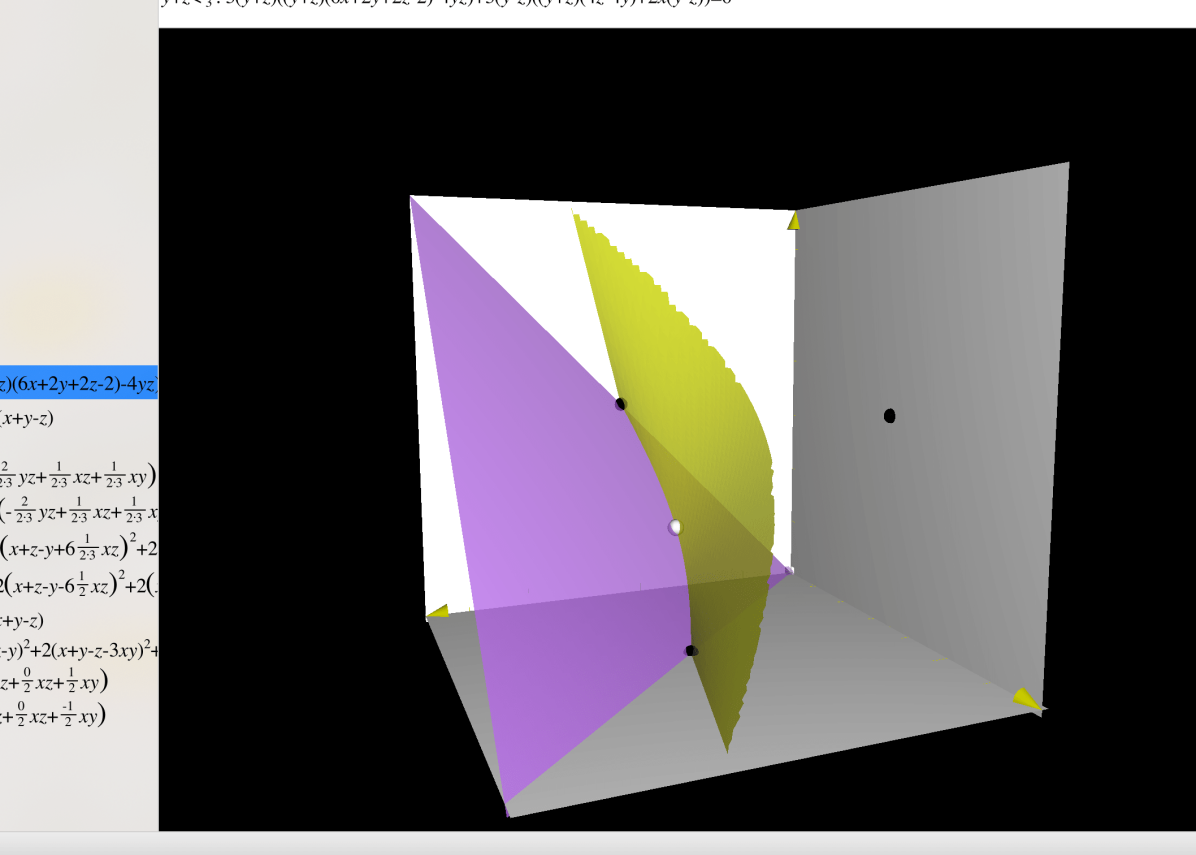
To show that is invariant, it suffices to prove that
| (4.5) |
as demonstrated in Figure 1.
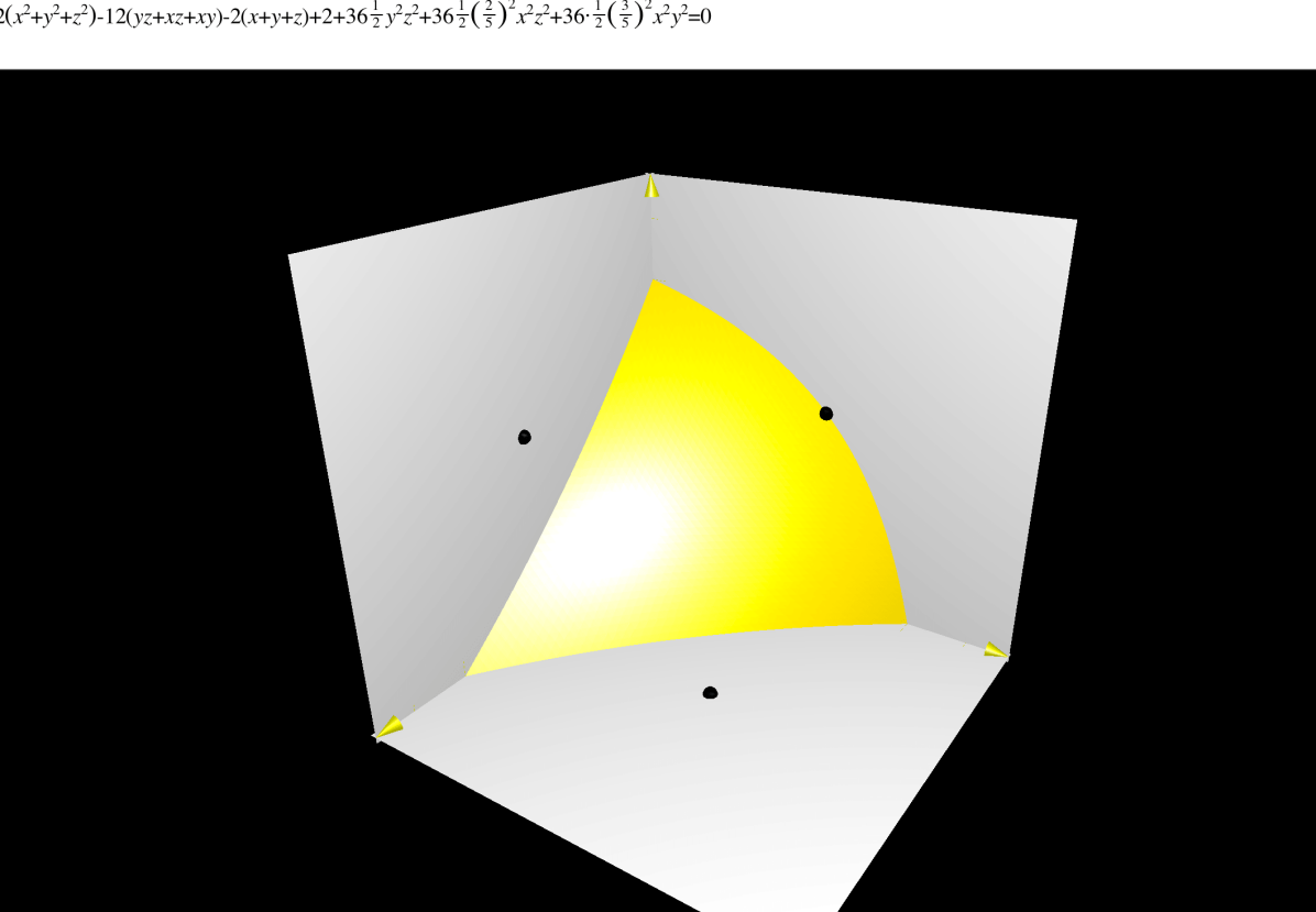
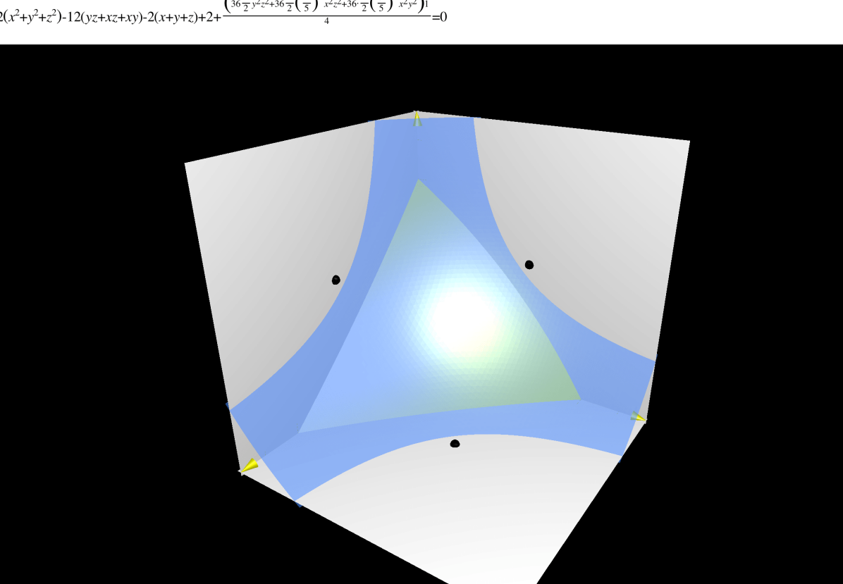
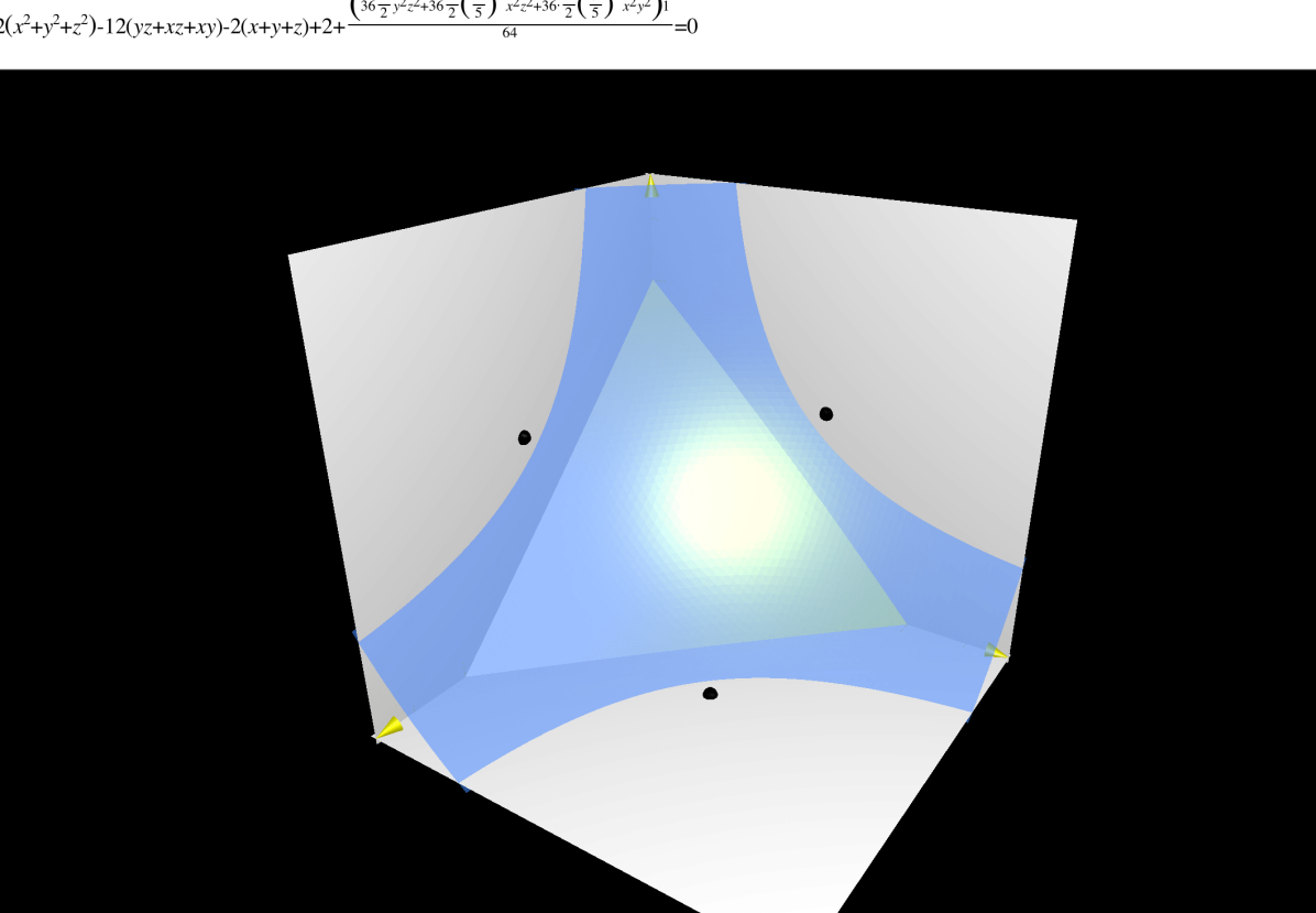
The condition (2.17) plays a key role in proving (4.5). Specifically, we simplify the inequalities by replacing all ’s with ’s. Then the question boils down to showing the separation of two algebraic surfaces in . In order to prove the separation, we find algebraic surfaces that are “ between” the one given by (2.19) and the one from . These so-called “separation surfaces” are symmetric with respect to the hyperplane . In this way, slices of these surfaces with fixed and are easier to be proven to be separated.
Define
| (4.6) |
Proposition 4.2.
Each points in satisfies , i.e.,
Proof.
Define
| (4.8) |
Proposition 4.3.
We have the following inclusion
Proof.
By Proposition 4.2 and Proposition 4.3, to show that , it suffices to prove that
| (4.11) |
The inclusion (4.11) is easier to show since it only involves ’s and polynomials and can be viewed as polynomials in . Specifically, by Proposition 4.1, we know that in . Fix and with , define
| (4.12) |
It is clear that for each fixed , we have
| (4.13) |
It is also clear that has two positive roots for each fixed , with one root be no larger than and the other one no smaller. Let be the smaller positive root of . It is clear that . We have
| (4.14) |
On the other hand, for each fixed , we have
| (4.15) |
Let be the smallest non-negative root of . It is clear that . We then have
Hence (4.11) boils down to proving the following proposition.
Proposition 4.4.
For each fixed ,
Moreover, the equality holds only at .
Proof.
It is clear that . By implicit differentiation, we have
Hence in a small neighborhood around in .
Suppose at some point in . Then and have common roots. Hence the resultant
| (4.16) |
vanishes for some . Straightforward observation in the appendix shows that is non-negative for any and it vanishes only at . Hence and the equality holds only at . The proof is complete. ∎
In summary, we have the following lemma.
Lemma 4.5.
The set is invariant.
Proof.
We have the following chain of inclusions:
| (4.17) |
Therefore we have
| (4.18) |
by Proposition 4.3. In other words, inequality
holds in . Hence we have
| (4.19) |
If non-transverse crossings emerge on an integral curve in , then and at each crossing point. By Proposition 4.2 and Proposition 4.4, we know that and at the crossing point, which force it to be the critical point . Non-transverse crossing is hence excluded and the compact set is invariant. The proof is complete. ∎
4.2 Global Metrics on
One may intend to use the method above to prove the global existence of both and . However, by the following proposition, the method is only effective for the case on .
Proposition 4.6.
The set
| (4.20) |
consists of two connected component, with one of the component being compact.
Proof.
We first prove the statement for . By (2.21), we have
| (4.21) |
Hence either or in . Hence we can write , where is the compact component
Since , the compact component is non-empty. The proof is complete. ∎
Remark 4.7.
Since in , the estimate for can be sharper. From the third last line of computation (4.21), we have
| (4.22) |
Hence in
Remark 4.8.
Now that the construction boils down to showing the inclusion
It turns out that for the case , the analysis is much more delicate than the case . We first state the following proposition.
Proposition 4.9.
The set is invariant.
Proof.
Consider
| (4.24) |
and
| (4.25) |
The proof is complete. ∎
We redefine as
The problem boils down to prove the separation between and . For the case of , the algebraic surface for is too “close” to . It is difficult to find algebraic surfaces such as and in the case of to separate and . Hence in this case, we take algebraic surface given by (2.22) and the one from (2.13) and Proposition 2.4:
Specifically, define
And define
| (4.26) |
With each fixed , and with , we define slices
| (4.27) |
Each pair of slice with fixed gives two polynomials in for us to compare. Since
there is a real positive root for each in . It is clear that for each , has two real roots, with one be no larger than and the other one no smaller. Let be the smaller positive root for each . Since , we let denote the smallest positive root for each . Suppose does not exist, then for that particular slice.
Proposition 4.10.
For each fixed with such that exists, we have
Moreover, the equality holds only at .
Proof.
It is clear that . By implicit differentiation, we have
Hence initially if the direction of derivative as negative component. If the direction of derivative is in the -plane, we consider the function . The Hessian of at is then
The determinant is . Hence in a small neighborhood around in .
Suppose for some , then the resultant of of and vanishes at that point. The formula of is presented in the Appendix. With the help of Maple, we know that is non-negative in the region and it only vanishes at if . If , then vanishes only at and . Therefore for all . ∎
Hence we have the following lemma.
Lemma 4.11.
The set is invariant.
Proof.
We have the following chain of inclusions:
| (4.28) |
Similar to the argument in proving Lemma 4.13, the non-transverse crossing cannot emerge in as the crossing point can only be the critical point . Hence is a compact invariant set. ∎
From Section 3, it is clear that and are in the set and initially if . Hence we have the following lemma.
Lemma 4.12.
Metrics represented by on with are forward complete. Metrics represented by on with are forward complete.
The global existence mentioned in Theorem 1.1 is proven. Our method of proving forward completeness also works on the cohomogeneity one space with exceptional and as principal orbit. For , we obtain two continuous 1-parameter families of metrics with both chiralities on the same manifold . They are part of the more complete family in [Leh20]. For , and are equivalent. In that case, we obtain two continuous 1-parameter families of metrics, one on and the other on . However, such a family does not contain any AC metric and it is a part of the more complete family in Theorem 1.2.
4.3 Global Metrics on and
In this section we prove Theorem 1.2. It turns out that for the case where is the principal orbit, one can have a simpler construction with a larger family of metrics. On , We recover the explicit solution in [CGLP01] and part of the solution in [Baz07]. On , we construct a new continuous 1-parameter family of metric that has geometric transition from the AC Calabi HyperKähler metric to ALC metrics. Such a family was conjectured in [KY02b].
Recall that in [CGLP01], one has an explicit solution to (2.8) with . Specifically, one can impose
for all and obtain a subsystem of (2.8). In the new coordinate, such a subsystem is translated to the invariant subset
Note that this is a 1-dimensional invariant set and critical points and are contained in it. Hence the example in [CGLP01] is transformed to an algebraic curve in the new coordinate. Then we construct the following compact invariant set
Lemma 4.13.
The set is compact and invariant.
Proof.
Since in , we have
| (4.29) |
from (2.19). Since by Proposition 2.1, we know that . Hence computation above continues as
| (4.30) |
Hence , and are bounded above. Therefore is bounded above by (2.19). Then all ’s are bounded. Hence is compact.
It is clear that is invariant. In the subset , we have
| (4.31) |
Hence the proof is complete. ∎
By (3.3), we know that is tangent to if and is in the interior of initially if . Hence is a 1-parameter family of metrics on , and is an AC metric.
Remark 4.14.
Note that for , one can easily show that is invariant. The restricted system of (2.12) on is essentially the same as the one that appears in [Chi21], where a 2-parameter family of non-positive Einstein metrics are constructed, with all Ricci-flat metrics being . Metrics represented by is nothing new but the geometric analogy to metrics in [CGLP02a] and [CGLP02b], belonging to the strictly larger solution set obtained in [Baz08]. The AC metric is the geometric analogy to the metric in [BS89] and [GPP90].
By mimicking the example in [CGLP01], we are able to describe the AC Calabi HyperKähler metric on as an algebraic curve. In fact, integral curve that represents the AC metric sits on the boundary of a compact invariant subset of .
Lemma 4.15.
The set
is compact and invariant. Moreover, the boundary of where both equality hold is an integral curve.
Proof.
Since in , each one of , and is bounded. By (2.22), we know that all ’s are bounded. Then all variables are bounded. The compactness is clear.
We have
| (4.32) |
Since in , computation above continues as
| (4.33) |
On the other hand, we have
| (4.34) |
By multiplying both hand side of last equality in (2.22) by , we know that if ,
| (4.35) |
Hence we have
| (4.36) |
Hence is indeed invariant. ∎
Note that the boundary
is a 1-dimensional invariant set and it contains and . It is clear that is tangent to and is in the interior of initially if . Hence is a 1-parameter family of metrics on , where is an AC metric. In summary, we have
Lemma 4.16.
Metrics represented by on with and are forward complete. Metrics represented by on with and are forward complete. Moreover, metrics and are AC.
By the invariance of and , we also obtain forward complete conically singular metrics with as principal orbits. One can check that for each one of and , there exists a unique unstable eigenvector that is tangent to and , respectively. Integral curves that emanates from and along these eigenvectors lie in . Recall Remark 4.14, we know that they are forward complete. In fact, the integral curve that emanates from is the geometric analogy to in [CGLP02a].
4.4 Asymptotics
Without further specifying, we use to denote either or in Lemma 4.12 and Lemma 4.16 that is defined on is this section. We prove the following.
Proof.
We first consider in Lemma 4.12. By Lemma 4.11, we know that stays in the set where and is held. Since
we know that the function is decreasing along , hence it converges to some limit as . Suppose , then the -limit set of , denoted as , is contained in the level set . By the invariance of the -limit set, we know that . But then by (4.10), we learn that for each point in . Moreover, from (4.10) we know that in implies and . Hence in addition to (2.19), points in also satisfy
From all the constraints above, we can conclude that . By the monotonicity of along and the fact that initially along , we reach a contradiction. Hence
Similarly, we have the monotonicity of along . If does not converges to , then the -limit set is a subset of . Then the -limit can only be , a contradiction.
Hence converges to along each in Lemma 4.12. By Proposition 2.1, it is clear that along . Then from (2.17) and (2.21), we have
| (4.37) |
Since all ’s are bounded above, we must have
Hence is an invariant subset of . The subsystem (2.17) restricted on is essentially the dynamic system of cohomogeneity one metrics with as principal orbit studied in [CS02]. Integral curves that represent smooth cohomogeneity one metric in [BS89] and [GPP90] are included in . In [Chi19b], we show that each integral curve of this subsystem is in fact an algebraic curve in , and . Moreover, they all converges to . By the invariance of , it is clear that . Since is a sink, we conclude that .
Consider in Lemma 4.16, the monotonicity of along imply that functions converges. Suppose the limit is nonzero, then by the invariance of the -limit set and computation similar to (4.31), one can conclude that is satisfied by elements in the -limit set. With (2.19) and the constraints , we know that lies in a straight line . Hence the limit must be .
Theorem 1.1 and Theorem 1.2 are proven by Lemma 4.12, Lemma 4.16 and Lemma 4.17. It is a natural question to ask if metrics on with generic can be extended to a larger family where the boundary is given by an AC metric. If such an AC metric exists, can it be described as an algebraic curve in our new coordinate? A further question is whether one can show is defined on , integral curves that represent cohomogeneity one Ricci-flat metric that may not have any special holonomy.
5 Appendix
5.1 Non-negativity of
We show that for any . Firstly, we have
| (5.1) |
Define function , where
It is clear that and for any . It is also clear that for . Consider
Since
it is clear that any . Since , we have
Hence for any and only vanishes at .
5.2 Formula of
We present the formular for for any . Let , we have
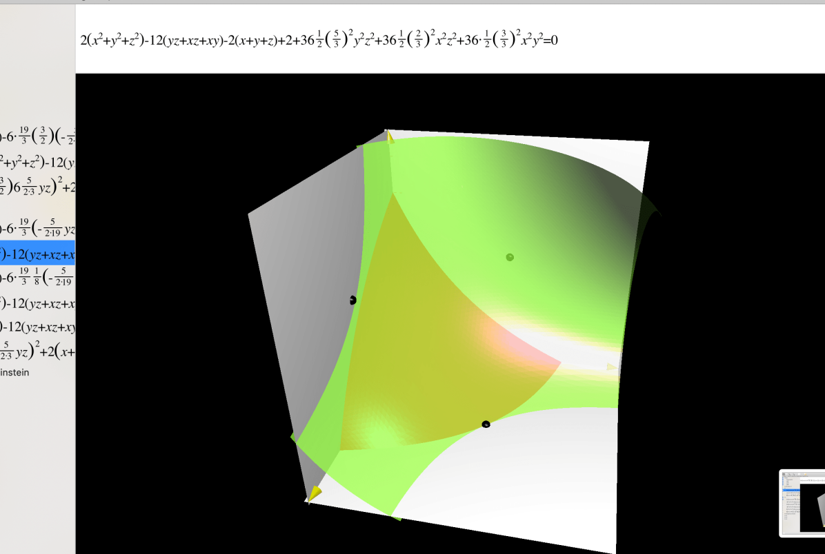
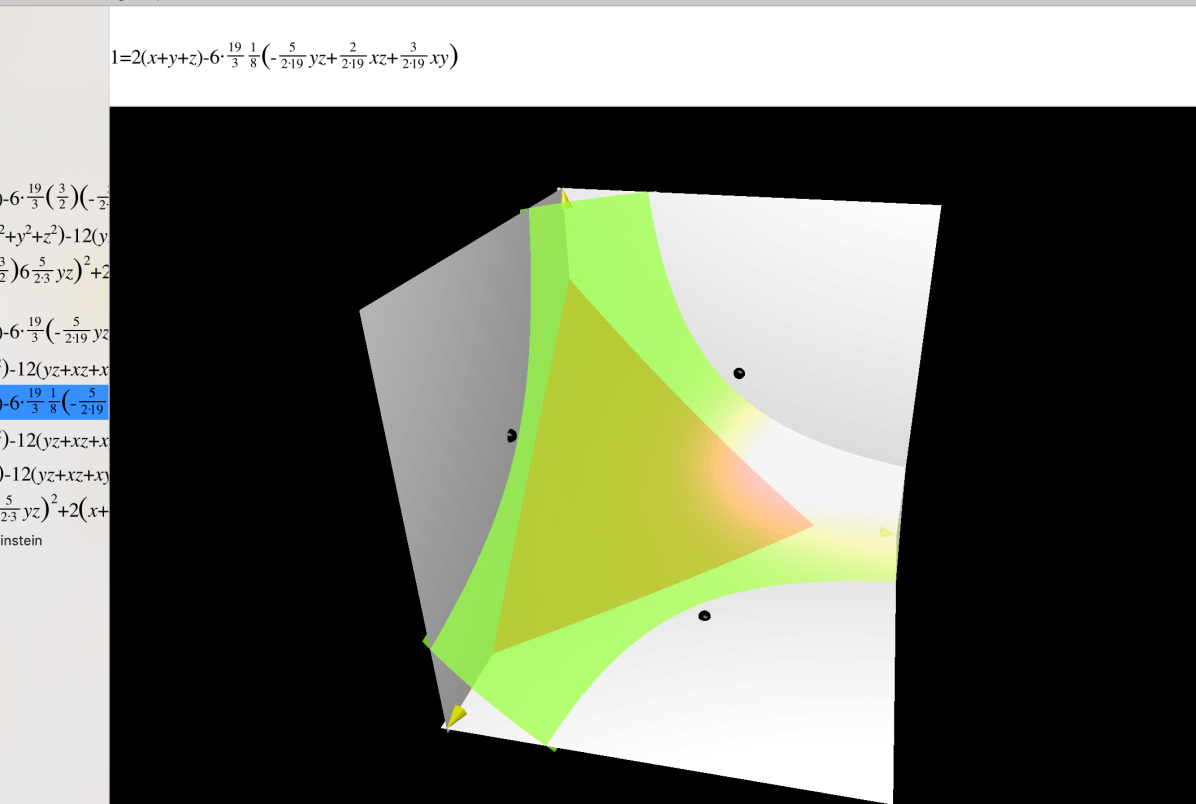
| (5.2) |
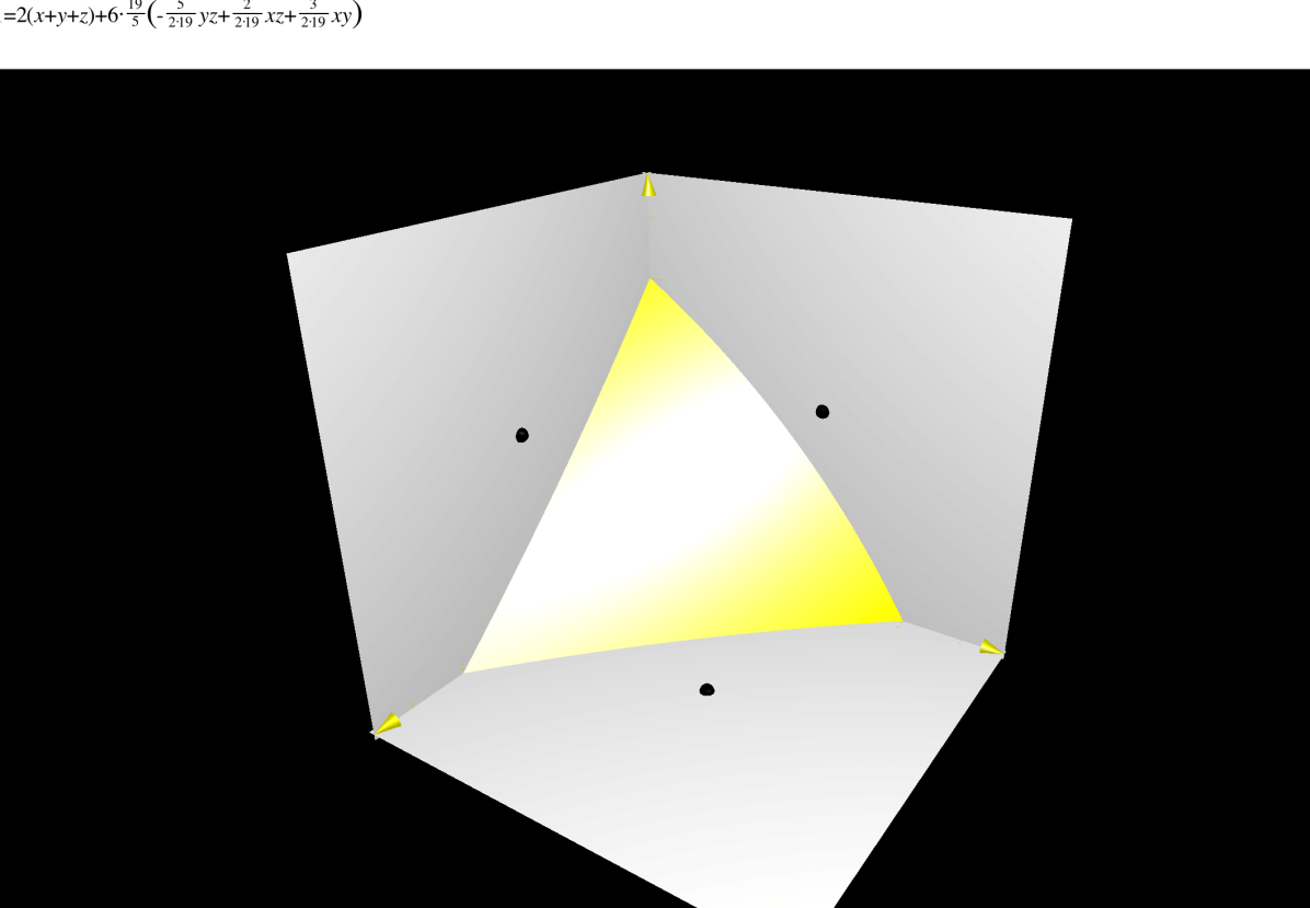
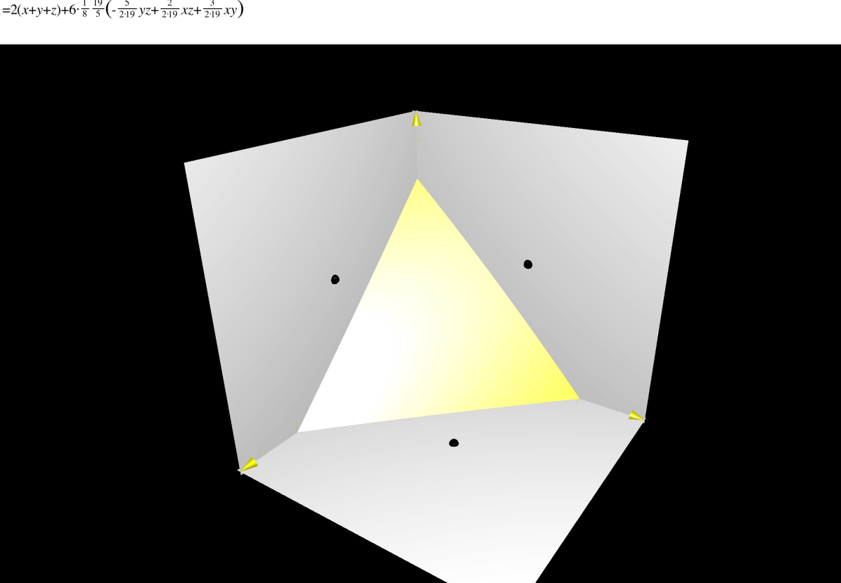
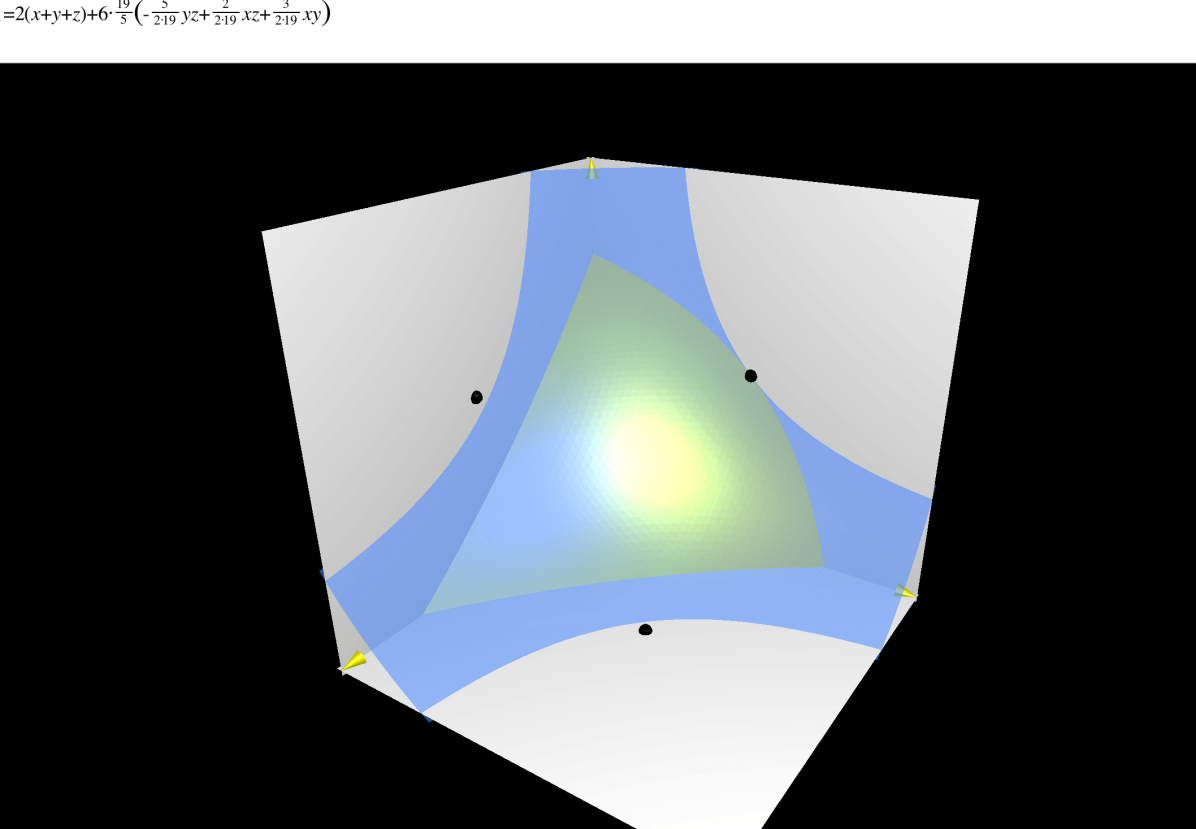
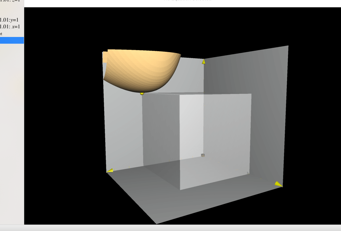
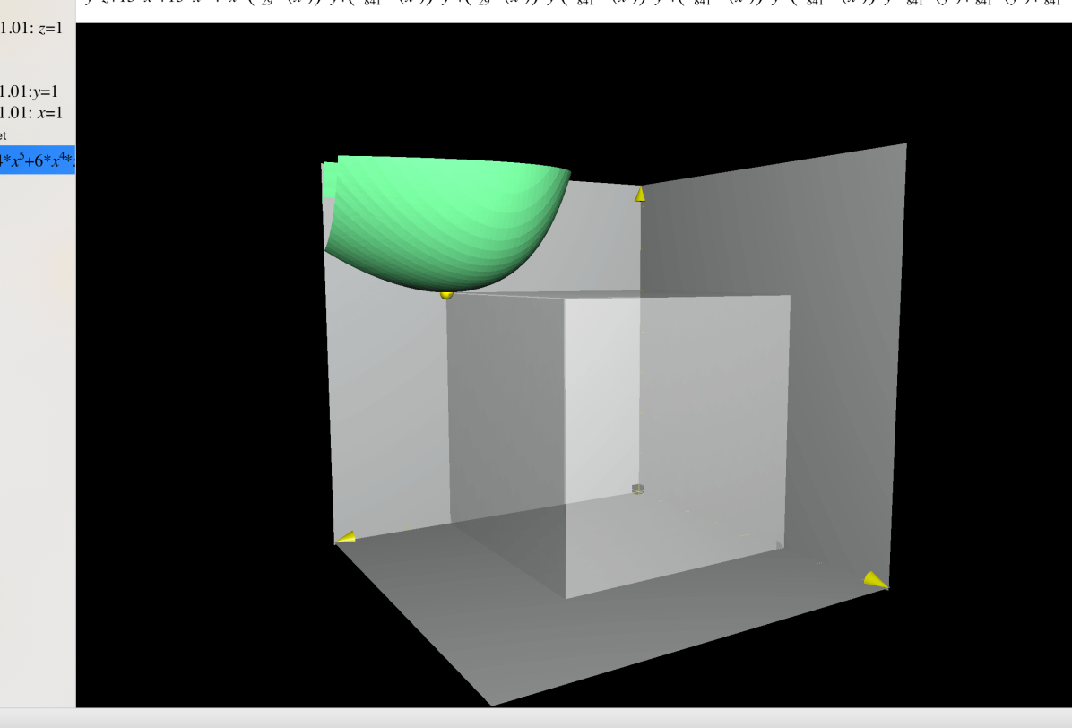
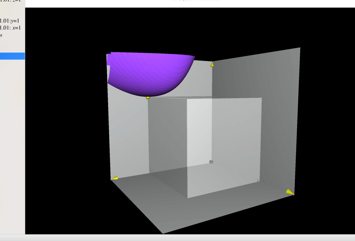
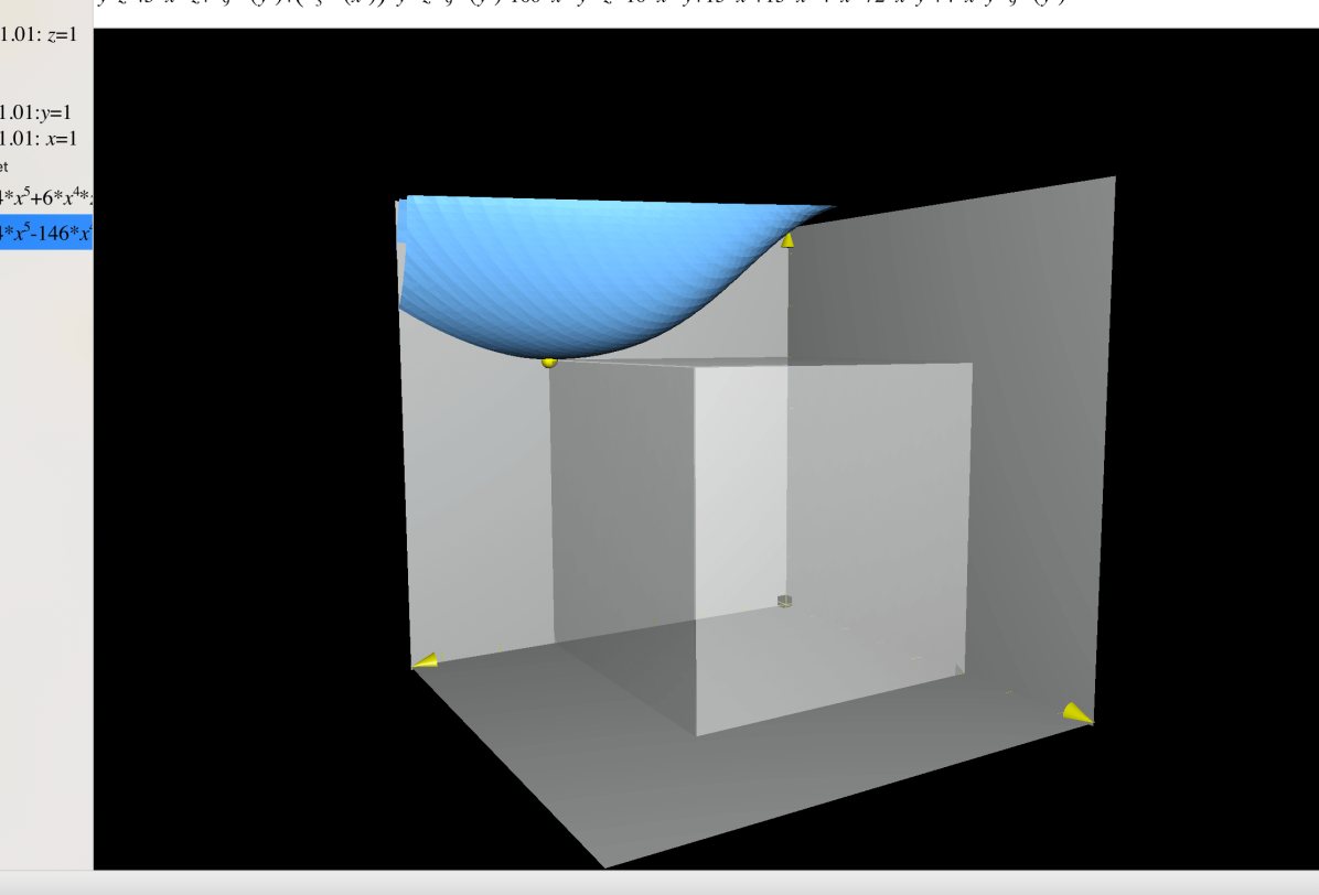
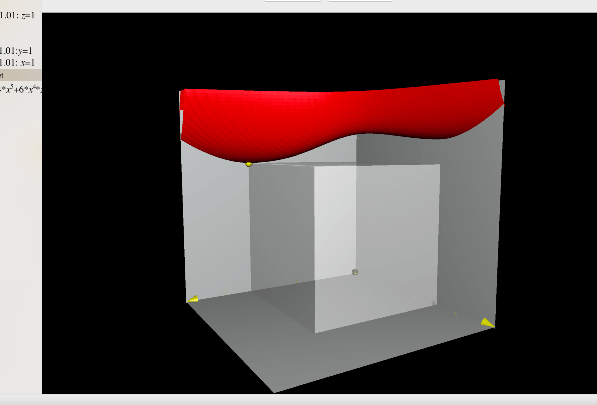
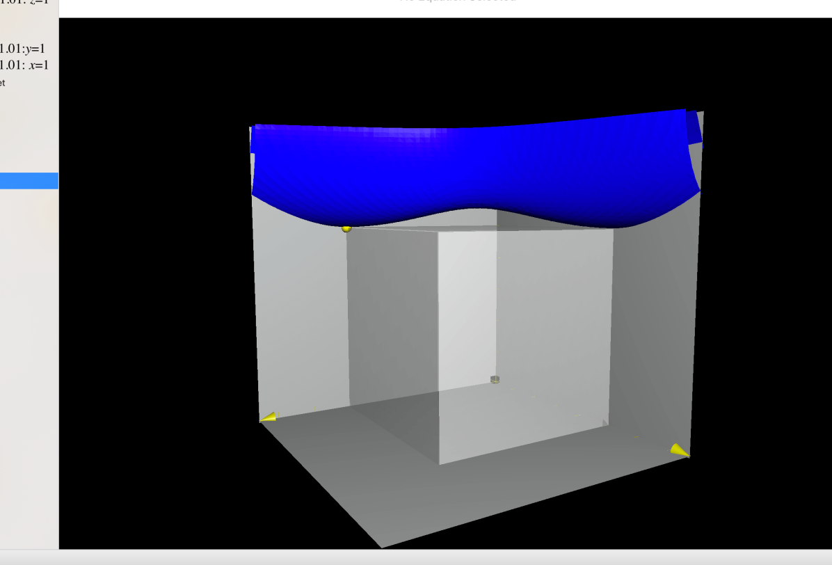
With the help of Maple, one can conclude that for any and it only vanishes at if . If , the function vanishes at and . The level set of with some selected are presented below.
References
- [Baz07] Ya. V. Bazaikin. On the new examples of complete noncompact Spin(7)-holonomy metrics. Siberian Mathematical Journal, 48(1):8–25, January 2007.
- [Baz08] Ya. V. Bazaikin. Noncompact Riemannian spaces with the holonomy group spin(7) and 3-Sasakian manifolds. Proceedings of the Steklov Institute of Mathematics, 263(1):2–12, December 2008.
- [BDW15] M. Buzano, A. S. Dancer, and M. Y. Wang. A family of steady Ricci solitons and Ricci flat metrics. Comm. in Anal. and Geom., 23(3):611–638, 2015.
- [Bon66] E. Bonan. Sur les variétés riemanniennes à groupe d’holonomie ou Spin(7). Comptes Rendus de l’Académie des Sciences, 262:127–129, 1966.
- [Bry87] R. L. Bryant. Metrics with exceptional holonomy. The Annals of Mathematics, 126(3):525–576, November 1987.
- [BS89] R. L. Bryant and S. M. Salamon. On the construction of some complete metrics with exceptional holonomy. Duke Mathematical Journal, 58(3):829–850, 1989.
- [Cal79] E. Calabi. Métriques kählériennes et fibrés holomorphes. Annales scientifiques de l’École normale supérieure, 12(2):269–294, 1979.
- [CGLP01] M. Cvetič, G. W. Gibbons, H. Lü, and C. N. Pope. Hyper-Kähler Calabi metrics, L2 harmonic forms, resolved M2-branes, and AdS4/CFT3 correspondence. Nuclear Physics B, 617(1-3):151–197, December 2001.
- [CGLP02a] M. Cvetič, G. W. Gibbons, H. Lü, and C. N. Pope. Cohomogeneity one manifolds of Spin(7) and holonomy. Physical Review D, 65(10), May 2002.
- [CGLP02b] M. Cvetič, G. W. Gibbons, H. Lu, and C. N. Pope. New complete non-compact Spin(7) manifolds. Nuclear Physics B, 620(1-2):29–54, January 2002.
- [Chi19a] H. Chi. Cohomogeneity one Einstein metrics on vector bundles. PhD Thesis, McMaster University, 2019.
- [Chi19b] H. Chi. Invariant Ricci-flat metrics of cohomogeneity one with Wallach spaces as principal orbits. Annals of Global Analysis and Geometry, June 2019.
- [Chi21] H. Chi. Einstein metrics of cohomogeneity one with as principal orbit. Communications in Mathematical Physics, April 2021.
- [CL55] E. A. Coddington and N. Levinson. Theory of Ordinary Differential Equations. McGraw-Hill Book Company, Inc., New York-Toronto-London, 1955.
- [CS02] R. Cleyton and A. Swann. Cohomogeneity-one -structures. Journal of Geometry and Physics, 44(2-3):202–220, December 2002.
- [DW09] A. S. Dancer and M. Y. Wang. Non-Kähler expanding Ricci solitons. International Mathematics Research Notices. IMRN, (6):1107–1133, 2009.
- [EW00] J.-H. Eschenburg and M. Y. Wang. The initial value problem for cohomogeneity one Einstein metrics. The Journal of Geometric Analysis, 10(1):109–137, 2000.
- [Fos21] L. Foscolo. Complete noncompact Spin(7) manifolds from self-dual Einstein 4–orbifolds. Geometry & Topology, 25(1):339–408, March 2021.
- [GPP90] G. W. Gibbons, D. N. Page, and C. N. Pope. Einstein metrics on and bundles. Communications in Mathematical Physics, 127(3):529–553, 1990.
- [GS02] S. Gukov and J. Sparks. M-Theory on Spin(7) manifolds. Nuclear Physics B, 625(1-2):3–69, March 2002.
- [Joy96] D. Joyce. Compact Riemannian 7-manifolds with holonomy . II. Journal of Differential Geometry, 43(2):329–375, 1996.
- [KV93] O. Kowalski and Z. Vlášek. Homogeneous Einstein metrics on Aloff-Wallach spaces. Differential Geometry and its Applications, 3(2):157–167, June 1993.
- [KY02a] H. Kanno and Y. Yasui. On Spin(7) holonomy metric based on SU(3)/U(1): I. Journal of Geometry and Physics, 43(4):293–309, October 2002.
- [KY02b] H. Kanno and Y. Yasui. On Spin(7) holonomy metric based on SU(3)/U(1): II. Journal of Geometry and Physics, 43(4):310–326, October 2002.
- [Leh20] F. Lehmann. Geometric transitions with Spin(7) holonomy via a dynamical system. arXiv:2012.11758 [math], December 2020.
- [Rei08] F. Reidegeld. Spin(7)-manifolds of cohomogeneity one. PhD Thesis, Technische Universität Dortmund, 2008.
- [Rei11] F. Reidegeld. Exceptional holonomy and Einstein metrics constructed from Aloff–Wallach spaces. Proceedings of the London Mathematical Society, 102(6):1127–1160, June 2011.
- [VZ20] L. Verdiani and W. Ziller. Smoothness conditions in cohomogeneity one manifolds. Transformation Groups, September 2020.
- [Win17] M. Wink. Cohomogeneity one Ricci Solitons from Hopf Fibrations. arXiv:1706.09712 [math], June 2017.