Spitzer Microlensing of MOA-2016-BLG-231L : A Counter-Rotating Brown Dwarf Binary in the Galactic Disk
Abstract
We analyze the binary microlensing event MOA-2016-BLG-231, which was observed from the ground and from Spitzer. The lens is composed of very low-mass brown dwarfs (BDs) with and , and it is located in the Galactic disk . This is the fifth binary brown dwarf discovered by microlensing, and the BD binary is moving counter to the orbital motion of disk stars. Constraints on the lens physical properties come from late time, non-caustic-crossing features of the Spitzer light curve. Thus, MOA-2016-BLG-231 shows how Spitzer plays a crucial role in resolving the nature of BDs in binary BD events with short timescale ( days).
Subject headings:
binaries: general - brown dwarfs - gravitational lensing: micro1. introduction
Brown dwarfs (BDs) are substellar objects that are not massive enough to burn hydrogen. BDs have a mass between gas giant planets and low-mass stars, and it is thought that the formation and evolution of BDs are different from those of planets and stars (Ranc et al., 2015). Thus, studying BDs is helpful to understand the formation and evolution of stars and planets.
Microlensing is an excellent method to detect faint low-mass objects, such as BDs and planets because it does not depend on the light from the objects, but the mass. Until now 32 BDs have been detected by microlensing. Only five of these are isolated BDs, while all the others belong to binary systems. Microlensing BDs are mostly binary companions to faint M dwarf stars (see Table 1), while most of the many BDs detected by the radial velocity, transit, and direct imaging methods are companions to solar-type stars (Ranc et al., 2015). Hence, microlensing BDs are important to constrain BD formation scenarios including turbulent fragmentation of molecular clouds (Boyd & Whitworth, 2005), fragmentation of unstable accretion disks (Stamatellos et al., 2007), ejection of protostars from prestellar cores (Reipurth & Clarke, 2001), and photo-erosion of prestellar cores by nearby very bright stars (Whitworth & Zinnecker, 2004).
However, with microlensing, it is generally difficult to measure the mass of a lens. This is because we usually obtain only the Einstein timescale,
| (1) |
where is the angular Einstein radius corresponding to the total lens mass and is the relative lens-source proper motion. For the measurement of the lens mass, one needs to measure the angular Einstein radius and microlens parallax , which yields
| (2) |
where is the lens-source relative parallax, and are the distances to the lens and source, respectively, and (Gould, 2000). The angular Einstein radius can be measured from events with finite-source effects, while the microlens parallax can be measured from the detection of light-curve distortions induced by the orbital motion of Earth on a standard microlensing light curve (Gould, 1992, 2013). The large number of microlensing BDs detected to date would appear to indicate that M dwarf-BD binaries and BD binaries are very common. This is because their mass measurements (hence, unambiguous determination that they are BDs) require clear detection of a microlens parallax signal that can be detected from the ground despite a relatively short timescale. However, it is usually very difficult to measure the microlens parallax, especially for short timescale events, such as M dwarf-BD binaries. While the microlensing parallax (derived from Equation(2))(Gould, 2000)
| (3) |
is on average large for low-mass lenses, this is not by itself usually sufficient to render it measurable in short events. Rather, large is required as well. As a result, half (7/13) of microlensing binaries containing at least one BD and with mass measurements based on ground-based microlensing parallaxes have distances kpc, which would be true of a tiny fraction of all microlensing events. Moreover, of the remainder, all lie in the Galactic disk kpc, and almost all have low, or very low proper motions (so long, or very long timescales), which again is rare.
Hence, it is important to check independently that these relatively frequent detections are not just due to systematics misinterpreted as parallax signal”. The Spitzer satellite allows us to do that. Spitzer observations together with ground-based observations yield the microlensing parallax, which does not depend strongly on the event timescale and lens distance. Thus, Spitzer makes it possible to measure the masses of the lenses in short binary BD events, which would be quite difficult using only ground-based observations. The microlens parallax is measured from the difference in the light curves as seen from the two observatories with wide projected separation (Refsdal S., 1966; Gould, 1994), which is represented by
| (4) |
where
| (5) |
and where the subscripts indicate the parameters as measured from the satellite and Earth. Here is the time of the closest source approach to the lens (peak time of the event) and is the separation between the lens and the source at time .
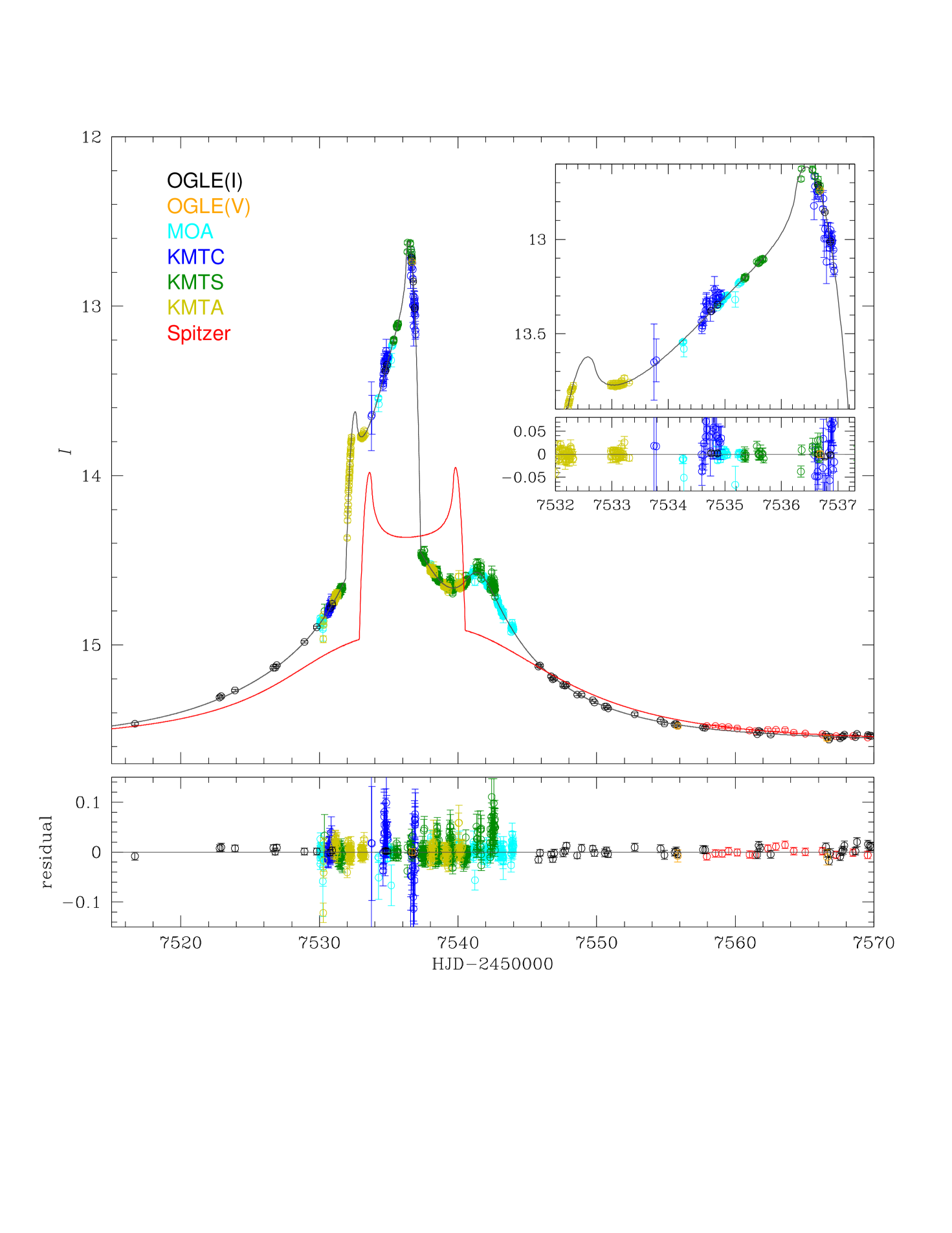
In this paper, we report the discovery of the fifth binary BD from the analysis of the microlensing event MOA-2016-BLG-231, which was observed from the ground and from Spitzer. Although Spitzer can identify binary BDs events with short , observing such events is extremely challenging because of the short timescale and the day observation delay (see Figure 1 of Udalski et al. 2015). Thus, Spitzer does not usually observe caustic crossings of such events. However, we here show that even non caustic-crossing Spitzer light curves can resolve the nature of a binary BD lens.
2. OBSERVATIONS
2.1. Ground-based observations
The microlensing event MOA-2016-BLG-231 was first alerted on UT 22:18 6 May by the Microlensing Observations in Astrophysics (MOA; Suzuki et al. 2016). MOA uses a 1.8 m telescope with 2.2 deg2 field-of-view (FOV) at Mt. John Observatory in New Zealand. The lensed source star is at = , corresponding to . The Early Warning System (EWS) of the Optical Gravitational Lensing Experiment (OGLE) collaboration (Udalski A., 2003) also alerted this event 7 days after the MOA alert. OGLE uses the 1.3 m Warsaw telescope at the Las Campanas Observatory in Chile. The event is located in the OGLE field BLG501, which is observed with cadence . The event is designated as OGLE-2016-BLG-0864 by OGLE. Here we note that although MOA first alerted the event, Spitzer observations were triggered by OGLE data rather than MOA, and MOA did not play a major role in characterization of the lens. Since the Einstein crossing time of the event is short , and the OGLE baseline is slightly variable on long timescales, we used only 2016 season data sets of OGLE and MOA for light curve modeling.
The event was also observed by the Korea Microlensing Telescope Network (KMTNet; Kim et al. 2016). KMTNet uses 1.6 m telescopes with 4.0 deg2 FOV at CTIO in Chile (KMTC), SAAO in South Africa (KMTS), and SSO in Australia (KMTA). MOA-2016-BLG-231 lies in two overlapping KMTNet fields, BLG01 and BLG42, with a combined cadence of . It is designed by KMTNet as KMT-2016-BLG-0285 (Kim et al., 2018). Most of KMTNet data were taken in band, and for the characterization of the source star, some data were taken in band from CTIO. The KMTNet data were reduced by pySIS based on the difference imaging method (Alard & Lupton, 1998; Albrow et al., 2009).
2.2. Spitzer observations
Since 2014, Spitzer has been observing microlensing events toward the Galactic bulge in order to measure the microlens parallax. While the overwhelming majority of events chosen for Spitzer observations are (apparently) generated by point-mass lenses at the time of selection, in accordance with the detailed protocols described by Yee et al. (2015), the Spitzer team does select known binary and planetary lenses whenever there appears to be a reasonable chance to measure the microlens parallax. MOA-2016-BLG-231 was such a case. At the time of selection, the event was regarded by the team as “difficult, but maybe doable” because it was recognized that the timescale of event was quite short and the first Spitzer observation would be 15 days after the final anomalous feature in the light curve. See Figure 1. It was observed for three weeks, mostly at a cadence of , but roughly double that for the first few days because of the limited number of available events due to Spitzer’s sun-angle exclusion of more easterly targets.
3. LIGHT CURVE ANALYSIS
3.1. Ground-based data
The observed ground-based data of the event MOA-2016-BLG-231 have a clear caustic-crossing feature, while the Spitzer data (as anticipated) show only a general decline. We therefore begin by incorporating only ground-based data to conduct binary lens modeling. Standard binary lens modeling requires seven parameters including three single-lens parameters (, , ) and four additional parameters: the projected separation of the lens components in units of (), the mass ratio of the components (), the angle between the source trajectory and the binary axis (), and the normalized source radius () (Rhie et al., 1999), where is the angular radius of the source. In addition, there are two flux parameters for each observatory, the source flux and blended flux of the ith observatory. The two flux parameters at a given time are modeled by
| (6) |
where is the magnification as a function of time at the ith observatory (Rhie et al., 1999). The two flux parameters of each observatory are determined from a linear fit.
We conduct a grid search in the parameter space to find the best-fit model. The ranges of the parameters are , , and , respectively. During the grid search, the other parameters are searched for using by a Markov Chain Monte Carlo (MCMC) method. The magnification is calculated by inverse ray shooting near and in the caustic (Kayser et al., 1986; Schneider & Weiss, 1988; Wambsganss, 1997) and multipole approximations (Pejcha & Heyrovský, 2009; Gould, 2008) otherwise. From this, we find only one local minimum at . We then seed the local solutions into the MCMC for which all parameters are allowed to vary, and finally find a global solution of the binary lens model.
As in many binary and planetary events, can be measured from the effect of the finite size of the source to smooth the intrinsically divergent magnification profile of the caustic. Because the source crosses the caustic, we consider the limb-darkening variation of the finite source star in the modeling. For this, we adopt the source brightness profile, which is approximated by
| (7) |
where is the total flux of the source at wavelength , is the limb darkening coefficient, and is the angle between the normal to the surface of the source star and the line of sight (An et al., 2002). According to the source type, which is discussed in Section 4, we adopt that , , and from Claret (2000) and Claret & Bloemen (2011).
3.2. Combination of ground-based and Spitzer data
Thanks to the Spitzer data, we can constrain the higher-order effects of microlensing parallax and lens orbital motion, even though days would not be long enough to detect these two effects using ground-based data alone. When including the parallax effect in the model, it is important to include also the orbital motion effect because of the degeneracy between the two (Skowron et al., 2011; Batista et al., 2011; Han et al., 2016). Thus, we conduct the modeling with both parallax and orbital effects. The microlens parallax enters as a two-parameter vector , whose amplitude is given by Equation (4) and whose direction is that of the lens-source relative proper motion in the geocentric frame, i.e., . Under the approximation of linear orbital motion of the binary lens, the orbital motion effect is described by two parameters, and , which are the change rates of the binary separation and the orientation angle of the binary axis, respectively. Hence, four additional parameters are added in the model. In contrast to the ground-based light curve, Spitzer covers only the falling wing of the light curve. Thus, it is essential to incorporate the color constraint between OGLE and Spitzer in order to find the correct parallax solution. See, for example, the analysis of OGLE-2016-BLG-0168 by Shin et al. (2017). We find by combining the source instrumental color measurement, which is discussed in Section 4, with a instrumental color-color relation derived from matched field stars. To enforce the color constraint, we add a to calculated in the model, which is defined as
| (8) |
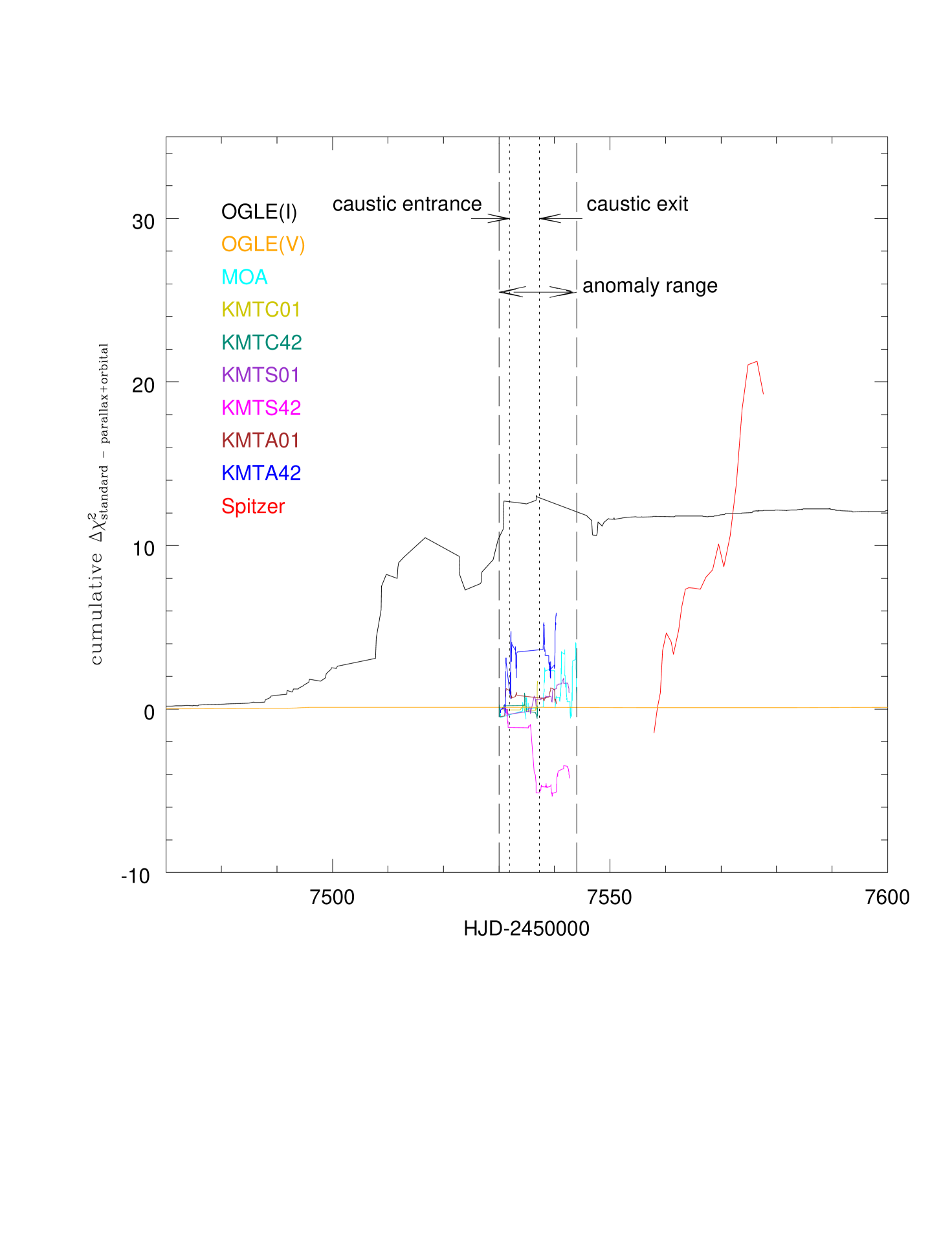
where and are the source fluxes of OGLE and Spitzer, which are obtained from the model, and is the error of the color constraint . Thus, = . In order to find correct source and blended fluxes of Spitzer, and , with a strong color constraint, we include them as chain variables when modeling. Because of the low value of , we expect most of the microlens parallax “signal” to come from Spitzer and not the ground-based data. However, we find that when we model the event using all data sets, most of these contribute signal at the of few tens level (and with different signs), with these signals coming overwhelmingly from the wings of the event, as determined from a cumulative plot (see further below). Such false parallax signals are not uncommon in MOA data, and have also been seen in KMTNet data during its much shorter history. Therefore, we restrict all ground-based data sets except OGLE to the time interval , where the rapid changes in magnification ensure that very low-level systematics will not play any significant role. We then find that the cumulative distribution of shows no strong trends in any of the data sets except Spitzer. See Figure 2.
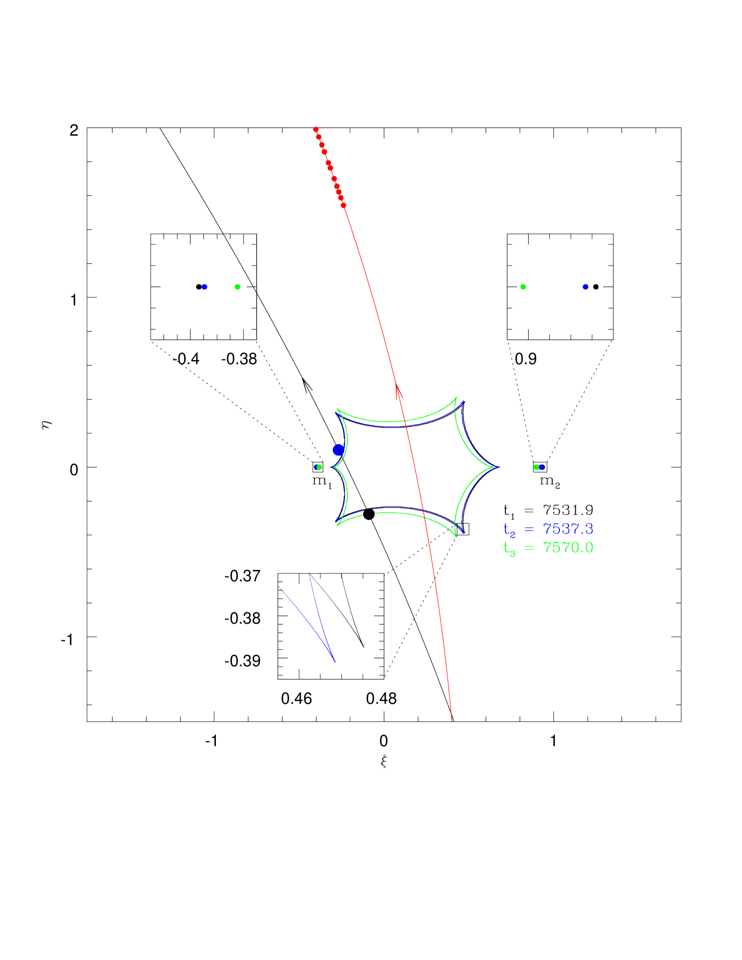
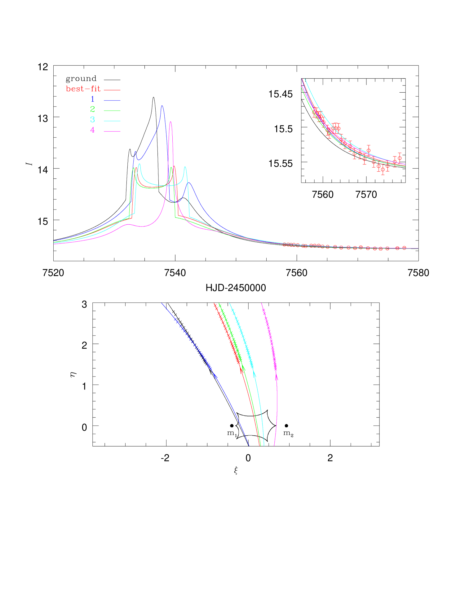
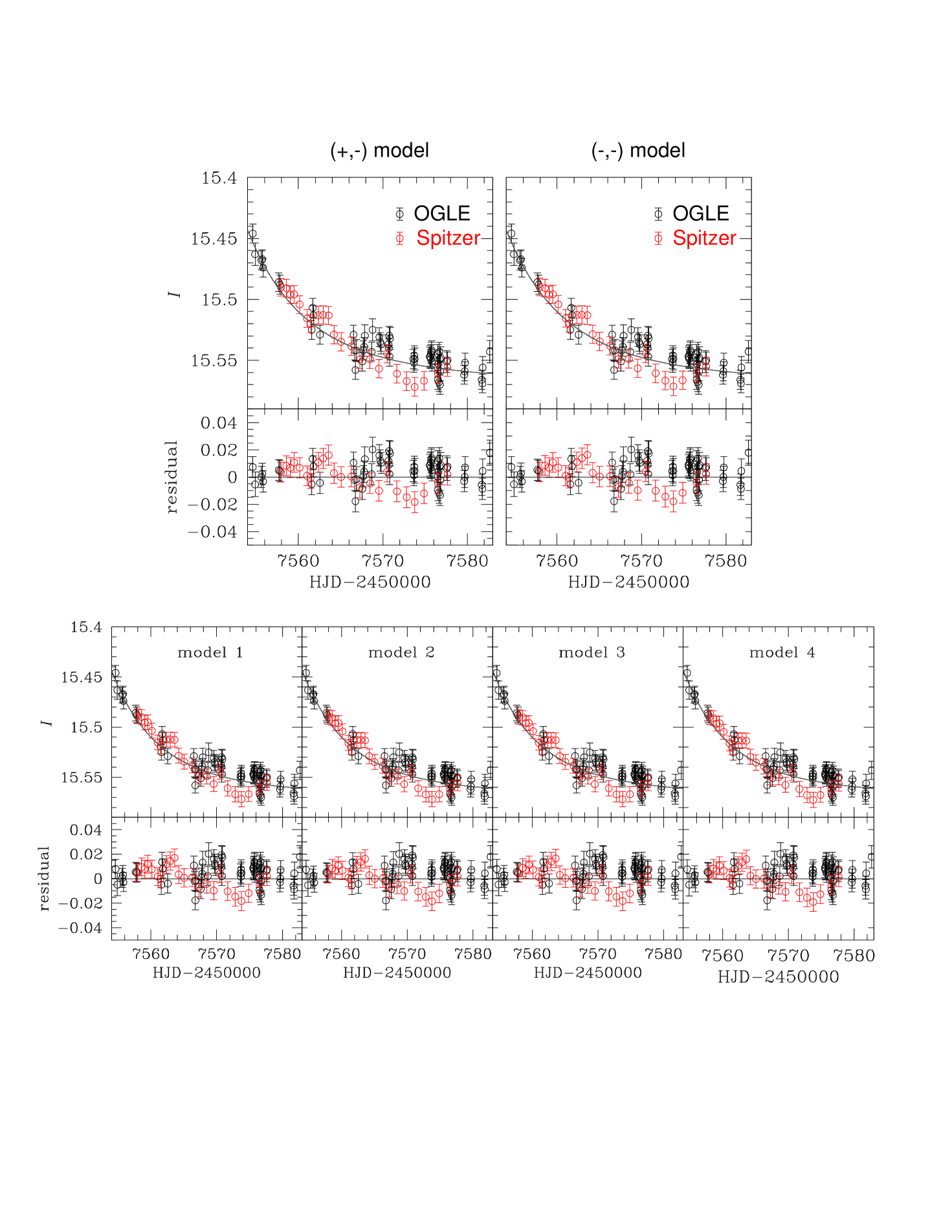
Observations from the ground and from Spitzer yield a well-known four degeneracy for the microlens parallax : , , , and , which register the signs of the impact parameters as measured from the ground and Spitzer, respectively (Zhu et al., 2015). From the modeling, we find that the event MOA-2016-BLG-231 has only two solutions, and , and that the solution is preferred by . The other models and converge to and models, respectively. The best-fit lensing parameters of the and models are presented in Table 2. Figure 1 shows the best-fit light curve of the event, i.e., for the model. The corresponding source trajectories for the ground and Spitzer are presented in Figure 3. Figure 3 also shows the caustic structures and positions of the lens components at three different epochs, (caustic entrance), (caustic exit), and (close to baseline). As shown in Figure 3, the caustics and lens positions at the two epochs ( and ) appear almost the same. This is because the characteristic orbital timescale, is long compared to the time interval explored . Here, . While the improvement of the parallax+orbital solution compared to the parallax-only solution is relatively small, , we will argue in Section 5 that this detection of orbital motion is likely real.
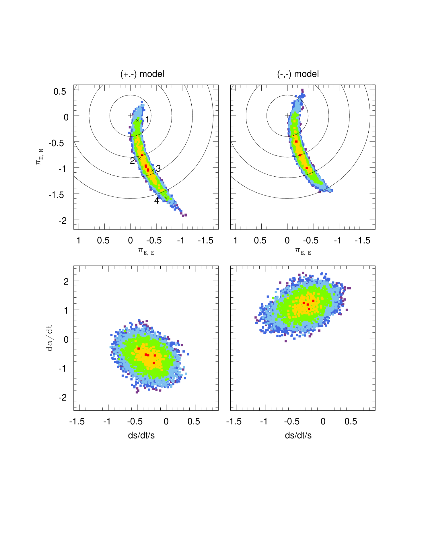
Figure 4 shows distributions of the parallax and orbital motion parameters for the and models. The parallax amplitude is quite well constrained and very similar in the two cases, implying that the mass and distance of the system will be both well measured and not seriously impacted by the two-fold parallax degeneracy. From this, we find that even though Spitzer has no caustic-crossing features and it has only fragmentary coverage of the light curve, we can constrain the physical properties of lens.
In Figure 4, we mark four representative models for , which are located just inside the contour. The corresponding parallax and orbital parameters are presented in Table 2. Figure 5 shows the Spitzer trajectories and resulting light curves of the four models. As shown in Figure 5, these four models have different trajectories from the best-fit one, and hence dramatically different predicted Spitzer light curves over the peak of the event. However, during the time interval that Spitzer actually took data, all four predict similar light curves (see the inset to Figure 5). Despite these different trajectories, and as discussed above, these have qualitatively similar amplitudes, , which is what enables a mass measurement.
4. Estimate of
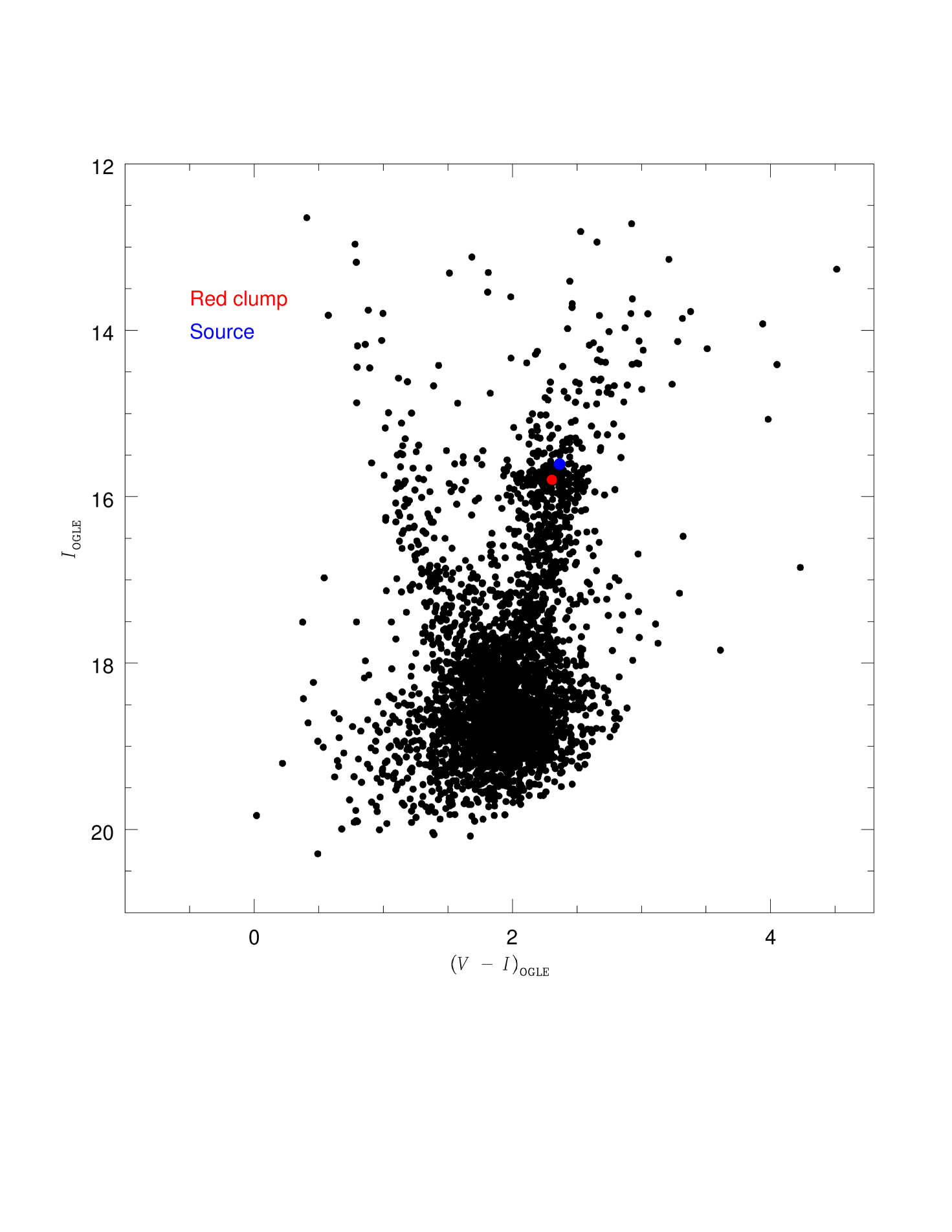
As mentioned in Section 1, and should be measured for the measurements of the mass and distance of the lens. Thanks to caustic-crossing features, one measure from the modeling, while . Thus, we need to estimate for the measurement of . We estimate from the intrinsic color and brightness of the source, which can be derived by the offset between the source and the red clump in the instrumental color and magnitude diagram (CMD) (see Fig. 6) (Yoo et al., 2004). These are determined by
| (9) |
where is the offsets of the color and brightness between the source and the clump. We determine the instrumental source color by regression of the on flux measurements and derive the source instrumental magnitude from the model. These have errors of 0.004 and mag, respectively. We then centroid the clump in color and magnitude with errors of 0.022 and 0.05 mag respectively. The measured color and magnitude offsets are . Adopting from Bensby et al. (2011) and Nataf et al. (2013), we find . This indicates that the source is a K-type giant. We determine the angular radius of the source using color-color relation (Bessell & Brett, 1988) and the color/surface brightness relation (Kervella et al., 2004). As a result, we find that . With the measured and , we determine the angular radius of the Einstein ring corresponding to the total mass of the lens,
| (10) |
The relative lens-source proper motion is
| (11) |
5. Lens properties
Using the estimated and , we measure the total mass of the lens system,
The lens is composed of low-mass BDs with masses and , where , and the projected separation of the two BDs is au. The relative parallax between the lens and the source is
| (12) |
Assuming that the source is located at 8.3 kpc (Nataf et al., 2013), we estimate the distance to the lens,
| (13) |
Hence, the lens is a BD binary located in the Galactic disk. This is the fourth BD binary discovered by microlensing. Because is well measured due to a precise measurement, which comes from good coverage of caustic-crossing, the errors in the mass and distance of the lens primarily reflect the error in . As shown in Figure 4, the correlation between and components is not well approximated by a linear relation. Hence, we use the best-fit MCMC chains to determine the errors in physical lens parameters including the mass and distance of the lens. Then, one can determine the standard deviation of each physical parameter from the chains. Thus, physical lens parameters in Table 3 represent the median values of each physical parameter from the and MCMC chains, and their error bars represent the 16th and 84th percentile values of each parameter from the chains.
In order to check that the binary lens is a bound system, we compute , i.e., the ratio of the projected kinetic to potential energy (An et al., 2002),
| (14) |
where . Since (or for model) represents very typical values for a bound pair seen at random orientation, and in particular indicates that the lens system satisfies the condition of a bound system, (An et al., 2002), it is valid. We list estimated physical parameters of the lens system in Table 3. In Table 3, we also list physical lens parameters for four models with from Figures 4 5. Three of the four models imply that the lens system is a low-mass BD binary in the disk, similar to the best-fit solutions, while for model 1 it is a binary composed of a low-mass star and a BD in the disk. This is because of large uncertainties of , as shown in Figure 4. We further discuss these models of the lens system in Section 6.
6. DISCUSSION
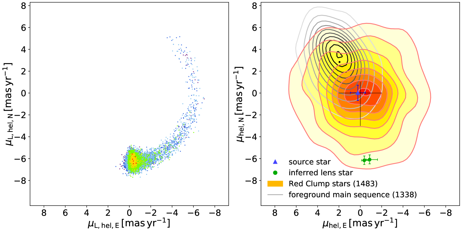
Table 2 shows that all for two best models is negative. This means that the lens located in the Galactic disk is moving in the opposite direction to the disk orbital motion. It is unusual. In order to check that it is real, we conduct the modeling under the condition that high-order effect parameters set to zero and the initial values of the other standard model parameters including Spitzer fluxes set to the best-fit solutions of the two parallax+orbital models including and . We also conduct the same test for the four models indicated in Figure 4. As a result, we find that for all of the six models the slope of the Spitzer fluxes is steeper than the model (see Figure 7). This means that Spitzer observed the event later than Earth, and the lens is moving toward Spitzer, i.e., toward the west. Therefore, it is real that the lens is moving in the opposite direction to the disk orbital motion. In addition, in order to demonstrate that the lens is moving west relative to the source, we measure the proper motion of the source (see Figure 8). We find that . As shown in Figure 8, the source is certainly part of the bulge population and is not moving relative to the bulge stars. Hence, the measurement of the lens-source relative motion clearly means that the lens is not moving with the disk. With the measurement of the source proper motion, we can measure the heliocentric proper motion of the lens,
| (15) |
where is the velocity of Earth at the peak of the event and projected perpendicular to the directory of the event. For this case, . From Equation (14), we find that for solution, while for solution, . From the measurement of , we can also measure the transverse velocity of the lens, (Shvartzvald et al., 2018),
| (16) |
where . Here are the transverse components of the Sun’s peculiar velocity relative to the Local Standard of Rest and is the disk circular velocity. Thus, the peculiar velocity of the lens relative to the mean motion of the Galactic disk stars (Shvartzvald et al., 2018) is
where because both lens and Sun are disk stars. From Equation (16), we find that for two degenerate solutions, and , and , respectively. This means that the lens is counter-rotating relative to the motion of Galactic disk stars. In order to check that the four models with in Figure 4 are compatible with the two solutions, we also estimate the proper motions and peculiar velocities of the lens for the four models, and they are as follows as
The lens proper motions of the four models are consistent with those of the two best-fit solutions. Therefore, the lens is a counter-rotating disk object. Until now two counter-rotating disk objects (OGLE-2016-BLG-1195L (Shvartzvald et al., 2017), OGLE-2017-BLG-0896L (Shvartzvald et al., 2018)) have been discovered by microlensing, the first being right at the hydrogen-burning limit and the second being a low-mass BD. MOA-2016-BLG-231L is the third such object, and it is the first counter-rotating BD binary discovered by Spitzer. The unusual kinematics of the BD binary suggest that the BD binary could be a halo object or a member of counter-rotating low-mass object population, as mentioned in Shvartzvald et al. (2018).
For the event MOA-2016-BLG-231, it is found that there is an extremely small offset between the source position and the baseline object. The offset is 0.05 pixels, and it corresponds to mas. This means that the blend could be associated with the event. However, the blended flux is in fact consistent with zero. First, the formal estimate of the blended flux is , where one unit of flux corresponds to . This in itself is consistent with zero at the level. Moreover, the estimate of is ultimately derived from , where is the source flux from the microlensing model and comes from DoPhot (Schechter al., 1993) photometry of this field location. Because of the mottled background of unresolved turnoff stars in these croweded fields, can easily have errors at this level. Therefore, there is no clear evidence for blended light. In addition, we measure using OGLE deep stack images. From this, we find that from the deep stack images is 0.06 mag brighter than the value obtained from the OGLE reference images (i.e. normal OGLE data) due to a nearby star at . Hence, cannot be estimated from the reference image photometry to better than 0.06 mag due to the presence of the nearby star. Therefore blended light cannot be determined better than 0.5 flux units. This reinforces the naive conclusion that there is no evidence for light from the lens.
The result of modeling with chain variables and yields negative (see Table 2). (see Table 2). This is somewhat unusual. As reported in Calchi Novati et al. (2015) and Shvartzvald et al. (2018), the negative Spitzer blending can be generated when the flux of unresolved faint stars is included in the global background flux. The event OGLE-2017-BLG-0896 (Shvartzvald et al., 2018) is also the event affected by the excess flux due to unresolved stars and has almost the same Spitzer blending as this event.
The result of this study indicates that the lens system of MOA-2016-BLG-231 consists of two low-mass BDs. In principle, there are two scenarios that would drive us to very different conclusions, but neither of them is likely to be true. First, a smaller parallax value would give a more massive and more distant lens system. For example, out of the four models indicated in Figure 4, model 1 has the smallest parallax, which produces the most massive and the most distant lens system and thus might in principle solve the puzzle on the counter-rotating motion. However, the model 1 gives a low-mass M dwarf-BD binary with at a distance of , which still implies that it is in the disk. Moreover, with proper motion , it is still counter-rotating. Therefore, the smaller parallax scenario is unlikely to resolve the issue of a counter-rotating lens. Furthermore, for the other models, all the lens systems are low-mass BD binaries with that is located at the disk and their proper motions are consistent with the two best-fit models (see Table 3), as mentioned before.
Another possibility could be that such an unusual solution arises from the unknown systematics in the Spitzer photometry. Poleski et al. (2016) and Zhu et al. (2017) have observed systematics on timescales of tens of days. In principle, the Spitzer light curve could be affected by such systematics, but they cannot be recognized because the total duration of the light curve is short. However, Zhu et al. (2017), based on the Spitzer event sample that was uniformly analyzed in that work, concluded that such long-term systematic trends in the Spitzer photometry appear in of all cases. Therefore, there is a probability that systematics in the Spitzer photometry led to our current solution. The proper motion is (independent of the parallax measurement). Thus, the solution can be checked with adaptive optics observations at first light of next-generation, thirty-meter class telescopes. For example, in 2028 the source and lens will be separated by , which is times the FWHM at 1.6 microns for a 30-m telescope, so easily resolved even though the source is a giant. If the lens really is a brown dwarf, no light should be detected. However, if the solution is wrong (e.g. due to unknown systematics), then the lens should be more massive, i.e. a star. In that case, light from the lens should be directly detected. Furthermore, if light is detected, this will also allow a check of the direction of the source-lens relative proper motion.
7. CONCLUSION
We present the analysis of the binary lensing event MOA-2016-BLG-231 that was observed from the ground and from Spitzer. Even though Spitzer did not cover caustic-crossing parts and it covered only partial wing parts of the light curve, we could determine the physical properties of the lens. It is found that the lens is a binary system composed of low-mass BDs with and , and it is located in the Galactic disk . The BD binary is moving counter to the orbital motion of disk stars. This solution can be checked in the future with adaptive optics observations with thirty-meter class telescopes. This result shows how Spitzer plays a crucial role in short BD events, despite the fact that it covered only the declining wing of the light curve in a relatively short event.
References
- Alard & Lupton (1998) Alard, C., & Lupton, R. H. 1998, ApJ, 503, 325
- Albrow et al. (2009) Albrow, M. D., Horne, K., Bramich, D. M., et al. 2009, MNRAS, 397, 2099
- Albrow et al. (2018) Albrow, M. D., Yee, J. C., Udalski, A., et al. 2018, ApJ, 858, 107
- An et al. (2002) An, J. H., Albrow, M. D., Beaulieu J.-P., et al. 2002, ApJ, 572, 521
- Batista et al. (2011) Batista, V., Gould, A., Dieters, S., et al. 2011, A&A, 529, 102
- Bensby et al. (2011) Bensby, T., Adén, D., Meléndez, et al. 2011, A&A, 533, 134
- Bessell & Brett (1988) Bessell, M. S., & Brett, J. M. 1988, PASP, 100, 1134
- Boyd & Whitworth (2005) Boyd, D. F. A., & Whitworth, A. P. 2005, A&A, 430, 1059
- Calchi Novati et al. (2015) Calchi Novati, S., Gould, A., Yee, J. C., et al. 2015, ApJ, 814, 92
- Choi et al. (2013) Choi, J.-Y., Han, C., Udalski, A., et al. 2013, ApJ, 768, 129
- Claret (2000) Claret, A. 2000, A&A, 363,1081
- Claret & Bloemen (2011) Claret, A.,& Bloemen, S. 2011, A&A, 529, A75
- Gould (1992) Gould, A. 1992, ApJ, 392, 442
- Gould (1994) Gould, A. 1994, ApJ, 421, L75
- Gould (2000) Gould, A. 2000, ApJ, 542, 785
- Gould (2008) Gould, A. 2008, ApJ, 681, 1593
- Gould (2013) Gould, A. 2013, ApJ, 763, L35
- Han et al. (2013) Han, C., Jung, Y. K., Udalski, A., et al. 2013, ApJ, 778, 38
- Han et al. (2016) Han, C., Jung, Y. K., Udalski, A., et al. 2016, ApJ, 822, 75
- Han et al. (2017a) Han, C., Udalski, A., Bozza, V., et al. 2017, ApJ, 843, 87
- Han et al. (2017b) Han, C., Udalski, A., Sumi, T., et al. 2017, ApJ, 843, 59
- Jung et al. (2015) Jung, Y. K., Udalski, A., Sumi, T., et al. 2015, ApJ, 798, 123
- Kayser et al. (1986) Kayser, R., Refsdal, S., & Stabell, R. 1986, A&A, 166, 36
- Kervella et al. (2004) Kervella, P., Thévenin, F., Di Folco, E., Ségransan, D. 2004, A&A, 426, 297
- Kim et al. (2018) Kim, H.-W.., Hwang, K.-H., Kim, D.-J., et al. 2018, AAS submitted, arXiv:1804.03352
- Kim et al. (2016) Kim, S.-L., Lee, C.-U., Park, B.-G., et al. 2016, JKAS, 49, 37
- Nataf et al. (2013) Nataf, D. H., Gould, A., Fouqué, P., et al. 2013, ApJ, 769, 88
- Park et al. (2013) Park, H., Udalski, A., Han, C., et al. 2013, ApJ, 778, 134
- Park et al. (2015) Park, H., Udalski, A., Han, C., et al. 2015, ApJ, 805, 117
- Pejcha & Heyrovský (2009) Pejcha, O., & Heyrovský D. 2009, ApJ, 690, 1772
- Poleski et al. (2016) Poleski, R., Zhu, W., Christie, G. W., et al. 2016, ApJ, 823, 63
- Ranc et al. (2015) Ranc, C., Cassan, A., Albrow, M. D., et al. 2015, A&A, 580, 125
- Refsdal S. (1966) Refsdal, S. 1966, MNRAS, 134, 315
- Reipurth & Clarke (2001) Reipurth, B., Clarke, C. 2001, AJ, 122, 432
- Rhie et al. (1999) Rhie, S. H., Becker, A. C., Bennett, D. P. 1999, ApJ, 522, 1037
- Ryu et al. (2017) Ryu, Y.-H., Udalski, A., Yee, J. C., et al. 2017, AJ, 154, 247
- Schechter al. (1993) Schechter, P. L., Mateo, M., Saha, A. 1993, PASP, 105. 1342
- Schneider & Weiss (1988) Schneider, P., & Weiss, A. 1988, ApJ, 330, 1
- Shin et al. (2012) Shin, I.-G., Han, C., Gould, A., et al. 2012, ApJ, 760, 116
- Shin et al. (2017) Shin, I.-G., Udalski, A., Yee, J. C., et al. 2017, AJ, 154, 176
- Shvartzvald et al. (2016) Shvartzvald, Y., Li, Z., Udalski, A., et al. 2016, ApJ, 831, 183
- Shvartzvald et al. (2017) Shvartzvald, Y., Yee, J. C., Calchi Novati S., et al. 2017, ApJ, 840, L3
- Shvartzvald et al. (2018) Shvartzvald, Y., Yee, J. C., Skowron J., et al. 2018, arXiv:1805.08778
- Siverd et al. (2012) Siverd, R. J., Beatty, T. G., Pepper, J., et al. 2012, ApJ, 761, 123
- Skowron et al. (2011) Skowron J., Udalski, A., Gould, A., et al. 2011, ApJ, 738, 87
- Stamatellos et al. (2007) Stamatellos, D., Hubber, D. A, & Whitworth, A. P. 2007, MNRAS, 382, L30
- Street et al. (2013) Street, R. A., Choi, J.-Y., Tsapras, Y., et al. 2013, ApJ, 763, 67
- Suzuki et al. (2016) Suzuki, D., Bennett, D. P., Sumi, T., et al. 2016, ApJ, 833, 145
- Udalski A. (2003) Udalski, A. 2003, AcA, 53, 291
- Udalski et al. (2015) Udalski, A., Yee, J. C., Gould, A., et al. 2015, ApJ, 799, 237
- Wambsganss (1997) Wambsganss, J. 1997, MNRAS, 284, 172
- Whitworth & Zinnecker (2004) Whitworth, A. P., Zinnecker, H. 2004, A&A, 427,299
- Yee et al. (2015) Yee, J. C., Gould, A., Beichman, C., et al. 2015, ApJ, 810, 155
- Yoo et al. (2004) Yoo, J., DePoy, D. L., Gal-Yam, A., et al. 2004, ApJ, 603, 139
- Zhu et al. (2017) Zhu, W., Udalski, A., Calchi Novati, S., et al. 2017, AJ, 154, 210
- Zhu et al. (2015) Zhu, W., Udalski, A., Gould, A., et al. 2015, ApJ, 805, 8
| Event | Reference | ||||||
|---|---|---|---|---|---|---|---|
| () | () | ( kpc) | (days) | (mas/yr) | |||
| OGLE-2006-BLG-277 | (1) | ||||||
| MOA-2007-BLG-197(a) | (2) | ||||||
| OGLE-2009-BLG-151 | (3) | ||||||
| MOA-2010-BLG-073 | (4) | ||||||
| OGLE-2011-BLG-0420 | (3) | ||||||
| MOA-2011-BLG-104 | (5) | ||||||
| MOA-2011-BLG-149 | (5) | ||||||
| OGLE-2012-BLG-0358 | (6) | ||||||
| OGLE-2013-BLG-0102 | (7) | ||||||
| OGLE-2013-BLG-0578 | (8) | ||||||
| OGLE-2014-BLG-0257 | (9) | ||||||
| OGLE-2014-BLG-1112 | (10) | ||||||
| OGLE-2015-BLG-1319(b) | (11) | ||||||
| OGLE-2016-BLG-0693 | (12) | ||||||
| OGLE-2016-BLG-1195(c) | (13) | ||||||
| OGLE-2016-BLG-1469 | (14) | ||||||
| OGLE-2016-BLG-1266(d) | (15) |
Note. — and are the masses of the host and companion, respectively. Except (a), (b), (c), and (d), the masses of 13 binary lens systems are obtained from ground-based parallax measurements. For the (a), the lens mass is obtained based on the fluxes and colors of the source, while for the (b) and (c), it is obtained from space-based parallax measurements. For errors of , only values provided in each paper are presented. This is because for cases of providing only errors of and , it is not clear that the correlation between and is linear or not. If the correlation is not linear like the event MOA-2016-BLG-231, it is difficult to estimate the error of .
References. (1) Park et al. (2013), (2) Ranc et al. (2015), (3) Choi et al. (2013), (4) Street et al. (2013), (5) Shin et al. (2012), (6) Han et al. (2013), (7) Jung et al. (2015), (8) Park et al. (2015), (9) Han et al. (2016), (10) Han et al. (2017a), (11) Shvartzvald et al. (2016), (12) Ryu et al. (2017), (13) Shvartzvald et al. (2017), (14) Han et al. (2017b), and (15) Albrow et al. (2018).
| Best-fit solutions | Four models with from Figs. 4 & 5. | |||||
|---|---|---|---|---|---|---|
| Parameter | model 1 | model 2 | model 3 | model 4 | ||
| /dof | ||||||
| (HJD’) | ||||||
| (days) | ||||||
| (rad) | ||||||
| (yr-1) | ||||||
| (yr-1) | ||||||
Note. — HJD′ = HJD - 2450000.
| Parameter | model 1 | model 2 | model 3 | model 4 | ||
|---|---|---|---|---|---|---|
| (au) | ||||||
| (kpc) | ||||||
| (KE/PE)⟂ | ||||||
Note. — Physical lens parameters for and solutions represent the median values of each physical parameter from the and MCMC chains, and their error bars represent the 16th and 84th percentile values of each physical parameter from the chains. This is because the correlation between and components is not well approximated by a linear relation, as shown in Figure 4.