Spontaneous Magnetic Fluctuations and Collisionless Regulation of Turbulence
in the Earth’s Magnetotail
Abstract
Among the fundamental and most challenging problems of laboratory, space, and astrophysical plasma physics is to understand the relaxation processes of nearly collisionless plasmas toward quasi-stationary states; and the resultant states of electromagnetic plasma turbulence. Recently, it has been argued that solar wind plasma and temperature anisotropy observations may be regulated by kinetic instabilities such as the ion-cyclotron, mirror, electron-cyclotron, and firehose instabilities; and that magnetic fluctuation observations are consistent with the predictions of the Fluctuation-Dissipation theorem, even far below the kinetic instability thresholds. Here, using in-situ magnetic field and plasma measurements by the THEMIS satellite mission, we show that such regulation seems to occur also in the Earth’s magnetotail plasma sheet at the ion and electron scales. Regardless of the clear differences between the solar wind and the magnetotail environments, our results indicate that spontaneous fluctuations and their collisionless regulation are fundamental features of space and astrophysical plasmas, thereby suggesting the processes is universal.
1 Introduction
The solar wind, the Earth’s magnetosphere, and the ionosphere are an interconnected dynamical system that constitutes a great laboratory to study fundamental space plasma processes. In its various regions, the system offers a broad variety of physical features, such as different MHD regimes, turbulent and laminar flows, energetic particle beams, and pressure gradients to name a few. Despite remarkable efforts and valuable scientific advances, the phenomenology of the system is not fully understood and numerous problems remain unsolved (e.g. Denton et al., 2016; Borovsky et al., 2020).
Turbulence in the magnetosphere might appear naturally as the incoming plasma flow of the solar wind encounters and interacts with the geomagnetic field. However, the process is extremely complex and there are several unexplained phenomena that differentiate this system from an ordinary fluid wake. Among them, the magnetotail contains regions with rather different properties, like a very turbulent plasma sheet, and two tail lobes that are less-turbulent, less dense, and less magnetic (e.g. Angelopoulos et al., 1993; Borovsky et al., 1997; Volwerk et al., 2004; Stepanova & Antonova, 2011; Antonova & Stepanova, 2021).
One poorly understood mechanism is the driver for turbulence in the magnetotail. Turbulent behavior in the plasma sheet is present even during quiet geomagnetic conditions, thus variations of the solar wind properties play only a mild role. Among the possible magnetospheric sources of turbulence there are plasma pressure gradients, particle beams, anisotropic particle distributions, magnetic reconnection, and the specific boundary conditions of the plasma sheet. Turbulence may be important for the generation and stability of the plasma sheet, as turbulent transport via eddy diffusion might effectively counteract the effects of plasma transport caused by the regular dawn-dusk electric field (Antonova & Ovchinnikov, 1999; Ovchinnikov et al., 2000; Stepanova et al., 2009; Stepanova & Antonova, 2011).
Magnetospheric turbulence has been identified by studying the variability of the bulk velocity of particles (e.g. Borovsky et al., 1997; Stepanova et al., 2011) and also by observing magnetic fluctuations (e.g. Vörös et al., 2004; Volwerk et al., 2004; Weygand et al., 2005). On the other hand, studies of the solar wind (and also of some regions in the magnetosphere) have shown that physics at the anisotropic kinetic level can regulate plasma turbulence and the production of electromagnetic variations at the dissipation range (Hellinger et al., 2006; Bale et al., 2009; Isenberg et al., 2013; Navarro et al., 2014b; Valdivia et al., 2016; Adrian et al., 2016; Yue et al., 2016; Maruca et al., 2018).
Indeed, the solar wind plasma turbulence at AU relaxes to a dynamical quasi-stationary state in which remains for long times. Under this condition, in the anisotropic kinetic regime the velocity distribution of particles can be described –as a first approximation– by a two component distribution that is characterized by parallel () and perpendicular () temperatures with respect to a background magnetic field . The behavior of the plasma and occurrence of these parameters can be visualized in a - diagram; where is the ratio between the parallel energy density of the particles and the magnetic energy density; and is the thermal anisotropy (e.g. Kasper et al., 2006; Hellinger et al., 2006; Bale et al., 2009; Maruca et al., 2011, and many others). Measurements of the above parameters in the solar wind populate a restricted region of the diagram, an effect that can be attributed to the regulation exerted by kinetic ion-cyclotron, mirror, whistler or electron-cyclotron, and firehose instabilities in the absence of collisions and heat flux. Thus kinetic physics could play an important role controlling the global turbulent state of these plasmas.
Furthermore, for plasma parameters under which the system should be linearly stable, strong electromagnetic fluctuations are observed well below the instability thresholds. This is ubiquitous for . There is a number of proposed explanations for the existence of these electromagnetic fluctuations. One of them is that a relevant component of these fluctuations is produced by the random motion of particles in the plasma. The process would be balanced by dissipation; so that a full understanding requires a kinetic treatment which relies on an extension of the Fluctuation-Dissipation theorem for anisotropic plasmas (Araneda et al., 2012; Navarro et al., 2014b, 2015; Viñas et al., 2015).
In this work we show for the first time, for both ions and electrons, that a similar kinetic regulation of turbulence and generation of magnetic fluctuations occurs also in the magnetotail plasma sheet, despite being a rather different plasma environment from the solar wind. Indeed, while the plasma sheet is a confined plasma, the solar wind exhibits high bulk velocities. Additionally, ion and electron energy distribution functions in the plasma sheet exhibit power law tails that are well described by -distributions, as opposed to the bi-Maxwellian distributions observed in the solar wind, and imply different values of the ion-to-electron temperature ratio, (Espinoza et al., 2018; Eyelade et al., 2021). The article is organized as follows. In Sections 2 and 3 we describe the data sets and methodology for obtaining the ion and electron plasma parameters, and the magnetic field fluctuation characteristics. In Section 4 we present a brief summary of the theory of spontaneous electromagnetic fluctuations based on the fluctuation-dissipation theorem, and in Section 5 present the results of the analyses and compare theory with observations. Finally, in Section 7 we summarize and conclude our findings.
2 Data
We use in-situ measurements performed by the five satellites of the THEMIS mission (Time History of Events and Macroscale Interactions during Substorms; Angelopoulos, 2008) during the years 2008 and 2009. Data were selected from time windows that correspond to the satellite passages through the plasma sheet selected by Espinoza et al. (2018), and we combine the three geomagnetic conditions they considered (quiet, expansion, and recovery). Following their definitions, the volume of space considered was defined by the GSM coordinates , , and RE. We apply no restriction to the parameter but, to ensure that the satellites were not in the tail lobes, the ion density was restricted to cm-3 and the ion temperature to keV. To evaluate these conditions we use values averaged over 6-min-long intervals (which corresponds to half the time used by Espinoza et al. (2018), where the intervals overlapped by 6-min).
After having identified tens of thousands of 6-min-long intervals that satisfy the above conditions (plasma sheet crossings), each interval was divided into 120 shorter intervals of s of duration. For each of these intervals we downloaded Level 2 THEMIS data consisting of high telemetry magnetic field measurements, taken by the Fluxgate Magnetometer (FGM; Auster et al., 2008), and BURST mode ion and electron density and temperature measurements taken by the electrostatic analyzer (ESA; McFadden et al., 2008). Three temperature components were acquired for each particle species, that correspond to one parallel and two perpendicular (to the mean magnetic field), as offered in the THEMIS ftp sites. While the ESA data has a time resolution of s, FGM gives one magnetic field measurement every s.
Therefore, for each 3-s interval there are up to magnetic field measurements (each consisting of three components), one estimate of the density, and one three-component temperature, for each species. We note that FGM’s high telemetry data is not homogeneous and there are some gaps with no data. Here we report calculations only for those 3-s intervals that had FGM measurements available.
3 Magnetic field fluctuation measurements
The satellite data are used to calculate magnetic field fluctuations in the direction parallel and perpendicular to the mean magnetic field direction. The magnetic field measurements in each 3-s interval consist of vectors whose components are one parallel and two perpendicular to the average field. In order to account for relatively slow variations of the magnetic field –typically observed in the turbulent plasma sheet, for every 3-s interval we perform linear fits (one to each component) and generate a model . This slowly linearly varying magnetic field is used to de-trend the individual measurements and define the more rapidly varying .
We then compute the parallel and perpendicular fluctuation levels with respect to , as
| (1) | |||||
| (2) |
and define the total fluctuation level as , with .
Additionally, for each 3-s interval we calculate the average temperature in the perpendicular direction by averaging the two perpendicular values downloaded from the THEMIS sites. Using this in combination with the density and parallel temperature, for each 3-s interval (and for each species separately) we calculate the anisotropy parameter and , where is the average magnetic field amplitude during the the 3-s interval.
4 Theory
For simplicity, we assume transverse electromagnetic fluctuations propagating along the background magnetic field , which seems to be a reasonable approximation in a relevant part of the -A diagram (see for example Moya & Navarro, 2021), in a Kappa-distributed ion-electron warm plasma with a velocity distribution function given by (Viñas et al., 2017; Moya et al., 2020)
| (3) |
where , , are the thermal speeds of the species , perpendicular and parallel to the magnetic field, respectively. Here , , , and are their perpendicular and parallel temperatures, mass, and number density, respectively; and is the Boltzmann constant. Under this description, the temperature anisotropy of the species is .
The Fourier-transformed Maxwell’s equations relate the circularly polarized ( for right, for left) electric fields and currents through
| (4) |
Although a number of hypothesis have been put forward to explain the existence of these fluctuations, it is not difficult to show that under these conditions charged particles move in random trajectories that are consistent with anisotropic velocity distributions, so that current densities and fields are also related as (Navarro et al., 2014a, 2015; Viñas et al., 2015)
| (5) |
Let us note that without fluctuations, namely, (), we obtain the regular linear dispersion relation that provides frequency as a function of wavenumber . Namely,
| (6) | ||||
| (7) |
where is the speed of light; and are the frequency and wavenumber of the fluctuating fields; is the dispersion tensor with the sign representing the helicity of the wave; is the susceptibility of ions () and electrons (); is the plasma frequency of the species , with their charge; ; with , and is the gyrofrequency of the species , respectively; and is the modified plasma dispersion function for Kappa-like distributions (Summers & Thorne, 1991; Hellberg & Mace, 2002; Navarro et al., 2015; Viñas et al., 2015). The more involved oblique treatment is left for a future study.
For anisotropic temperatures () the plasma can become unstable to the cyclotron or parallel firehose () instabilities (Navarro et al., 2015; Viñas et al., 2015). The maximum growth rate of each instability can be calculated numerically through the dispersion relation from Eq. (7). For its calculation we assume that most ions are protons, hence ; and treat electrons as particles with a proton-to-electron mass ratio . The level curves of the maximum growth-rates for the different kinetic instabilities in the - diagram, for electrons and ions, can be fitted by an analytic function:
| (8) |
This equation is slightly generalized from Hellinger et al. (2006) with , since instabilities with do not necessarily converge to when . The fitted parameters , and of Eq. (8), for some given contours in the - diagram for ions and electrons, are listed in Tables 1 and 2, respectively.
| Ion-cyclotron (Alfvén) instability | ||||
| Ion-Firehose instability | ||||
Note. — Values are presented for different maximum growth rates (normalized to the ion gyrofrequency) for the ion-cyclotron and ion-firehose instabilities. Valid for , , with , , , , , and .
| Electron-cyclotron (whistler) instability | ||||
| Firehose instability | ||||
Note. — Values are presented for different maximum growth rates (normalized to the electron gyrofrequency) for the electron-cyclotron and electron-firehose instabilities. Valid for , , and . Other parameters are the same as in Table 1.
The presence of random fluctuations, however, breaks the linear restriction for and , producing a continuum spectrum, and we need an additional relation to close the system of equations. To do so, we appeal to statistical mechanics and the Fluctuation-Dissipation Theorem (Navarro et al., 2014a, 2015; Viñas et al., 2015). With this approach we can estimate the ensemble averaged fluctuating (perturbed) fields from
| (9) |
where is the particle distribution function for species that depends on the parallel and perpendicular momentum components. In the presence of transverse fluctuations we perturb the perpendicular component of the momentum as , with , in the above expression. Expanding for small , and assuming that over the unperturbed distribution functions, we arrive at
| (10) |
that produces terms proportional to , where the summation is over the perpendicular components (see (Navarro et al., 2015) for more details). Using Eqs. (4)-(7), it is possible to find an expression for . In the case of -distributions with given by Eq. (3), the spectrum of magnetic fluctuations, after transforming the electric field fluctuations into magnetic fluctuations with the help of Faraday’s law, is
| (11) |
where the summation considers ions and electrons (). Finally, to calculate an estimate of the total magnetic power, we evaluate the normalized quantity
| (12) |
where and are the density and gyro-frequency of protons, and is the Alfvén speed. In the following sections, Eq. (12) will be evaluated for different values of and for both protons () and electrons (), and compared with satellite data of the observed perpendicular magnetic fluctuations through Eq. (2).
5 Results
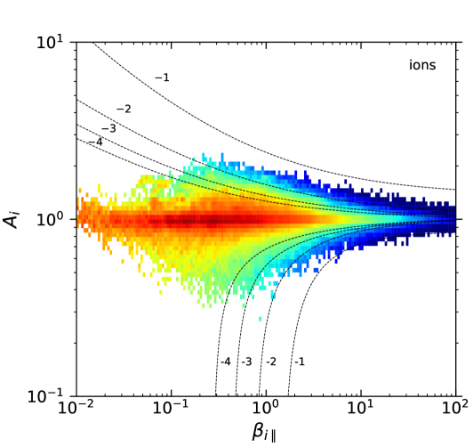


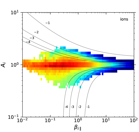
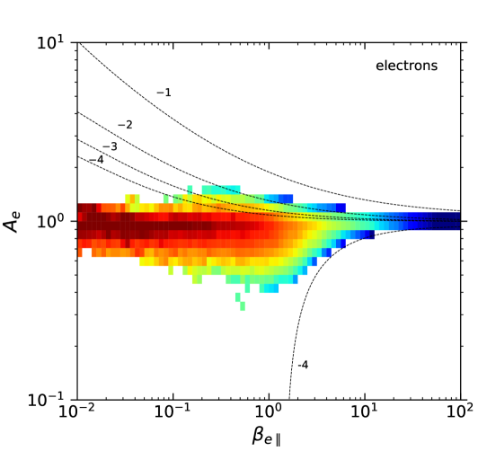
In total, for the ions it was possible to calculate 576,954 magnetic fluctuations with their respective and values. For the electrons the total number of detections was similar: 569,450 magnetic fluctuations with and values. Fig. 1 shows the probability density of the available measurements for each value of and , for both ions and electrons. This probability was calculated as the number of available measurements in a given bin divided by the total number of measurements for the particular species, and divided by the area of the bin (which is variable due to the logarithmic scale). The top two panels in the figure were divided in cells of sizes (in a log-log scale) and each box was colored only if . Similarly, the bottom two panels were divided in cells of sizes and colored only if . Let us note that the change in threshold value between the two cases is consistent with an approximate increase by of factor of 4 in the number of measurements when going from a cell size of to in log-log space. We further confirmed (not shown here) that these thresholds provide a consistent behavior when re-sampling the data into smaller sets with a third of the data points. Thus, we use a cell size of with a threshold value of in all other diagrams below.
The event probability patterns shown in Fig. 1(top) for each species are consistent with observations in the magnetosheath by the CLUSTER (Gary et al., 2005), AMPTE (Phan et al., 1994; Anderson et al., 1994), and MMS missions (Maruca et al., 2018); as well as in the solar wind (Gary et al., 2001a; Hellinger et al., 2006; Štverák et al., 2008; Adrian et al., 2016; Huang et al., 2020), computer simulations (Gary et al., 2001b; Yoon & Seough, 2012), and laboratory experiments (Scime et al., 2015, 2000; Beatty et al., 2020)
A key difference with most of these works is that the particle energy distributions for ions and electrons in the plasma sheet are better fitted by Kappa distributions (Espinoza et al., 2018; Eyelade et al., 2021), and that the ion temperature anisotropy is restricted to values ; whereas in the solar wind the ion velocity distributions are mostly Maxwellians with temperature anisotropies in the range . On the other hand, the electron anisotropy distribution in the plasma sheet, as shown in Fig. 1, is similar to that observed for core and halo electrons in the solar wind (Štverák et al., 2008).
In Fig. 2, we display the observed parallel () and perpendicular (, known as magnetic compressibility) fluctuation levels, as defined by Eqs. (1) and (2), respectively. We also show the total observed magnetic fluctuations (), for which high activity is observed even for , where one would (naively, from a linear description) not expect significant fluctuations. We think that a relevant component of the observed fluctuations can be thermally induced, as suggested by Navarro et al. (2014a). To test such prediction for the magnetospheric environment we compare our THEMIS observations with the theory of spontaneous magnetic fluctuations outlined in Section 4.
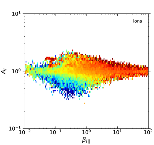
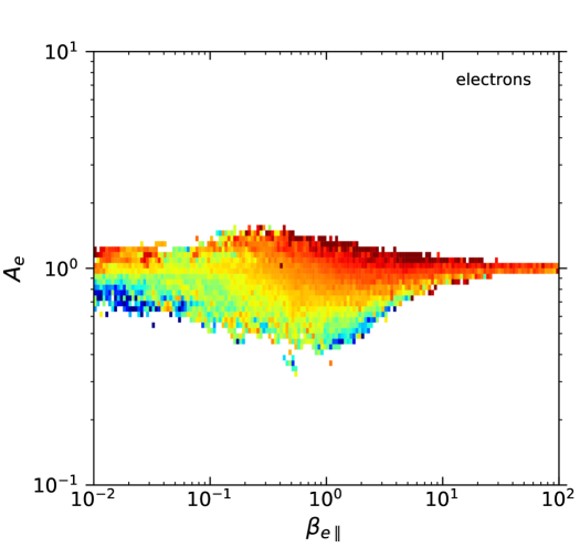
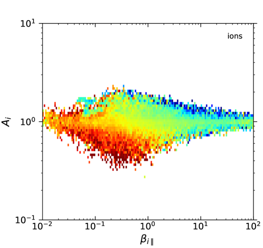
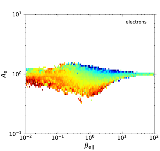
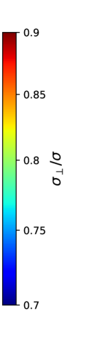
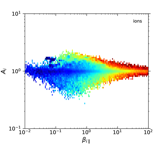
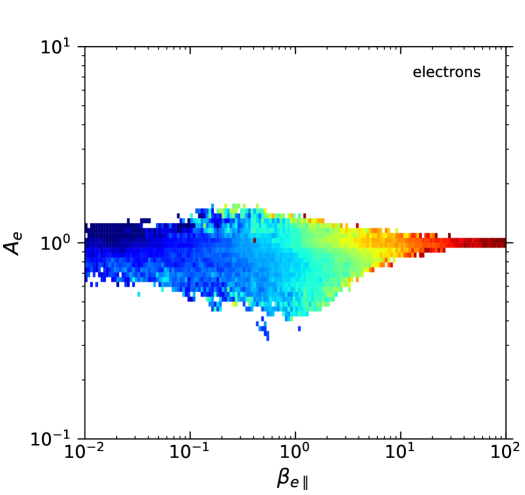
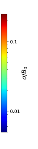
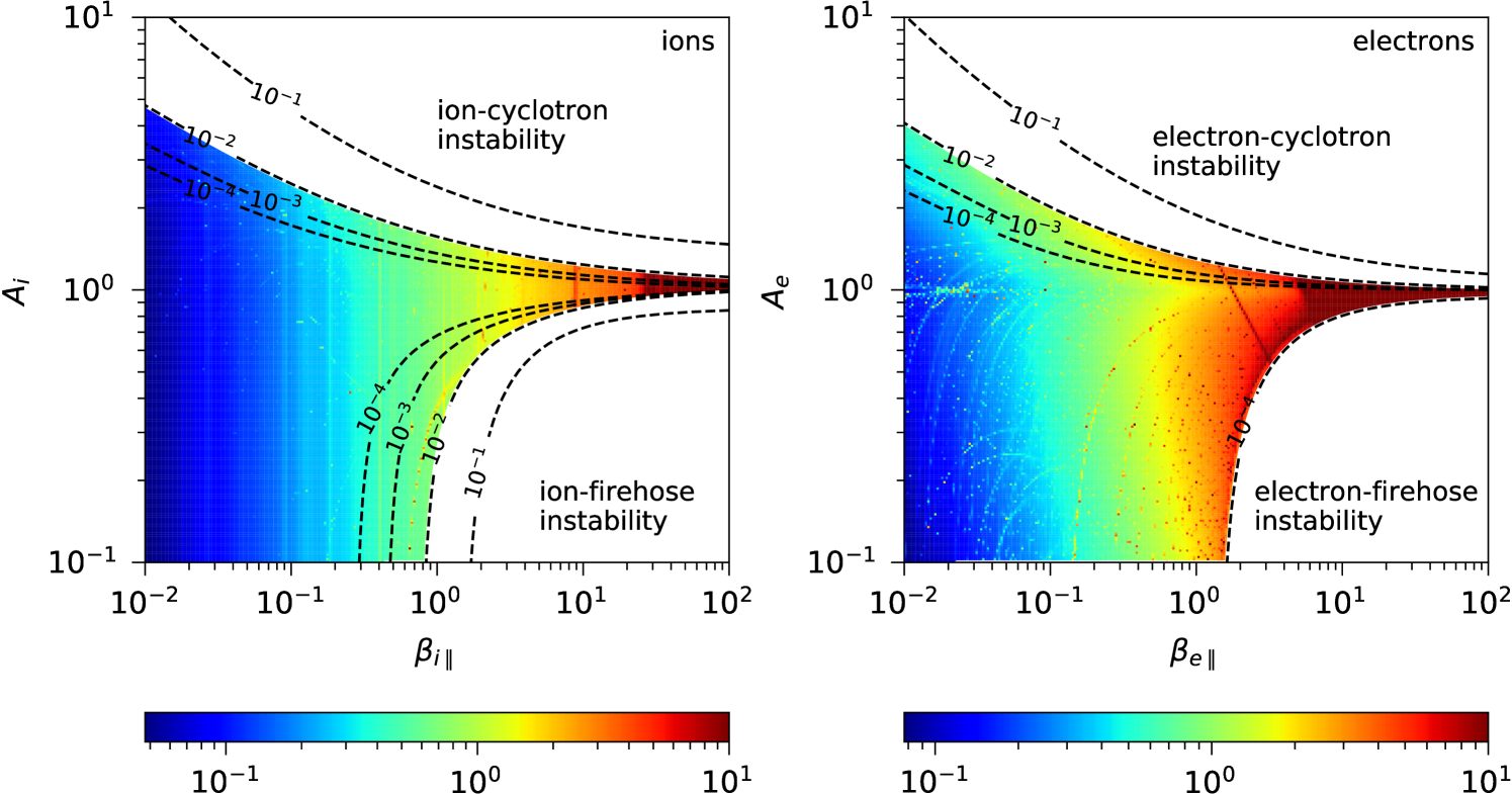
Figure 3 shows computed from Eq. (12) as a function of and for ions and electrons. It was assumed that , , and , as suggested by Espinoza et al. (2018). For fluctuations at the ion scales, we assumed that the electron anisotropy effects are negligible, for which we set . Similarly, we set for fluctuations at the electron scales. The segmented lines in Figs. 3 and 1 are the contours of the maximum growth-rate of the instabilities listed in Tables 1 and 2. The pattern of in the - diagrams in Fig. 3 can be compared with the observed magnetic fluctuations shown in Fig. 2 (bottom) as a function of the proton and electron parameters. The trending on the magnetic fluctuations increases mainly with , and to some extent with .
6 Discussion
Although the total magnetic power in thermally induced electromagnetic fluctuations (calculated from Eq. (12) and shown in Fig. 3) is in arbitrary units, it resembles qualitatively well the patterns on the observed diagrams (obtained from THEMIS data and plotted in Fig. 2), thereby suggesting that such fluctuations may constitute a relevant component of the turbulence observed. The similarity of these results with those obtained for the solar wind (Navarro et al., 2014b) suggests that the kinetic physics plays an important role in the regulation of plasma turbulence and generation of fluctuations, in both the solar wind and the plasma sheet.
Figure 1 shows that the majority of measurements lie far from the instability thresholds listed in Tables 1 and 2. In particular, the ion-cyclotron (Alfvén) instability with values of appears as an upper bound to the observable conditions for ; while the electron-anisotropy seems to be constrained by the electron-cyclotron (whistler) instability with (or if normalized to the ion gyrofrequency). Thus, the anisotropy of both species for seems to be constrained by approximately the same level (relative to the species scale) of the respective resonant instability. We acknowledge that this deserves further study. Of course, other instability rates would appear to represent the observations if a different threshold was used. What matters is that the dependency on of both observations and theory are similar, which suggests that the kinetic instabilities could indeed regulate the global behavior of the observations, hence of the turbulence.
Similarly, the electron temperature anisotropy seems to be constrained by a much lower level of the (non-resonant) electron-firehose instability compared with , with . For ions, it is not clear if a similar statement is true. While is indeed constrained by the (non-resonant) ion-firehose instability with , this seems to apply only for high values. For other effects that were not considered here may affect the growth-rate levels. For instance, other values of the indexes (Navarro et al., 2015) and the presence of anisotropic electrons can affect the development of ion-firehose instabilities (Michno et al., 2014; Maneva et al., 2016).
Let us note that the approximation of parallel propagation is quite reasonable, since for most of the observed and values, for both ions and electrons (Fig. 2, top). This is consistent with the propagation of non-compressive fluctuations (i.e. transverse ion- or electron-cyclotron waves propagating along the background magnetic field).
7 Conclusions
We have shown that temperature anisotropy at the kinetic level can regulate turbulence in the plasma sheet of the geomagnetic tail. Similar results have been obtained for the solar wind (Bale et al., 2009) and the magnetosheath (e.g. Maruca et al., 2018), and we conclude that this behavior might be more universal than previously expected. Furthermore, our results also suggest that physics at the kinetic level may be a relevant contributor to the magnetic fluctuations observed in these plasmas. We demonstrated that the resonant Alfvén and whistler instabilities may regulate the observed anisotropies for values above unity. Electron anisotropies seem to be constrained by the non-resonant firehose instability, while for ion anisotropies this statement is still not clear. The ion and electron cyclotron instabilities seem to operate on time scales comparable to the scales of protons or electrons. This does not seem to be the case for the firehose instabilities, so that more work and precise measurements are needed to understand these results.
In both the solar wind and the plasma sheet, the plasma appear to converge to a common dynamic quasi-equilibrium state. Understanding this universality may have implications for other astrophysical and laboratory plasma environments (López et al., 2015). Therefore, spontaneous fluctuations and their collisionless kinetic regulation may be fundamental features of space and astrophysical plasmas. Furthermore, this is a topic of current scientific interest, not only because of the need to advance our quantitative understanding of kinetic effects in the regulation of turbulence and production of electromagnetic fluctuations; but also because of its possible impact on the development of robust and accurate space weather forecasts during geomagnetic storms and substorms, where plasma turbulence and electromagnetic fluctuations seem to play a substantial role (e.g. Borovsky & Funsten, 2003; Klimas et al., 2000; Sitnov et al., 2000; Valdivia et al., 2003; Stepanova et al., 2009; Stepanova & Antonova, 2011; Stepanova et al., 2011; Pinto et al., 2011; Valdivia et al., 2016; Antonova & Stepanova, 2021). Moreover, as Navarro et al. (2014b), we suggest that it may be possible to relate the thermal properties of the particle distribution functions with the production of magnetic fluctuations, a result that may position us one step closer to understand turbulent behavior in plasmas.
THEMIS
References
- Adrian et al. (2016) Adrian, M. L., Viñas, A. F., Moya, P. S., & Wendel, D. E. 2016, The Astrophysical Journal, 833, 49, doi: 10.3847/1538-4357/833/1/49
- Anderson et al. (1994) Anderson, B. J., Fuselier, S. A., Gary, S. P., & Denton, R. E. 1994, J. Geophys. Res., 99, 5877, doi: https://doi.org/10.1029/93JA02827
- Angelopoulos (2008) Angelopoulos, V. 2008, Space Sci. Rev., 141, 5, doi: 10.1007/s11214-008-9336-1
- Angelopoulos et al. (1993) Angelopoulos, V., Kennel, C. F., Coroniti, F. V., et al. 1993, Geophysical Research Letters, 20, 1711, doi: 10.1029/93GL00847
- Antonova & Ovchinnikov (1999) Antonova, E. E., & Ovchinnikov, I. L. 1999, Journal of Geophysical Research, 104, 17289, doi: 10.1029/1999JA900141
- Antonova & Stepanova (2021) Antonova, E. E., & Stepanova, M. V. 2021, Frontiers in Astronomy and Space Sciences, 8, 26, doi: 10.3389/fspas.2021.622570
- Araneda et al. (2012) Araneda, J. A., Astudillo, H., & Marsch, E. 2012, Space Sci. Rev., 172, 361, doi: 10.1007/s11214-011-9773-0
- Auster et al. (2008) Auster, H. U., Glassmeier, K. H., Magnes, W., et al. 2008, Space Sci. Rev., 141, 235, doi: 10.1007/s11214-008-9365-9
- Bale et al. (2009) Bale, S. D., Kasper, J. C., Howes, G. G., et al. 2009, Physical Review Letters, 103, 211101, doi: 10.1103/PhysRevLett.103.211101
- Beatty et al. (2020) Beatty, C. B., Steinberger, T. E., Aguirre, E. M., et al. 2020, Phys. Plasmas, 27, 122101, doi: 10.1063/5.0029315
- Borovsky et al. (1997) Borovsky, J. E., Elphic, R. C., Funsten, H. O., & Thomsen, M. F. 1997, Journal of Plasma Physics, 57, 1, doi: 10.1017/S0022377896005259
- Borovsky & Funsten (2003) Borovsky, J. E., & Funsten, H. O. 2003, Journal of Geophysical Research (Space Physics), 108, 1284, doi: 10.1029/2002JA009625
- Borovsky et al. (2020) Borovsky, J. E., Delzanno, G. L., Valdivia, J. A., et al. 2020, Journal of Atmospheric and Solar-Terrestrial Physics, 208, 105377, doi: 10.1016/j.jastp.2020.105377
- Denton et al. (2016) Denton, M. H., Borovsky, J. E., Stepanova, M., & Valdivia, J. A. 2016, Journal of Geophysical Research (Space Physics), 121, 10,783, doi: 10.1002/2016JA023362
- Espinoza et al. (2018) Espinoza, C. M., Stepanova, M., Moya, P. S., Antonova, E. E., & Valdivia, J. A. 2018, Geophysical Research Letters, 45, 6362, doi: 10.1029/2018GL078631
- Eyelade et al. (2021) Eyelade, A. V., Stepanova, M., Espinoza, C. M., & Moya, P. S. 2021, Astrophys. J. Suppl. S., 253, 34, doi: 10.3847/1538-4365/abdec9
- Gary et al. (2005) Gary, S. P., Lavraud, B., Thomsen, M. F., Lefebvre, B., & Schwartz, S. J. 2005, Geophys. Res. Lett., 32, doi: https://doi.org/10.1029/2005GL023234
- Gary et al. (2001a) Gary, S. P., Skoug, R. M., Steinberg, J. T., & Smith, C. W. 2001a, Geophys. Res. Lett., 28, 2759, doi: https://doi.org/10.1029/2001GL013165
- Gary et al. (2001b) Gary, S. P., Yin, L., Winske, D., & Ofman, L. 2001b, J. Geophys. Res., 106, 10715, doi: https://doi.org/10.1029/2000JA000406
- Hellberg & Mace (2002) Hellberg, M. A., & Mace, R. L. 2002, Physics of Plasmas, 9, 1495, doi: 10.1063/1.1462636
- Hellinger et al. (2006) Hellinger, P., Trávníček, P., Kasper, J. C., & Lazarus, A. J. 2006, Geophysical Research Letters, 33, L09101, doi: 10.1029/2006GL025925
- Huang et al. (2020) Huang, J., Kasper, J. C., Vech, D., et al. 2020, Astrophys. J. Suppl. Ser., 246, 70, doi: 10.3847/1538-4365/ab74e0
- Isenberg et al. (2013) Isenberg, P. A., Maruca, B. A., & Kasper, J. C. 2013, ApJ, 773, 164, doi: 10.1088/0004-637X/773/2/164
- Kasper et al. (2006) Kasper, J. C., Lazarus, A. J., Steinberg, J. T., Ogilvie, K. W., & Szabo, A. 2006, J. Geophys. Res., 111, A03105, doi: https://doi.org/10.1029/2005JA011442
- Klimas et al. (2000) Klimas, A. J., Valdivia, J. A., Vassiliadis, D., et al. 2000, Journal of Geophysical Research, 105, 18,765, doi: 10.1029/1999JA000319
- López et al. (2015) López, R. A., Navarro, R. E., Moya, P. S., et al. 2015, ApJ, 810, 103, doi: 10.1088/0004-637X/810/2/103
- Maneva et al. (2016) Maneva, Y., Lazar, M., Viñas, A., & Poedts, S. 2016, The Astrophysical Journal, 832, 64, doi: 10.3847/0004-637x/832/1/64
- Maruca et al. (2011) Maruca, B. A., Kasper, J. C., & Bale, S. D. 2011, Physical Review Letters, 107, 201101, doi: 10.1103/PhysRevLett.107.201101
- Maruca et al. (2018) Maruca, B. A., Chasapis, A., Gary, S. P., et al. 2018, The Astrophysical Journal, 866, 25, doi: 10.3847/1538-4357/aaddfb
- McFadden et al. (2008) McFadden, J., Carlson, C., Larson, D., et al. 2008, Space Science Reviews, 141, 277, doi: 10.1007/s11214-008-9440-2
- Michno et al. (2014) Michno, M. J., Lazar, M., Yoon, P. H., & Schlickeiser, R. 2014, The Astrophysical Journal, 781, 49, doi: 10.1088/0004-637x/781/1/49
- Moya et al. (2020) Moya, P. S., Lazar, M., & Poedts, S. 2020, Plasma Physics and Controlled Fusion, 63, 025011, doi: 10.1088/1361-6587/abce1a
- Moya & Navarro (2021) Moya, P. S., & Navarro, R. E. 2021, Frontiers in Physics, 9, 175, doi: 10.3389/fphy.2021.624748
- Navarro et al. (2014a) Navarro, R., Araneda, J., Muñoz, V., et al. 2014a, Physics of Plasmas, 21, 092902, doi: 10.1063/1.4894700
- Navarro et al. (2014b) Navarro, R., Moya, P., Muñoz, V., et al. 2014b, Physical Review Letters, 112, 245001, doi: 10.1103/PhysRevLett.112.245001
- Navarro et al. (2015) Navarro, R. E., Moya, P. S., Muñoz, V., et al. 2015, Journal of Geophysical Research (Space Physics), 120, 2382, doi: 10.1002/2014JA020550
- Ovchinnikov et al. (2000) Ovchinnikov, I. L., Antonova, E. E., & Yermolaev, Y. I. 2000, Cosmic Research, 38, 557, doi: 10.1023/A:1026686600686
- Phan et al. (1994) Phan, T. D., Paschmann, G., Baumjohann, W., Sckopke, N., & Lühr, H. 1994, J. Geophys. Res., 99, 121, doi: https://doi.org/10.1029/93JA02444
- Pinto et al. (2011) Pinto, V., Stepanova, M., Antonova, E. E., & Valdivia, J. A. 2011, Journal of Atmospheric and Solar-Terrestrial Physics, 73, 1472, doi: 10.1016/j.jastp.2011.05.007
- Scime et al. (2000) Scime, E. E., Keiter, P. A., Balkey, M. M., et al. 2000, Phys. Plasmas, 7, 2157, doi: 10.1063/1.874036
- Scime et al. (2015) —. 2015, J. Plasma Phys., 81, 345810103, doi: 10.1017/S0022377814000890
- Sitnov et al. (2000) Sitnov, M. I., Zelenyi, L. M., Malova, H. V., & Sharma, A. S. 2000, Journal of Geophysical Research, 105, 13029, doi: 10.1029/1999JA000431
- Stepanova & Antonova (2011) Stepanova, M., & Antonova, E. E. 2011, Journal of Atmospheric and Solar-Terrestrial Physics, 73, 1636, doi: 10.1016/j.jastp.2011.02.009
- Stepanova et al. (2009) Stepanova, M., Antonova, E. E., Paredes-Davis, D., Ovchinnikov, I. L., & Yermolaev, Y. I. 2009, Annales Geophysicae, 27, 1407, doi: 10.5194/angeo-27-1407-2009
- Stepanova et al. (2011) Stepanova, M., Pinto, V., Valdivia, J. A., & Antonova, E. E. 2011, Journal of Geophysical Research (Space Physics), 116, 0, doi: 10.1029/2010JA015887
- Summers & Thorne (1991) Summers, D., & Thorne, R. M. 1991, Physics of Fluids B: Plasma Physics, 3, 1835, doi: 10.1063/1.859653
- Valdivia et al. (2003) Valdivia, J. A., Klimas, A., Vassiliadis, D., Uritsky, V., & Takalo, J. 2003, Space Science Reviews, 107, 515, doi: 10.1023/A:1025518527128
- Valdivia et al. (2016) Valdivia, J. A., Toledo, B. A., Gallo, N., et al. 2016, Advances in Space Research, 58, 2126, doi: 10.1016/j.asr.2016.04.017
- Viñas et al. (2015) Viñas, A. F., Moya, P. S., Navarro, R. E., et al. 2015, Journal of Geophysical Research (Space Physics), 120, 3307, doi: 10.1002/2014JA020554
- Viñas et al. (2017) Viñas, A. F., Gaelzer, R., Moya, P. S., Mace, R., & Araneda, J. A. 2017, in Kappa Distributions, ed. G. Livadiotis (Elsevier), 329–361, doi: 10.1016/B978-0-12-804638-8.00007-3
- Volwerk et al. (2004) Volwerk, M., Vörös, Z., Baumjohann, W., et al. 2004, Annales Geophysicae, 22, 2525, doi: 10.5194/angeo-22-2525-2004
- Vörös et al. (2004) Vörös, Z., Baumjohann, W., Nakamura, R., et al. 2004, Journal of Geophysical Research (Space Physics), 109, A11215, doi: 10.1029/2004JA010404
- Štverák et al. (2008) Štverák, v., Trávníček, P., Maksimovic, M., et al. 2008, J. Geophys. Res., 113, A03103, doi: https://doi.org/10.1029/2007JA012733
- Weygand et al. (2005) Weygand, J. M., Kivelson, M. G., Khurana, K. K., et al. 2005, Journal of Geophysical Research (Space Physics), 110, A01205, doi: 10.1029/2004JA010581
- Yoon & Seough (2012) Yoon, P. H., & Seough, J. 2012, J. Geophys. Res., 117, doi: https://doi.org/10.1029/2012JA017697
- Yue et al. (2016) Yue, C., An, X., Bortnik, J., et al. 2016, Geophysical Research Letters, 43, 7804, doi: https://doi.org/10.1002/2016GL070084