Spontaneous Scalarization in Scalar-Tensor Theories with Conformal Symmetry as an Attractor

We consider scalar-tensor theories of gravity whose action in the Jordan frame is given by

$\displaystyle S=\int d^{4}x\sqrt{-g}\frac{1}{16\pi}\left(\Phi R-\frac{\omega({\Phi})}{{\Phi}}(\nabla{\Phi})^{2}\right)+S_{M}(\psi,g_{\mu\nu})\,,$

(2)

where ${\Phi}$ is the so-called Brans-Dicke scalar field, the inverse of which plays the role of the effective gravitational “constant”, $\omega({\Phi})$ is the Brans-Dicke function which determines the strength of the coupling of the scalar field to gravity (and matter), $S_{M}$ is the matter action and $\psi$ denotes the matter field.

We note that for $\omega=-3/2$, the gravity part of the action is locally conformal invariant under the following Weyl scaling²²2The action is still conformal invariant even if one includes a potential proportional to ${\Phi}^{2}$. However, the equation of the motion of the scalar field is not affected by such a potential as discussed in 2.2. :

$\displaystyle g_{\mu\nu}\rightarrow e^{2\sigma(x)}g_{\mu\nu},~{}~{}~{}~{}~{}{\Phi}\rightarrow e^{-2\sigma(x)}{\Phi}\,.$

(3)

From the post-Newtonian expansion of the theory, the effective gravitational constant $G$ and the parametrized post-Newtonian (PPN) parameters $\gamma$ and $\beta$ of scalar-tensor theories are given by will2018 ³³3We do not use the units of the present-day gravitational constant $G=1$ at this stage because we are interested in the cosmological evolution of ${\Phi}$.

	$\displaystyle G$	$\displaystyle=$	$\displaystyle\frac{1}{{\Phi}}\frac{2\omega({\Phi})+4}{2\omega({\Phi})+3}\bigg{|}_{{\Phi}_{0}}$		(4)
	$\displaystyle\gamma$	$\displaystyle=$	$\displaystyle\frac{\omega+1}{\omega+2}\,,$		(5)
	$\displaystyle\beta$	$\displaystyle=$	$\displaystyle 1+\frac{{\Phi}\frac{d\omega}{d{\Phi}}}{4(2\omega+3)(\omega+2)^{2}}\,.$		(6)

The equation of motion of a massive body is given in Damour:1992we ; will2018 . It contains terms which depend on the gravitational self-energy, the coefficient of which is $\eta=4\beta-\gamma-3$. For $\eta=0$, the motion of massive bodies does not depend on their internal structure and hence respects SEP.

Remarkably, $\eta$ and $G$ are related by (see Damour:1992we for a similar relation)

$\displaystyle\eta=(\gamma-1)\frac{d\ln G}{d\ln{\Phi}}.$

(7)

Therefore, $\eta=0$, for which the theory respects the SEP, implies either $\gamma=1$ (GR) or $G={\rm const}$. The latter is known as “constant-$G$” theory found by Barker 1978ApJ…219….5B in which $\omega({\Phi})$ is given by

$\displaystyle\omega({\Phi})=-\frac{3}{2}+\frac{1}{2G{\Phi}-2}$

(8)

Note that $|\omega|\rightarrow\infty$ (GR) for $G{\Phi}\rightarrow 1$ and that $\omega\rightarrow-3/2$ (conformal symmetry) for $G|{\Phi}|\rightarrow\infty$. The constraint on $\gamma$ from the measurement of the time delay of the Cassini spacecraft is $\gamma-1=(2.1\pm 2.3)\times 10^{-5}$ Bertotti:2003rm , which is satisfied for $G{\Phi}-1=(-1.1\pm 1.2)\times 10^{-6}$ at present.

In order to study the dynamics of ${\Phi}$, it is useful to perform the following change of variables and moving to the so-called Einstein frame Damour:1993id ; Chiba:2013mha in which ${\Phi}$ is decoupled from the gravity sector:

	$\displaystyle g_{\mu\nu}$	$\displaystyle=$	$\displaystyle\frac{1}{G_{*}{\Phi}}\overline{g}_{\mu\nu}\equiv e^{2a({\varphi})}\overline{g}_{\mu\nu}$		(9)
	$\displaystyle\frac{1}{2\omega+3}$	$\displaystyle=$	$\displaystyle\frac{1}{4\pi G_{*}}\left(\frac{da({\varphi})}{d{\varphi}}\right)^{2}\equiv\frac{1}{4\pi G_{*}}\alpha({\varphi})^{2}$		(10)

where $G_{*}$ is the bare gravitational constant. The action (2) can be rewritten in terms of $\overline{g}_{{\mu}{\nu}}$ whose kinetic term is of Einstein-Hilbert form and a canonically normalized scalar field ${\varphi}$ as ⁴⁴4 Note that our ${\varphi}$ is related to the scalar field in Damour:1992we ; Damour:1993hw ${\varphi}_{\rm DEF}$ via ${\varphi}_{\rm DEF}=\kappa{\varphi}/\sqrt{2}$.

$\displaystyle S=\int d^{4}x\sqrt{-\overline{g}}\left(\frac{\bar{R}}{16\pi G_{*}}-\frac{1}{2}(\overline{\nabla}{\varphi})^{2}\right)+S_{M}(\psi,e^{2a}\overline{g}_{\mu\nu})$

(11)

From Eq. (11), the equation of motion of $\overline{g}_{{\mu}{\nu}}$ and ${\varphi}$ are given by

	$\displaystyle{\overline{R}}_{{\mu}{\nu}}-\frac{1}{2}\overline{g}_{{\mu}{\nu}}{\overline{R}}=8\pi G_{*}\left({\overline{T}}_{{\mu}{\nu}}+\partial_{{\mu}}{\varphi}\partial_{{\nu}}{\varphi}-\frac{1}{2}\overline{g}_{{\mu}{\nu}}(\overline{\nabla}{\varphi})^{2}\right)$		(12)
	$\displaystyle\overline{\Box}{\varphi}=-\alpha({\varphi}){\overline{T}}$		(13)

where ${\overline{T}}_{{\mu}{\nu}}=-(2/\sqrt{-\overline{g}})\delta S_{M}/\delta\overline{g}^{{\mu}{\nu}}$ is the energy-momentum tensor in the Einstein frame. From Eq. (13), we find that ${\varphi}$ moves according to the effective potential $-a({\varphi}){\overline{T}}$.⁵⁵5We note that the action Eq.(2) is still conformal invariant even if one includes a potential proportional to ${\Phi}^{2}$. In the Einstein frame action Eq.(11) such a potential corresponds to a constant and does not affect the evolution of the scalar field. The effective gravitational constant $G$ and the PPN parameter $\gamma$ are written as

	$\displaystyle G$	$\displaystyle=$	$\displaystyle G_{*}e^{2a({\varphi})}\left(1+2\alpha({\varphi})^{2}/\kappa^{2}\right)\bigg{|}_{{\varphi}_{0}}$		(14)
	$\displaystyle\gamma-1$	$\displaystyle=$	$\displaystyle-\frac{4\alpha({\varphi})^{2}/\kappa^{2}}{2\alpha({\varphi})^{2}/\kappa^{2}+1}\bigg{|}_{{\varphi}_{0}}$		(15)

where $\kappa=\sqrt{8\pi G_{*}}$ and ${\varphi}_{0}$ denotes the value of ${\varphi}$ at spatial infinity.

For constant-$G$ theory with $\omega({\Phi})$ in Eq. (8), from Eq. (9) and Eq. (10), ${\varphi}$ and $a({\varphi})$ are given by

	$\displaystyle\kappa{\varphi}$	$\displaystyle=$	$\displaystyle\sqrt{2}\tan^{-1}\sqrt{G{\Phi}-1}$		(16)
	$\displaystyle a({\varphi})$	$\displaystyle=$	$\displaystyle\ln\left(\cos\left(\kappa{\varphi}/\sqrt{2}\right)\right)$		(17)

where $G{\Phi}\geq 1$ is assumed ($\cosh$ for $G{\Phi}<1$) and $G_{*}$ coincides with $G$. We have fixed the integration constant so that $G{\Phi}=1$ corresponds to $\kappa{\varphi}=0$. The conformal symmetry ($G{\Phi}\rightarrow\infty$) now corresponds to $\kappa{\varphi}\rightarrow\pi/\sqrt{2}$. In Fig. 1, $a({\varphi})$ is shown. The constraint by the Cassini experiment is satisfied for $\kappa{\varphi}=(-2.6\pm 4.0)\times 10^{-3}$ at present. From Eq. (13), one may see that ${\varphi}$ moves toward $\kappa{\varphi}\rightarrow\pi/\sqrt{2}$ according to the effective potential $-a({\varphi}){\overline{T}}$ (see Fig. 1) during the matter-dominated epoch and during the dark energy-dominated epoch: The theory is thus cosmologically attracted toward the conformal symmetry Gerard:2006ia .

Although the scalar-tensor theory with $\eta=0$ is unique, we may consider possible generalization of the models which exhibit cosmological attraction toward the conformal symmetry.

For example, we can consider the following generalization of the coupling function $a({\varphi})$ in Eq. (17):

$\displaystyle a({\varphi})=\ln\left(\cos\left(\sqrt{p}~{}\kappa{\varphi}\right)\right)$

(18)

where $p$ is a non-negative parameter and $p=1/2$ corresponds to constant-G theory. From Eq. (9) and Eq. (10), the corresponding ${\Phi}$ and $\omega({\Phi})$ are given by

	$\displaystyle G_{*}{\Phi}$	$\displaystyle=$	$\displaystyle\sec^{2}(\sqrt{p}~{}\kappa{\varphi})$		(19)
	$\displaystyle\omega({\Phi})$	$\displaystyle=$	$\displaystyle-\frac{3}{2}+\frac{1}{4p}\frac{1}{G_{*}{\Phi}-1}\,.$		(20)

The conformal symmetry $\omega=-3/2$ now corresponds to $\kappa{\varphi}=\pi/(2\sqrt{p})$ and the shape of $a({\varphi})$ is similar to Eq. (17) ($p=1/2$) and we expect similar cosmological attraction toward the conformal symmetry. ⁶⁶6We note that a theory with a quadratic function $a({\varphi})=-\frac{1}{2}p(\kappa{\varphi})^{2}$ with $p>0$ Damour:1993hw is also cosmologically attracted toward the conformal symmetry.

On the other hand, the effective gravitational constant $G$ defined by Eq. (4) is given by

$\displaystyle G=2pG_{*}+\frac{1-2p}{{\Phi}},$

(21)

and the gravitational constant is no longer constant. PPN parameters $\gamma$ and $\beta$ and $\eta=4\beta-\gamma-3$ are given from Eq.(5) and Eq. (6) by

	$\displaystyle\gamma-1$	$\displaystyle=$	$\displaystyle-\frac{4p(G_{*}{\Phi}-1)}{2pG_{*}{\Phi}+1-2p}$		(22)
	$\displaystyle\beta-1$	$\displaystyle=$	$\displaystyle-\frac{2p^{2}G_{*}{\Phi}(G_{*}{\Phi}-1)}{(2pG_{*}{\Phi}+1-2p)^{2}}$		(23)
	$\displaystyle\eta$	$\displaystyle=$	$\displaystyle-\frac{4p(2p-1)(G_{*}{\Phi}-1)}{(2pG_{*}{\Phi}+1-2p)^{2}}.$		(24)

In terms of $\gamma$, $\eta$ can be rewritten in a suggestive form:

$\displaystyle\eta=(2p-1)\left(\frac{\gamma+1}{2}\right)(\gamma-1).$

(25)

Therefore, although $\eta$ is no longer vanishing as long as $p\neq 1/2$, it is suppressed by $\gamma-1$. From the bound by Cassini $\gamma-1=(2.1\pm 2.3)\times 10^{-5}$ Bertotti:2003rm , the constraint on $\eta$ from the lunar-laser-ranging experiment, $\eta=(-0.2\pm 1.1)\times 10^{-4}$ Hofmann:2018myc , is satisfied for $p<2.9$.

We study the spherically symmetric static solutions generated by perfect fluid neutron stars in scalar-tensor theories. The metric in the Einstein frame is assumed to be of the form

$\displaystyle\overline{g}_{{\mu}{\nu}}dx^{\mu}dx^{\nu}=-e^{\nu(r)}dt^{2}+\frac{dr^{2}}{1-2\mu(r)/r}+r^{2}d\Omega^{2}\,.$

(26)

The perfect fluid energy-momentum in the Jordan frame is

$\displaystyle T^{\mu\nu}=(\epsilon+p)u^{\mu}u^{\nu}+pg^{\mu\nu}$

(27)

and is related to the energy-momentum tensor in the Einstein frame by ${{\bar{T}}^{\mu}}_{~{}~{}\nu}=e^{4a}{T^{\mu}}_{\nu}$. The equation of motion Eq. (12) and Eq. (13) become

	$\displaystyle\mu^{\prime}$	$\displaystyle=$	$\displaystyle 4\pi G_{*}r^{2}e^{4a({\varphi})}\epsilon+2\pi G_{*}r(r-2\mu){\varphi}^{\prime 2}$		(28)
	$\displaystyle\nu^{\prime}$	$\displaystyle=$	$\displaystyle\frac{2\mu}{r(r-2\mu)}+8\pi G_{*}\frac{r^{2}e^{4a({\varphi})}}{r-2\mu}p+4\pi G_{*}r{\varphi}^{\prime 2}$		(29)
	$\displaystyle{\varphi}^{\prime\prime}$	$\displaystyle=$	$\displaystyle-\frac{2(r-\mu)}{r(r-2\mu)}{\varphi}^{\prime}+4\pi G_{*}\frac{r^{2}e^{4a({\varphi})}}{r-2\mu}(\epsilon-p){\varphi}^{\prime}+\frac{re^{4a({\varphi})}}{r-2\mu}(\epsilon-3p)\alpha({\varphi})$		(30)
	$\displaystyle p^{\prime}$	$\displaystyle=$	$\displaystyle-(\epsilon+p)\left(\frac{\mu}{r(r-2\mu)}+4\pi G_{*}\frac{r^{2}e^{4a({\varphi})}}{r-2\mu}p+2\pi G_{*}r{\varphi}^{\prime 2}+\alpha({\varphi}){\varphi}^{\prime}\right)$		(31)

where the prime denotes a derivative with respect to $r$.

With the coupling function $a({\varphi})$ Eq. (18), given the initial conditions at $r=0$, we numerically integrate these equation outward using a 4th-order Runge-Kutta method. The pressure goes to zero at the surface of star, and beyond that only the metric and scalar equations with vanishing $p$ and $\epsilon$ are necessary. Specifically, we set $p$ and $\epsilon$ to zero if $p$ is less than $10^{-7}m_{B}n_{0}$ (with $m_{B}=1.66\times 10^{-24}{\rm g}$ and $n_{0}=0.1{\rm fm}^{-3}$) well below neutron drip and integrate Eq. (28) $\sim$ Eq. (30) further outward. The regularity at $r=0$ requires $\mu(0)=\nu(0)={\varphi}^{\prime}(0)=0$. We can freely specify ${\varphi}(0)$ and $p(0)$. But in order to satisfy the bound by the Cassini satellite experiment $|\gamma-1|<2.3\times 10^{-5}$, from Eq. (15) the asymptotic value ${\varphi}_{0}$ should satisfy $\alpha({\varphi}_{0})/\kappa<2.4\times 10^{-3}$. Considering the limit on $\gamma$ and in order to put conservative constraints on the theory, we require $\alpha({\varphi}_{0})/\kappa=1.0\times 10^{-4}$ at large $r$. Hence, for a given $p(0)$, a particular value of ${\varphi}(0)$ can satisfy this condition. We employ the shooting method to find ${\varphi}(0)$.

As an equation of state (EOS), we adopt piecewise-polytropic parametrizations for the nuclear EOS by Read et al. Read:2008iy for APR4 Akmal:1998cf and H4 Glendenning:1991es ; Lackey:2005tk and MS1 Mueller:1996pm EOSs. APR4 (variational method) and MS1 (relativistic mean-field theory) are EOSs for nuclear matter composed of neutrons, protons, electrons, and muons, whereas H4 (relativistic mean-field theory) includes the effect of hyperons in addition.

A piecewise polytropic EOS consists of several polytropic EOSs

$\displaystyle p(\rho)=K_{i}\rho^{\Gamma_{i}},~{}~{}~{}~{}~{}~{}\rho_{i-1}\leq\rho\leq\rho_{i},$

(32)

where $\rho$ is the rest-mass density. From the continuity of the pressure at $\rho_{i}$ determines $K_{i+1}$ at the next interval as $K_{i+1}={p(\rho_{i})}/{\rho_{i}^{\Gamma_{i+1}}}$. The energy density $\epsilon$ is determined by the first law of thermodynamics, $d(\epsilon/\rho)=-pd(1/\rho)$ as

$\displaystyle\epsilon=(1+a_{i})\rho+\frac{K_{i}}{\Gamma_{i}-1}\rho^{\Gamma_{i}},~{}~{}~{}~{}~{}\rho_{i-1}\leq\rho\leq\rho_{i},$

(33)

where $a_{i}$ is an integration constant given by

$\displaystyle a_{i}=\frac{\epsilon(\rho_{i-1})}{\rho_{i-1}}-1-\frac{K_{i-1}}{\Gamma_{i}-1}\rho_{i-1}^{\Gamma_{i}-1}$

(34)

from the continuity of the energy density at $\rho_{i-1}$.

In the four-parameter model of Read:2008iy , the EOS at low densities (crust EOS) is fixed to the EOS of Douchin and Haensel Douchin:2001sv and is matched to a polytrope with adiabatic exponent $\Gamma_{1}$. At a fixed rest-mass density⁸⁸8In terms of the nuclear saturation density $\rho_{\rm nuc}\simeq 2.7\times 10^{14}{\rm g/cm^{3}}$, $\rho_{1}\simeq 1.9\rho_{\rm nuc}$. $\rho_{1}=10^{14.7}{\rm g/cm^{3}}$ and pressure $p_{1}=p(\rho_{1})$, the EOS is joined continuously to a second polytrope with $\Gamma_{2}$. Finally, at $\rho_{2}=10^{15}{\rm g/cm^{3}}$, the EOS is joined to a third polytrope with $\Gamma_{3}$. Further details are described in Read:2008iy .

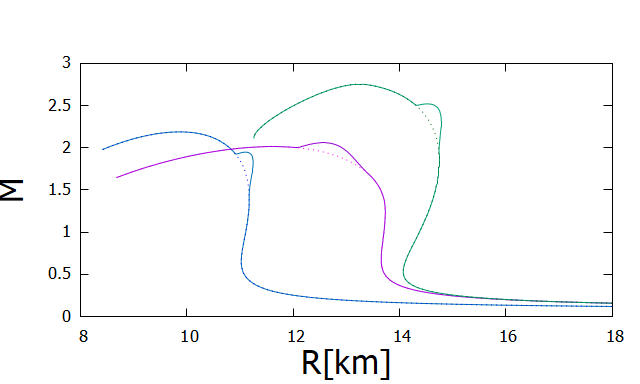
In Fig. 2, we show the mass-radius relation for three EOSs for the conformal attractor model Eq. (18) with $p=2.3$ (solid) and GR (dotted). The physical radius of a neutron star $R$ is defined in terms of the surface of the star $r_{*}$ by $R=e^{a({\varphi}(r_{*}))}r_{*}$. Among three EOSs, MS1 is the stiffest (large $p_{1}$) EOS and the radius of a $1.4M_{\odot}$ neutron star is large ($\sim 14.6{\rm km}$ in GR), while APR4 is a soft EOS and the radius of a $1.4M_{\odot}$ neutron star is small ($\sim 11.2{\rm km}$). In fact, a strong correlation between the pressure at around the nuclear saturation density $\rho_{\rm nuc}$ and the radius of $1.4M_{\odot}$ neutron stars has been found Lattimer:2000nx . H4 is in between the two EOSs. On the other hand, the maximum mass of a neutron star (in GR) is the largest for MS1 ($\sim 2.75M_{\odot}$), while the smallest for H4 ($\sim 2.01M_{\odot}$) but is still compatible with the most massive pulsar ($2.08\pm 0.07M_{\odot}$) measured by NANOGrav:2019jur ; Fonseca:2021wxt .

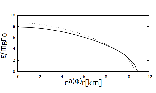
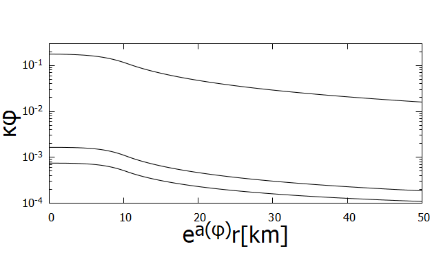
We also show the radial profile of the energy density $\epsilon$ in unit of $m_{B}n_{0}=1.66\times 10^{14}{\rm g/cm^{3}}$ for APR4 EOS in the left of Fig. 3 and the radial profile of the scalar field ${\varphi}$ in the right.

For each EOS, we compute the total gravitational (ADM) mass $M_{A}$ of the neutron star which is easily read off from the asymptotic behavior of $\mu(r)$ at infinity as $G_{*}M_{A}=\lim_{r\rightarrow\infty}\mu(r)$. Also, from the asymptotic behavior of ${\varphi}$, $\kappa{\varphi}\rightarrow\kappa{\varphi}_{0}+G_{*}M_{S}/r$, we compute the scalar charge $M_{S}$ of the neutron star. The effective scalar coupling $\alpha_{A}$ introduced in Damour:1992we ; Damour:1993hw is written in terms of $M_{A}$ and $M_{S}$ as (note again that our ${\varphi}$ is related to the scalar field ${\varphi}_{\rm DEF}$ in Damour:1992we ; Damour:1993hw via ${\varphi}_{\rm DEF}=\kappa{\varphi}/\sqrt{2}$)

$\displaystyle\alpha_{A}=\frac{\sqrt{2}}{\kappa}\frac{\partial\ln M_{A}}{\partial{\varphi}}=-\frac{M_{S}}{\sqrt{2}M_{A}}.$

(35)

We consider the following 6 NS-WD binaries: PSRs J0348+0432Antoniadis:2013pzd , J1738+03332012MNRAS.423.3328F , J1012+53072009MNRAS.400..805L ; 2020MNRAS.494.4031M ; 2020ApJ…896…85D , J1713+07472019MNRAS.482.3249Z , and J2222-01372017ApJ…844..128C ; Guo:2021bqa , J1909-37442020MNRAS.499.2276L .

For PSR J1012+5307, the limit on the scalar coupling $\alpha_{A}$ from the absence of the dipole radiation is recently improved in 2020ApJ…896…85D by the precise measurement of the distance by VLBI. Moreover, the mass of the neutron star is determined recently due to an estimate of the mass of the white dwarf companion using binary evolution models 2020MNRAS.494.4031M . For PSR J2222-0137, the limit on the scalar coupling is recently improved in Guo:2021bqa compared with 2017ApJ…844..128C by the improved analysis of VLBI data together with the extended timing data. For PSR 1713+0747, PSR J2222-0137 and PSR J1909-3744, the pulsar mass is determined from the Shapiro time-delays, while for others the pulsar mass is determined from the combination of the white dwarf mass determined from the optical spectrum and the mass ratio determined from the orbital velocity.

The measurements of the orbital decay of the binary systems are consistent with the orbital decay due to the emission of gravitational waves predicted by GR Peters:1964zz :

$\displaystyle\dot{P}_{b}^{GR}=-\frac{192\pi}{5}\frac{\left(1+{73}e^{2}/24+{37}e^{4}/96\right)}{(1-e^{2})^{7/2}}\left(\frac{2\pi}{P_{b}}\frac{G_{*}M_{c}}{c^{3}}\right)^{5/3}\frac{q}{(q+1)^{1/3}},$

(36)

where $e$ is the orbital eccentricity, $P_{b}$ is the orbital period, $M_{c}$ is the companion (white dwarf) mass and $q=M_{A}/M_{c}$ is the ratio of the pulsar mass to the companion mass. In scalar-tensor theory, scalar waves are also emitted and contribute the orbital decay. For the binary systems, the dominant contribution comes from dipolar waves Damour:1992we :

$\displaystyle\dot{P}_{b}^{D}=-2\pi\frac{\left(1+e^{2}/2\right)}{(1-e^{2})^{5/2}}\left(\frac{2\pi}{P_{b}}\frac{G_{*}M_{c}}{c^{3}}\right)\frac{q}{q+1}(\alpha_{A}-\alpha_{c})^{2},$

(37)

where $\alpha_{c}$ are the effective scalar coupling to white dwarf. Since the self-gravity of white dwarf is small, $\alpha_{c}$ is no different from its asymptotic value: $\alpha_{c}\simeq\sqrt{2}\alpha({\varphi}_{0})/\kappa\ll 1$. The measurements of $\dot{P}_{b}$ constrain the dipole contribution, hence $\alpha_{A}-\alpha_{c}\simeq\alpha_{A}$. The parameters of six NS-WD binaries and the $2\sigma$ limits on $\alpha_{A}$ are shown in Table 1.

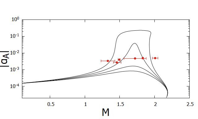
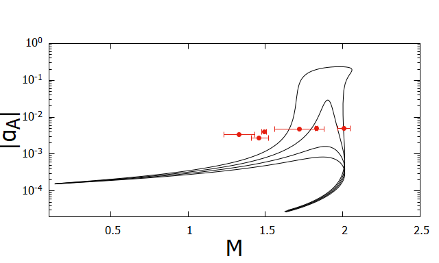
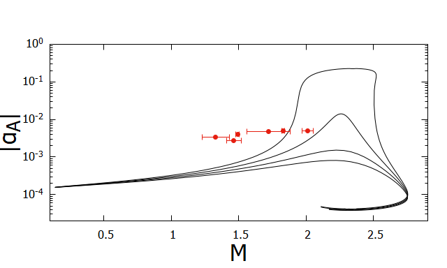
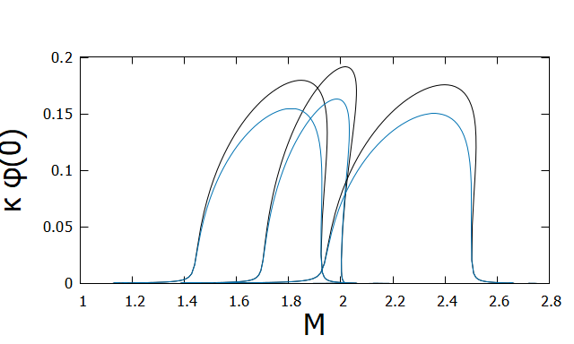
In Fig. 4, $\alpha_{A}$ as a function of the gravitational mass of the neutron stars for three EOSs together with the 2$\sigma$ limits on $\alpha_{A}$ from the pulsar-timings are shown. We find that spontaneous scalarization occurs if $p\gtrsim 2.2$ and $p$ is constrained as $p<2.3$ irrespective of EOSs. ⁹⁹9The weak dependence of the onset of the scalarization on the EOS was found in Harada:1997mr ; Novak:1998rk . However, more detailed constraints on $p$ depend on the EOS: $p$ is constrained to be $p<2.2$ for APR4 and H4, while $p=2.2$ is allowed for MS1. We may place a conservative limit on $p$ to be $p<2.3$. Although there exist small windows for the scalarization at $\sim 1.9M_{\odot}$ for H4 and at $\sim 2.3M_{\odot}$ for MS1 Shao:2017gwu , a “window at $\sim 1.7M_{\odot}$” Shao:2017gwu is now closed with the inclusion of PSR J1012+5307 and PSR J2222-0137.

So far, the effective scalar coupling is computed for the coupling function Eq. (18). However, most frequently studied gravity theory is the so-called DEF theory Damour:1993hw based on the quadratic coupling function :

$\displaystyle a({\varphi})=\frac{1}{2}\beta(\kappa{\varphi})^{2}.$

(38)

Eq. (18) can be expanded as $a({\varphi})=-\frac{1}{2}p(\kappa{\varphi})^{2}+{O}((k{\varphi})^{4})$ for $\kappa{\varphi}\ll 1$, hence $p$ corresponds to $-\beta$ in the quadratic model. Note that since ${\varphi}_{\rm DEF}$ in Damour:1993hw corresponds to ${\varphi}_{\rm DEF}=\kappa{\varphi}/\sqrt{2}$, $\beta_{\rm DEF}$ in $a({\varphi}_{\rm DEF})=\frac{1}{2}\beta_{\rm DEF}{\varphi}_{\rm DEF}^{2}$ corresponds to $\beta_{\rm DEF}=2\beta$.

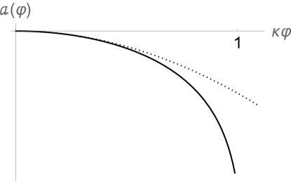
Although the coupling function $a({\varphi})$ in Eq. (18) is well approximated as $a({\varphi})=-\frac{1}{2}p(\kappa{\varphi})^{2}$ as long as $\kappa{\varphi}\ll 1$ (see Fig. 5), the scalar field may acquire a large value when the theory exhibits spontaneous scalarization and the scalar field can experience a wider portion of the coupling function.

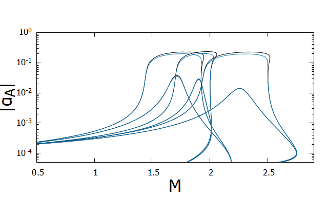
However, as shown in Fig. 6, even for $p=2.3$, the difference of $\alpha_{A}$ between the two coupling functions is very small. For $p=2.2$, two $\alpha_{A}$s almost coincide. In fact, as shown in Fig. 7, the maximum value of the scalar field (${\varphi}(0)$) is at most $\kappa{\varphi}(0)\lesssim 0.2$ even for $p=2.3$ and higher order terms in the Taylor expansion of $a({\varphi})$ is negligible. Similar results are obtained by Anderson:2019eay from the comparison of the quadratic model and MO model Mendes:2016fby .

This behavior can be understood from the stability analysis of neutron stars in scalar-tensor theories Harada:1997mr ; Harada:1998ge . Spontaneous scalarization is triggered by a tachyonic instability of the scalar field of a general relativistic star. From the linear stability analysis of neutron stars, the threshold value of the curvature of the coupling function is found to be insensitive to EOSs Harada:1997mr . In the linear analysis, only the quadratic term in $a({\varphi})$ is relevant and possible higher order terms are not important in the analysis. Moreover, using the catastrophe theory, it is shown that the onset of spontaneous scalarization in the quadratic coupling function corresponds to cusp catastrophe Harada:1998ge which is structurally stable, i.e. the theory is stable against adding higher order terms in the coupling function. Therefore, we expect that the structure of the theory near the onset of the scalarization is described by the quadratic coupling function universally.

Since pulsar data already disfavor $p\geq 2.3$, we thus conclude that as far as the observational constraints on spontaneous scalarization are concerned, it is sufficient to employ the quadratic function for the coupling function.

Finally we comment on the cosmological evolution of ${\varphi}$ which defines its asymptotic value ${\varphi}_{0}$.

As we have seen in 2.2, the conformal attractor model is cosmologically attracted toward the conformal symmetry $\omega\rightarrow-3/2$, in vast disagreement with the solar system experiments. Therefore, similar to the quadratic function with negative curvature, a severe fine-tuning of the initial conditions is required to satisfy the solar system constraints todaySampson:2014qqa .

One obvious and the simplest possibility to avoid this problem is to introduce a mass term for ${\varphi}$ (in the Einstein frame)Chen:2015zmx ; Ramazanoglu:2016kul ; dePireySaintAlby:2017lwc . Massive scalar-tensor theories with mass $m_{{\varphi}}$ of $10^{-28}{\rm eV}\lesssim m_{{\varphi}}\lesssim 10^{-10}{\rm eV}$ may both exhibit spontaneous scalarization (upper bound) and cosmological attraction toward GR in the matter-dominated era (lower bound). According to Ramazanoglu:2016kul , the effective scalar coupling of a neutron star is not different from that of a massless theory if $m_{{\varphi}}\lesssim 10^{-13}{\rm eV}$ but is much suppressed for $m_{{\varphi}}\gtrsim 10^{-12}{\rm eV}$.¹⁰¹⁰10 $m_{{\varphi}}\lesssim 10^{-17}{\rm eV}$ may be required for the success of the big-bang nucleosynthesis dePireySaintAlby:2017lwc . If this is the case, the structure of neutron stars would be almost the same as that of a massless theory.

References

- (1) P. G. Bergmann, Comments on the scalar tensor theory, Int. J. Theor. Phys. 1 (1968) 25.
- (2) K. Nordtvedt, Jr., PostNewtonian metric for a general class of scalar tensor gravitational theories and observational consequences, Astrophys. J. 161 (1970) 1059.
- (3) R. V. Wagoner, Scalar tensor theory and gravitational waves, Phys. Rev. D1 (1970) 3209.
- (4) C. Will, Theory and experiment in gravitational physics. Cambridge University Press, Cambridge, 2 ed., 2018.
- (5) K. Nordtvedt, Equivalence Principle for Massive Bodies. 2. Theory, Phys. Rev. 169 (1968) 1017.
- (6) F. Hofmann and J. Müller, Relativistic tests with lunar laser ranging, Class. Quant. Grav. 35 (2018) 035015.
- (7) B. M. Barker, General scalar-tensor theory of gravity with constant G., Astrophys. J. 219 (1978) 5.
- (8) T. Damour and G. Esposito-Farese, Tensor multiscalar theories of gravitation, Class. Quant. Grav. 9 (1992) 2093.
- (9) J.-M. Gerard, The Strong equivalence principle from gravitational gauge structure, Class. Quant. Grav. 24 (2007) 1867 [gr-qc/0607019].
- (10) R. Kallosh and A. Linde, Universality Class in Conformal Inflation, JCAP 07 (2013) 002 [1306.5220].
- (11) R. Kallosh and A. Linde, Multi-field Conformal Cosmological Attractors, JCAP 12 (2013) 006 [1309.2015].
- (12) I. Bars, S.-H. Chen, P. J. Steinhardt and N. Turok, Antigravity and the Big Crunch/Big Bang Transition, Phys. Lett. B 715 (2012) 278 [1112.2470].
- (13) I. Bars, P. Steinhardt and N. Turok, Local Conformal Symmetry in Physics and Cosmology, Phys. Rev. D 89 (2014) 043515 [1307.1848].
- (14) T. Damour and G. Esposito-Farese, Nonperturbative strong field effects in tensor - scalar theories of gravitation, Phys. Rev. Lett. 70 (1993) 2220.
- (15) T. Harada, Stability analysis of spherically symmetric star in scalar - tensor theories of gravity, Prog. Theor. Phys. 98 (1997) 359 [gr-qc/9706014].
- (16) J. Novak, Neutron star transition to strong scalar field state in tensor scalar gravity, Phys. Rev. D 58 (1998) 064019 [gr-qc/9806022].
- (17) T. Damour and G. Esposito-Farese, Gravitational wave versus binary - pulsar tests of strong field gravity, Phys. Rev. D 58 (1998) 042001 [gr-qc/9803031].
- (18) M. Shibata, K. Taniguchi, H. Okawa and A. Buonanno, Coalescence of binary neutron stars in a scalar-tensor theory of gravity, Phys. Rev. D 89 (2014) 084005 [1310.0627].
- (19) L. Shao, N. Sennett, A. Buonanno, M. Kramer and N. Wex, Constraining nonperturbative strong-field effects in scalar-tensor gravity by combining pulsar timing and laser-interferometer gravitational-wave detectors, Phys. Rev. X 7 (2017) 041025 [1704.07561].
- (20) N. Wex and M. Kramer, Gravity Tests with Radio Pulsars, Universe 6 (2020) 156.
- (21) D. Anderson, P. Freire and N. Yunes, Binary pulsar constraints on massless scalar–tensor theories using Bayesian statistics, Class. Quant. Grav. 36 (2019) 225009 [1901.00938].
- (22) R. F. P. Mendes and N. Ortiz, Highly compact neutron stars in scalar-tensor theories of gravity: Spontaneous scalarization versus gravitational collapse, Phys. Rev. D 93 (2016) 124035 [1604.04175].
- (23) B. Bertotti, L. Iess and P. Tortora, A test of general relativity using radio links with the Cassini spacecraft, Nature 425 (2003) 374.
- (24) T. Damour and K. Nordtvedt, Tensor - scalar cosmological models and their relaxation toward general relativity, Phys. Rev. D 48 (1993) 3436.
- (25) T. Chiba and M. Yamaguchi, Conformal-Frame (In)dependence of Cosmological Observations in Scalar-Tensor Theory, JCAP 10 (2013) 040 [1308.1142].
- (26) J. Antoniadis et al., A Massive Pulsar in a Compact Relativistic Binary, Science 340 (2013) 6131 [1304.6875].
- (27) J. S. Read, B. D. Lackey, B. J. Owen and J. L. Friedman, Constraints on a phenomenologically parameterized neutron-star equation of state, Phys. Rev. D 79 (2009) 124032 [0812.2163].
- (28) A. Akmal, V. R. Pandharipande and D. G. Ravenhall, The Equation of state of nucleon matter and neutron star structure, Phys. Rev. C 58 (1998) 1804 [nucl-th/9804027].
- (29) N. K. Glendenning and S. A. Moszkowski, Reconciliation of neutron star masses and binding of the lambda in hypernuclei, Phys. Rev. Lett. 67 (1991) 2414.
- (30) B. D. Lackey, M. Nayyar and B. J. Owen, Observational constraints on hyperons in neutron stars, Phys. Rev. D 73 (2006) 024021 [astro-ph/0507312].
- (31) H. Mueller and B. D. Serot, Relativistic mean field theory and the high density nuclear equation of state, Nucl. Phys. A 606 (1996) 508 [nucl-th/9603037].
- (32) F. Douchin and P. Haensel, A unified equation of state of dense matter and neutron star structure, Astron. Astrophys. 380 (2001) 151 [astro-ph/0111092].
- (33) J. M. Lattimer and M. Prakash, Neutron star structure and the equation of state, Astrophys. J. 550 (2001) 426 [astro-ph/0002232].
- (34) NANOGrav collaboration, Relativistic Shapiro delay measurements of an extremely massive millisecond pulsar, Nature Astron. 4 (2019) 72 [1904.06759].
- (35) E. Fonseca et al., Refined Mass and Geometric Measurements of the High-mass PSR J0740+6620, Astrophys. J. Lett. 915 (2021) L12 [2104.00880].
- (36) P. C. C. Freire, N. Wex, G. Esposito-Farèse, J. P. W. Verbiest, M. Bailes, B. A. Jacoby et al., The relativistic pulsar-white dwarf binary PSR J1738+0333 - II. The most stringent test of scalar-tensor gravity, MNRAS 423 (2012) 3328 [1205.1450].
- (37) K. Lazaridis, N. Wex, A. Jessner, M. Kramer, B. W. Stappers, G. H. Janssen et al., Generic tests of the existence of the gravitational dipole radiation and the variation of the gravitational constant, MNRAS 400 (2009) 805 [0908.0285].
- (38) D. Mata Sánchez, A. G. Istrate, M. H. van Kerkwijk, R. P. Breton and D. L. Kaplan, PSR J1012+5307: a millisecond pulsar with an extremely low-mass white dwarf companion, MNRAS 494 (2020) 4031 [2004.02901].
- (39) H. Ding, A. T. Deller, P. Freire, D. L. Kaplan, T. J. W. Lazio, R. Shannon et al., Very Long Baseline Astrometry of PSR J1012+5307 and its Implications on Alternative Theories of Gravity, ApJ 896 (2020) 85 [2004.14668].
- (40) W. W. Zhu et al., Tests of Gravitational Symmetries with Pulsar Binary J1713+0747, Mon. Not. Roy. Astron. Soc. 482 (2019) 3249 [1802.09206].
- (41) I. Cognard, P. C. C. Freire, L. Guillemot, G. Theureau, T. M. Tauris, N. Wex et al., A Massive-born Neutron Star with a Massive White Dwarf Companion, ApJ 844 (2017) 128 [1706.08060].
- (42) Y. J. Guo et al., PSR J2222–0137. I. Improved physical parameters for the system, Astron. Astrophys. 654 (2021) A16 [2107.09474].
- (43) K. Liu, L. Guillemot, A. G. Istrate, L. Shao, T. M. Tauris, N. Wex et al., A revisit of PSR J1909-3744 with 15-yr high-precision timing, MNRAS 499 (2020) 2276 [2009.12544].
- (44) P. C. Peters, Gravitational Radiation and the Motion of Two Point Masses, Phys. Rev. 136 (1964) B1224.
- (45) T. Harada, Neutron stars in scalar tensor theories of gravity and catastrophe theory, Phys. Rev. D 57 (1998) 4802 [gr-qc/9801049].
- (46) L. Sampson, N. Yunes, N. Cornish, M. Ponce, E. Barausse, A. Klein et al., Projected Constraints on Scalarization with Gravitational Waves from Neutron Star Binaries, Phys. Rev. D 90 (2014) 124091 [1407.7038].
- (47) P. Chen, T. Suyama and J. Yokoyama, Spontaneous scalarization: asymmetron as dark matter, Phys. Rev. D 92 (2015) 124016 [1508.01384].
- (48) F. M. Ramazanoğlu and F. Pretorius, Spontaneous Scalarization with Massive Fields, Phys. Rev. D 93 (2016) 064005 [1601.07475].
- (49) T. A. de Pirey Saint Alby and N. Yunes, Cosmological Evolution and Solar System Consistency of Massive Scalar-Tensor Gravity, Phys. Rev. D 96 (2017) 064040 [1703.06341].