Stability and Hopf bifurcation analysis of a two state delay differential equation modeling the human respiratory system

Nirjal Sapkota Electronic address: nxs167030@utdallas.edu; Corresponding author Department of Mathematical Sciences,
The University of Texas at Dallas
Richardson, TX, 75080, USA Janos Turi Electronic address: turi@utdallas.edu Department of Mathematical Sciences,
The University of Texas at Dallas
Richardson, TX, 75080, USA

Abstract

We study the two state model which describes the balance equation for carbon dioxide and oxygen. These are nonlinear parameter dependent and because of the transport delay in the respiratory control system, they are modeled with delay differential equation. So, the dynamics of a two state one delay model are investigated. By choosing the delay as a parameter, the stability and Hopf bifurcation conditions are obtained. We notice that as the delay passes through its critical value, the positive equilibrium loses its stability and Hopf bifurcation occurs. The stable region of the system with delay against the other parameters and bifurcation diagrams are also plotted. The three dimensional stability chart of the two state model is constructed. We find that the delay parameter has effect on the stability but not on the equilibrium state. The explicit derivation of the direction of Hopf bifurcation and the stability of the bifurcation periodic solutions are determined with the help of normal form theory and center manifold theorem to delay differential equations. Finally, some numerical example and simulations are carried out to confirm the analytical findings. The numerical simulations verify the theoretical results.

1 Introduction

In human respiratory system, the goal is to exchange the unwanted byproduct such as carbon dioxide for oxygen. The carbon dioxide is exchanged for oxygen by passive diffusion. Alveoli is the tiny air sacs in the lungs where the exchange of oxygen and carbon dioxide takes place. The respiratory control system changes the rate of ventilation in response to the levels of oxygen and carbon dioxide in the body. The time delay is due to the physical distance where carbon dioxide and oxygen level information is transported to the sensory control system before the ventilatory response can be adapted.

Understanding the human respiratory system is important for many medical conditions. The human respiratory and its control mechanics have been studied for more than hundred years. This system has important medical implications some of which are listed below [6, 28, 23, 15]. {outline} \1 Periodic Breathing: Periodic Breathing is define as three or more episodes of central apnea lasting at least 3 seconds, separated by no more than 20 seconds of normal breathing. . \1 Sleep Apnea: Sleep Apnea is a disorder in which breathing repeatedly stops and stars again. It is classified in two ways. \2 Central Sleep Apnea is a disorder which is characterized by a lack of drive to breathe. \2 Obstructive Sleep Apnea is a disorder which is characterized by episodes of partial or complete physical obstruction of the airflow. \1 Cheyne-Stokes Respiration: Cheyne-Stokes Respiration is a disorder which is characterized by gradual increase in breathing followed by decrease or absence of breathing.

These disorders have been associated with a number of medical conditions such as hypertension, heart failures, diabetes and others [27, 21, 1].

1.1 Components of the Model

The carbon dioxide and oxygen levels are monitored at two respiratory centers in the body. These are called central and peripheral chemoreceptors.

1.1.1 Central chemoreceptors

Central chemoreceptors are located at the ventral surface of the medulla in the brain. These respond to the changes in the partial pressure of carbon dioxide in the brain.

1.1.2 Peripheral chemoreceptors

Peripheral chemoreceptors are located in the carotid bodies at the junction of the common carotid arteries and also at the aortic bodies. These respond to the changes in the partial pressure of both carbon dioxide and oxygen in arterial blood.

Since these respiratory centers are located at a distance from the lungs where the levels of the carbon dioxide and oxygen are regulated, there will be some delay (two transport delays) in the process. This regulation is modeled with the ventilation function.

1.1.3 Ventilation function

We assume some conditions for the ventilation functions $V(x,y)$ to be biologically realistic model.

•

$V(x,y)\geq 0$ and $V(0,0)=0$
•

$V(x,y)$ is differentiable
•

$V(x,y)$ is an increasing function in both $x$ and $y$
•

$\frac{\partial V(x,y)}{\partial x}>0$ and $\frac{\partial V(x,y)}{\partial y}>0$

1.2 Model equation

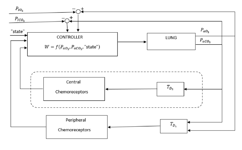
Although a five-state model involving three compartments and two control loops with multiple delays is investigated in [23], here we will study a two state model with one time delay discussed in [12] and [24]. A block diagram of the respiratory system is shown in Figure 1. The controller adjusts to inputs from the state (i.e., sleep, wakefulness) and the chemoreceptors which respond to the change in carbon dioxide and oxygen concentration.

Refer to caption — Figure 1: Block diagram of respiratory control system

We consider the following two state model for studying stability and bifurcation of a human respiratory system.

	$\displaystyle\frac{\mathrm{d}\tilde{x}}{\mathrm{d}t}$	$\displaystyle=p-\alpha\,W(\tilde{x}(t-\tau),\tilde{y}(t-\tau))(\tilde{x}(t)-x_{I})$		(1)
	$\displaystyle\frac{\mathrm{d}\tilde{y}}{\mathrm{d}t}$	$\displaystyle=-\sigma+\beta\,W(\tilde{x}(t-\tau),\tilde{y}(t-\tau))(y_{I}-\tilde{y}(t))$		(1)

where

•

$\tilde{x}(\cdot)$ , $\tilde{y}(\cdot)$ represent the arterial carbon dioxide and oxygen concentration
•

$W(\cdot,\cdot)$ is the ventilation function which represents the volume of gas moved by the respiratory system
•

$\tau$ is the transport delay ( $\tau>0$ and $\tau=T_{D_{1}}$ in Figure 1)
•

$x_{I}$ , $y_{I}$ are inspired carbon dioxide and oxygen concentration
•

$p$ is the carbon dioxide production rate
•

$\sigma$ is the oxygen consumption rate
•

$\alpha$ , $\beta$ are positive constants associated with the diffusibility of carbon dioxide and oxygen respectively

For studying the stability analysis with a more convenient system, we convert the system (1) using

	$\displaystyle x(t)$	$\displaystyle=a(\tilde{x}(t)-x_{I})$		(2)
	$\displaystyle y(t)$	$\displaystyle=b(y_{I}-\tilde{y}(t))$		(2)

Solving for $\tilde{x}(t-\tau)$ and $\tilde{y}(t-\tau)$ , we get,

	$\displaystyle\tilde{x}(t-\tau)$	$\displaystyle=x_{I}+\frac{1}{a}x(t-\tau)$		(3)
	$\displaystyle\tilde{y}(t-\tau)$	$\displaystyle=y_{I}-\frac{1}{b}y(t-\tau)$		(3)

Using Equation (3) in Equation (1), we obtain

	$\displaystyle\frac{\mathrm{d}x}{\mathrm{d}t}$	$\displaystyle=a\frac{\mathrm{d}\tilde{x}}{\mathrm{d}t}=ap-a\alpha W\left(x_{I}+\frac{1}{a}x(t-\tau),y_{I}-\frac{1}{b}y(t-\tau)\right)\frac{x(t)}{a}$		(4)
	$\displaystyle\frac{\mathrm{d}y}{\mathrm{d}t}$	$\displaystyle=-b\frac{\mathrm{d}\tilde{y}}{\mathrm{d}t}=b\sigma-b\beta W\left(x_{I}+\frac{1}{a}x(t-\tau),y_{I}-\frac{1}{b}y(t-\tau)\right)\frac{y(t)}{a}$		(4)

Setting $a=1/p$ and $b=1/\sigma$ , we obtain the equations

	$\displaystyle\frac{\mathrm{d}x}{\mathrm{d}t}$	$\displaystyle=1-\alpha\,V(x(t-\tau),y(t-\tau))\,x(t)$		(5)
	$\displaystyle\frac{\mathrm{d}y}{\mathrm{d}t}$	$\displaystyle=1-\beta\,V(x(t-\tau),y(t-\tau))\,y(t)$		(5)

where the ventilation function is given by

V(x(t-\tau),y(t-\tau))=W(\tilde{x}(t-\tau),\tilde{y}(t-\tau))

(6)

We will study the system (5) with

V(x(t-\tau),y(t-\tau))=0.14\,e^{-0.05(100-y(t-\tau))}\,x(t-\tau)

(7)

The state variables are concentrations in our model.

2 Stability and Hopf Bifurcation

In recent years, a lot of delay differential equations modeling various chemical, biological, ecological systems have been studied [8, 14, 16, 43, 36, 50, 5, 39]. With the outbreak of COVID-19 pandemic, many mathematical models using delay differential equations have been proposed [35, 38, 40, 37, 13, 19, 33].

Li and Zhang [30], Bılazeroğlu [9], studied the dynamic analysis and Hopf bifurcation of a Lengyel-Epstein system with two delays. Li [32] studied a class of delay differential equations with two delays. Kumar et al [25] proposed a multiple delayed innovation diffusion model with Holling II functional response. Delayed predator-prey system have been investigated by many researchers ([42, 51, 2, 41, 22, 52, 47, 44, 11, 10, 45, 53]). Ghosh et al [17] studied the rumor spread mechanism and the influential factors using epidemic like model. Several researchers have analyzed the Uçar prototype system [46, 7, 29, 31]. Wei [48] discussed the dynamics of a scalar delay differential equation. Gilsinn [18] estimates the bifurcation parameter of delay differential equation with application to machine tool chatter. There has been a focus on studying stability and Hopf bifurcation by choosing the delay as a parameter of the system with the linear stability methods.

The complex system modeling the human respiratory control system have been studied for several decades. Mackey and Glass [34], Khoo et al [23], Batzel et al [4, 3] have investigated stability analysis.

2.1 Equilibrium point

Lemma 2.1.

There is a unique positive equilibrium point $E_{*}(x_{*},y_{*})$ of system (5).

Proof.

The equilibrium point $E_{*}(x_{*},y_{*})$ is obtained by solving

	$\displaystyle 1-\alpha\,0.14\,e^{-0.05(100-y_{})}x_{}^{2}$	$\displaystyle=0$		(8)
	$\displaystyle 1-\beta\,0.14\,e^{-0.05(100-y_{})}y_{}$	$\displaystyle=0$		(8)

We also notice that

x_{*}\neq 0,y_{*}\neq 0,\text{ and }x_{*}=\frac{\beta}{\alpha}y_{*}

Then, rewriting as exact fractions and solving the equation

1-\alpha\left(\frac{14}{100}\right)\,e^{-\frac{5}{100}(100-y_{*})}\frac{\beta^{2}y_{*}^{2}}{\alpha^{2}}=0

(9)

we get,

y_{*}=40\,W\left(\frac{e^{5/2}\sqrt{\frac{\alpha}{\beta^{2}}}}{4\sqrt{14}}\right)

(10)

and

x_{*}=40\,\left(\frac{\beta}{\alpha}\right)W\left(\frac{e^{5/2}\sqrt{\frac{\alpha}{\beta^{2}}}}{4\sqrt{14}}\right)

(11)

where $W$ represents the Lambert $W$ -function.
Since $V(0,0)=0$ and

V\left(\frac{\beta y_{*}}{\alpha},y^{*}\right)=\left(\frac{14}{100}\right)\,e^{-\frac{5}{100}(100-y_{*})}\frac{\beta y_{*}}{\alpha}

is increasing in $y_{*},$ there is a unique positive solution $y_{*}$ .
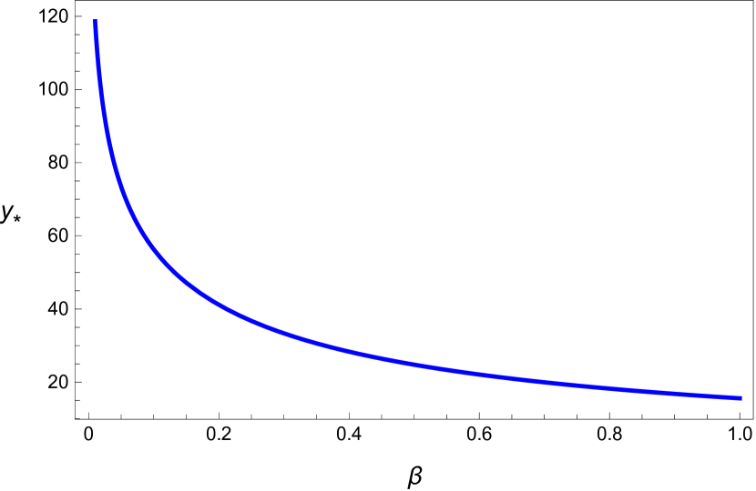
For the default values of $\alpha=0.5$ and $\beta=0.8$ , we get $(x_{*},y_{*})\approx(29.1842,18.2401).$

∎

We plot the Equations (11) and (10) as a function of $\alpha$ and $\beta$ in Figure 2 and 3.

2.2 Stability of the Equilibrium point

Let $u(t)=x(t)-x_{*},\,v(t)=y(t)-y_{*}.$ Then, the linearized system of (5) is given as follows:

	$\displaystyle\frac{\mathrm{d}u(t)}{\mathrm{d}t}$	$\displaystyle=-\alpha V(x_{},y_{})u(t)-\alpha x_{}V_{x}(x_{},y_{})u(t-\tau)-\alpha x_{}V_{y}(x_{},y_{})v(t-\tau)$		(12)
	$\displaystyle\frac{\mathrm{d}v(t)}{\mathrm{d}t}$	$\displaystyle=-\beta V(x_{},y_{})v(t)-\beta y_{}V_{x}(x_{},y_{})v(t-\tau)-\beta y_{}V_{y}(x_{},y_{})v(t-\tau)$		(12)

This could be written in the form as

\frac{\mathrm{d}}{\mathrm{d}t}\begin{pmatrix}u(t)\\ v(t)\end{pmatrix}+A_{1}\begin{pmatrix}u(t)\\ v(t)\end{pmatrix}+B_{1}\begin{pmatrix}u(t-\tau)\\ v(t-\tau)\end{pmatrix}=\begin{pmatrix}0\\ 0\end{pmatrix}

(13)

where

A_{1}=\begin{pmatrix}\alpha V(x_{*},y_{*})&0\\ 0&\beta V(x_{*},y_{*})\end{pmatrix}=\left(\begin{array}[]{cc}\frac{7}{50}\alpha x_{*}e^{\frac{1}{20}\left(y_{*}-100\right)}&0\\ 0&\frac{7}{50}\beta x_{*}e^{\frac{1}{20}\left(y_{*}-100\right)}\\ \end{array}\right)

and

B_{1}=\begin{pmatrix}\alpha x_{*}V_{x}(x_{*},y_{*})&\alpha x_{*}V_{y}(x_{*},y_{*})\\ \beta y_{*}V_{x}(x_{*},y_{*})&\beta y_{*}V_{y}(x_{*},y_{*})\end{pmatrix}=\left(\begin{array}[]{cc}\frac{7}{50}\alpha x_{*}e^{\frac{1}{20}\left(y_{*}-100\right)}&\frac{7\alpha x_{*}^{2}e^{\frac{1}{20}\left(y_{*}-100\right)}}{1000}\\ \frac{7}{50}\beta e^{\frac{1}{20}\left(y_{*}-100\right)}y_{*}&\frac{7\beta x_{*}e^{\frac{1}{20}\left(y_{*}-100\right)}y_{*}}{1000}\\ \end{array}\right)

The associated characteristic equation of the linear system (13) is

\Delta(\lambda,\tau)=\det(\lambda I+A_{1}+B_{1}e^{-\tau\lambda})=0

(14)

That is,

\lambda^{2}+\frac{7\lambda x_{*}e^{-\lambda\tau+\frac{y_{*}}{20}-5}\left(20(\alpha+\beta)e^{\lambda\tau}+20\alpha+\beta y_{*}\right)}{1000}+\frac{49\alpha\beta x_{*}^{2}e^{-\lambda\tau+\frac{y_{*}}{10}-10}\left(20e^{\lambda\tau}+y_{*}+20\right)}{50000}=0

(15)

This could be also written as

\Delta(\lambda,\tau)=\lambda^{2}+\left(A+Be^{-\lambda\tau}\right)\lambda+\left(C+De^{-\lambda\tau}\right)=0

(16)

where

$\displaystyle A$	$\displaystyle=\frac{7}{50}\alpha x_{}e^{\frac{y_{}}{20}-5}+\frac{7}{50}\beta x_{}e^{\frac{y_{}}{20}-5}$	(17)
$\displaystyle B$	$\displaystyle=\frac{7}{50}\alpha x_{}e^{\frac{y_{}}{20}-5}+\frac{7\beta x_{}e^{\frac{y_{}}{20}-5}y_{*}}{1000}$
$\displaystyle C$	$\displaystyle=\frac{49\alpha\beta x_{}^{2}e^{\frac{y_{}}{10}-10}}{2500}$
$\displaystyle D$	$\displaystyle=\frac{49\alpha\beta x_{}^{2}e^{\frac{y_{}}{10}-10}}{2500}+\frac{49\alpha\beta x_{}^{2}e^{\frac{y_{}}{10}-10}y_{*}}{50000}$

•

For $\tau=0$

The characteristic equation (15) simplifies to

\lambda^{2}+\frac{7\lambda x_{*}e^{\frac{y_{*}}{20}-5}\left(40\alpha+\beta\left(y_{*}+20\right)\right)}{1000}+\frac{49\alpha\beta x_{*}^{2}e^{\frac{y_{*}}{10}-10}\left(y_{*}+40\right)}{50000}=0

(18)

The coefficients in this equation are postivie, and therefore the roots have negative real parts.

•

For $\tau>0$

The change in stability of eigenvalue $\lambda$ can occur if $\text{Re}(\lambda)=0.$ Let $\lambda=i\omega$ and characteristic equation (16) takes the form

-\omega^{2}+i\omega\left(A+Be^{-i\tau\omega}\right)+\left(C+De^{-i\tau\omega}\right)=0

(19)

Solving for the real and imaginary parts of both sides, we get

	$\displaystyle C-\omega^{2}$	$\displaystyle=-B\omega\sin(\tau\omega)-D\cos(\tau\omega)$		(20)
	$\displaystyle A\omega$	$\displaystyle=D\sin(\tau\omega)-B\omega\cos(\tau\omega)$		(20)

Squaring and adding (20), we get the relation

f(\omega)=-\omega^{4}+\left(-A^{2}+B^{2}+2C\right)\omega^{2}+\left(-C^{2}+D^{2}\right)=0

(21)

Let

M=-A^{2}+B^{2}+2C=\frac{49\beta x_{*}^{2}e^{\frac{y_{*}}{10}-10}\left(-400\beta+40\alpha y_{*}+\beta y_{*}^{2}\right)}{1000000}

(22)

Then $M$ is positive if $40\alpha y_{*}+\beta y_{*}^{2}>400\beta$

and let

N=-C^{2}+D^{2}=\frac{2401\alpha^{2}\beta^{2}x_{*}^{4}e^{\frac{y_{*}}{5}-20}y_{*}\left(y_{*}+40\right)}{2500000000}>0

(23)

Assuming that $Y=\omega^{2}$ , we can write (21) as

\Phi(Y)=-Y^{2}+MY+N=0

(24)

This means that the Equation (24) has one positive root. Solving for $\tau$ from (20), we have the critical curves given by

\tau_{*}(n)=\\ \frac{2000\sqrt{2}e^{5}\pi n}{7\sqrt{\sqrt{N_{3}}+N_{4}}}\\ \pm\frac{1000i\sqrt{2}e^{5}\log\left(\frac{e^{-\frac{y_{*}}{20}}\left(\beta N_{2}x_{*}^{2}e^{\frac{y_{*}}{10}}\left(40\alpha+\beta N_{1}\right)-20i\sqrt{2}\sqrt{\sqrt{N_{3}}+N_{4}}x_{*}e^{\frac{y_{*}}{20}}(\alpha+\beta)+\sqrt{N_{3}}\right)}{x_{*}\left(40\alpha\beta N_{1}x_{*}e^{\frac{y_{*}}{20}}+i\sqrt{2}\sqrt{\sqrt{N_{3}}+N_{4}}\left(20\alpha+\beta y_{*}\right)\right)}\right)}{7\sqrt{\sqrt{N_{3}}+N_{4}}}\\ (n=0,\pm 1,\pm 2,...)

(25)

where

$\displaystyle N_{1}$	$\displaystyle=(y_{*}+20)$	(26)
$\displaystyle N_{2}$	$\displaystyle=(y_{*}-20)$
$\displaystyle N_{3}$	$\displaystyle=\beta^{2}x_{}^{4}e^{\frac{y_{}}{5}}\left(y_{}+20\right)\left(3200\alpha^{2}y_{}+80\alpha\beta\left(y_{}-20\right)y_{}+\beta^{2}\left(y_{}-20\right){}^{2}\left(y_{}+20\right)\right)$
$\displaystyle N_{4}$	$\displaystyle=\beta x_{}^{2}e^{\frac{y_{}}{10}}\left(40\alpha y_{}+\beta\left(y_{}^{2}-400\right)\right)$

Consequently, we can count that the stability region are restricted between the set of two curves

\tau_{1}(n)=\\ \frac{2000\sqrt{2}e^{5}\pi n}{7\sqrt{\sqrt{N_{3}}+N_{4}}}\\ +\frac{1000i\sqrt{2}e^{5}\log\left(\frac{e^{-\frac{y_{*}}{20}}\left(\beta N_{2}x_{*}^{2}e^{\frac{y_{*}}{10}}\left(40\alpha+\beta N_{1}\right)-20i\sqrt{2}\sqrt{\sqrt{N_{3}}+N_{4}}x_{*}e^{\frac{y_{*}}{20}}(\alpha+\beta)+\sqrt{N_{3}}\right)}{x_{*}\left(40\alpha\beta N_{1}x_{*}e^{\frac{y_{*}}{20}}+i\sqrt{2}\sqrt{\sqrt{N_{3}}+N_{4}}\left(20\alpha+\beta y_{*}\right)\right)}\right)}{7\sqrt{\sqrt{N_{3}}+N_{4}}}\\ (n=0,1,2,...)

(27)

\tau_{2}(n)=\\ \frac{2000\sqrt{2}e^{5}\pi n}{7\sqrt{\sqrt{N_{3}}+N_{4}}}\\ -\frac{1000i\sqrt{2}e^{5}\log\left(\frac{e^{-\frac{y_{*}}{20}}\left(\beta N_{2}x_{*}^{2}e^{\frac{y_{*}}{10}}\left(40\alpha+\beta N_{1}\right)-20i\sqrt{2}\sqrt{\sqrt{N_{3}}+N_{4}}x_{*}e^{\frac{y_{*}}{20}}(\alpha+\beta)+\sqrt{N_{3}}\right)}{x_{*}\left(40\alpha\beta N_{1}x_{*}e^{\frac{y_{*}}{20}}+i\sqrt{2}\sqrt{\sqrt{N_{3}}+N_{4}}\left(20\alpha+\beta y_{*}\right)\right)}\right)}{7\sqrt{\sqrt{N_{3}}+N_{4}}}\\ (n=1,2,...)

(28)

Notice that Equation (27) starts with $n=0,1,2,...$ and Equation (28) starts with $n=1,2,...$ for the pair of curves to have positive values of $\tau.$ If $\mathrm{Re}\left(d\lambda/d\tau\right)$ have different sign on any two consecutive critical curves, then the stability region is confined between these two curves in the $(\tau,\alpha,\beta)$ parameter space [26].

Now we look to verify the transversality condition:

\text{Re}\left(\frac{\mathrm{d}\lambda}{\mathrm{d}\tau}\right)>0

(29)

at $\tau=\tau_{*}$ with $n=0.$

Differentiating characteristic equation (16) with respect to $\tau$ , we get

2\lambda\frac{\mathrm{d}\lambda}{\mathrm{d}\tau}+\left(A+Be^{-\lambda\tau}\right)\frac{\mathrm{d}\lambda}{\mathrm{d}\tau}+Be^{-\lambda\tau}\lambda\left(-\lambda-\tau\frac{\mathrm{d}\lambda}{\mathrm{d}\tau}\right)+De^{-\lambda\tau}\left(-\lambda-\tau\frac{\mathrm{d}\lambda}{\mathrm{d}\tau}\right)=0

(30)

Solving for $\left[\mathrm{d}\lambda/\mathrm{d}\tau\right]^{-1},$ we get

	$\displaystyle\left[\frac{\mathrm{d}\lambda}{\mathrm{d}\tau}\right]^{-1}$	$\displaystyle=\frac{(A+2\lambda)e^{\lambda\tau}}{\lambda(B\lambda+D)}-\frac{B\lambda\tau-B+D\tau}{\lambda(B\lambda+D)}$		(31)
		$\displaystyle=-\frac{AD-BC+B\lambda^{2}+2D\lambda}{\lambda\left(A\lambda+C+\lambda^{2}\right)(B\lambda+D)}-\frac{\tau}{\lambda}$		(31)

On critical curves i.e with $\tau=\tau_{*}$ and $\lambda=i\omega$ , and solving for the real part, we have

$\displaystyle\text{Re}\left(\left[\frac{\mathrm{d}\lambda}{\mathrm{d}\tau}\right]^{-1}\right)$	$\displaystyle=\frac{A^{2}-2C+2\omega^{2}}{A^{2}\omega^{2}+\left(C-\omega^{2}\right)^{2}}-\frac{B^{2}}{B^{2}\omega^{2}+D^{2}}$	(32)
	$\displaystyle=\frac{A^{2}-2C+2\omega^{2}}{B^{2}\omega^{2}+D^{2}}-\frac{B^{2}}{B^{2}\omega^{2}+D^{2}}$
	$\displaystyle=\frac{A^{2}-B^{2}-2C+2\omega^{2}}{B^{2}\omega^{2}+D^{2}}$
	$\displaystyle=\frac{-C^{2}+D^{2}+\omega^{4}}{\omega^{2}\left(B^{2}\omega^{2}+D^{2}\right)}$
	$\displaystyle=\frac{N+\omega^{4}}{\omega^{2}\left(B^{2}\omega^{2}+D^{2}\right)}>0,\quad\textrm{since }N>0$

Since $\mathrm{Re}\left(d\lambda/d\tau\right)>0$ for all the critical curves (27) and (28), the corresponding slopes have positive values on all the stability determining critical curves. Thus, there are no eigenvalues with negative real part across the critical curves. Further, we know that for $\tau=0$ the equilibrium points $(x_{*},y_{*})$ are stable. Therefore, there can be only one stable region in the $(\tau,\alpha)$ or $(\tau,\beta)$ plane enclosed between the line $\tau=0$ and the curve $\tau_{1}(0).$

The critical curves for various $n$ as a function of $\alpha$ and $\beta$ are shown in Figures 4 and 5.

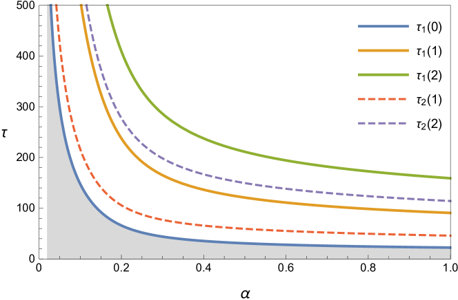
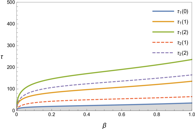
The critical surfaces in the parameter space $(\alpha,\beta,\tau)$ that encompass the stable region is shown in Figure 6.

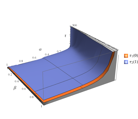
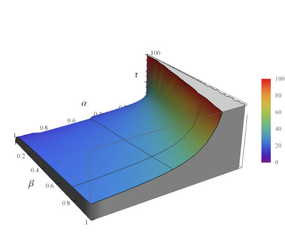
The 3 dimensional stability chart of the two state model of a human respiratory system in the parameter space $(\alpha,\beta,\tau)$ is shown in Figure 7.

For a more general case, the following theorem was proved in [12].

Theorem 2.2.

Let $V_{*}=V(x_{*},y_{*}),$ $V_{x*}=V_{x}(x_{*},y_{*})$ and $V_{y*}=V_{y}(x_{*},y_{*}).$

1.

If $V_{*}\geq x_{*}V_{x*}+y_{*}V_{y*},$ then the equilibrium $(x_{*},y_{*})$ is asymptotically stable for all delay $\tau\geq 0.$
2.

If $V_{*}<x_{*}V_{x*}+y_{*}V_{y*},$ then there exists $\tau_{*}>0$ such that the equilibrium $(x_{*},y_{*})$ is asymptotically stable if $0\leq\tau<\tau_{*}$ and unstable if $\tau>\tau_{*}.$

Therefore, from the above discussions, the following results can be directly deduced for our case.

Let $\tau_{*}$ be defined by (25). Then,

(i)

The positive equilibrium $E_{*}(x_{*},y_{*})$ of system (5) is asymptotically stable for $0\leq\tau<\tau_{*}$
(ii)

The positive equilibrium $E_{*}(x_{*},y_{*})$ of system (5) is unstable for $\tau>\tau_{*}$
(iii)

System (5) undergoes Hopf bifurcation at the positive equilibrium $E_{*}(x_{*},y_{*})$ for $\tau=\tau_{*}$

2.3 Critical Delay and Bifurcation

If we consider $\tau$ as a parameter, then as $\tau$ passes through its critical value $\tau_{*}$ , the positive equilibrium $E_{*}(x_{*},y_{*})$ loses its stability. The maximum value of the real part of the characteristic equation is computed for several values of $\tau.$ This is shown in figure 8. For the default values of $\alpha=0.5$ , $\beta=0.8$ , the equilibrium is $E_{*}(x_{*},y_{*})\approx(29.1842,18.2401)$ and the critical delay is $\tau_{*}\approx 30.8017.$

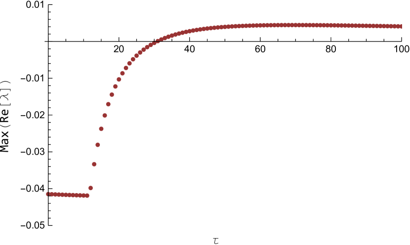
Table 1 lists the largest real part of the characteristic root computed for several values of $\tau$ near the critical delay with $\alpha=0.5$ and $\beta=0.8.$

Table 1: The largest real part of the eigenvalues with

\alpha=0.5

and

\beta=0.8

$\tau$	Max(Re[ $\lambda$ ])
25	-0.00386067
26	-0.0029966
27	-0.00222993
28	-0.00154774
29	-0.000939186
30	-0.000395051
31	0.0000925033
32	0.000530187
33	0.000923769
34	0.00127823
35	0.00159789

Figure 9 shows the maximum value of the real part of the characteristic equation for varying the parameters $\alpha$ and $\beta.$

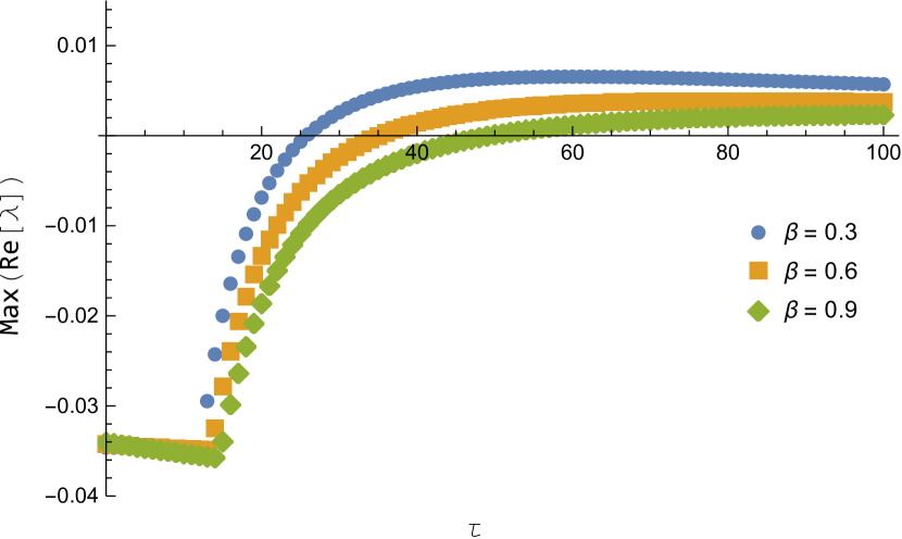
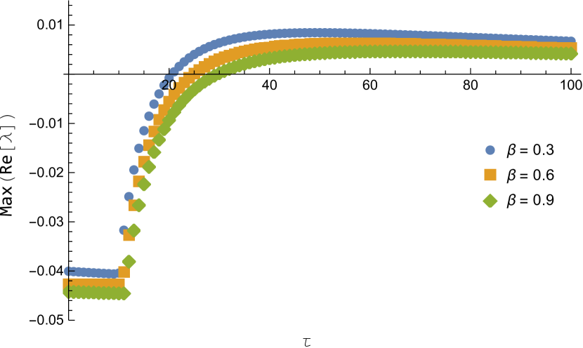
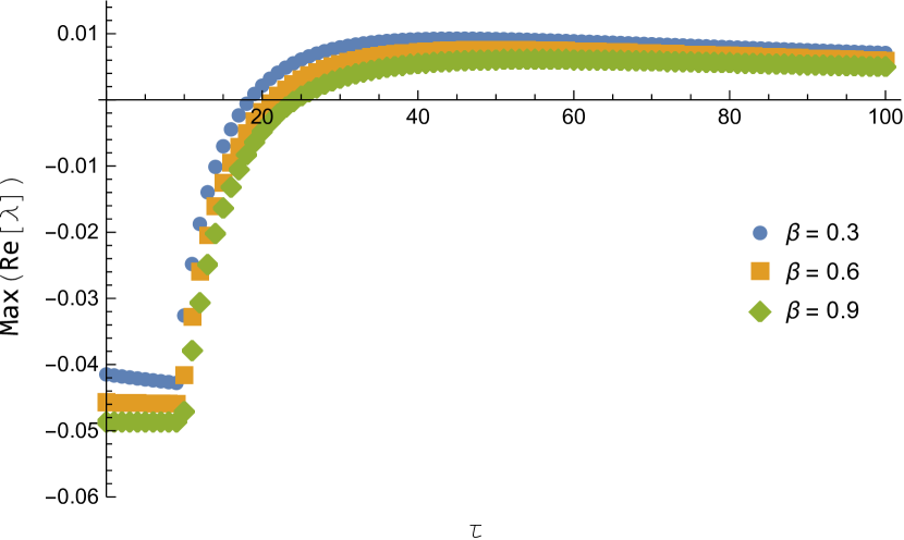
The following tables list out the largest part of the eigenvalues with various combination of $\alpha$ and $\beta$ near the critical delay.

Table 2: The largest real part of the eigenvalues with

\alpha=0.3

$\beta$	$\tau$	Max(Re[ $\lambda$ ])	$\beta$	$\tau$	Max(Re[ $\lambda$ ])	$\beta$	$\tau$	Max(Re[ $\lambda$ ])
0.3	20	-0.00686887	0.6	30	-0.00237351	0.9	45	-0.00076911
0.3	21	-0.00526380	0.6	31	-0.00181421	0.9	46	-0.00057352
0.3	22	-0.00387139	0.6	32	-0.00130903	0.9	47	-0.00039104
0.3	23	-0.00265816	0.6	33	-0.00085181	0.9	48	-0.00022063
0.3	24	-0.00159690	0.6	34	-0.00043725	0.9	49	-0.00006136
0.3	25	-0.00066533	0.6	35	-0.00006074	0.9	50	0.00008762
0.3	26	0.00015497	0.6	36	0.00028174	0.9	51	0.00022707
0.3	27	0.00087928	0.6	37	0.00059370	0.9	52	0.00035769
0.3	28	0.00152043	0.6	38	0.00087822	0.9	53	0.00048012
0.3	29	0.00208920	0.6	39	0.00113802	0.9	54	0.00059495
0.3	30	0.00259473	0.6	40	0.00137550	0.9	55	0.00070271

Table 3: The largest real part of the eigenvalues with

\alpha=0.6

$\beta$	$\tau$	Max(Re[ $\lambda$ ])	$\beta$	$\tau$	Max(Re[ $\lambda$ ])	$\beta$	$\tau$	Max(Re[ $\lambda$ ])
0.3	15	-0.01148690	0.6	20	-0.00560191	0.9	25	-0.00312474
0.3	16	-0.00853185	0.6	21	-0.00412443	0.9	26	-0.00229615
0.3	17	-0.00607124	0.6	22	-0.00284708	0.9	27	-0.00156234
0.3	18	-0.00400648	0.6	23	-0.00173803	0.9	28	-0.00091068
0.3	19	-0.00226226	0.6	24	-0.00077144	0.9	29	-0.00033055
0.3	20	-0.00078019	0.6	25	0.00007382	0.9	30	0.00018705
0.3	21	0.00048556	0.6	26	0.00081518	0.9	31	0.00064978
0.3	22	0.00157136	0.6	27	0.00146711	0.9	32	0.00106420
0.3	23	0.00250636	0.6	28	0.00204171	0.9	33	0.00143594
0.3	24	0.00331419	0.6	29	0.00254916	0.9	34	0.00176985
0.3	25	0.00401410	0.6	30	0.00299806	0.9	35	0.00207014

Table 4: The largest real part of the eigenvalues with

\alpha=0.9

$\beta$	$\tau$	Max(Re[ $\lambda$ ])	$\beta$	$\tau$	Max(Re[ $\lambda$ ])	$\beta$	$\tau$	Max(Re[ $\lambda$ ])
0.3	13	-0.01396730	0.6	16	-0.00957134	0.9	20	-0.00478992
0.3	14	-0.01012840	0.6	17	-0.00709898	0.9	21	-0.00339803
0.3	15	-0.00701248	0.6	18	-0.00502401	0.9	22	-0.00219773
0.3	16	-0.00445748	0.6	19	-0.00327084	0.9	23	-0.00115831
0.3	17	-0.00234397	0.6	20	-0.00178089	0.9	24	-0.00025488
0.3	18	-0.00058240	0.6	21	-0.00050815	0.9	25	0.00053292
0.3	19	0.00089540	0.6	22	0.00058388	0.9	26	0.00122183
0.3	20	0.00214212	0.6	23	0.00152449	0.9	27	0.00182576
0.3	21	0.00319896	0.6	24	0.00233739	0.9	28	0.00235633
0.3	22	0.00409852	0.6	25	0.00304190	0.9	29	0.00282329
0.3	23	0.00486685	0.6	26	0.00365396	0.9	30	0.00323487

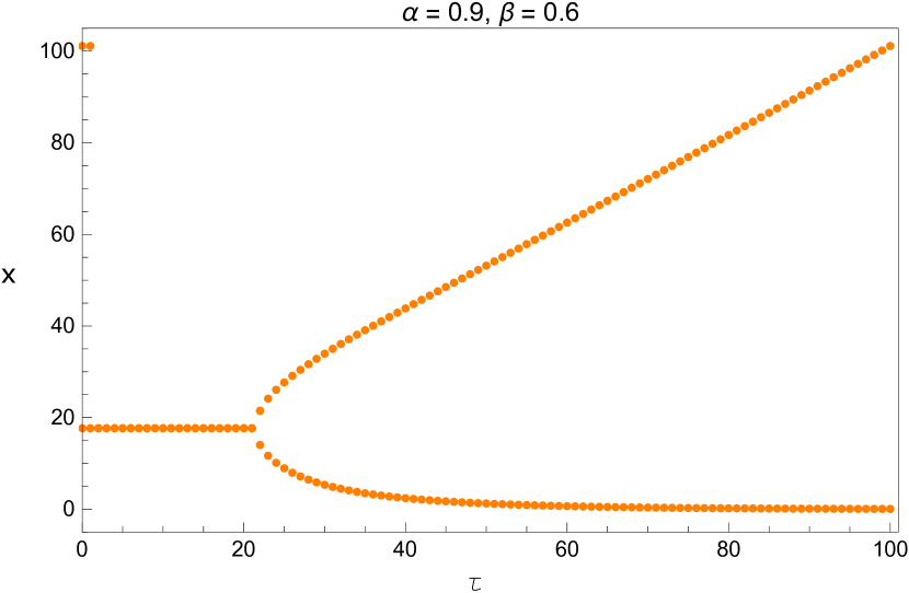
We now list the equilibrium point $(x_{*},y_{*})$ and critical delay $\tau_{*}$ for these combinations of $\alpha$ and $\beta.$

Table 5: The equilibrium point and critical delay for various values of

\alpha

and

\beta

$\alpha$	$\beta$	$(x_{},y_{})$	$\tau_{*}$
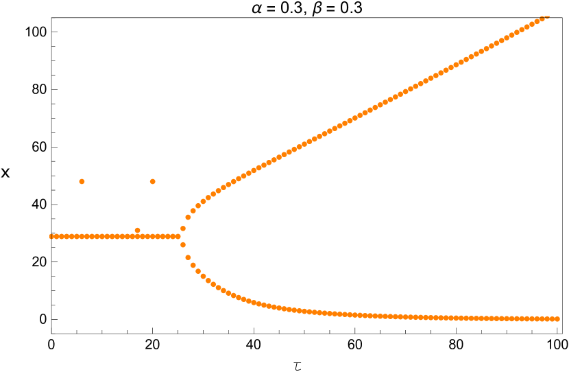
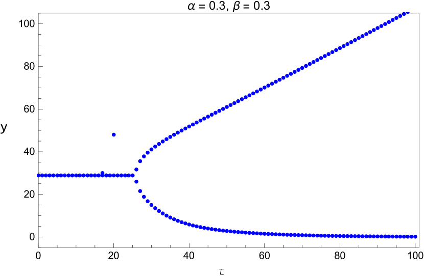
0.3	0.3	(28.8782, 28.8782)	25.8012
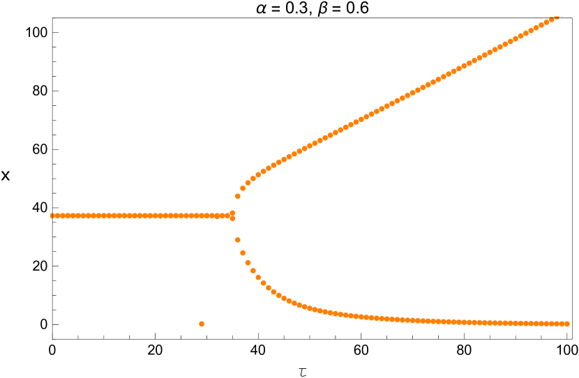
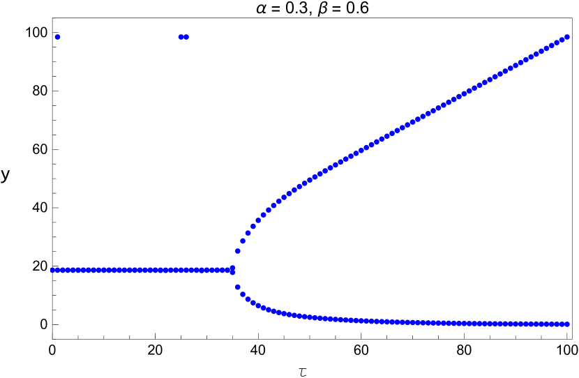
0.3	0.6	(37.2949, 18.6474)	35.1706
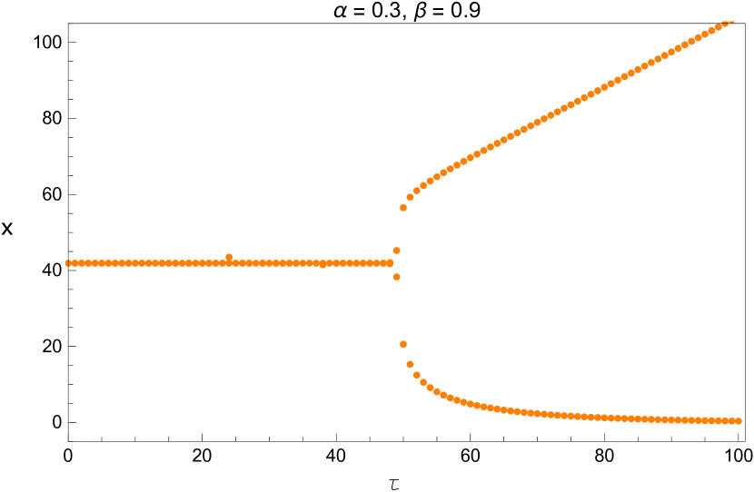
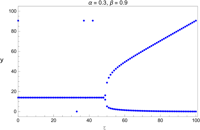
0.3	0.9	(41.9183, 13.9728)	49.4039
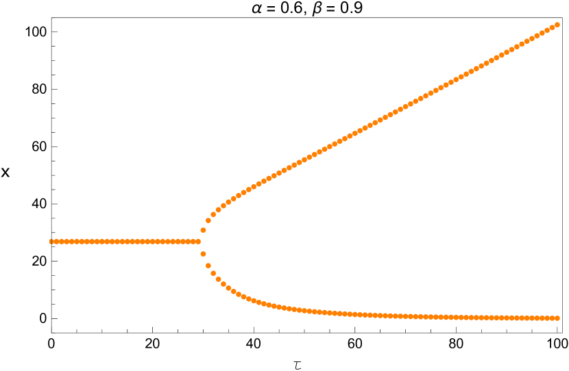
0.6	0.3	(17.5118, 35.0237)	20.5978
0.6	0.6	(23.4108, 23.4108)	24.9072
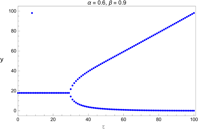
0.6	0.9	(26.8631, 17.9087)	29.6255
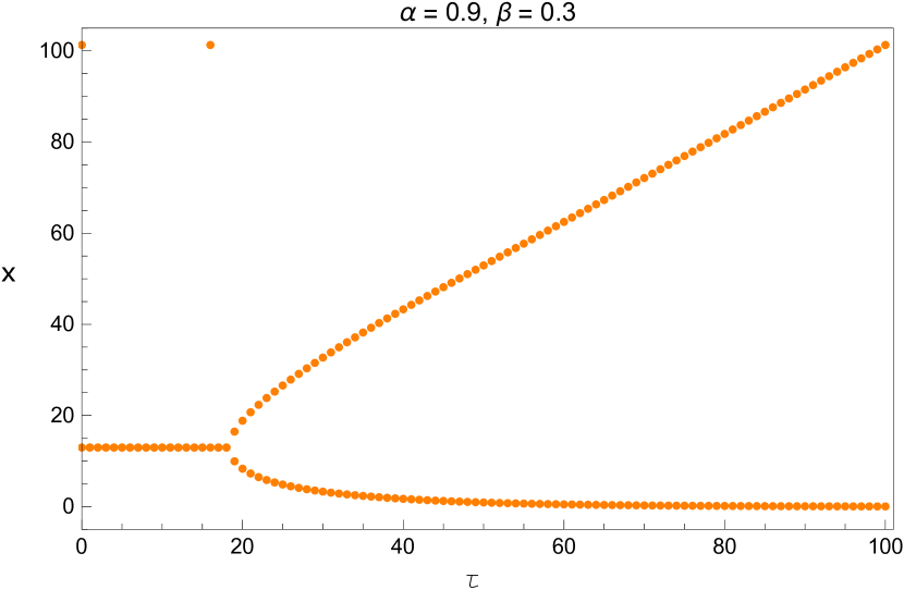
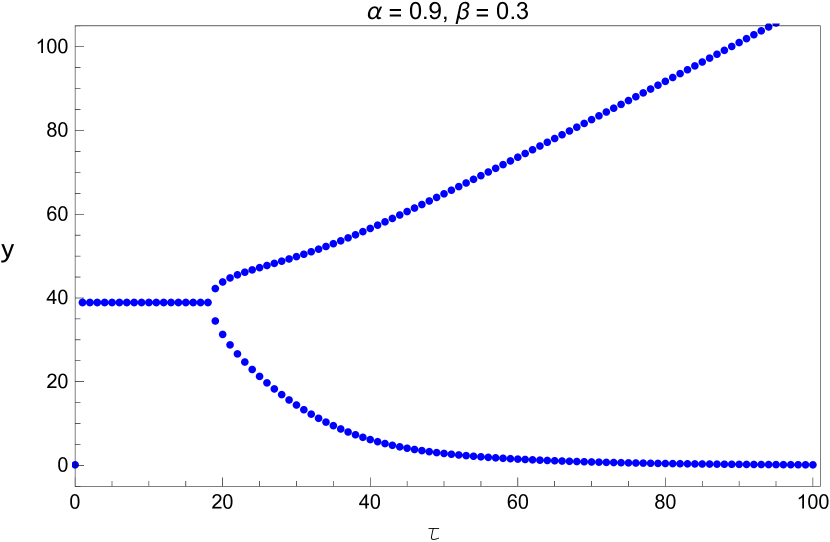
0.9	0.3	(12.9723, 38.9169)	18.3737
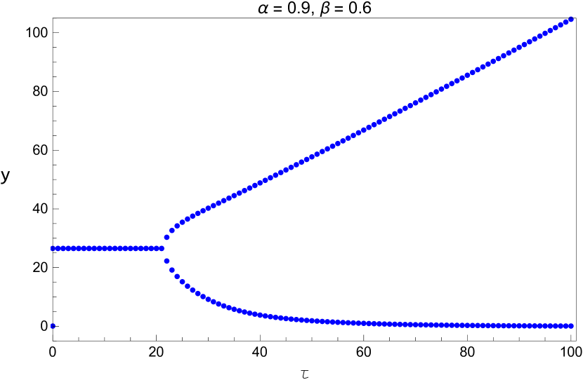
0.9	0.6	(17.6832, 26.5248)	21.4466
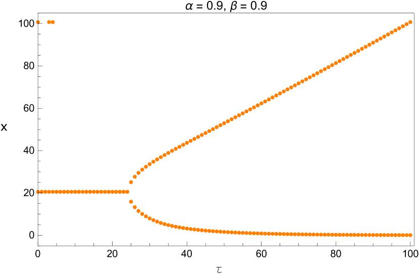
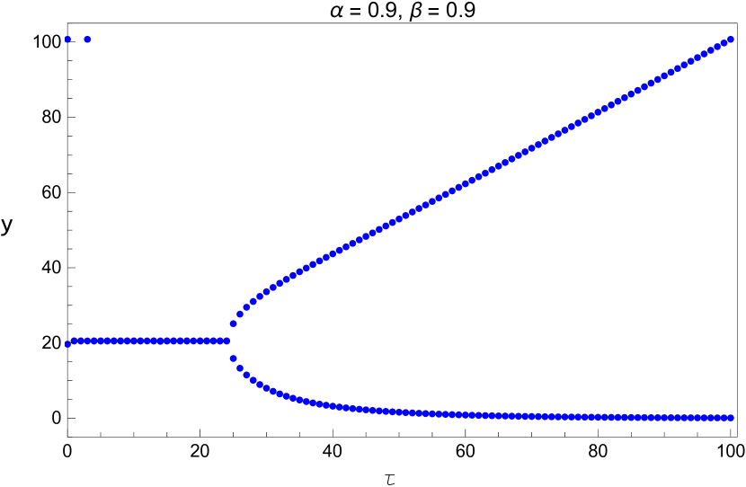
0.9	0.9	(20.5381, 20.5381)	24.3089

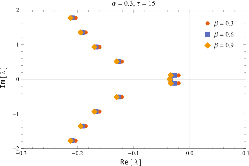
In figure 10, the characteristic roots of the smallest modulus are shown for the default values of $\alpha=0.5,$ and $\beta=0.8$ while varying the parameter $\tau$ near the critical delay.

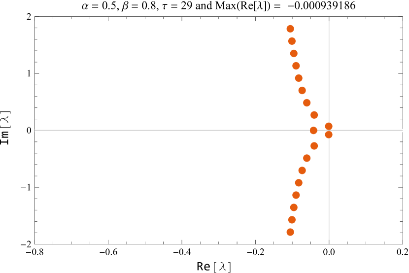
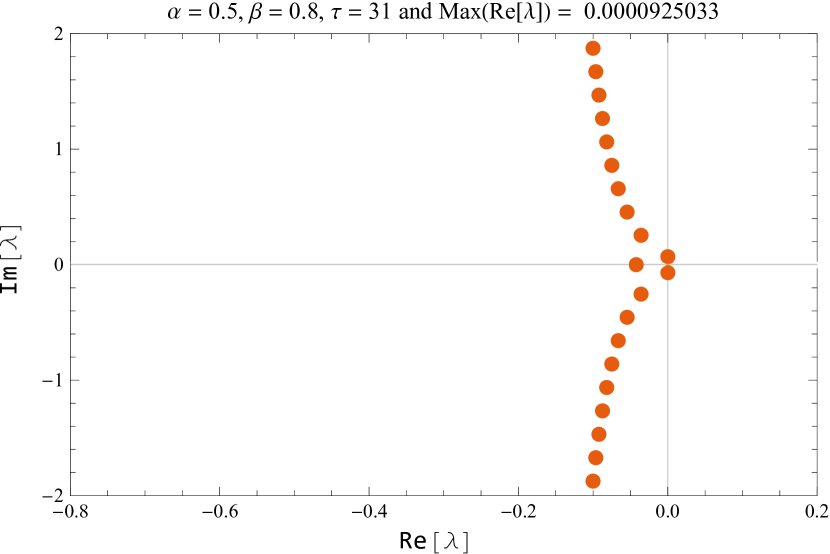
Figure 11 shows the characteristic roots of the smallest modulus for various parameters of $\alpha,$ $\beta$ and $\tau.$

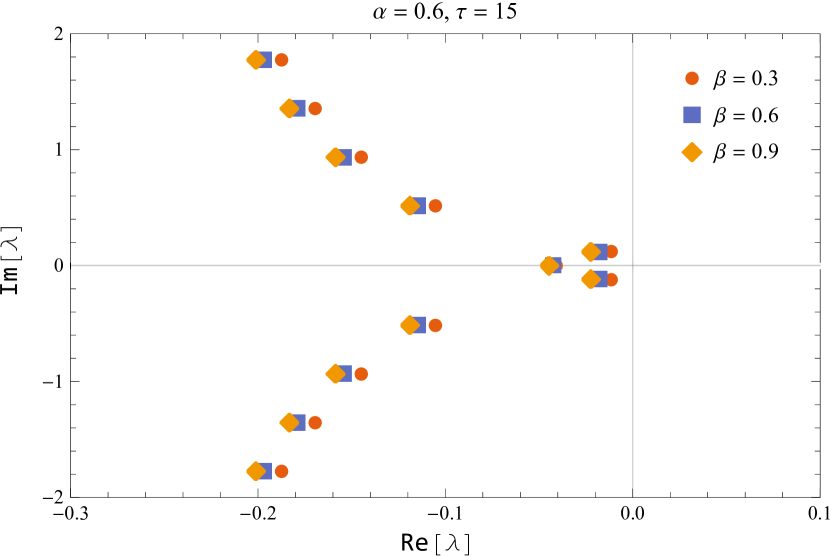
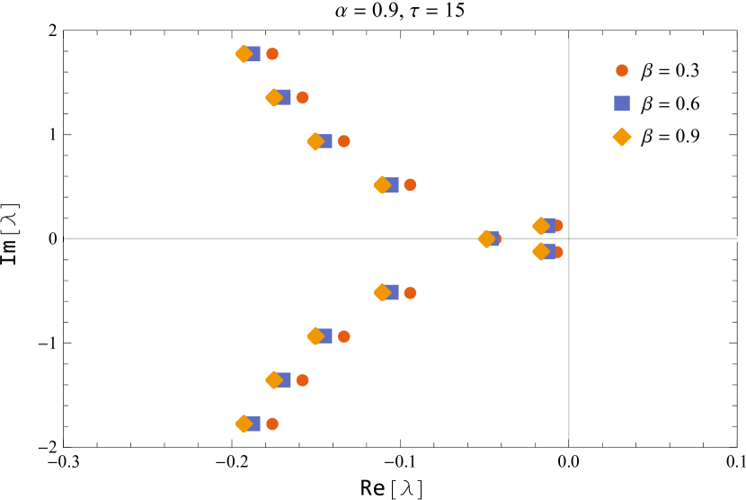
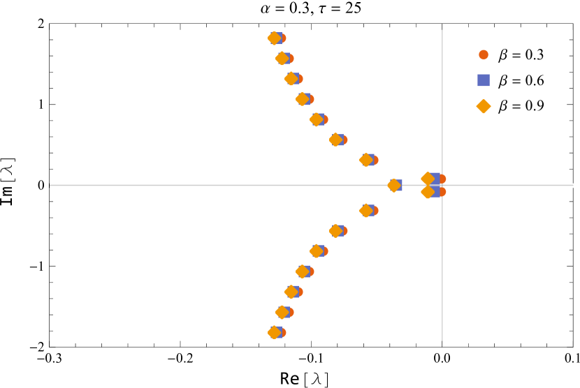
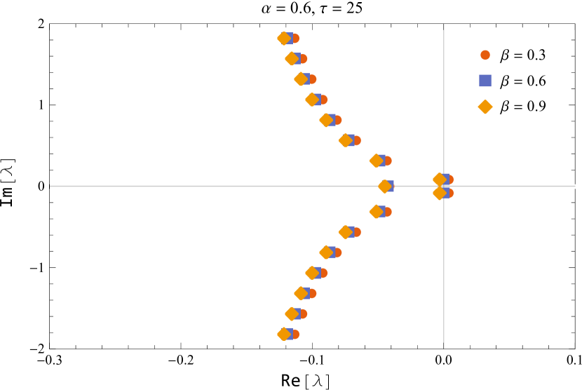
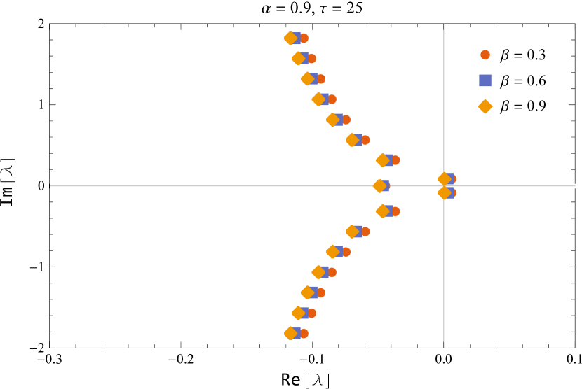
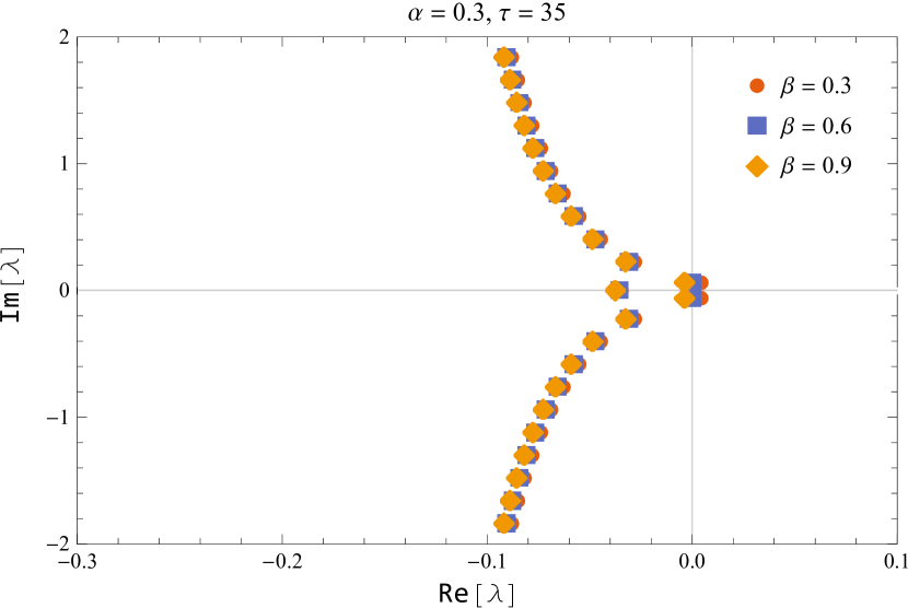
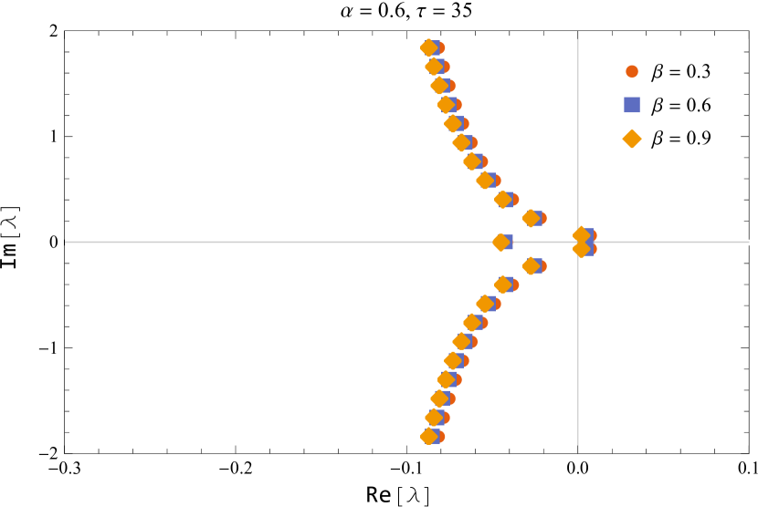
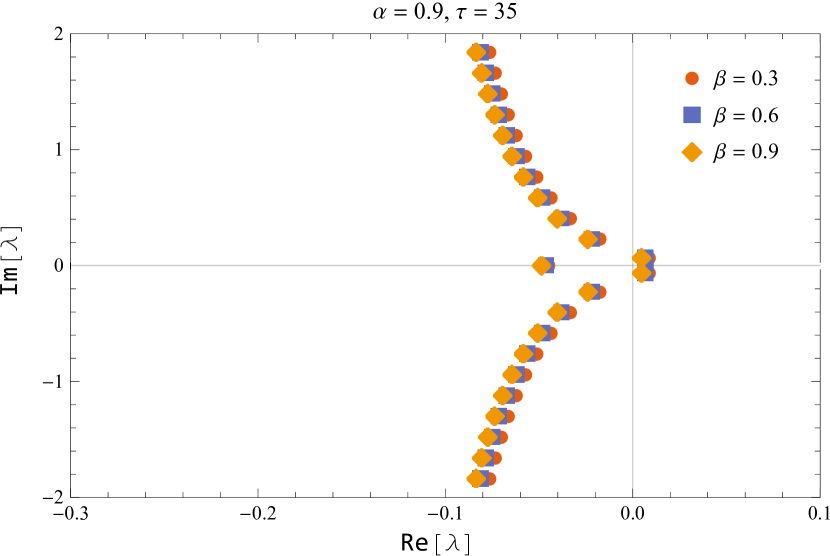
Thus, we deduced that the (5) is asymptotically stable for $0\leq\tau<\tau_{*}$ and unstable for $\tau>\tau_{*}$ , and undergoes a Hopf bifurcation at the positive equilibrium $E_{*}(x_{*},y_{*})$ for $\tau=\tau_{*}(n)$ for $n=0,1,2,\ldots$

2.4 Bifurcation Diagram

We vary the time delay $\tau$ with $\alpha=0.5$ and $\beta=0.8.$ When $\tau\geq 30.8017,$ the fixed point loses its stability through Hopf bifurcation as discussed in the previous section. The system (5) is run for a time span of [0 20,000] and we consider only the last one-fourth part to eliminate the possible transient responses. The bifurcation diagram is shown in Figure 12.

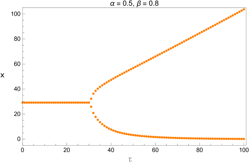
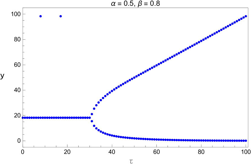
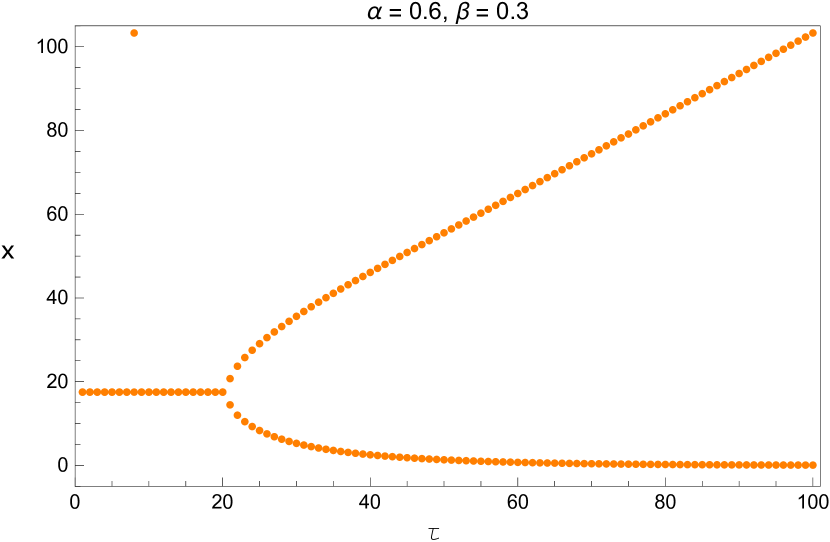
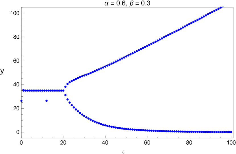
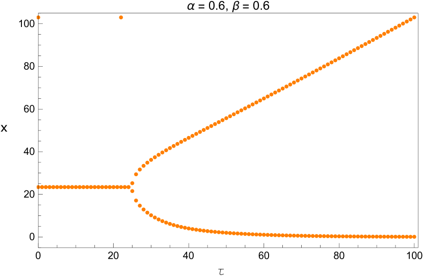
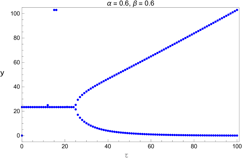
We also plot the bifurcation diagram of the long term values of the system with the parameters $\alpha$ and $\beta$ listed in Table 5. Since these diagrams are plotted by a different method, this provides us another opportunity to verify the values we found in that table. This is shown in Figures 13 - 15.

3 Direction and Stability of the Hopf Bifurcation

In this section, we apply the normal form theory and the center manifold theorem of Hassard et al [20] to get some properties of the Hopf bifurcation. In order to determine the direction and the stability of the Hopf bifurcation, we consider the following system whose equilibrium is shifted to the origin. Let $\tau=\tau_{*}+\mu$ , then $\mu=0$ is the Hopf bifurcation value of system (5) at the positive equilibrium $E(x_{*},y_{*})$ and $\pm i\omega_{*}$ is the corresponding purely imaginary roots of the characteristic equation.

For the convenience of discussion, let $x_{1}=x-x_{*}$ , $x_{2}=y-y_{*}$ . The system (5) can be regarded as FDE in $C=C([-1,0],\mathbb{R}^{2})$ as

\dot{x}=L_{\mu}(x_{t})+f(\mu,x_{t})

(33)

where $x(t)=(x_{1},x_{2})^{T}\in\mathbb{R}^{2}$ , and $L_{\mu}:C\to\mathbb{R}$ , $f:\mathbb{R}\times C\to\mathbb{R}$ are given respectively by

\begin{split}L_{\mu}(\phi)&=(\tau+\mu)\left(\begin{array}[]{cc}\frac{1}{25}(-7)\beta e^{\frac{\gamma}{20}-5}\gamma&-\frac{7\beta^{2}e^{\frac{\gamma}{20}-5}\gamma^{2}}{1000\alpha}\\ \frac{1}{50}(-7)\beta e^{\frac{\gamma}{20}-5}\gamma&-\frac{7\beta^{2}e^{\frac{\gamma}{20}-5}\gamma(\gamma+20)}{1000\alpha}\\ \end{array}\right)\begin{pmatrix}\phi_{1}(0)\\ \phi_{2}(0)\\ \end{pmatrix}\\ &+(\tau+\mu)\left(\begin{array}[]{cc}\frac{1}{50}(-7)\alpha e^{\frac{\gamma}{20}-5}x_{*}&-\frac{7\beta e^{\frac{\gamma}{20}-5}\gamma x_{*}}{1000}\\ \frac{1}{50}(-7)\beta e^{\frac{\gamma}{20}-5}y_{*}&-\frac{7\beta^{2}e^{\frac{\gamma}{20}-5}\gamma y_{*}}{1000\alpha}\\ \end{array}\right)\begin{pmatrix}\phi_{1}(-1)\\ \phi_{2}(-1)\\ \end{pmatrix}\end{split}

(34)

and

f(\mu,\phi)=(\tau+\mu)\begin{pmatrix}-\frac{7\alpha}{50e^{5}}\phi_{1}^{2}(0)\\ -\frac{7\beta}{50e^{5}}\phi_{1}(-1)\phi_{2}(-1)\\ \end{pmatrix}

(35)

According to the Riesz representation theorem, there exists a matrix function $\eta(\vartheta,\mu),$ $\vartheta\in[-1,0]$ with bounded variation components such that

L_{\mu}(\phi)=\int_{-1}^{0}d\eta(\vartheta,0)\phi(\vartheta)\quad\text{for}\quad\phi\in C

(36)

Actually we can take

\begin{split}\eta(\vartheta,\mu)&=(\tau+\mu)\left(\begin{array}[]{cc}\frac{1}{25}(-7)\beta e^{\frac{\gamma}{20}-5}\gamma&-\frac{7\beta^{2}e^{\frac{\gamma}{20}-5}\gamma^{2}}{1000\alpha}\\ \frac{1}{50}(-7)\beta e^{\frac{\gamma}{20}-5}\gamma&-\frac{7\beta^{2}e^{\frac{\gamma}{20}-5}\gamma(\gamma+20)}{1000\alpha}\\ \end{array}\right)\delta(\vartheta)\\ &-(\tau+\mu)\left(\begin{array}[]{cc}\frac{1}{50}(-7)\alpha e^{\frac{\gamma}{20}-5}x_{*}&-\frac{7\beta e^{\frac{\gamma}{20}-5}\gamma x_{*}}{1000}\\ \frac{1}{50}(-7)\beta e^{\frac{\gamma}{20}-5}y_{*}&-\frac{7\beta^{2}e^{\frac{\gamma}{20}-5}\gamma y_{*}}{1000\alpha}\\ \end{array}\right)\delta(\vartheta+1)\end{split}

(37)

where $\delta$ is the Dirac Delta function. For $\phi\in C^{1}([-1,0],\mathbb{R}^{2})$ , define

A(\mu)\phi=\left\{\begin{array}[]{ll}\frac{d\phi(\vartheta)}{d\vartheta},&\vartheta\in[-1,0),\\ \int_{1}^{0}d\eta(\mu,s)\phi(s)&\vartheta=0,\end{array}\right.

(38)

and

R(\mu)\phi=\left\{\begin{array}[]{ll}0,&\vartheta\in[-1,0),\\ f(\mu,\phi)&\vartheta=0,\end{array}\right.

(39)

The system (33) can be represented as

\dot{x}=A_{\mu}(x_{t})+R(\mu)x_{t}

(40)

where $x_{t}(\vartheta)=x(t+\vartheta)$ for $\vartheta\in[-1,0].$

For $\psi\in C^{1}([0,1],(\mathbb{R}^{2})^{*}),$ define

A^{*}\psi(s)=\left\{\begin{array}[]{ll}-\frac{d\psi(s)}{ds},&s\in(0,1],\\ \int_{1}^{0}d\eta^{T}(t,0)\psi(-t)&s=0,\end{array}\right.

(41)

Furthermore, for $\phi\in C^{1}([-1,0],(\mathbb{R}^{2})^{*}),$ and $\psi\in C^{1}([0,1],(\mathbb{R}^{2})^{*}),$ we give the bilinear inner product as

\left<\psi(s),\phi(\vartheta)\right>=\bar{\psi}(0)\phi(0)-\int_{-1}^{0}\int_{\xi=0}^{\vartheta}\bar{\psi}(\xi-\vartheta)d\eta(\vartheta)\phi(\xi)d\xi

(42)

where $\eta(\vartheta)=\eta(\vartheta,0).$ Then $A(0)$ and $A^{*}$ are adjoint operators. From previous section, we have that $\pm i\omega_{*}\tau_{*}$ are eigenvalues of $A(0).$ It is evident that they are also the eigenvalues of the linear operator $A^{*}.$ We need to compute the eigenvectors of $A(0)$ and $A^{*}$ corresponding to $i\omega_{*}\tau_{*}$ and $-i\omega_{*}\tau_{*}.$

Assume that

q(\vartheta)=\begin{pmatrix}1\\ c\\ \end{pmatrix}e^{i\omega_{*}\tau_{*}\vartheta}

(43)

is the eigenvector of $A(0)$ corresponding to $i\omega_{*}\tau_{*}$ and when $\vartheta=0,$ we have

q(0)=\begin{pmatrix}1\\ c\\ \end{pmatrix}

(44)

Then

A(0)q(\vartheta)=i\omega_{*}\tau_{*}q(\vartheta)

(45)

From the definition of $A(0)$ and (33), (36) and (37), we get

A(0)q(0)=\begin{pmatrix}i\omega_{*}\tau_{*}\\ i\omega_{*}\tau_{*}c\\ \end{pmatrix}

(46)

or,

\tau_{*}\left(\begin{array}[]{cc}\frac{7}{25}\beta e^{\frac{\gamma}{20}-5}\gamma+\frac{7}{50}\alpha xe^{\frac{\gamma}{20}-i\tau\omega-5}+i\omega&\frac{7\beta^{2}e^{\frac{\gamma}{20}-5}\gamma^{2}}{1000\alpha}+\frac{7\beta\gamma xe^{\frac{\gamma}{20}-i\tau\omega-5}}{1000}\\ \frac{7}{50}\beta e^{\frac{\gamma}{20}-5}\gamma+\frac{7}{50}\beta ye^{\frac{\gamma}{20}-i\tau\omega-5}&\frac{7\beta^{2}e^{\frac{\gamma}{20}-5}\gamma(\gamma+20)}{1000\alpha}+\frac{7\beta^{2}\gamma ye^{\frac{\gamma}{20}-i\tau\omega-5}}{1000\alpha}+i\omega\\ \end{array}\right).

(47)

q(0)=\left(\begin{array}[]{c}0\\ 0\\ \end{array}\right)

Thus we obtain,

c=-\frac{140\alpha\beta e^{\gamma/20}\left(y+\gamma e^{i\tau\omega}\right)}{1000i\alpha\omega e^{5+i\tau\omega}+7\beta^{2}\gamma^{2}e^{\frac{\gamma}{20}+i\tau\omega}+140\beta^{2}\gamma e^{\frac{\gamma}{20}+i\tau\omega}+7\beta^{2}e^{\gamma/20}\gamma y}

(48)

Similarly, we can get the eigenvector

q^{*}(s)=D\begin{pmatrix}1\\ c^{*}\\ \end{pmatrix}e^{i\omega_{*}\tau_{*}s}

(49)

of $A^{*}$ corresponding to $-i\omega_{*}\tau_{*},$ where

c^{*}=\frac{50i\omega e^{-\frac{\gamma}{20}+i\tau\omega+5}-7\left(\alpha x+2\beta\gamma e^{i\tau\omega}\right)}{7\beta\left(y+\gamma e^{i\tau\omega}\right)}

(50)

Now we evaluate the value of $D$ such that $\left<q^{*}(s),q(\vartheta)\right>=1.$ From the bilinear inner product of (42), it follows that

$\displaystyle 1$	$\displaystyle=\left<q^{*}(s),q(\vartheta)\right>$	(51)
	$\displaystyle=\bar{q}^{}(0)q(0)-\int_{-1}^{0}\int_{\xi=0}^{\vartheta}\bar{q}^{}(\xi-\vartheta)d\eta(\vartheta)q(\xi)d\xi$
	$\displaystyle=\bar{D}(1,\bar{c}^{})(1,c)^{T}-\int_{-1}^{0}\int_{\xi=0}^{\vartheta}\bar{D}(1,\bar{c}^{})e^{-i\omega_{}\tau_{}(\xi-\vartheta)}d\eta(\vartheta)(1,c)^{T}e^{i\omega_{}\tau_{}\xi}d\xi$
	$\displaystyle=\bar{D}(1,\bar{c}^{})(1,c)^{T}-\bar{D}(1,\bar{c}^{})\int_{-1}^{0}\int_{\xi=0}^{\vartheta}d\eta(\vartheta)(1,c)^{T}e^{i\omega_{}\tau_{}\vartheta}d\xi$
	$\displaystyle=\bar{D}(1,\bar{c}^{})(1,c)^{T}-\bar{D}(1,\bar{c}^{})\int_{-1}^{0}\vartheta e^{i\omega_{}\tau_{}\vartheta}d\eta(\vartheta)(1,c)^{T}$
	$\displaystyle=\bar{D}\left\{1+c\bar{c}^{}+\bar{c}^{}\tau_{}\left(-\frac{7e^{\frac{\gamma}{20}-5}(20\alpha+\beta c\gamma)\left(\beta c^{}y_{}+\alpha x_{}\right)}{1000\alpha}\right)e^{-i\omega_{}\tau_{}}\right\}$

Thus, we have

\bar{D}=\frac{1}{1+c\bar{c}^{*}+\bar{c}^{*}\tau_{*}\left(-\frac{7e^{\frac{\gamma}{20}-5}(20\alpha+\beta c\gamma)\left(\beta c^{*}y_{*}+\alpha x_{*}\right)}{1000\alpha}\right)e^{-i\omega_{*}\tau_{*}}}

(52)

In addition, from $\left<\psi,A\phi\right>=\left<A^{*}\psi,\phi\right>$ and $A\bar{q}(\vartheta)=-i\omega_{*}\tau_{*}\bar{q}(\vartheta),$ we can obtain

$\displaystyle-i\omega_{}\tau_{}\left<q^{*},\bar{q}\right>$	$\displaystyle=\left<q^{*},A\bar{q}\right>$	(53)
	$\displaystyle=\left<A^{}q^{},\bar{q}\right>$
	$\displaystyle=\left<A^{}q^{},\bar{q}\right>$
	$\displaystyle=i\omega_{}\tau_{}\left<q^{*},\bar{q}\right>$

Hence $\left<q^{*}(s),\bar{q}(\vartheta)\right>=0.$

In rest of the section, we calculate the coordinates to describe the center manifold $C_{0}$ at $\mu=0$ by the method used in Hassard paper. Let $x_{t}$ be the solution of equation (40) and define $z(t)=\left<q^{*},x_{t}\right>;$ then

$\displaystyle\dot{z}(t)$	$\displaystyle=\left<q^{},\dot{x}_{t}\right>=\left<q^{},A(0)\dot{x}_{t}+R(0)x_{t}\right>$	(54)
	$\displaystyle=\left<q^{},A(0)\dot{x}_{t}\right>+\left<q^{},R(0)x_{t}\right>$
	$\displaystyle=\left<A^{}(0)q^{},\dot{x}_{t}\right>+\bar{q}^{*}(0)f_{0}(z,\bar{z})$
	$\displaystyle=i\omega_{}\tau_{}z+g(z,\bar{z})$

where

g(z,\bar{z})=\bar{q}^{*}(0)f_{0}(z,\bar{z})=g_{20}\frac{z^{2}}{2}+g_{11}z\bar{z}+g_{02}\frac{\bar{z}^{2}}{2}+g_{21}\frac{z^{2}\bar{z}}{2}+\ldots

(55)

Let

	$\displaystyle W(t,\vartheta)$	$\displaystyle=x_{t}(\vartheta)-z(t)q(\vartheta)-\bar{z}(t)\bar{g}(\vartheta)$		(56)
		$\displaystyle=x_{t}(\vartheta)-2\text{Re}\left\{z(t)q(\vartheta)\right\}$		(56)

On the center manifold $C_{0},$ we have

W(t,\vartheta)=W(z(t),\bar{z}(t),\vartheta),

(57)

where

W(z,\bar{z},\vartheta)=W_{20}(\vartheta)\frac{z^{2}}{2}+W_{11}(\vartheta)z\bar{z}+W_{02}(\vartheta)\frac{\bar{z}^{2}}{2}+W_{30}(\vartheta)\frac{z^{3}}{6}+\ldots

(58)

$z$ and $\bar{z}$ are local coordinates for center manifold $C_{0}$ in the direction of $q^{*}$ and $\bar{q}^{*}.$ Note that $W$ is real if $x_{t}$ is real. We only consider real solutions.

It follows from (56) and (58) that

$\displaystyle x_{t}(\vartheta)$	$\displaystyle=(x_{1t}(\vartheta),x_{2t}(\vartheta))^{T}$	(59)
	$\displaystyle=W(t,\vartheta)+2\text{Re}\left\{z(t)q(\vartheta)\right\}$
	$\displaystyle=W(t,\vartheta)+z(t)q(\vartheta)+\bar{z}(t)\bar{q}(\vartheta)$
	$\displaystyle=W_{20}(\vartheta)\frac{z^{2}}{2}+W_{11}(\vartheta)z\bar{z}+W_{02}(\vartheta)\frac{\bar{z}^{2}}{2}$
	$\displaystyle\quad+(1,c)^{T}e^{i\omega_{}\tau_{}\vartheta}z+(1,\bar{c})^{T}e^{-i\omega_{}\tau_{}\vartheta}\bar{z}+\ldots$

From (35), it follows that

	$\displaystyle q(z,\bar{z})$	$\displaystyle=\bar{q}^{*}(0)f(0,x_{t})$		(60)
		$\displaystyle=\tau_{}\bar{D}(1,\bar{c}^{})\begin{pmatrix}-\frac{7\alpha}{50e^{5}}x_{1t}^{2}(0)\\ -\frac{7\beta}{50e^{5}}x_{1t}(-1)x_{2t}(-1)\\ \end{pmatrix}$		(60)

and with

$\displaystyle x_{1t}(0)$	$\displaystyle=z+\bar{z}+W_{20}^{1}(0)\frac{z^{2}}{2}+W_{11}^{1}(0)z\bar{z}+W_{02}^{1}(0)\frac{\bar{z}^{2}}{2}+\dots$	(61)
$\displaystyle x_{1t}(-1)$	$\displaystyle=ze^{-i\tau_{}\omega_{}}+\bar{z}e^{i\tau_{}\omega_{}}+W_{20}^{1}(0)\frac{z^{2}}{2}+W_{11}^{1}(0)z\bar{z}+W_{02}^{1}(0)\frac{\bar{z}^{2}}{2}+\dots$
$\displaystyle x_{2t}(-1)$	$\displaystyle=zce^{-i\tau_{}\omega_{}}+\bar{z}\bar{c}e^{i\tau_{}\omega_{}}+W_{20}^{2}(0)\frac{z^{2}}{2}+W_{11}^{2}(0)z\bar{z}+W_{02}^{2}(0)\frac{\bar{z}^{2}}{2}+\dots$

we get,

$\displaystyle q(z,\bar{z})$	$\displaystyle=\tau_{*}\bar{D}\left\{-\frac{7\alpha}{50e^{5}}\left(z+\bar{z}+W_{20}^{1}(0)\frac{z^{2}}{2}+W_{11}^{1}(0)z\bar{z}+W_{02}^{1}(0)\frac{\bar{z}^{2}}{2}+\dots\right)^{2}\right.$	(62)
	$\displaystyle\quad-\frac{7\beta\bar{c}^{}}{50e^{5}}\left(ze^{-i\tau_{}\omega_{}}+\bar{z}e^{i\tau_{}\omega_{*}}+W_{20}^{1}(0)\frac{z^{2}}{2}+W_{11}^{1}(0)z\bar{z}+W_{02}^{1}(0)\frac{\bar{z}^{2}}{2}+\dots\right)$
	$\displaystyle\quad\times\left.\left(zce^{-i\tau_{}\omega_{}}+\bar{z}\bar{c}e^{i\tau_{}\omega_{}}+W_{20}^{2}(0)\frac{z^{2}}{2}+W_{11}^{2}(0)z\bar{z}+W_{02}^{2}(0)\frac{\bar{z}^{2}}{2}+\dots\right)\right\}$

Comparing the coefficients with (55), we have

$\displaystyle g_{20}$	$\displaystyle=2\tau_{}\bar{D}\left\{-\frac{7\alpha}{50e^{5}}-\frac{7}{50}\beta c\bar{c}^{}e^{-5-2i\tau_{}\omega_{}}\right\}$	(63)
$\displaystyle g_{11}$	$\displaystyle=2\tau_{}\bar{D}\left\{-\frac{7\alpha}{25e^{5}}-\frac{7\beta\bar{c}^{}\text{Re}\{c\}}{50e^{5}}\right\}$
$\displaystyle g_{02}$	$\displaystyle=2\tau_{}\bar{D}\left\{-\frac{7\alpha}{50e^{5}}-\frac{7}{50}\beta\bar{c}\bar{c}^{}e^{-5+2i\tau_{}\omega_{}}\right\}$
$\displaystyle g_{21}$	$\displaystyle=\tau_{}\bar{D}\left\{-\frac{7\alpha\left(4W_{11}^{1}(0)+2W_{20}^{1}(0)\right)}{50e^{5}}-\frac{7}{50}\beta\bar{c}^{}e^{-5-i\tau_{}\omega_{}}\times\right.$
	$\displaystyle\quad\left(e^{2i\tau_{}\omega_{}}\left(W_{20}^{1}(-1)\bar{c}+W_{20}^{2}(-1)\right)+2cW_{11}^{1}(-1)+2W_{11}^{2}(-1)\right)\bigg{\}}$

Since we have $W_{20}(\vartheta)$ and $W_{11}(\vartheta)$ in $g_{21},$ we still need to calculate these terms. From (40) and (56), we get

	$\displaystyle\dot{W}=\dot{x_{t}}-\dot{z}-\dot{\bar{z}}\bar{q}$	$\displaystyle=\left\{\begin{array}[]{ll}AW-2\text{Re}\left\{\bar{q}^{}(0)f_{0q}(\vartheta)\right\},&\vartheta\in[-1,0),\\ AW-2\text{Re}\left\{\bar{q}^{}(0)f_{0q}(\vartheta)\right\}+f_{0},&\vartheta=0,\end{array}\right.$		(64)
		$\displaystyle\stackrel{{\scriptstyle\text{def}}}{{=}}AW+H(z,\bar{z},\vartheta),$		(64)

where

H(z,\bar{z},\vartheta)=H_{20}(\vartheta)\frac{z^{2}}{2}+H_{11}(\vartheta)z\bar{z}+H_{02}(\vartheta)\frac{\bar{z}^{2}}{2}+\ldots

(65)

Thus, we have

AW(t,\vartheta)-\dot{W}=-H(z,\bar{z},\vartheta)=-H_{20}(\vartheta)\frac{z^{2}}{2}-H_{11}(\vartheta)z\bar{z}-H_{02}(\vartheta)\frac{\bar{z}^{2}}{2}+\ldots

(66)

From (58), we obtain

$\displaystyle AW(t,\vartheta)$	$\displaystyle=AW_{20}(\vartheta)\frac{z^{2}}{2}+AW_{11}(\vartheta)z\bar{z}+AW_{02}(\vartheta)\frac{\bar{z}^{2}}{2}+AW_{30}(\vartheta)\frac{z^{3}}{6}+\ldots$	(67)
$\displaystyle\dot{W}$	$\displaystyle=W_{z}\dot{z}+W_{\bar{z}}\dot{\bar{z}}=W_{20}(\vartheta)z\dot{z}+W_{11}(\vartheta)(\dot{z}\bar{z}+z\dot{\bar{z}})+\ldots$
	$\displaystyle=2i\omega_{}\tau_{}W_{20}(\vartheta)\frac{z^{2}}{2}+\ldots$

Thus we have,

	$\displaystyle(A-2i\omega_{}\tau_{})W_{20}(\vartheta)$	$\displaystyle=-H_{20}(\vartheta),$		(68)
	$\displaystyle AW_{11}(\vartheta)$	$\displaystyle=-H_{11}(\vartheta)$		(68)

For $\vartheta\in[-1,0),$

H(z,\bar{z},\vartheta)=-\bar{q}^{*}(0)f_{0q}(\vartheta)-\bar{q}^{*}(0)f_{0}(\vartheta)=-g(z,\bar{z})q(\vartheta)-\bar{g}(z,\bar{z})\bar{q}(\vartheta)

(69)

Comparing the coefficients with (65), we get

	$\displaystyle H_{20}(\vartheta)$	$\displaystyle=-g_{20}q(\vartheta)-\bar{g}_{02}\bar{q}(\vartheta)$		(70)
	$\displaystyle H_{11}(\vartheta)$	$\displaystyle=-g_{11}q(\vartheta)-\bar{g}_{11}\bar{q}(\vartheta)$		(70)

From (68) and (70) and the definition of $A,$ it follows that

\dot{W}_{20}(\vartheta)=2i\omega_{*}\tau_{*}W_{20}(\vartheta)+g_{20}q(\vartheta)+\bar{g}_{02}\bar{q}(\vartheta)

(71)

Notice that

q(\vartheta)=\begin{pmatrix}1\\ c\\ \end{pmatrix}e^{i\omega_{*}\tau_{*}\vartheta},

(72)

W_{20}(\vartheta)=\frac{ig_{20}}{\omega_{*}\tau_{*}}q(0)e^{i\omega_{*}\tau_{*}\vartheta}+\frac{i\bar{g}_{02}}{3\omega_{*}\tau_{*}}\bar{q}(0)e^{-i\omega_{*}\tau_{*}\vartheta}+E_{1}e^{2i\omega_{*}\tau_{*}\vartheta}

(73)

where $E_{1}=\left(E_{1}^{(1)},E_{1}^{(2)}\right)\in\mathbb{R}^{2}$ is a two-dimensional constant vector.

Similarly from (68) and (70), we obtain

W_{11}(\vartheta)=-\frac{ig_{11}}{\omega_{*}\tau_{*}}q(0)e^{i\omega_{*}\tau_{*}\vartheta}+\frac{i\bar{g}_{11}}{\omega_{*}\tau_{*}}\bar{q}(0)e^{-i\omega_{*}\tau_{*}\vartheta}+E_{2}

(74)

where $E_{2}=\left(E_{2}^{(1)},E_{2}^{(2)}\right)\in\mathbb{R}^{2}$ is a two-dimensional constant vector.

Next, we need to compute $E_{1}$ and $E_{2}.$ From the definition of $A$ and (68), we obtain

\int_{-1}^{0}d\eta(\vartheta)W_{20}(\vartheta)=2i\omega_{*}\tau_{*}W_{20}(0)-H_{20}(0)

and

\int_{-1}^{0}d\eta(\vartheta)W_{11}(\vartheta)=-H_{11}(0)

(75)

where $\eta(\vartheta)=\eta(0,\vartheta).$

By (64), we have

H_{20}(0)=-g_{20}q(0)-\bar{g}_{02}\bar{q}(0)+2\tau_{*}\begin{pmatrix}-7\alpha/\left(50e^{5}\right)\\ \frac{-7}{50e^{5}}\beta ce^{-2i\tau_{*}\omega_{*}}\\ \end{pmatrix}

(76)

and

H_{11}(0)=-g_{11}q(0)-\bar{g}_{11}\bar{q}(0)+2\tau_{*}\begin{pmatrix}-7\alpha/\left(25e^{5}\right)\\ -7\beta\text{Re}\{c\}/\left(50e^{5}\right)\\ \end{pmatrix}

(77)

Substituting (73) and (76) into (75), and noticing that

\left(i\omega_{*}\tau_{*}I-\int_{-1}^{0}e^{i\omega_{*}\tau_{*}\vartheta}d\eta(\vartheta)\right)q(0)=0

(78)

and

\left(-i\omega_{*}\tau_{*}I-\int_{-1}^{0}e^{-i\omega_{*}\tau_{*}\vartheta}d\eta(\vartheta)\right)\bar{q}(0)=0

(79)

we obtain,

\left(2i\omega_{*}\tau_{*}I-\int_{-1}^{0}e^{2i\omega_{*}\tau_{*}\vartheta}d\eta(\vartheta)\right)E_{1}=2\tau_{*}\begin{pmatrix}-7\alpha/\left(50e^{5}\right)\\ \frac{-7}{50e^{5}}\beta ce^{-2i\tau_{*}\omega_{*}}\\ \end{pmatrix}

(80)

This leads to

\begin{pmatrix}\frac{7}{25}\beta e^{\frac{\gamma}{20}-5}\gamma+\frac{7}{50}\alpha x_{*}e^{\frac{\gamma}{20}-2i\tau_{*}\omega_{*}-5}+2i\omega_{*}&\frac{7\beta^{2}e^{\frac{\gamma}{20}-5}\gamma^{2}}{1000\alpha}+\frac{7\beta\gamma x_{*}e^{\frac{\gamma}{20}-2i\tau_{*}\omega_{*}-5}}{1000}\\ \frac{7}{50}\beta e^{\frac{\gamma}{20}-5}\gamma+\frac{7}{50}\beta y_{*}e^{\frac{\gamma}{20}-2i\tau_{*}\omega_{*}-5}&\frac{7\beta^{2}e^{\frac{\gamma}{20}-5}\gamma(\gamma+20)}{1000\alpha}+\frac{7\beta^{2}\gamma y_{*}e^{\frac{\gamma}{20}-2i\tau_{*}\omega_{*}-5}}{1000\alpha}+2i\omega_{*}\\ \end{pmatrix}

\times E_{1}=2\begin{pmatrix}-7\alpha/\left(50e^{5}\right)\\ \frac{-7}{50e^{5}}\beta ce^{-2i\tau_{*}\omega_{*}}\\ \end{pmatrix}

(81)

It follows that

E_{1}^{(1)}=\frac{2}{A}\left|\begin{array}[]{cc}-7\alpha/\left(50e^{5}\right)&\frac{7\beta^{2}e^{\frac{\gamma}{20}-5}\gamma^{2}}{1000\alpha}+\frac{7\beta\gamma x_{*}e^{\frac{\gamma}{20}-2i\tau_{*}\omega_{*}-5}}{1000}\\ \frac{-7}{50e^{5}}\beta ce^{-2i\tau_{*}\omega_{*}}&\frac{7\beta^{2}e^{\frac{\gamma}{20}-5}\gamma(\gamma+20)}{1000\alpha}+\frac{7\beta^{2}\gamma y_{*}e^{\frac{\gamma}{20}-2i\tau_{*}\omega_{*}-5}}{1000\alpha}+2i\omega_{*}\\ \end{array}\right|

(82)

and

E_{1}^{(2)}=\frac{2}{A}\left|\begin{array}[]{cc}\frac{7}{25}\beta e^{\frac{\gamma}{20}-5}\gamma+\frac{7}{50}\alpha x_{*}e^{\frac{\gamma}{20}-2i\tau_{*}\omega_{*}-5}+2i\omega_{*}&-7\alpha/\left(50e^{5}\right)\\ \frac{7}{50}\beta e^{\frac{\gamma}{20}-5}\gamma+\frac{7}{50}\beta y_{*}e^{\frac{\gamma}{20}-2i\tau_{*}\omega_{*}-5}&\frac{-7}{50e^{5}}\beta ce^{-2i\tau_{*}\omega_{*}}\\ \end{array}\right|

(83)

where $A=$

\left|\begin{array}[]{cc}\frac{7}{25}\beta e^{\frac{\gamma}{20}-5}\gamma+\frac{7}{50}\alpha x_{*}e^{\frac{\gamma}{20}-2i\tau_{*}\omega_{*}-5}+2i\omega_{*}&\frac{7\beta^{2}e^{\frac{\gamma}{20}-5}\gamma^{2}}{1000\alpha}+\frac{7\beta\gamma x_{*}e^{\frac{\gamma}{20}-2i\tau_{*}\omega_{*}-5}}{1000}\\ \frac{7}{50}\beta e^{\frac{\gamma}{20}-5}\gamma+\frac{7}{50}\beta y_{*}e^{\frac{\gamma}{20}-2i\tau_{*}\omega_{*}-5}&\frac{7\beta^{2}e^{\frac{\gamma}{20}-5}\gamma(\gamma+20)}{1000\alpha}+\frac{7\beta^{2}\gamma y_{*}e^{\frac{\gamma}{20}-2i\tau_{*}\omega_{*}-5}}{1000\alpha}+2i\omega_{*}\\ \end{array}\right|

Similarly, substituting (74) and (77) into (75), we get

\left(\begin{array}[]{cc}\frac{7}{50}\alpha e^{\frac{\gamma}{20}-5}x_{*}-\frac{7}{25}\beta e^{\frac{\gamma}{20}-5}\gamma&\frac{7\beta e^{\frac{\gamma}{20}-5}\gamma x_{*}}{1000}-\frac{7\beta^{2}e^{\frac{\gamma}{20}-5}\gamma^{2}}{1000\alpha}\\ \frac{7}{50}\beta e^{\frac{\gamma}{20}-5}y_{*}-\frac{7}{50}\beta e^{\frac{\gamma}{20}-5}\gamma&\frac{7\beta^{2}e^{\frac{\gamma}{20}-5}\gamma y_{*}}{1000\alpha}-\frac{7\beta^{2}e^{\frac{\gamma}{20}-5}\gamma(\gamma+20)}{1000\alpha}\\ \end{array}\right)

\times E_{2}=2\begin{pmatrix}-7\alpha/\left(25e^{5}\right)\\ -7\beta\text{Re}\{c\}/\left(50e^{5}\right)\\ \end{pmatrix}

(84)

It follows that

E_{2}^{(1)}=\frac{2}{B}\left|\begin{array}[]{cc}-7\alpha/\left(25e^{5}\right)&\frac{7\beta e^{\frac{\gamma}{20}-5}\gamma x_{*}}{1000}-\frac{7\beta^{2}e^{\frac{\gamma}{20}-5}\gamma^{2}}{1000\alpha}\\ -7\beta\text{Re}\{c\}/\left(50e^{5}\right)&\frac{7\beta^{2}e^{\frac{\gamma}{20}-5}\gamma y_{*}}{1000\alpha}-\frac{7\beta^{2}e^{\frac{\gamma}{20}-5}\gamma(\gamma+20)}{1000\alpha}\\ \end{array}\right|

(85)

and

E_{2}^{(2)}=\frac{2}{B}\left|\begin{array}[]{cc}\frac{7}{50}\alpha e^{\frac{\gamma}{20}-5}x_{*}-\frac{7}{25}\beta e^{\frac{\gamma}{20}-5}\gamma&-7\alpha/\left(25e^{5}\right)\\ \frac{7}{50}\beta e^{\frac{\gamma}{20}-5}y_{*}-\frac{7}{50}\beta e^{\frac{\gamma}{20}-5}\gamma&-7\beta\text{Re}\{c\}/\left(50e^{5}\right)\\ \end{array}\right|

(86)

where

B=\left|\begin{array}[]{cc}\frac{7}{50}\alpha e^{\frac{\gamma}{20}-5}x_{*}-\frac{7}{25}\beta e^{\frac{\gamma}{20}-5}\gamma&\frac{7\beta e^{\frac{\gamma}{20}-5}\gamma x_{*}}{1000}-\frac{7\beta^{2}e^{\frac{\gamma}{20}-5}\gamma^{2}}{1000\alpha}\\ \frac{7}{50}\beta e^{\frac{\gamma}{20}-5}y_{*}-\frac{7}{50}\beta e^{\frac{\gamma}{20}-5}\gamma&\frac{7\beta^{2}e^{\frac{\gamma}{20}-5}\gamma y_{*}}{1000\alpha}-\frac{7\beta^{2}e^{\frac{\gamma}{20}-5}\gamma(\gamma+20)}{1000\alpha}\\ \end{array}\right|

Thus, we can determine $W_{20}(\vartheta)$ and $W_{11}(\vartheta)$ from (73) and (74). Furthermore, $g_{21}$ in (63) can be expressed by the parameters and delay. Thus, we can compute the following values:

$\displaystyle c_{1}(0)$	$\displaystyle=\frac{i}{2\omega_{}\tau_{}}\left(g_{20}g_{11}-2\left\|g_{11}\right\|^{2}-\frac{\left\|g_{02}\right\|^{2}}{3}\right)+\frac{g_{21}}{2},$	(87)
$\displaystyle\mu_{2}$	$\displaystyle=-\frac{\text{Re}\left\{c_{1}(0)\right\}}{\text{Re}\left\{\lambda^{{}^{\prime}}(\tau_{*})\right\}},$
$\displaystyle\beta_{2}$	$\displaystyle=2\text{Re}\left\{c_{1}(0)\right\},$
$\displaystyle T_{2}$	$\displaystyle=-\frac{\text{Im}\left\{c_{1}(0)\right\}+\mu_{2}\text{Im}\left\{\lambda^{{}^{\prime}}(\tau_{})\right\}}{\omega_{}\tau_{*}}$

which determines the qualities of bifurcation periodic solution in the center manifold at the critical value $\tau_{*}.$

Here $\mu_{2}$ determines the direction of the Hopf bifurcation. If $\mu_{2}>0$ , then the bifurcation is supercritical and the bifurcation periodic solutions exist for $\tau>\tau_{*}.$ $\beta_{2}$ determines the stability of the bifurcation periodic solutions: it is asymptotically stable if $\beta_{2}<0.$ $T_{2}$ determines the period of the bifurcation periodic solutions; the period increases if $T_{2}>0.$

4 Numerical Simulations

In section 2, we derived that the positive equilibrium $E_{*}(x_{*},y_{*})$ is asymptotically stable for $0\leq\tau<\tau_{*}$ and unstable for $\tau>\tau_{*}$ and the system (5) undergoes a Hopf bifurcation when $\tau=\tau_{*}.$ Here we will give the dynamic behaviors of the system with different values of the parameters $\alpha$ and $\beta$ with different time delay $\tau.$ The simulation results of system (5) are plotted using the software Mathematica Version 12.1 [49].

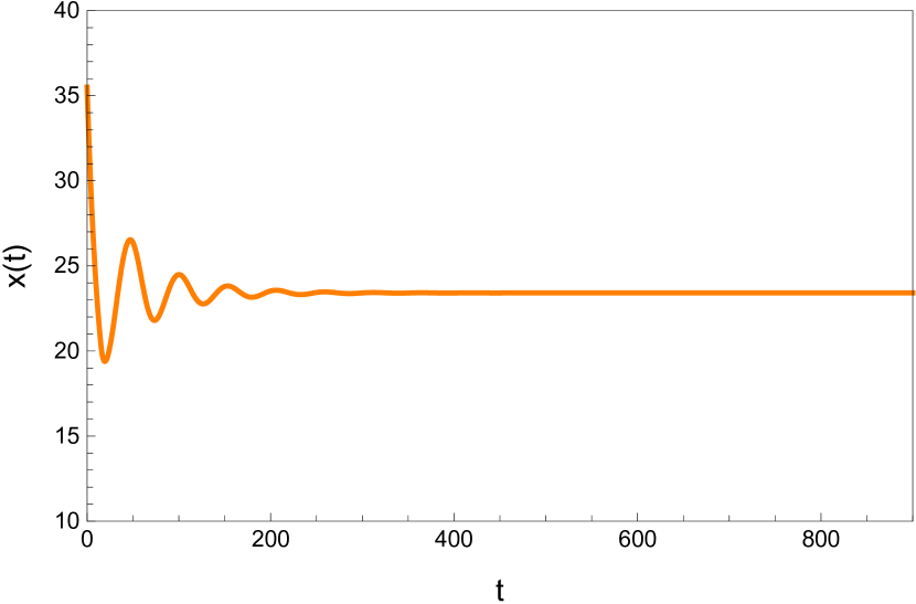
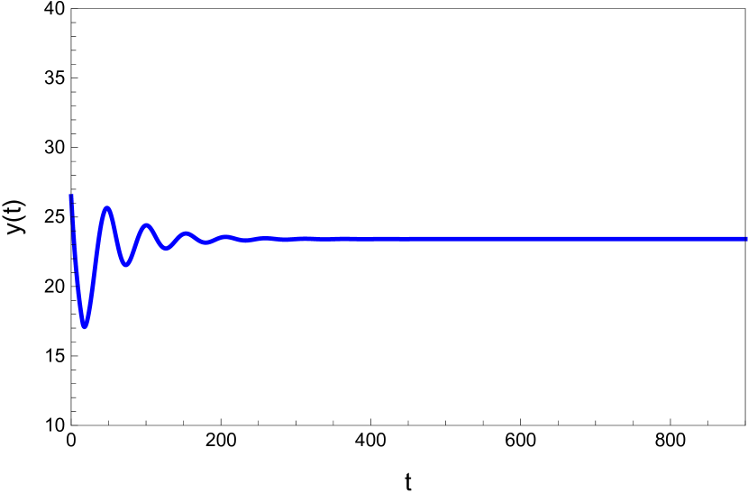
4.1 The dynamic behavior with $\alpha=0.5\textrm{ and }\beta=0.8$

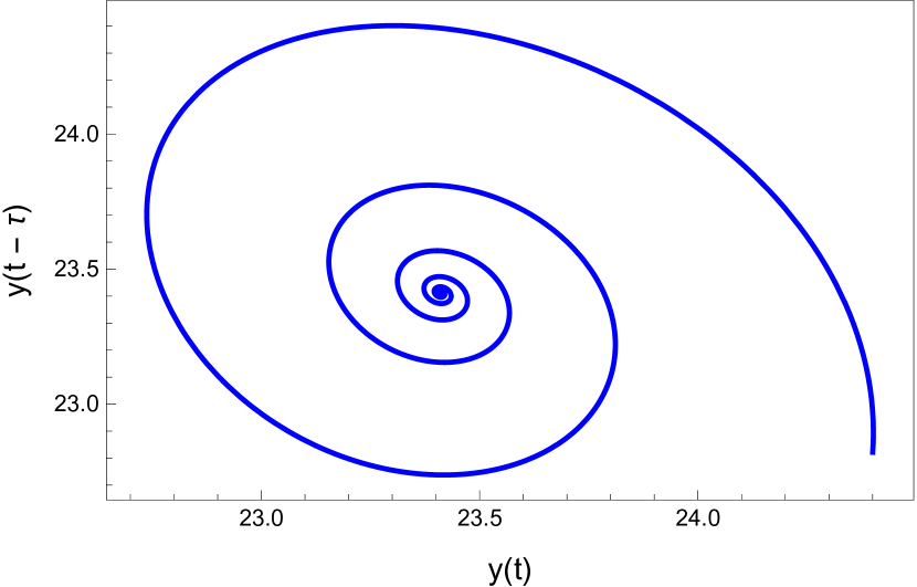
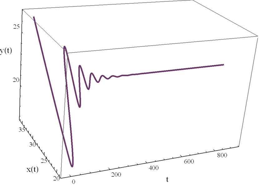
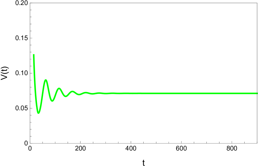
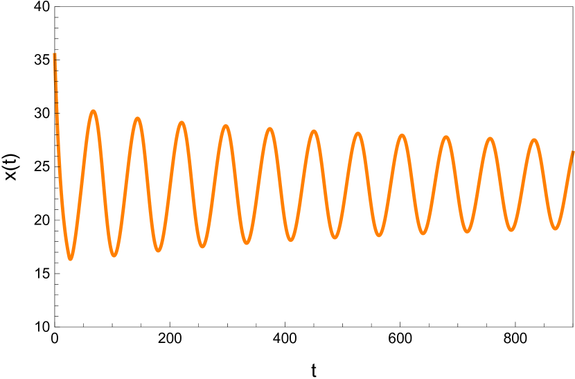
Here we study the dynamic behavior of system (5) by changing the time delay $\tau$ with $\alpha=0.5$ and $\beta=0.8.$ All the simulations have initial conditions of $x(t)=35.5$ and $y(t)=26.5.$ This has a unique positive equilibrium at $(x_{*},y_{*})=(29.1842,18.2401).$ We observe that the equilibrium is stable for $\tau<30.8017$ and unstable for $\tau>30.8017.$ At a Hopf bifurcation, no new equilibrium arise. A periodic solution emerges at the equilibrium point as $\tau$ passes through the bifurcation value.

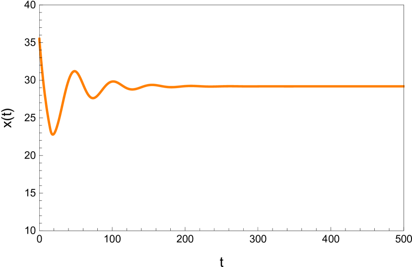
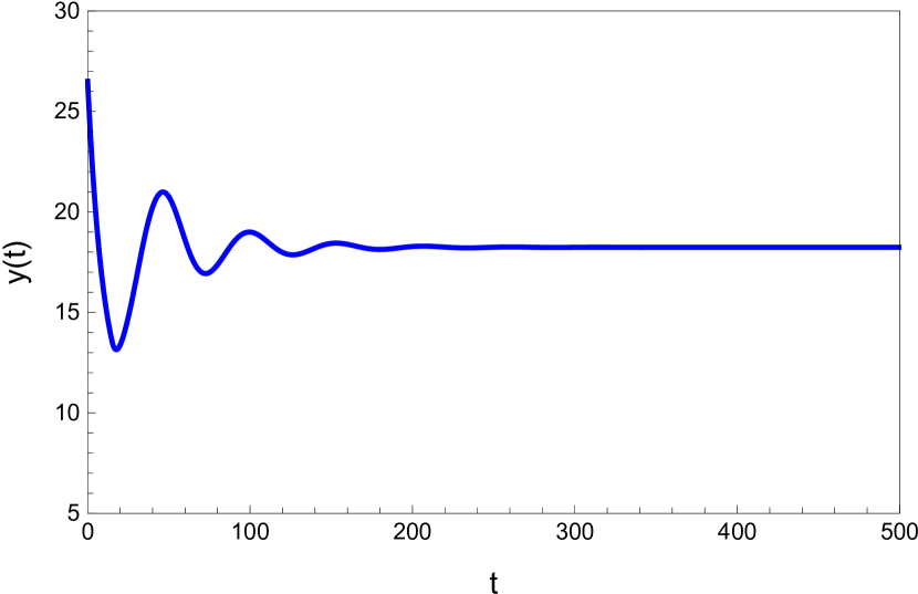
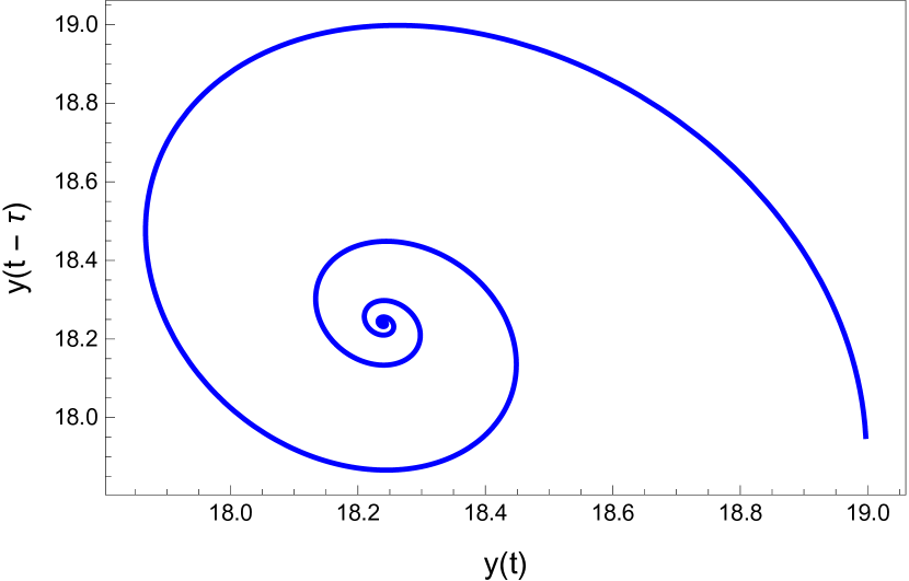
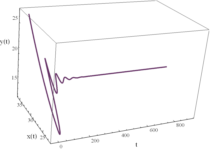
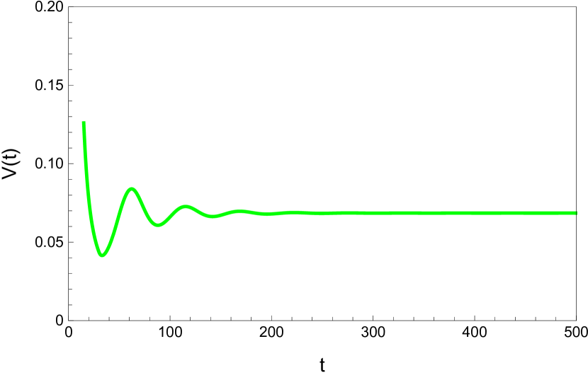
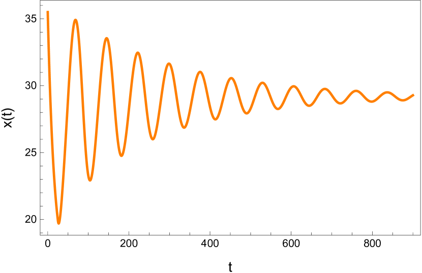
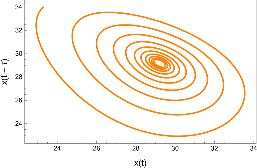
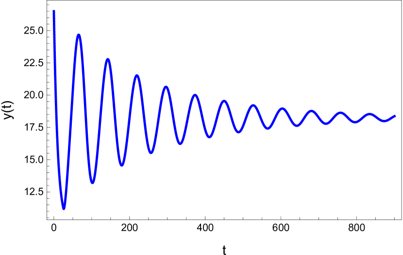
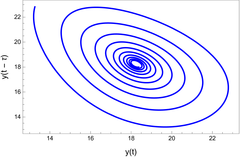
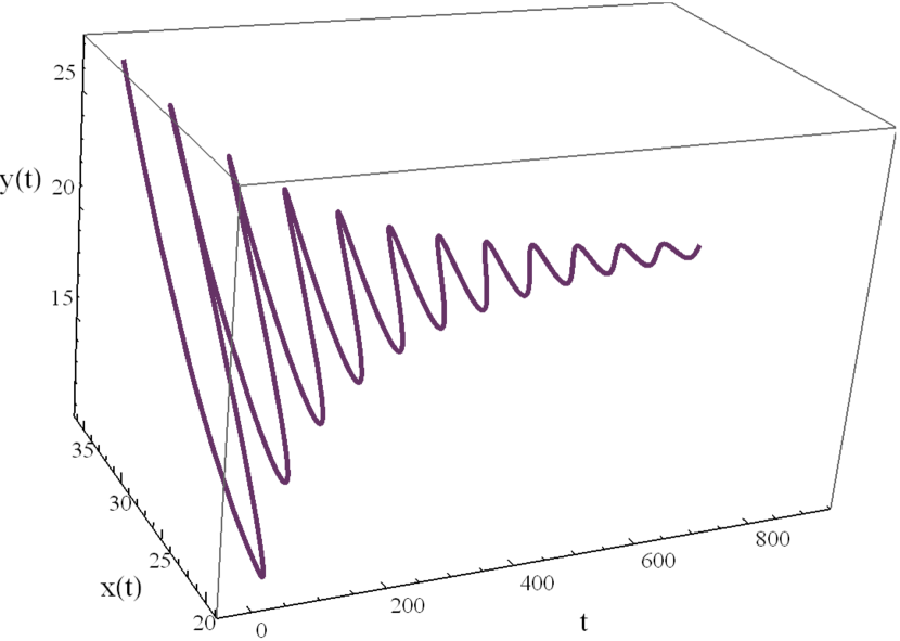
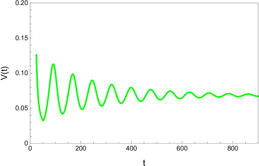
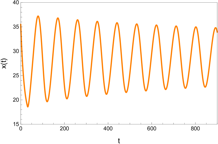
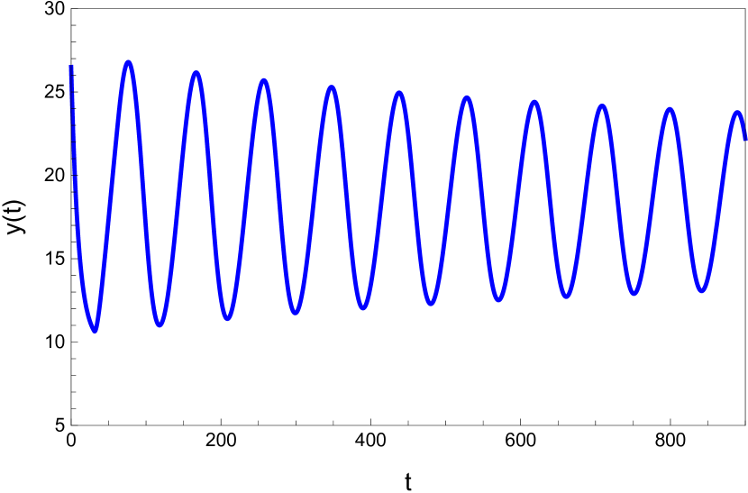
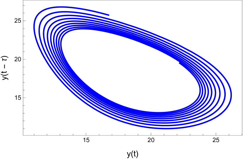
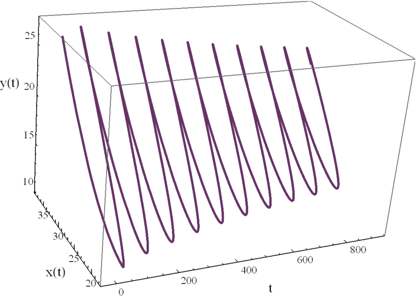
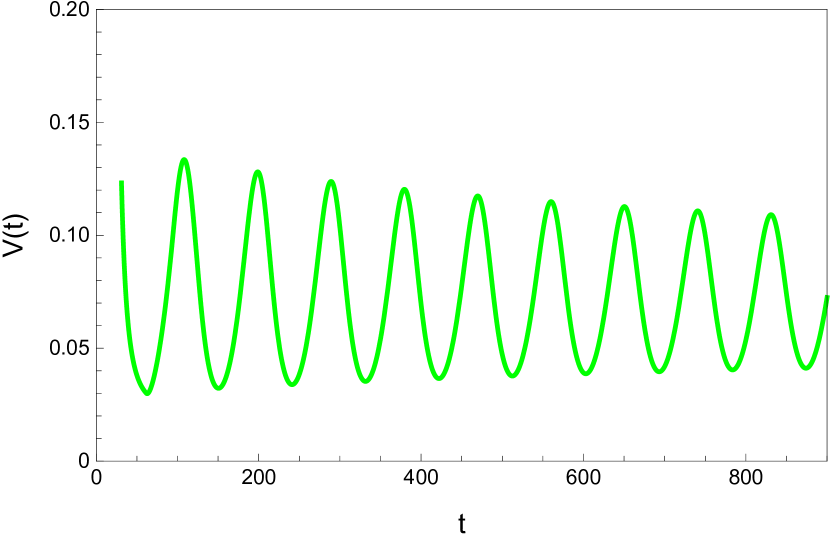
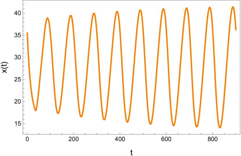
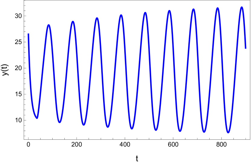
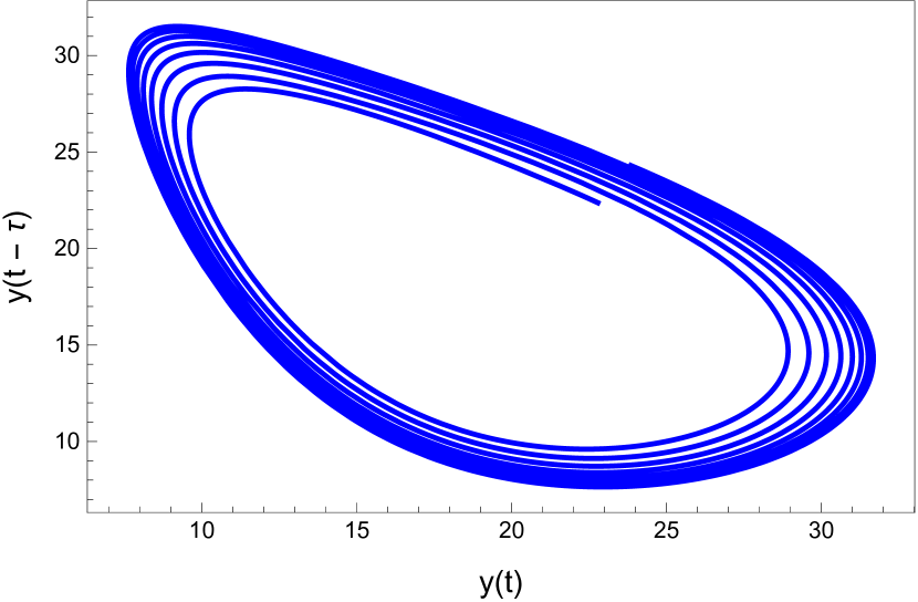
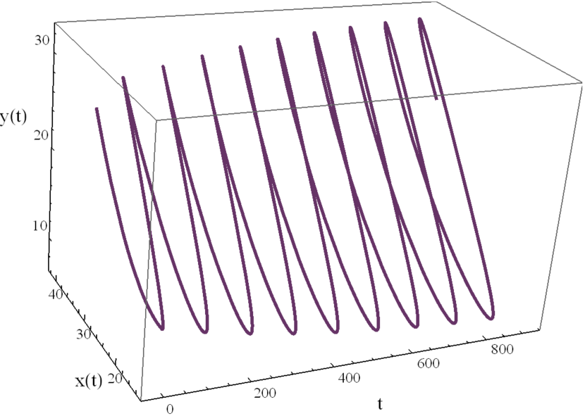
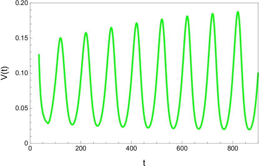
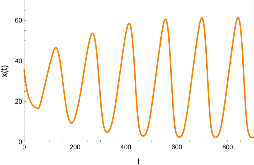
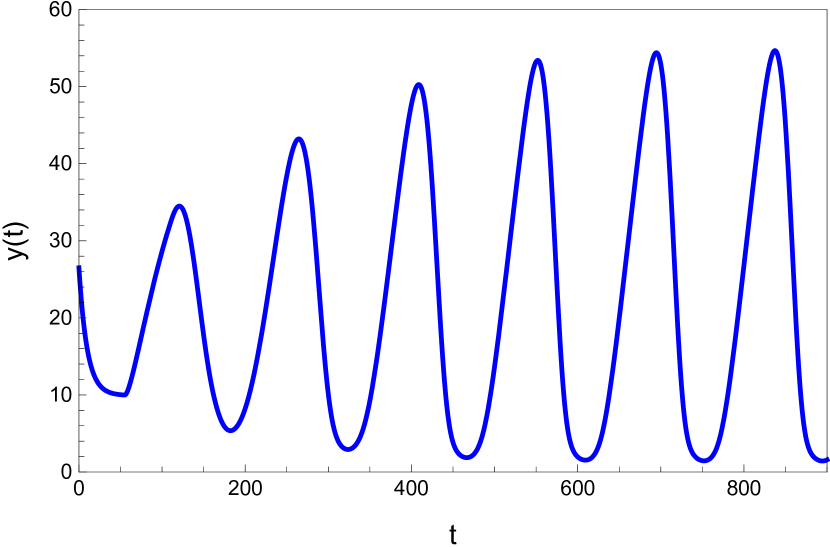
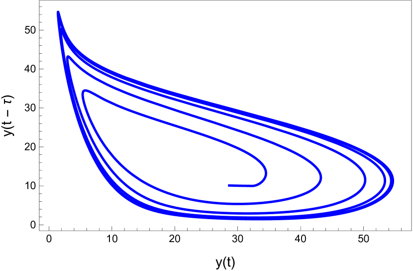
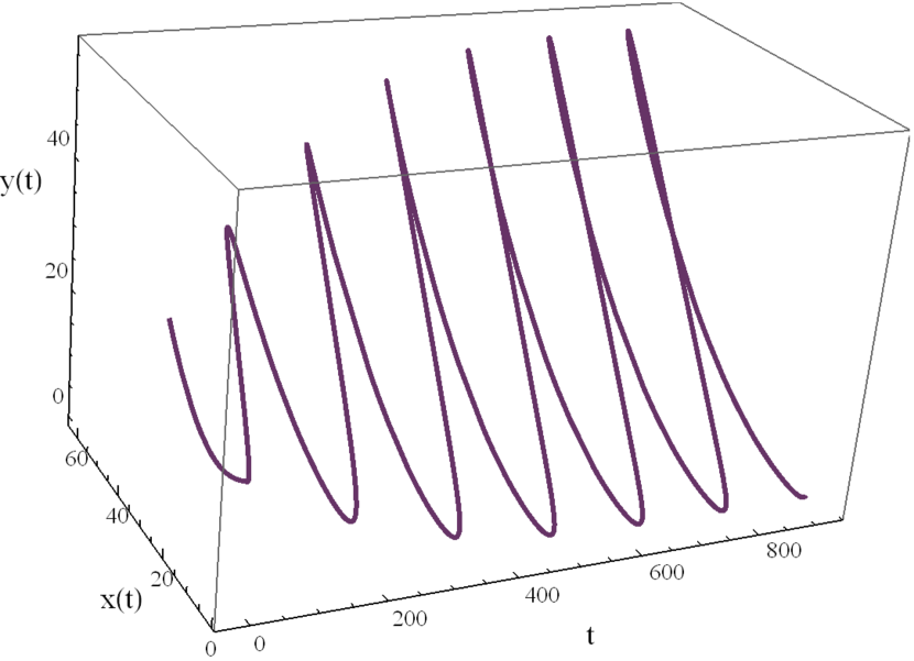
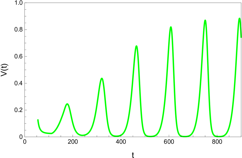
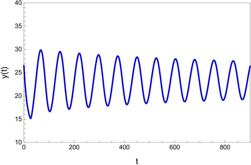
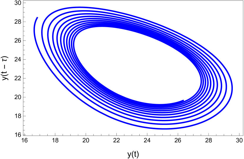
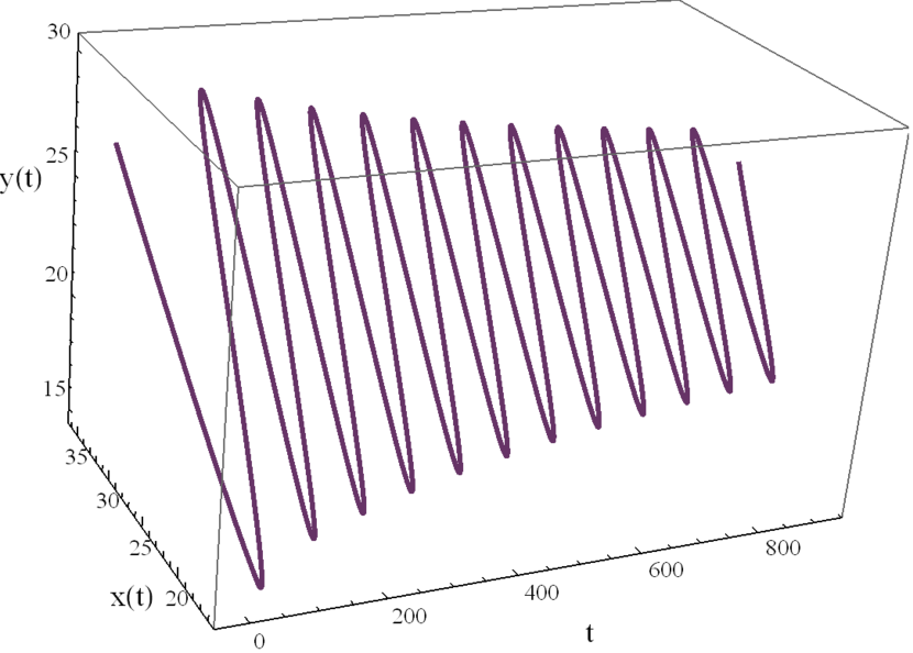
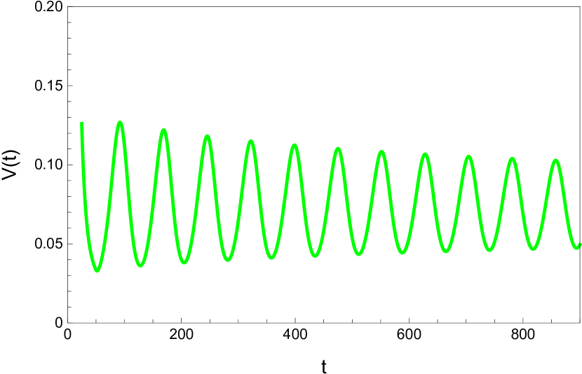
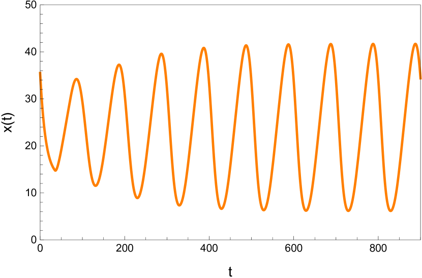
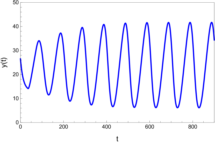
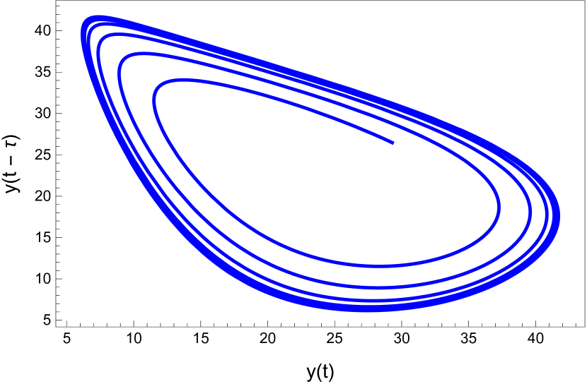
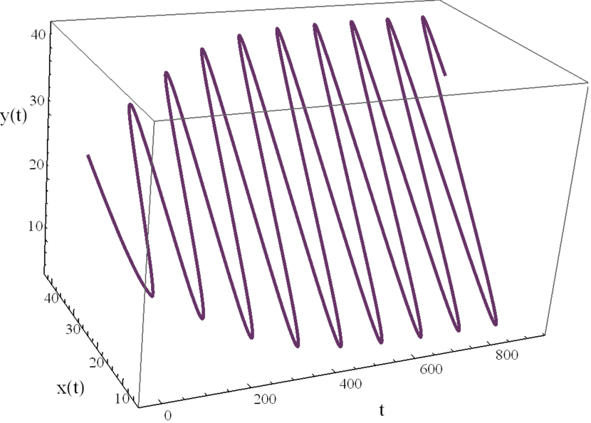
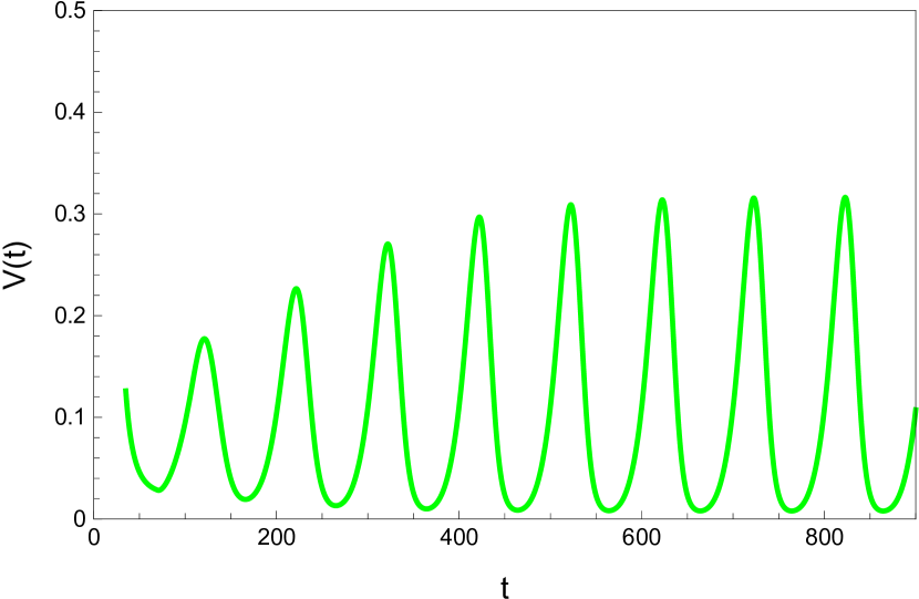
4.2 The dynamic behavior with $\alpha=0.6\textrm{ and }\beta=0.6$

Here we study the dynamic behavior of system (5) by changing the time delay $\tau$ with $\alpha=0.6$ and $\beta=0.6.$ Again the simulations have initial conditions of $x(t)=35.5$ and $y(t)=26.5.$ This has a unique positive equilibrium at $(x_{*},y_{*})=(23.4108,23.4108)$ as listed in 5. We observe that the equilibrium is stable for $\tau<24.9072$ and unstable for $\tau>24.9072.$ At a Hopf bifurcation, no new equilibrium arise. A periodic solution emerges at the equilibrium point as $\tau$ passes through the bifurcation value.

5 Conclusion

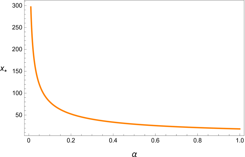
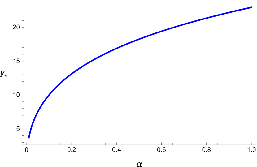
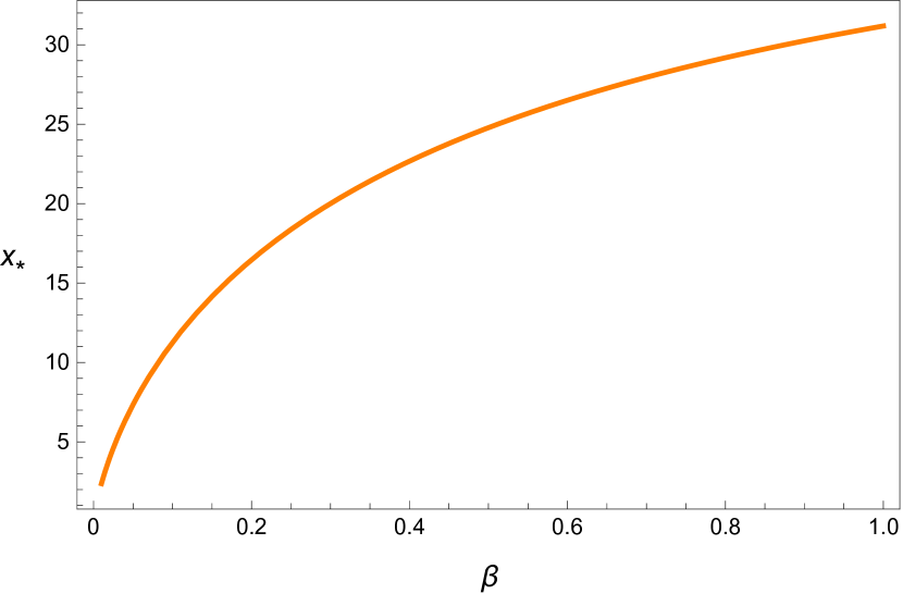
We applied nonlinear delay differential equation in modeling the human respiratory system. The two state model which describes the balance equation for carbon dioxide and oxygen was studied. This model has three parameters $\alpha,$ $\beta$ and $\tau.$ The parameters $\alpha$ and $\beta$ affect the unique positive equilibrium $(x_{*},y_{*})$ of the model (see Figures 2 and 3) and the time delay $\tau$ affects the stability of the system (see Figures 4, 5, 6 and 8.) The critical curves (Equation 25) were used in studying the stability of our model. The three dimensional stability chart is constructed as shown in Figure 7. There is a region enclosed by $\tau=0$ and the curve $\tau=\tau_{1}(0)$ in the $(\tau,\alpha)$ and $(\tau,\beta)$ plane where the equilibrium $(x_{*},y_{*})$ is stable. We have derived analytical expression for equilibrium point and critical delay as a function of $\alpha$ and $\beta$ and we list some of these numerical values in Table 5. These values are also verified by plotting bifurcation diagrams. By picking the delay $\tau$ as the bifurcation parameter, the stability of the positive equilibrium $E_{*}(x_{*},y_{*})$ and the existence of Hopf bifurcation are derived. The equilibrium is asymptotically stable for $0\leq\tau\leq\tau_{*}$ , unstable for $\tau>\tau_{*}.$ The system shows a supercritical Hopf bifurcation giving rise to stable periodic oscillations. These periodic oscillations may be related to the medical condition we refer as periodic breathing. It is to be noted that the delay parameter has effect on the stability but not on the equilibrium state. Additionally, the explicit derivation of the direction of Hopf bifurcation and the stability of the bifurcation periodic solutions are determined with the help of normal form theory and center manifold theorem to delay differential equations.

Finally, some numerical example and simulations are carried out to confirm the analytical findings. The numerical simulations verify the theoretical results.

References

Altevogt et al. [2006] Altevogt, B. M., H. R. Colten, et al. (2006). Sleep disorders and sleep deprivation: an unmet public health problem.
Bairagi and Jana [2011] Bairagi, N. and D. Jana (2011). On the stability and hopf bifurcation of a delay-induced predator–prey system with habitat complexity. Applied Mathematical Modelling 35(7), 3255–3267.
Batzel et al. [2007] Batzel, J. J., F. Kappel, D. Schneditz, and H. T. Tran (2007). Cardiovascular and respiratory systems: modeling, analysis, and control. SIAM.
Batzel and Tran [2000] Batzel, J. J. and H. T. Tran (2000). Stability of the human respiratory control system i. analysis of a two-dimensional delay state-space model. Journal of mathematical biology 41(1), 45–79.
Bélair and Campbell [1994] Bélair, J. and S. A. Campbell (1994). Stability and bifurcations of equilibria in a multiple-delayed differential equation. SIAM Journal on Applied Mathematics 54(5), 1402–1424.
Berry et al. [2012] Berry, R. B., R. Budhiraja, D. J. Gottlieb, D. Gozal, C. Iber, V. K. Kapur, C. L. Marcus, R. Mehra, S. Parthasarathy, S. F. Quan, et al. (2012). Rules for scoring respiratory events in sleep: update of the 2007 aasm manual for the scoring of sleep and associated events: deliberations of the sleep apnea definitions task force of the american academy of sleep medicine. Journal of clinical sleep medicine 8(5), 597–619.
Bhalekar [2016] Bhalekar, S. (2016). Stability analysis of uçar prototype delayed system. Signal, Image and Video Processing 10(4), 777–781.
Bi and Ruan [2013] Bi, P. and S. Ruan (2013). Bifurcations in delay differential equations and applications to tumor and immune system interaction models. SIAM Journal on Applied Dynamical Systems 12(4), 1847–1888.
Bılazeroğlu et al. [2022] Bılazeroğlu, Ş., H. Merdan, and L. Guerrini (2022). Hopf bifurcations of a lengyel-epstein model involving two discrete time delays. Discrete & Continuous Dynamical Systems-S 15(3), 535.
Çelik [2008] Çelik, C. (2008). The stability and hopf bifurcation for a predator–prey system with time delay. Chaos, Solitons & Fractals 37(1), 87–99.
Celik [2015] Celik, C. (2015). Stability and hopf bifurcation in a delayed ratio dependent holling–tanner type model. Applied Mathematics and Computation 255, 228–237.
Cooke and Turi [1994] Cooke, K. L. and J. Turi (1994). Stability, instability in delay equations modeling human respiration. Journal of Mathematical Biology 32(6), 535–543.
Dell’Anna [2020] Dell’Anna, L. (2020). Solvable delay model for epidemic spreading: the case of covid-19 in italy. Scientific Reports 10(1), 1–10.
Du and Wang [2010] Du, L. and M. Wang (2010). Hopf bifurcation analysis in the 1-d lengyel–epstein reaction–diffusion model. Journal of mathematical analysis and applications 366(2), 473–485.
Eckert et al. [2007] Eckert, D. J., A. S. Jordan, P. Merchia, and A. Malhotra (2007). Central sleep apnea: pathophysiology and treatment. Chest 131(2), 595–607.
Epstein and Pojman [1998] Epstein, I. R. and J. A. Pojman (1998). An introduction to nonlinear chemical dynamics: oscillations, waves, patterns, and chaos. Oxford university press.
Ghosh et al. [2021] Ghosh, M., S. Das, and P. Das (2021). Dynamics and control of delayed rumor propagation through social networks. Journal of Applied Mathematics and Computing, 1–30.
Gilsinn [2002] Gilsinn, D. E. (2002). Estimating critical hopf bifurcation parameters for a second-order delay differential equation with application to machine tool chatter. Nonlinear Dynamics 30(2), 103–154.
Guglielmi et al. [2022] Guglielmi, N., E. Iacomini, and A. Viguerie (2022). Delay differential equations for the spatially resolved simulation of epidemics with specific application to covid-19. Mathematical Methods in the Applied Sciences.
Hassard et al. [1981] Hassard, B. D., B. Hassard, N. D. Kazarinoff, Y.-H. Wan, Y. W. Wan, et al. (1981). Theory and applications of Hopf bifurcation, Volume 41. CUP Archive.
Javaheri et al. [1998] Javaheri, S., T. Parker, J. Liming, W. Corbett, H. Nishiyama, L. Wexler, and G. Roselle (1998). Sleep apnea in 81 ambulatory male patients with stable heart failure: types and their prevalences, consequences, and presentations. Circulation 97(21), 2154–2159.
Khellaf and Hamri [2010] Khellaf, W. and N. Hamri (2010). Boundedness and global stability for a predator-prey system with the beddington-deangelis functional response. Differential Equations and Nonlinear Mechanics 2010.
Khoo et al. [1982] Khoo, M., R. E. Kronauer, K. P. Strohl, and A. S. Slutsky (1982). Factors inducing periodic breathing in humans: a general model. Journal of applied physiology 53(3), 644–659.
Kollar and Turi [2005] Kollar, L. E. and J. Turi (2005). Numerical stability analysis in respiratory control system models. In Electronic Journal of Differential Equations: Proceedings of 2004 Conference on Differential Equations and Applications in Mathematical Biology, Volume 12, pp. 65–78. Texas State University.
Kumar et al. [2020] Kumar, R., A. K. Sharma, and K. Agnihotri (2020). Hopf bifurcation analysis in a multiple delayed innovation diffusion model with Holling II functional response. Mathematical Methods in the Applied Sciences 43(4), 2056–2075.
Lakshmanan and Senthilkumar [2011] Lakshmanan, M. and D. V. Senthilkumar (2011). Dynamics of nonlinear time-delay systems. Springer Science & Business Media.
Lanfranchi et al. [1999] Lanfranchi, P. A., A. Braghiroli, E. Bosimini, G. Mazzuero, R. Colombo, C. F. Donner, and P. Giannuzzi (1999). Prognostic value of nocturnal cheyne-stokes respiration in chronic heart failure. Circulation 99(11), 1435–1440.
Leung and Douglas Bradley [2001] Leung, R. S. and T. Douglas Bradley (2001). Sleep apnea and cardiovascular disease. American journal of respiratory and critical care medicine 164(12), 2147–2165.
Li et al. [2004] Li, C., X. Liao, and J. Yu (2004). Hopf bifurcation in a prototype delayed system. Chaos, Solitons & Fractals 19(4), 779–787.
Li and Zhang [2021] Li, L. and Y. Zhang (2021). Dynamic Analysis and Hopf Bifurcation of a Lengyel–Epstein System with Two Delays. Journal of Mathematics 2021.
Li et al. [2019] Li, T., Y. Wang, and X. Zhou (2019). Bifurcation analysis of a first time-delay chaotic system. Advances in Difference Equations 2019(1), 1–18.
Li et al. [1999] Li, X., S. Ruan, and J. Wei (1999). Stability and bifurcation in delay–differential equations with two delays. Journal of Mathematical Analysis and Applications 236(2), 254–280.
Liu et al. [2020] Liu, Z., P. Magal, O. Seydi, and G. Webb (2020). A covid-19 epidemic model with latency period. Infectious Disease Modelling 5, 323–337.
Macke and Glass [1977] Macke, M. and L. Glass (1977). Oscillation and chaos in physiological control system. Science 197, 287–289.
Menéndez [2020] Menéndez, J. (2020). Elementary time-delay dynamics of covid-19 disease. medRxiv.
Murray [2002] Murray, J. D. (2002). Mathematical biology: I. An introduction. Springer.
Paul and Lorin [2021] Paul, S. and E. Lorin (2021). Distribution of incubation periods of covid-19 in the canadian context. Scientific Reports 11(1), 1–9.
Rihan and Alsakaji [2021] Rihan, F. and H. Alsakaji (2021). Dynamics of a stochastic delay differential model for covid-19 infection with asymptomatic infected and interacting people: Case study in the uae. Results in Physics 28, 104658.
Roose and Szalai [2007] Roose, D. and R. Szalai (2007). Continuation and bifurcation analysis of delay differential equations. In Numerical continuation methods for dynamical systems, pp. 359–399. Springer.
Shayak et al. [2020] Shayak, B., M. M. Sharma, R. H. Rand, A. Singh, and A. Misra (2020). A delay differential equation model for the spread of covid-19. International Journal of Engineering Research and Applications 10(10/3), 1–13.
Song et al. [2004] Song, Y., M. Han, and Y. Peng (2004). Stability and hopf bifurcations in a competitive lotka–volterra system with two delays. Chaos, Solitons & Fractals 22(5), 1139–1148.
Song and Wei [2005] Song, Y. and J. Wei (2005). Local hopf bifurcation and global periodic solutions in a delayed predator–prey system. Journal of Mathematical Analysis and Applications 301(1), 1–21.
Su et al. [2009] Su, Y., J. Wei, and J. Shi (2009). Hopf bifurcations in a reaction–diffusion population model with delay effect. Journal of Differential Equations 247(4), 1156–1184.
Sun et al. [2007] Sun, C., M. Han, and Y. Lin (2007). Analysis of stability and hopf bifurcation for a delayed logistic equation. Chaos, Solitons & Fractals 31(3), 672–682.
Tang and Zhou [2007] Tang, Y. and L. Zhou (2007). Stability switch and hopf bifurcation for a diffusive prey–predator system with delay. Journal of Mathematical Analysis and Applications 334(2), 1290–1307.
Uçar [2002] Uçar, A. (2002). A prototype model for chaos studies. International journal of engineering science 40(3), 251–258.
Wang et al. [2012] Wang, X., H. Liu, and C. Xu (2012). Hopf bifurcations in a predator-prey system of population allelopathy with a discrete delay and a distributed delay. Nonlinear Dynamics 69(4), 2155–2167.
Wei [2007] Wei, J. (2007). Bifurcation analysis in a scalar delay differential equation. Nonlinearity 20(11), 2483.
[49] Wolfram Research, I. Mathematica, Version 12.1. Champaign, IL, 2020.
Yafia [2007] Yafia, R. (2007). Hopf bifurcation in differential equations with delay for tumor–immune system competition model. SIAM Journal on Applied Mathematics 67(6), 1693–1703.
Yan and Li [2006] Yan, X.-P. and W.-T. Li (2006). Hopf bifurcation and global periodic solutions in a delayed predator–prey system. Applied Mathematics and Computation 177(1), 427–445.
Zhang et al. [2013] Zhang, G., Y. Shen, and B. Chen (2013). Hopf bifurcation of a predator–prey system with predator harvesting and two delays. Nonlinear Dynamics 73(4), 2119–2131.
Zhou et al. [2012] Zhou, X., X. Chen, and Y. Song (2012). Hopf bifurcation of a differential-algebraic bioeconomic model with time delay. Journal of Applied Mathematics 2012.

$\displaystyle 1$	$\displaystyle=\left<q^{*}(s),q(\vartheta)\right>$	(51)
	$\displaystyle=\bar{q}^{}(0)q(0)-\int_{-1}^{0}\int_{\xi=0}^{\vartheta}\bar{q}^{}(\xi-\vartheta)d\eta(\vartheta)q(\xi)d\xi$
	$\displaystyle=\bar{D}(1,\bar{c}^{})(1,c)^{T}-\int_{-1}^{0}\int_{\xi=0}^{\vartheta}\bar{D}(1,\bar{c}^{})e^{-i\omega_{}\tau_{}(\xi-\vartheta)}d\eta(\vartheta)(1,c)^{T}e^{i\omega_{}\tau_{}\xi}d\xi$
	$\displaystyle=\bar{D}(1,\bar{c}^{})(1,c)^{T}-\bar{D}(1,\bar{c}^{})\int_{-1}^{0}\int_{\xi=0}^{\vartheta}d\eta(\vartheta)(1,c)^{T}e^{i\omega_{}\tau_{}\vartheta}d\xi$
	$\displaystyle=\bar{D}(1,\bar{c}^{})(1,c)^{T}-\bar{D}(1,\bar{c}^{})\int_{-1}^{0}\vartheta e^{i\omega_{}\tau_{}\vartheta}d\eta(\vartheta)(1,c)^{T}$
	$\displaystyle=\bar{D}\left\{1+c\bar{c}^{}+\bar{c}^{}\tau_{}\left(-\frac{7e^{\frac{\gamma}{20}-5}(20\alpha+\beta c\gamma)\left(\beta c^{}y_{}+\alpha x_{}\right)}{1000\alpha}\right)e^{-i\omega_{}\tau_{}}\right\}$

$\displaystyle-i\omega_{}\tau_{}\left<q^{*},\bar{q}\right>$	$\displaystyle=\left<q^{*},A\bar{q}\right>$	(53)
	$\displaystyle=\left<A^{}q^{},\bar{q}\right>$
	$\displaystyle=\left<A^{}q^{},\bar{q}\right>$
	$\displaystyle=i\omega_{}\tau_{}\left<q^{*},\bar{q}\right>$

$\displaystyle\dot{z}(t)$	$\displaystyle=\left<q^{},\dot{x}_{t}\right>=\left<q^{},A(0)\dot{x}_{t}+R(0)x_{t}\right>$	(54)
	$\displaystyle=\left<q^{},A(0)\dot{x}_{t}\right>+\left<q^{},R(0)x_{t}\right>$
	$\displaystyle=\left<A^{}(0)q^{},\dot{x}_{t}\right>+\bar{q}^{*}(0)f_{0}(z,\bar{z})$
	$\displaystyle=i\omega_{}\tau_{}z+g(z,\bar{z})$

Stability and Hopf bifurcation analysis of a two state delay differential equation modeling the human respiratory system

Abstract

1 Introduction

1.1 Components of the Model

1.1.1 Central chemoreceptors

1.1.2 Peripheral chemoreceptors

1.1.3 Ventilation function

1.2 Model equation

2 Stability and Hopf Bifurcation

2.1 Equilibrium point

Lemma 2.1.

Proof.

2.2 Stability of the Equilibrium point

Theorem 2.2.

2.3 Critical Delay and Bifurcation

2.4 Bifurcation Diagram

3 Direction and Stability of the Hopf Bifurcation

4 Numerical Simulations

4.1 The dynamic behavior with α=0.5​ and ​β=0.8\alpha=0.5\textrm{ and }\beta=0.8

4.2 The dynamic behavior with α=0.6​ and ​β=0.6\alpha=0.6\textrm{ and }\beta=0.6

5 Conclusion

References

4.1 The dynamic behavior with $\alpha=0.5\textrm{ and }\beta=0.8$

4.2 The dynamic behavior with $\alpha=0.6\textrm{ and }\beta=0.6$