Stability of energy landscape for Ising models
Abstract
In this paper, we explore the stability of the energy landscape of an Ising Hamiltonian when subjected to two kinds of perturbations: a perturbation on the coupling coefficients and external fields, and a perturbation on the underlying graph structure. We give sufficient conditions so that the ground states of a given Hamiltonian are stable under perturbations of the first kind in terms of order preservation. Here by order preservation we mean that the ordering of energy corresponding to two spin configurations in a perturbed Hamiltonian will be preserved in the original Hamiltonian up to a given error margin. We also estimate the probability that the energy gap between ground states for the original Hamiltonian and the perturbed Hamiltonian is bounded by a given error margin when the coupling coefficients and local external magnetic fields of the original Hamiltonian are i.i.d. Gaussian random variables. In the end we show a concrete example of a system which is stable under perturbations of the second kind.
1 Introduction
Finding optimal solutions for combinatorial optimization problems, some of which are known to be NP-hard, is a very important problem. Among many possible approaches to such problems, the application of Ising models to solve real social problems has been getting attention due to its versatility (see [1]). More precisely, a given social combinatorial optimization problem can be mapped into a Hamiltonian on a graph , whose expression is given by
for every Ising spin configuration , where are coupling coefficients and are local magnetic fields. In that approach, an optimal solution for the intended combinatorial problem corresponds to a ground state (or global minimum) of , that is, . There are some well-known methods that can be applied to obtain a ground state. Implementing a Markov chain Monte Carlo (such as Glauber dynamics and stochastic cellular automata) is known as a way to find an approximation for the Gibbs distribution whose highest peaks correspond to the ground states of . We refer for details to [2, 3, 4, 5] and also [6].
However, as long as we use Ising machines or any computer to perform numerical simulations to find a ground state, we cannot avoid the error occurring due to the analog nature or the difficulty of representing real numbers (see [7]). Because of these reasons, we should incorporate the error coming from the coupling coefficients and local magnetic fields by introducing a perturbed Hamiltonian. Hence, our original Hamiltonian will be perturbed, originating a perturbed Hamiltonian whose coupling coefficients and local magnetic fields have a maximal error . Then, the following natural questions arise:
-
(1)
For any pair of configurations which are ordered in terms of energy with respect to the perturbed Hamiltonian , is that ordering preserved in the original Hamiltonian , up to a given error margin?
-
(2)
Given a Hamiltonian with coupling coefficients and local magnetic fields distributed as i.i.d. Gaussian random variables, what is the probability that the energy gap in between two ground states respectively for and the corresponding perturbed Hamiltonian is sufficiently small?
In addition to the above questions (1) and (2), the following problem is also important when using Ising machines and computers. It may be somewhat a waste of resources taking all coupling coefficients and local magnetic fields into account. It may be useful to “eliminate” vertices of a given graph whose contribution to the total energy is relatively small, in order to save memories of computers. Hence, we also have the following natural question:
-
(3)
Can we find a subset of a given graph such that for an arbitrary choice of configuration outside of that region, the energy variation can be controlled?
In this paper, we investigate the stability of energy landscape of a given Hamiltonian under perturbations from the view point of order preservation, aiming at answering the questions we addressed above. Thanks to the order preservation property, we can obtain better estimates for the success probability of finding a ground state compared to the result given in [7].
This paper is organized as follows. In Section 2, we provide a precise formulation for the questions we just posed and raise them again. In Section 3, we answer the questions (1’) and (2’) from Section 2. In Section 4, we provide an example together with a sufficient condition that guarantees a positive answer for question (3’).
2 Setting and the main questions
In this section, we introduce some necessary definitions and terminologies for discussing the stability of energy landscape. Further we also introduce the notion of order preservation for a perturbed system, which plays a central role in this paper. Here, order preservation means, roughly speaking, if we take a ground state for a perturbed Hamiltonian (implemented by a device) then it should be close to the ground state for an original Hamiltonian (intended mathematical problem) in energy, up to a given error margin.
Let us begin by introducing the precise setting. Let be a finite simple graph with the vertex set and the edge set . The so-called original Hamiltonian with coupling coefficients and external magnetic fields on is defined by
| (2.1) |
for each . Such a function can be regarded as a cost function of an intended problem. Given , we denote by the perturbed Hamiltonian with the coupling coefficients and external fields , i.e.,
| (2.2) |
where the ’s and ’s satisfy the bounds and . This perturbation will be often interpreted as a round-off in the following way. Let and be the binary expansions of the fractional parts of and , i.e.,
| (2.3) |
where and for . If we set and in the equation (2.2), then the error can be taken as . It means that the perturbed Hamiltonian is obtained by rounding off the given parameters ’s and ’s uniformly from the -th digit of their binary expansions.
The main purpose of this paper is to clarify the stability of the ground states for a given Hamiltonian under a perturbation in terms of order preservation. In this paper, we will answer the following questions:
-
(1’)
Find a corresponding to a given , so that, for any pair that satisfies , the ordering is preserved in up to the error margin , i.e.,
(2.4) Here, is the total margin of the original Hamiltonian.
-
(2’)
Let be a probability space and let and be mutually independent standard Gaussian random variables on this probability space. Estimate the probability that the energy gap in between ground states for and , say and , respectively, is controled by the given error margin, explicitly,
(2.5)
A different aspect of stability of a given system is to find a nontrivial subsystem so that the energy gap between any two spin configurations whose spins restricted to the subgraph coincide is bounded above by a given error margin. Also, at the same time, we require that the number of vertices that can be disregarded is at least of order , where and , so that such a number can go to infinity as . In the later part of this paper, we answer the following question for a particular case:
-
(3’)
Let , and let and be mutually independent standard Gaussian random variables. Find a subset for a given and such that
is close to , where is the spin configuration restricted to and is the restriction of the spin configuration to .
Questions (1’), (2’) and (3’) above correspond to questions (1), (2) and (3) from Section 1, respectively. In Section 3, we investigate the first two questions above, where for the second one we adopt two different approaches. We obtain answers for question (2’) by means of a method involving the -distance and a graph’s structure approach, and we compare these two methods for three different graphs. Specifically, we consider sufficient conditions on the perturbation to satisfy order preservation, and calculate the probability that such a sufficient condition holds. In Section 4, we obtain an answer for the question (3’) when the graph is a one-dimensional torus without external fields.
3 Stability under a Hamiltonian perturbation
This part is dedicated to provide solutions for questions (1’) and (2’) just posed in the end of the previous section. Before we proceed to the next sections, let us introduce the quantity defined by
| (3.1) |
which is defined whenever a Hamiltonian is given. Moreover, if is a finite simple graph, then we define by
| (3.2) |
Keeping in mind the mathematical setting introduced in the beginning of Section 2, let us start by showing that the order preservation property holds, that is, let us first answer the question (1’), which consists in finding a corresponding to a given such that implies ; and later on, assuming some randomness on the spin-spin couplings and external fields, we adopt two different approaches to answer question (2’) and estimate the probability that the condition is satisfied.
In order to solve the second problem, we will adopt two distinct approaches: a method that relies on uniform estimates and a method where combinatorial estimates are considered instead, which will be presented in Sections 3.2 and 3.3, respectively. In the last part of this section, we compare these two methods and conclude that depending on the underlying graph structure of the problem, one of them will give us a better lower bound for the probability from equation (2.5).
3.1 Order preservation of energy
The answer for question (1’) from Section 2 is provided by Theorem 3.2, however, let us show first a preliminary result.
In [5], we have already established lower bounds for the total margin of the Hamiltonian , but for the reader’s convenience we include its proof in the present paper.
Lemma 3.1 (See [5]).
Let us consider a finite simple graph and a Hamiltonian written in the form
for each . Then, we have
Proof.
For any probability measure on the configuration space , we have
where stands for the expectation with respect to the probability measure . If is particularly chosen as the uniform distribution on , then we have
and
Therefore, . ∎
In order to prove the next result, it is convenient to consider the following notation introduced by [7]. For any Ising spin configurations and , we consider the sets and defined by
and
where the products and are called the spin overlap and the link overlap, respectively.
Theorem 3.2.
Given and configurations and , if the condition
is satisfied, then implies .
Proof.
If we suppose that , then, we have
Since , , , and , then, by our assumption, we obtain
Therefore, the conclusion of this theorem follows. ∎
3.2 Stability of ground states: first approach
In the previous subsection, we did not assume any randomness on the spin-spin couplings ’s and local external fields ’s. In this subsection, let us consider the same setting as stated in question (2’) from Section 2. Precisely speaking, we assume that and are mutually independent random variables distributed according to a standard Gaussian distribution.
Under such assumptions, let us estimate the probability that the inequality holds, where is a given positive constant, by using a method that relies on uniform bounds with respect to certain spin configurations. In the following lemma, we provide an upper bound for the difference .
Lemma 3.3.
Given , if and are ground states for and , respectively, then, we have
| (3.3) |
Proof.
It follows from the definition of a ground state that , then
where stands for the uniform norm, as usual. Furthermore, for any spin configuration , we have
Then, , therefore, we conclude the proof. ∎
By the lemma above , it follows that
and by using the fact that (see Lemma 3.1), we conclude that
| (3.4) |
Finally, we have the following estimation for the probability that holds, which consists of one of the answers for the question (2’).
Theorem 3.4.
Let and be mutually independent standard Gaussian random variables. It follows that
| (3.5) |
where is the distribution function of the chi-square distribution with degrees of freedom, that is,
for , and for .
Proof.
It follows from the above discussion that we have
Since and are mutually independent random variables distributed according to a standard Gaussian distribution, then the random variable is distributed as the chi-square distribution with degrees of freedom. Therefore,
Thus, we obtain the lower bound of the target probability. ∎
3.3 Stability of ground states: second approach
Before we proceed, let us point out the fundamental difference between the uniform approach and the current approach to solve question (2’). Note that, if we use the same computations as considered in the proof of Theorem 3.2 in the particular case where and and use the fact that , then it follows that
| (3.6) |
Recall that the proof of Theorem 3.4 fundamentally relied on the fact that, by using the -distance estimates, the left-hand side of equation (3.6) could be bounded above by . Note that the right-hand side of equation (3.6) is also bounded above by , therefore, let us explore the geometry of the underlying graph in order to see whether it is possible to obtain better bounds.
The value of depends on the underlying graph structure and the relationship between the ground states and . Therefore, we should check the value of for the intended problem. In general, we look for a uniform estimation for the value of for any and since the ground states and in practice are unknown. First, let us show the following lemma.
Lemma 3.5.
For any two configurations and , we have
where stands for the maximum degree of .
Proof.
Let us assume that , for some such that . Then, let us enumerate as , where for each . Moreover, we have , and therefore we can write , where for each . By the definition of , we have for every and for all . If for distinct and in , then
Thus, . In a similar way, we conclude that in case for distinct and in , it follows that . If for some and some , then
Hence, . It follows that
Therefore, we have
∎
Proposition 3.6.
For any graph , let and be two spin configurations. Then, we have
| (3.7) |
Proof.
Thus, we have the following theorem which is another answer for the question (2’) (see Theorem 3.4 for an alternative approach to the question (2’)).
Theorem 3.7.
Let and be mutually independent standard Gaussian random variables. Then, we have
| (3.8) |
3.4 Comparison between approaches
In the rest of this section, we compare the methods presented in Sections 3.2 and 3.3 passing through several examples to which we apply Proposition 3.6.
The first example is the case where we consider complete graphs including the SK model. If we consider complete graphs, then Theorem 3.7 provides us with better results if compared to Theorem 3.4.
Example 3.8.
If is a complete graph (that is, all vertices are connected to each other) with vertices, then we have
On the other hand, the value of will be given by
Therefore,
Hence the uniform upper bound for we obtained in Proposition 3.6 is always better than . Furthermore, we can calculate the explicit value of when is a complete graph. From the proof of Lemma 3.5, by assuming that is a complete graph, we can say that . Therefore,
and the proof of Theorem 3.7 implies
The following example considers King’s graphs and Theorem 3.7 works better than Theorem 3.4 as well as the above example.
Example 3.9.
Let be an King’s graph. The King’s graph can be visualized as an chessboard where each of its squares corresponds to a vertex of the graph, and each edge represents a legal move of a king in a chess game. In that way, the inner vertices of the graph have neighbors each, while the vertices in the corners have neighbors each, and each of the remaining vertices on the sides of the graph has neighbors. For an King’s graph, we have
since . Moreover, we have
If and are sufficiently large, then we have
In the following example, differently from the previous ones, we can see that the estimate provided by Theorem 3.4 suits better than that of Theorem 3.7.
Example 3.10.
If is a star graph with degree , that is, consists of one vertex placed in the center and other vertices connected only with the center, then
Furthermore, we have
Therefore, we obtain
According to the above examples, we conclude that it is not always possible to guarantee that the uniform upper bound of provided by Proposition 3.6 works better than . Thus, we may have to consider such bounds separately when considering different graphs in order to obtain an optimal estimate for the probability that inequality holds.
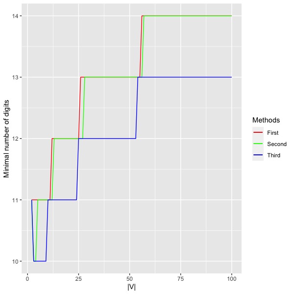
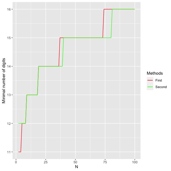
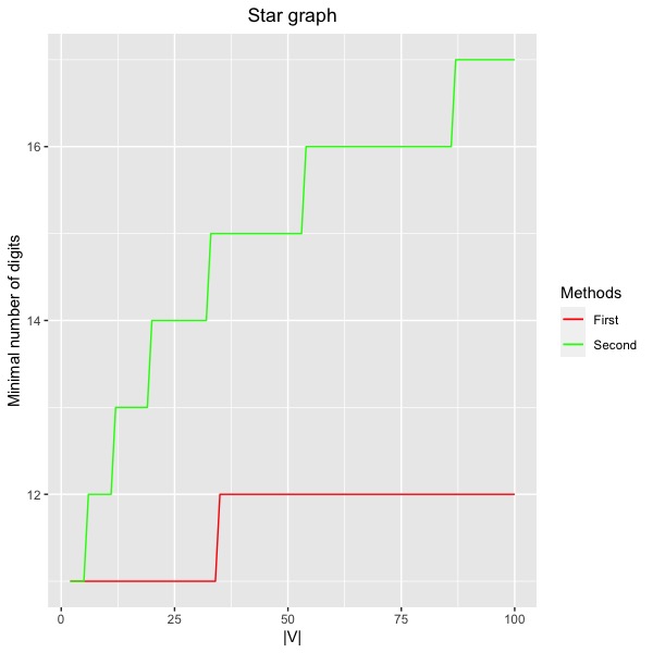
Let us consider again the problem of stability where we take into account only a finite number of terms in the binary expansions of the parameters and as we illustrated in the beginning of Section 2. In Figure 1, corresponding to the sizes of different graphs, we show the minimum number of digits necessary to be considered in the binary expansions of such parameters such that with probability at least the difference represents a value smaller than of . On each plot we compare the different methods developed in this paper, where the first method corresponds to the estimate from Theorem 3.4 and the second method corresponds to the estimate from Theorem 3.7. In Figure 1(a), we also included a third estimate from Example 3.8 which is sharper and gives us better results when compared to the other methods. As we expected, the second method provides us with better results when compared to the first one for complete graphs and for King’s graphs when is sufficiently large. On the other hand, for star graphs the first method is more appropriate, moreover, a certain discrepancy of performance is easily observed.
4 Stability under a perturbed graph
In this section, we consider the stability of energy landscape when a given spin system defined on a graph is compressed into a smaller subsystem. Differently from the previous sections, we fix a given Hamiltonian and we assume a sufficient condition that guarantees the existence of a nontrivial subset of the entire vertex set outside of which we can randomly assign any spin configuration and the energy of the system is kept under control up to a certain error margin.
Let be a finite simple graph, and let be the Hamiltonian on given by
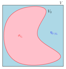
for every configuration , where is a collection of mutually independent standard Gaussian random variables. What we would like to show is that we can compress the whole system into a nontrivial subsystem so that the energy landscape of such subsystem is close to the original one up to a given error margin. More precisely, our goal is to find a class of examples for which given a positive constant , there is a positive such that the subsystem of , defined from the relation
is non-trivial, has size comparable to the size of , and satisfies
| (4.1) |
with high probability, see Figure 2.
4.1 One-dimensional discrete torus
Let us solve the problem stated above in the particular case where the graph is a one-dimensional discrete torus.
Theorem 4.1.
Let be a one-dimensional discrete torus with vertices, that is, and . Given , let be a positive number such that . Then, if is a subset of the event , it follows that
| (4.2) |
holds for each . In particular, given constants and , we have
| (4.3) |
for sufficiently large, where
| (4.4) |
Before we follow to the proof of the result above, let us clarify the theorem by providing the reader with some practical results. Let us consider the particular case where and . Corresponding to different values of and , we obtain lower bounds for the probability that the size of is at least and condition (4.1) holds, see the table below.
Let us observe that for any pair of spin configurations, we have
In particular, if is the one-dimensional torus as in Theorem 4.1, it follows that
| (4.5) |
Now, let us prepare two lemmas in order to prove Theorem 4.1.
Lemma 4.2.
For , we have
| (4.6) |
hence, with probability 1,
Proof.
Without loss of generality, we assume . Let us fix . Then, depending on the sign of , we can determine to minimize (or maximize) . We continue this procedure up to and we have
(the additional terms exist if frustration exist at and ). Hence the inequality of the lemma is proven.
To show the last statement, we divide all terms by and use the law of large numbers for the folded normal distribution. ∎
Lemma 4.3.
If we assume , then it follows that
and
Proof.
For each , let us define a random variable by letting
Then, by the definition of , the condition is equivalent to . Therefore, the expected value of the size of will be given by
Furthermore, we write
Here, the random variables and are not mutually independent but we have
Thus, it follows that the identity
holds, and we complete the proof. ∎
Proof of Theorem 4.1.
Let us start by splitting the probability in the left-hand side of equation (4.2) as
where is the event given by
| (4.7) |
From equation (4.5), Lemma 4.2, and the fact that, under condition (subset of ), , it follows that the conditional probability above satisfies
then
| (4.8) |
The rest of the proof consists of estimating the probability of the event . Let us write
| (4.9) |
It follows from Chebyshev’s inequality that
| (4.10) |
where is the variance of the folded Gaussian random variable which is equal to . By using equations (4.8), (4.9) and (4.10), equation (4.2) follows.
4.2 Generalizations
The most natural step in further investigations is to extend the results obtained in Section 4.1 to the case where we include i.i.d. standard Gaussian external fields, and also extend such results to a larger class of examples such as to a -dimensional torus or even to finite graphs with bounded degree. Note that, by assuming the absence of external fields, in the same way as we obtained inequality (4.5), one can show that
| (4.12) |
holds for any graph. So, analogously as in the one-dimensional torus case, it is expected that if we find a lower bound for , as we did in Lemma 4.2, which is comparable to the right-hand side of equation (4.12), then we may derive an extension of our results for a larger class of graphs. Some numerical results suggest that, for an Ising spin system in a -dimensional torus with i.i.d. standard Gaussian spin-spin couplings and without external fields, is still of order , but it still lacks a rigorous proof of that observation due to the difficulty of dealing with frustrated configurations in a higher dimensional torus.
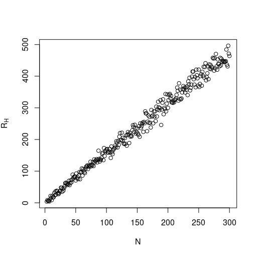
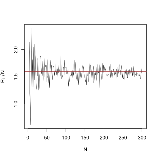
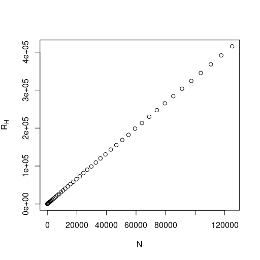
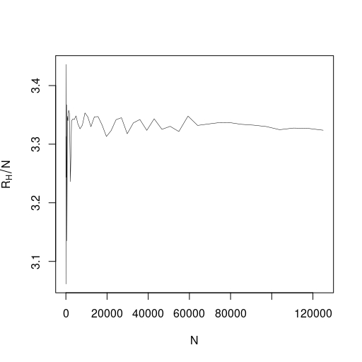
The simulations presented in this section were performed by using a modified version of the stochastic cellular automata algorithm studied in [5, 6] to estimate the maximum and minimum value of the Hamiltonian in order to find an approximation of corresponding to different values of . Note that, in such plots, each dot represents the value of (resp. ) corresponding to a torus with vertices for a realization of the random values of spin-spin couplings (i.i.d. standard Gaussian random variables). In the one-dimensional case (see Figure 3), we see that the value of approximates the value , as expected due to Lemma 4.2.
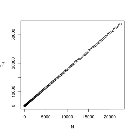
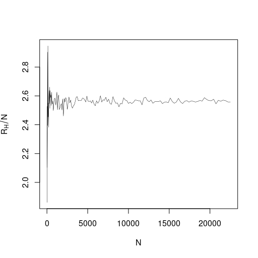
Now, for the two and three dimensional cases (see Figure 4), when we consider larger values of , the value of seems to approximate the values and , respectively. Note that such simulated values represent lower bounds for the real value of the limit as approaches infinity, so the true limits are still unknown. Furthermore, we conjecture that such limit exists in any dimension and the random variable converges almost surely due to the fact that, in higher dimension, its simulated values seem to fluctuate less around an asymptotic limit as compared to the one-dimensional case.
It is straightforward to show that, for the -dimensional torus, we have
where stands for the -th canonical vector of the -dimensional Euclidean space, then
| (4.13) |
Moreover, it follows from the fact that (see Lemma 3.1) and the Cauchy–Schwarz inequality that
| (4.14) |
Therefore, we see that there is still room for improvement and the need of rigorous proofs about the existence and determination of the limit , originating a mathematical problem which is interesting by itself.
Acknowledgment
This work was supported by JST CREST Grant Number JP22180021, Japan. We would like to thank Takashi Takemoto and Normann Mertig of Hitachi, Ltd., for providing us with a stimulating platform for the weekly meeting at Global Research Center for Food & Medical Innovation (FMI) of Hokkaido University. We would also like to thank Hiroshi Teramoto of Kansai University, as well as Masamitsu Aoki, Yoshinori Kamijima, Katsuhiro Kamakura, Suguru Ishibashi and Takuka Saito of Mathematics Department, for valuable comments and encouragement at the aforementioned meetings at FMI.
References
- [1] A. Lucas, Ising formulations of many NP problems. Front. Phys. 12 (2014): https://doi.org/10.3389/fphy.2014.00005.
- [2] P. Dai Pra, B. Scoppola, E. Scoppola, Sampling from a Gibbs measure with pair interaction by means of PCA, J. Stat. Phys. 149 (2012): 722-737.
- [3] B. Hajek, Cooling schedules for optimal annealing. Math. Oper. Res. 13 (2), (1988): 311-329.
- [4] M. C. Robini, Theoretically ground acceleration techniques for simulated annealing, Handbook of Optimization (2013).
- [5] S. Handa, K. Kamakura, Y. Kamijima, A. Sakai, Finding optimal solutions by stochastic cellular automata, arXiv:1906.06645.
- [6] B. H. Fukushima-Kimura, S. Handa, K. Kamakura, Y. Kamijima, A. Sakai, Mixing time and simulated annealing for the stochastic cellular automata, arXiv:2007.11287v2.
- [7] T. Albash, V. M. Mayor, I. Hen, Analog Errors in Ising Machines, arXiv:1806.03744.