Stabilizing Dynamical Systems via Policy Gradient Methods
Abstract
Stabilizing an unknown control system is one of the most fundamental problems in control systems engineering. In this paper, we provide a simple, model-free algorithm for stabilizing fully observed dynamical systems. While model-free methods have become increasingly popular in practice due to their simplicity and flexibility, stabilization via direct policy search has received surprisingly little attention. Our algorithm proceeds by solving a series of discounted LQR problems, where the discount factor is gradually increased. We prove that this method efficiently recovers a stabilizing controller for linear systems, and for smooth, nonlinear systems within a neighborhood of their equilibria. Our approach overcomes a significant limitation of prior work, namely the need for a pre-given stabilizing control policy. We empirically evaluate the effectiveness of our approach on common control benchmarks.
1 Introduction
Stabilizing an unknown control system is one of the most fundamental problems in control systems engineering. A wide variety of tasks - from maintaining a dynamical system around a desired equilibrium point, to tracking a reference signal (e.g a pilot’s input to a plane) - can be recast in terms of stability. More generally, synthesizing an initial stabilizing controller is often a necessary first step towards solving more complex tasks, such as adaptive or robust control design (Sontag, 1999, 2009).
In this work, we consider the problem of finding a stabilizing controller for an unknown dynamical system via direct policy search methods. We introduce a simple procedure based off policy gradients which provably stabilizes a dynamical system around an equilibrium point. Our algorithm only requires access to a simulator which can return rollouts of the system under different control policies, and can efficiently stabilize both linear and smooth, nonlinear systems.
Relative to model-based approaches, model-free procedures, such as policy gradients, have two key advantages: they are conceptually simple to implement, and they are easily adaptable; that is, the same method can be applied in a wide variety of domains without much regard to the intricacies of the underlying dynamics. Due to their simplicity and flexibility, direct policy search methods have become increasingly popular amongst practitioners, especially in settings with complex, nonlinear dynamics which may be challenging to model. In particular, they have served as the main workhorse for recent breakthroughs in reinforcement learning and control (Silver et al., 2016; Mnih et al., 2015; Andrychowicz et al., 2020).
Despite their popularity amongst practitioners, model-free approaches for continuous control have only recently started to receive attention from the theory community (Fazel et al., 2018; Kakade et al., 2020; Tu and Recht, 2019). While these analyses have begun to map out the computational and statistical tradeoffs that emerge in choosing between model-based and model-free approaches, they all share a common assumption: that the unknown dynamical system in question is stable, or that an initial stabilizing controller is known. As such, they do not address the perhaps more basic question, how do we arrive at a stabilizing controller in the first place?
1.1 Contributions
We establish a reduction from stabilizing an unknown dynamical system to solving a series of discounted, infinite-horizon LQR problems via policy gradients, for which no knowledge of an initial stable controller is needed. Our approach, which we call discount annealing, gradually increases the discount factor and yields a control policy which is near optimal for the undiscounted LQR objective. To the best of our knowledge, our algorithm is the first model-free procedure shown to provably stabilize unknown dynamical systems, thereby solving an open problem from Fazel et al. (2018).
We begin by studying linear, time-invariant dynamical systems with full state observation and assume access to inexact cost and gradient evaluations of the discounted, infinite-horizon LQR cost of a state-feedback controller . Previous analyses (e.g., (Fazel et al., 2018)) establish how such evaluations can be implemented with access to (finitely many, finite horizon) trajectories sampled from a simulator. We show that our method recovers the controller which is the optimal solution of the undiscounted LQR problem in a bounded number of iterations, up to optimization and simulator error. The stability of the resulting is guaranteed by known stability margin results for LQR. In short, we prove the following guarantee:
Theorem 1 (informal).
For linear systems, discount annealing returns a stabilizing state-feedback controller which is also near-optimal for the LQR problem. It uses at most polynomially many, -inexact gradient and cost evaluations, where the tolerance also depends polynomially on the relevant problem parameters.
Since both the number of queries and error tolerance are polynomial, discount annealing can be efficiently implemented using at most polynomially many samples from a simulator.
Furthermore, our results extend to smooth, nonlinear dynamical systems. Given access to a simulator that can return damped system rollouts, we show that our algorithm finds a controller that attains near-optimal LQR cost for the Jacobian linearization of the nonlinear dynamics at the equilibrium. We then show that this controller stabilizes the nonlinear system within a neighborhood of its equilibrium.
Theorem 2 (informal).
Discount annealing returns a state-feedback controller which is exponentially stabilizing for smooth, nonlinear systems within a neighborhood of their equilibrium, using again only polynomially many samples drawn from a simulator.
In each case, the algorithm returns a near optimal solution to the relevant LQR problem (or local approximation thereof). Hence, the stability properties of are, in theory, no better than those of the optimal LQR controller . Importantly, the latter may have worse stability guarantees than the optimal solution of a corresponding robust control objective (e.g. synthesis). Nevertheless, we focus on the LQR subroutine in the interest of simplicity, clarity, and in order to leverage prior analyses of model-free methods for LQR. Extending our procedure to robust-control objectives is an exciting direction for future work.
Lastly, while our theoretical analysis only guarantees that the resulting controller will be stabilizing within a small neighborhood of the equilibrium, our simulations on nonlinear systems, such as the nonlinear cartpole, illustrate that discount annealing produces controllers that are competitive with established robust control procedures, such as synthesis, without requiring any knowledge of the underlying dynamics.
1.2 Related work
Given its central importance to the field, stabilization of unknown and uncertain dynamical systems has received extensive attention within the controls literature. We review some of the relevant literature and point the reader towards classical texts for a more comprehensive treatment (Sontag, 2009; Sastry and Bodson, 2011; Zhou et al., 1996; Callier and Desoer, 2012; Zhou and Doyle, 1998).
Model-based approaches. Model-based methods construct approximate system models in order to synthesize stabilizing control policies. Traditional analyses consider stabilization of both linear and nonlinear dynamical systems in the asymptotic limit of sufficient data (Sastry and Bodson, 2011; Sastry, 2013). More recent, non-asymptotic studies have focused almost entirely on linear systems, where the controller is generated using data from multiple independent trajectories (Fiechter, 1997; Dean et al., 2019; Faradonbeh et al., 2018a, 2019). Assuming the model is known, stabilizing policies may also be synthesized via convex optimization (Prajna et al., 2004) by combining a ‘dual Lyapunov theorem’ (Rantzer, 2001) with sum-of-squares programming (Parrilo, 2003). Relative to these analysis our focus is on strengthening the theoretical foundations of model-free procedures and establishing rigorous guarantees that policy gradient methods can also be used to generate stabilizing controllers.
Online control. Online control studies the problem of adaptively fine-tuning the performance of an already-stabilizing control policy on a single trajectory (Dean et al., 2018; Faradonbeh et al., 2018b; Cohen et al., 2019; Mania et al., 2019; Simchowitz and Foster, 2020; Hazan et al., 2020; Simchowitz et al., 2020; Kakade et al., 2020). Though early papers in this direction consider systems without pre-given stabilizing controllers (Abbasi-Yadkori and Szepesvári, 2011), their guarantees degrade exponentially in the system dimension (a penalty ultimately shown to be unavoidable by Chen and Hazan (2021)). Rather than fine-tuning an already stabilizing controller, we focus on the more basic problem of finding a controller which is stabilizing in the first place, and allow for the use of multiple independent trajectories.
Model-free approaches. Model-free approaches eschew trying to approximate the underlying dynamics and instead directly search over the space of control policies. The landmark paper of Fazel et al. (2018) proves that, despite the non-convexity of the problem, direct policy search on the infinite-horizon LQR objective efficiently converges to the globally optimal policy, assuming the search is initialized at an already stabilizing controller. Fazel et al. (2018) pose the synthesis of this initial stabilizing controller via policy gradients as an open problem; one that we solve in this work.
Following this result, there have been a large number of works studying policy gradients procedures in continuous control, see for example Feng and Lavaei (2020); Malik et al. (2019); Mohammadi et al. (2020, 2021); Zhang et al. (2021) just to name a few. Relative to our analysis, these papers consider questions of policy finite-tuning, derivative-free methods, and robust (or distributed) control which are important, yet somewhat orthogonal to the stabilization question considered herein. The recent analysis by Lamperski (2020) is perhaps the most closely related piece of prior work. It proposes a model-free, off-policy algorithm for computing a stabilizing controller for deterministic LQR systems. Much like discount annealing, the algorithm also works by alternating between policy optimization (in their case by a closed-form policy improvement step based on the Riccati update) and increasing a damping factor. However, whereas we provide precise finite-time convergence guarantees to a stabilizing controller for both linear and nonlinear systems, the guarantees in Lamperski (2020) are entirely asymptotic and restricted to linear systems. Furthermore, we pay special attention to quantifying the various error tolerances in the gradient and cost queries to ensure that the algorithm can be efficiently implemented in finite samples.
1.3 Background on stability of dynamical systems
Before introducing our results, we first review some of the basic concepts and definitions regarding stability of dynamical systems. In this paper, we study discrete-time, noiseless, time-invariant dynamical systems with states and control inputs . In particular, given an initial state , the dynamics evolves according to where is a state transition map. An equilibrium point of a dynamical system is a state such that . As per convention, we assume that the origin is the desired equilibrium point around which we wish to stabilize the system.
This paper restricts its attention to static state-feedback policies of the form for a fixed matrix . Abusing notation slightly, we conflate the matrix with its induced policy. Our aim is to find a policy which is exponentially stabilizing around the equilbrium point.
Time-invariant, linear systems, where are stabilizable if and only if there exists a such that is a stable matrix (Callier and Desoer, 2012). That is if , where denotes the spectral radius, or the largest eigenvalue magnitude, of a matrix . For general nonlinear systems, our goal is to find controllers which satisfy the following general, quantitative definition of exponential stability (e.g Chapter 5.2 in Sastry (2013)). Throughout, denotes the Euclidean norm.
Definition 1.1.
A controller is -exponentially stable for dynamics if there exist constants such that if inputs are chosen according to , the sequence of states satisfy
| (1.1) |
Likewise, is -exponentially stable on radius if (1.1) holds for all such that .
For linear systems, a controller is stabilizing if and only if it is stable over the entire state space, however, the restriction to stabilization over a particular radius is in general needed for nonlinear systems. Our approach for stabilizing nonlinear systems relies on analyzing their Jacobian linearization about the origin equilibrium. Given a continuously differentiable transition operator , the local dynamics can be approximated by the Jacobian linearization of about the zero equilibrium; that is
| (1.2) |
In particular, for and sufficiently small, , where is a nonlinear remainder from the Taylor expansion of . To ensure stabilization via state-feedback is feasible, we assume throughout our presentation that the linearized dynamics are stabilizable.
2 Stabilizing Linear Dynamical Systems
We now present our main results establishing how our algorithm, discount annealing, provably stabilizes linear dynamical systems via a reduction to direct policy search methods. We begin with the following preliminaries on the Linear Quadratic Regulator (LQR).
Definition 2.1 (LQR Objective).
For a given starting state , we define the LQR problem with discount factor , dynamic matrices , and state feedback controller as,
Here, , , and are positive definite matrices. Slightly overloading notation, we define
to be the same as the problem above, but where the initial state is now drawn from the uniform distribution over the sphere in of radius .111This scaling is chosen so that the initial state distribution has identity covariance, and yields cost equivalent to .
To simplify our presentation, we adopt the shorthand in cases where the system dynamics are understood from context. Furthermore, we assume that is stabilizable and that . It is a well-known fact that achieves the minimum LQR cost over all possible control laws. We begin our analysis with the observation that the discounted LQR problem is equivalent to the undiscounted LQR problem with damped dynamics matrices.222This lemma is folklore within the controls community, see e.g. Lamperski (2020).
Lemma 2.1.
For all controllers such that ,
From this equivalence, it follows from basic facts about LQR that a controller satisfies if and only if is stable. Consequently, for , the zero controller is stabilizing and one can solve the discounted LQR problem via direct policy search initialized at = 0 (Fazel et al., 2018). At this point, one may wonder whether the solution to this highly discounted problem yields a controller which stabilizes the undiscounted system. If this were true, running policy gradients (defined in Eq. 2.1) to convergence, on a single discounted LQR problem, would suffice to find a stabilizing controller.
| (2.1) |
Unfortunately, the following proposition shows that this is not the case.
Proposition 2.2 (Impossibility of Reward Shaping).
Fix . For any positive definite cost matrices and discount factor such that is stable, there exists a matrix such that is controllable (and thus stabilizable), yet the optimal controller on the discounted problem is such that is unstable.
Discount Annealing Initialize: Objective , , , and , For 1. If , run policy gradients once more as in Step 2, break, and return the resulting . 2. Using policy gradients (see Eq. 2.1) initialized at , find such that: (2.2) 3. Update initial controller . 4. Using binary or random search, find a discount factor such that (2.3) 5. Update the discount factor .
We now describe the discount annealing procedure for linear systems (Figure 1), which provably recovers a stabilizing controller . For simplicity, we present the algorithm assuming access to noisy, bounded cost and gradient evaluations which satisfy the following definition. Employing standard arguments from (Fazel et al., 2018; Flaxman et al., 2005), we illustrate how these evaluations can be efficiently implemented using polynomially many samples drawn from a simulator in Appendix C.
Definition 2.2 (Gradient and Cost Queries).
Given an error parameter and a function , returns a vector such that . Similarly, returns a scalar such that .
The procedure leverages the equivalence (Lemma 2.1) between discounted costs and damped dynamics for LQR, and the consequence that the zero controller is stabilizing if we choose sufficiently small. Hence, for this discount factor, we may apply policy gradients initialized at the zero controller in order to recover a controller which is near-optimal for the discounted objective.
Our key insight is that, due to known stability margins for LQR controllers, is stabilizing for the discounted dynamics for some discount factor , where is a small constant that has a uniform lower bound. Therefore, has finite cost on the discounted problem, so that we may again use policy gradients initialized at to compute a near-optimal controller for this larger discount factor. By iterating, we have that and can increase the discount factor up to 1, yielding a near-optimal stabilizing controller for the undiscounted LQR objective.
The rate at which we can increase the discount factors depends on certain properties of the (unknown) dynamical system. Therefore, we opt for binary search to compute the desired in the absence of system knowledge. This yields the following guarantee, which we state in terms of properties of the matrix , the optimal value function for the undiscounted LQR problem, which satisfies (see Appendix A for further details).
Theorem 1 (Linear Systems).
Let . The following statements are true regarding the discount annealing algorithm when run on linear dynamical systems:
-
a)
Discount annealing returns a controller which is -exponentially stable.
-
b)
If , the algorithm is guaranteed to halt whenever is greater than .
Furthermore, at each iteration :
- c)
- c)
We remark that since need only be polynomially small in the relevant problem parameters, each call to and can be carried out using only polynomially many samples from a simulator which returns finite horizon system trajectories under various control policies. We make this claim formal in Appendix C.
Proof.
We prove part of the theorem and defer the proofs of the remaining parts of to Appendix A. Define to be the solution to the discrete-time Lyapunov equation. That is for stable, solves:
| (2.4) |
Using this notation, is the solution to the above Lyapunov equation with . The key step of the proof is Proposition A.4, which uses Lyapunov theory to verify the following: given the current discount factor , an idealized discount factor defined by
satisfies . Since the control cost is non-decreasing in , the binary search update in Step 4 ensures that the actual also satisfies
The following calculation (which uses for ) justifies the second inequality above:
Therefore, . The precise bound follows from taking logs of both sides and using the numerical inequality to simplify the denominator.
∎
3 Stabilizing Nonlinear Dynamical Systems
We now extend the guarantees of the discount annealing algorithm to smooth, nonlinear systems. Whereas our study of linear systems explicitly leveraged the equivalence of discounted costs and damped dynamics, our analysis for nonlinear systems requires access to system rollouts under damped dynamics, since the previous equivalence between discounting and damping breaks down in nonlinear settings.
More specifically, in this section, we assume access to a simulator which given a controller , returns trajectories generated according to for any damping factor , where is the transition operator for the nonlinear system. While such trajectories may be infeasible to generate on a physical system, we believe these are reasonable to consider when dynamics are represented using software simulators, as is often the case in practice (Lewis et al., 2003; Peng et al., 2018).
The discount annealing algorithm for nonlinear systems is almost identical to the algorithm for linear systems. It again works by repeatedly solving a series of quadratic cost objectives on the nonlinear dynamics as defined below, and progressively increasing the damping factor .
Definition 3.1 (Nonlinear Objective).
For a statefeedback controller , damping factor , and an initial state , we define:
| (3.1) | |||
| (3.2) |
Overloading notation as before, we let .
The normalization by above is chosen so that the nonlinear objective coincides with the LQR objective when is in fact linear. Relative to the linear case, the only algorithmic difference for nonlinear systems is that we introduce an extra parameter which determines the radius for the initial state distribution. As established in Theorem 2, this parameter must be chosen small enough to ensure that discount annealing succeeds. Our analysis pertains to dynamics which satisfy the following smoothness definition.
Assumption 1 (Local Smoothness).
The transition map is continuously differentiable. Furthermore, there exist such that for all with ,
For simplicity, we assume and . Using Assumption 1, we can apply Taylor’s theorem to rewrite as its Jacobian linearization around the equilibrium point, plus a nonlinear remainder term.
Lemma 3.1.
If satisfies Assumption 1, then all for which ,
| (3.3) |
where , , and where are the system’s Jacobian linearization matrices defined in Eq. 1.2.
Rather than trying to directly understand the behavior of stabilization procedures on the nonlinear system, the key insight of our nonlinear analysis is that we can reason about the performance of a state-feedback controller on the nonlinear system via its behavior on the system’s Jacobian linearization. In particular, the following lemma establishes how any controller which achieves finite discounted LQR cost for the Jacobian linearization is guaranteed to be exponentially stabilizing on the damped nonlinear system for initial states that are small enough. Throughout the remainder of this section, we define as the LQR objective from Definition 2.1 where .
Lemma 3.2 (Restatement of Lemma B.2).
Suppose that , then is exponentially stable on the damped system over radius .
The second main building block of our nonlinear analysis is the observation that if the dynamics are locally smooth around the equilibrium point, then by Lemma 3.1, decreasing the radius of the initial state distribution reduces the magnitude of the nonlinear remainder term . Hence, the nonlinear system smoothly approximates its Jacobian linearization. More precisely, we establish that the difference in gradients and costs between and decrease linearly with the radius .
Proposition 3.3.
Assume . Then, for defined as in Eq. 2.4:
-
a)
If , then
-
b)
If , then,
Lastly, because policy gradients on linear dynamical systems is robust to inexact gradient queries, we show that for sufficiently small, running policy gradients on converges to a controller which has performance close to the optimal controller for the LQR problem with dynamic matrices . As noted previously, we can then use Lemma 3.2 to translate the performance of the optimal LQR controller for the Jacobian linearization to an exponential stability guarantee for the nonlinear dynamics. Using these insights, we establish the following theorem regarding discount annealing for nonlinear dynamics.
Theorem 2 (Nonlinear Systems).
Let . The following statements are true regarding the discount annealing algorithm for nonlinear dynamical systems when is less than a fixed quantity that is
-
a)
Discount annealing returns a controller which is -exponentially stable over a radius
-
b)
If , the algorithm is guaranteed to halt whenever is greater than .
Furthermore, at each iteration :
-
c)
Policy gradients achieves the guarantee in Eq. 2.2 using only many queries to as long as is less than some fixed polynomial .
- c)
We note that while our theorem only guarantees that the controller is stabilizing around a polynomially small neighborhood of the equilibrium, in experiments, we find that the resulting controller successfully stabilizes the dynamics for a wide range of initial conditions. Relative to the case of linear systems where we leveraged the monotonicity of the LQR cost to search for discount factors using binary search, this monotonicity breaks down in the case of nonlinear systems and we instead analyze a random search algorithm to simplify the analysis.
4 Experiments
In this section, we evaluate the ability of the discount annealing algorithm to stabilize a simulated nonlinear system. Specifically, we consider the familiar cart-pole, with (positions and velocities of the cart and pole), and (horizontal force applied to the cart). The goal is to stabilize the system with the pole in the unstable ‘upright’ equilibrium position. For further details, including the precise dynamics, see Section D.1. The system was simulated in discrete-time with a simple forward Euler discretization, i.e., , where is given by the continuous time dynamics, and (20Hz). Simulations were carried out in PyTorch (Paszke et al., 2019) and run on a single GPU.
Setup. The discounted annealing algorithm of Figure 1 was implemented as follows. In place of the true infinite horizon discounted cost in Eq. C.4 we use a finite horizon, finite sample Monte Carlo approximation as described in Appendix C,
Here, , is the length , finite horizon cost of a controller in which the states evolve according to the damped dynamics from Eq. C.5 and . We used and in our experiments. For the cost function, we used and . We compute unbiased approximations of the gradients using automatic differentiation on the finite horizon objective .
| 0.1 | 0.3 | 0.5 | 0.6 | 0.7 | |
| [0.702, 0.704] | [0.711, 0.713] | [0.727, 0.734] | [0.731, 0.744] | [0.769, 0.777] |
Instead of using SGD updates for policy gradients, we use Adam (Kingma and Ba, 2014) with a learning rate of . Furthermore, we replace the policy gradient termination criteria in Step 2 (Eq. 2.2) by instead halting after a fixed number of gradient descent steps. We wish to emphasize that the hyperparameters were not optimized for performance. In particular, for , we found that as few as iterations of policy gradient and horizons as short as were sufficient. Finally, we used an initial discount factor , where denotes the linearization of the (discrete-time) cart-pole about the vertical equilibrium.
Results. We now proceed to discuss the performance of the algorithm, focusing on three main properties of interest: i) the number of iterations of discount annealing required to find a stabilizing controller (that is, increase to 1), ii) the maximum radius of the ball of initial conditions for which discount annealing succeeds at stabilizing the system, and iii) the radius of the largest ball contained within the region of attraction (ROA) for the policy returned by discount annealing. Although the true ROA (the set of all initial conditions such that the closed-loop system converges asymptotically to the equilibrium point) is not necessarily shaped like a ball (as the system is more sensitive to perturbations in the position and velocity of the pole than the cart), we use the term region of attraction radius to refer to the radius of the largest ball contained in the ROA.
Concerning (i), discount annealing reliably returned a stabilizing policy in less than 9 iterations. Specifically, over 5 independent trials for each initial radius (giving 20 independent trials, in total) the algorithm never required more than 9 iterations to return a stabilizing policy.
Concerning (ii), discount annealing reliably stabilized the system for . For , we observed trials in which the state of the damped system () diverged to infinity. For such a rollout, the gradient of the cost is not well-defined, and policy gradient is unable to improve the policy, which prevents discount annealing from finding a stabilizing policy.
Concerning (iii), in Table 1 we report the final radius for the region of attraction of the final controller returned by discount annealing as a function of the training radius . We make the following observations. Foremost, the policy returned by discount annealing extends the radius of the ROA beyond the radius used during training, i.e. . Moreover, for each , the achieved by discount annealing is greater than the achieved by the exact optimal LQR controller and the achieved by the exact optimal controller for the system’s Jacobian linearization (see Table 1). (The optimal controller mitigates the effect of worst-case additive state disturbances on the cost; cf. Section D.2 for details).
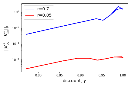
One may hypothesize that this is due to the fact that discount annealing directly operates on the true nonlinear dynamics whereas the other baselines (LQR and control), find the optimal controller for an idealized linearization of the dynamics. Indeed, there is evidence to support this hypothesis. In Figure 3 presented in Appendix D, we plot the error between the policy returned by policy gradients, and the optimal LQR policy for the (damped) linearized system, as a function of the discount factor used in each iteration of the discount annealing algorithm. For small training radius, such as , for all . However, for larger radii (i.e ), we see that steadily increases as increases.
That is, as discount annealing increases the discount factor and the closed-loop trajectories explore regions of the state space where the dynamics are increasingly nonlinear, begins to diverge from . Moreover, at the conclusion of discount annealing achieves a lower cost, namely [15.2, 15.4] vs [16.5, 16.8] (here denotes [, ] over 5 trials) and larger , namely [0.769, 0.777] vs [0.702, 0.703], than , suggesting that the method has indeed adapted to the nonlinearity of the system. Similar observations as to the behavior of controllers fine tuned via policy gradient methods are predicted by the theoretical results from Qu et al. (2020).
5 Discussion
This works illustrates how one can provably stabilize a broad class of dynamical systems via a simple model-free procedure based off policy gradients. In line with the simplicity and flexibility that have made model-free methods so popular in practice, our algorithm works under relatively weak assumptions and with little knowledge of the underlying dynamics. Furthermore, we solve an open problem from previous work (Fazel et al., 2018) and take a step towards placing model-free methods on more solid theoretical footing. We believe that our results raise a number of interesting questions and directions for future work.
In particular, our theoretical analysis states that discount annealing returns a controller whose stability properties are similar to those of the optimal LQR controller for the system’s Jacobian linearization. We were therefore quite surprised when in experiments, the resulting controller had a significantly better radius of attraction than the exact optimal LQR and controllers for the linearization of the dynamics. It is an interesting and important direction for future work to gain a better understanding of exactly when and how model-free procedures are adaptive to the nonlinearities of the system and improve upon these model-based baselines. Furthermore, for our analysis of nonlinear systems, we require access to damped system trajectories. It would be valuable to understand whether this is indeed necessary or whether our analysis could be extended to work without access to damped trajectories.
As a final note, in this work we reduce the problem of stabilizing dynamical systems to running policy gradients on a discounted LQR objective. This choice of reducing to LQR was in part made for simplicity to leverage previous analyses. However, it is possible that overall performance could be improved if rather than reducing to LQR, we instead attempted to run a model-free method that directly tries to optimize a robust control objective (which explicitly deals with uncertainty in the system dynamics). We believe that understanding these tradeoffs in objectives and their relevant sample complexities is an interesting avenue for future inquiry.
Acknowledgments
We would like to thank Peter Bartlett for many helpful conversations and comments throughout the course of this project, and Russ Tedrake for support with the numerical experiments. JCP is supported by an NSF Graduate Research Fellowship. MS is supported by an Open Philanthropy Fellowship grant. JU is supported by the National Science Foundation, Award No. EFMA-1830901, and the Department of the Navy, Office of Naval Research, Award No. N00014-18-1-2210.
References
- Abbasi-Yadkori and Szepesvári [2011] Yasin Abbasi-Yadkori and Csaba Szepesvári. Regret bounds for the adaptive control of linear quadratic systems. In Proceedings of the 24th Annual Conference on Learning Theory, pages 1–26, 2011.
- Andrychowicz et al. [2020] OpenAI: Marcin Andrychowicz, Bowen Baker, Maciek Chociej, Rafal Jozefowicz, Bob McGrew, Jakub Pachocki, Arthur Petron, Matthias Plappert, Glenn Powell, Alex Ray, et al. Learning dexterous in-hand manipulation. The International Journal of Robotics Research, 39(1):3–20, 2020.
- Callier and Desoer [2012] Frank M Callier and Charles A Desoer. Linear system theory. Springer Science & Business Media, 2012.
- Chen and Hazan [2021] Xinyi Chen and Elad Hazan. Black-box control for linear dynamical systems. In Conference on Learning Theory, pages 1114–1143. PMLR, 2021.
- Cohen et al. [2019] Alon Cohen, Tomer Koren, and Yishay Mansour. Learning linear-quadratic regulators efficiently with only sqrt(t) regret. In International Conference on Machine Learning, pages 1300–1309. PMLR, 2019.
- Dean et al. [2018] Sarah Dean, Horia Mania, Nikolai Matni, Benjamin Recht, and Stephen Tu. Regret bounds for robust adaptive control of the linear quadratic regulator. In Advances in Neural Information Processing Systems, pages 4188–4197, 2018.
- Dean et al. [2019] Sarah Dean, Horia Mania, Nikolai Matni, Benjamin Recht, and Stephen Tu. On the sample complexity of the linear quadratic regulator. Foundations of Computational Mathematics, pages 1–47, 2019.
- Faradonbeh et al. [2018a] Mohamad Kazem Shirani Faradonbeh, Ambuj Tewari, and George Michailidis. Finite-time adaptive stabilization of linear systems. IEEE Transactions on Automatic Control, 64(8):3498–3505, 2018a.
- Faradonbeh et al. [2018b] Mohamad Kazem Shirani Faradonbeh, Ambuj Tewari, and George Michailidis. On optimality of adaptive linear-quadratic regulators. arXiv preprint arXiv:1806.10749, 2018b.
- Faradonbeh et al. [2019] Mohamad Kazem Shirani Faradonbeh, Ambuj Tewari, and George Michailidis. Randomized algorithms for data-driven stabilization of stochastic linear systems. In 2019 IEEE Data Science Workshop (DSW), pages 170–174. IEEE, 2019.
- Fazel et al. [2018] Maryam Fazel, Rong Ge, Sham Kakade, and Mehran Mesbahi. Global convergence of policy gradient methods for the linear quadratic regulator. In International Conference on Machine Learning, pages 1467–1476. PMLR, 2018.
- Feng and Lavaei [2020] Han Feng and Javad Lavaei. Escaping locally optimal decentralized control polices via damping. In 2020 American Control Conference (ACC), pages 50–57. IEEE, 2020.
- Fiechter [1997] Claude-Nicolas Fiechter. Pac adaptive control of linear systems. In Proceedings of the tenth annual conference on Computational learning theory, pages 72–80, 1997.
- Flaxman et al. [2005] Abraham D. Flaxman, Adam Tauman Kalai, and H. Brendan McMahan. Online convex optimization in the bandit setting: gradient descent without a gradient. In Proceedings of the Sixteenth Annual ACM-SIAM Symposium on Discrete Algorithms, SODA ’05, page 385–394, USA, 2005. Society for Industrial and Applied Mathematics.
- Hazan et al. [2020] Elad Hazan, Sham Kakade, and Karan Singh. The nonstochastic control problem. In Algorithmic Learning Theory, pages 408–421. PMLR, 2020.
- Kakade et al. [2020] Sham Kakade, Akshay Krishnamurthy, Kendall Lowrey, Motoya Ohnishi, and Wen Sun. Information theoretic regret bounds for online nonlinear control. In Advances in Neural Information Processing Systems, volume 33, pages 15312–15325, 2020.
- Kingma and Ba [2014] Diederik P Kingma and Jimmy Ba. Adam: A method for stochastic optimization. arXiv preprint arXiv:1412.6980, 2014.
- Lamperski [2020] Andrew Lamperski. Computing stabilizing linear controllers via policy iteration. In 2020 59th IEEE Conference on Decision and Control (CDC), pages 1902–1907. IEEE, 2020.
- Laurent and Massart [2000] Beatrice Laurent and Pascal Massart. Adaptive estimation of a quadratic functional by model selection. Annals of Statistics, pages 1302–1338, 2000.
- Lewis et al. [2003] Frank L Lewis, Darren M Dawson, and Chaouki T Abdallah. Robot manipulator control: theory and practice. CRC Press, 2003.
- Malik et al. [2019] Dhruv Malik, Ashwin Pananjady, Kush Bhatia, Koulik Khamaru, Peter Bartlett, and Martin Wainwright. Derivative-free methods for policy optimization: Guarantees for linear quadratic systems. In The 22nd International Conference on Artificial Intelligence and Statistics, pages 2916–2925. PMLR, 2019.
- Mania et al. [2019] Horia Mania, Stephen Tu, and Benjamin Recht. Certainty equivalence is efficient for linear quadratic control. In Advances in Neural Information Processing Systems, pages 10154–10164, 2019.
- Mnih et al. [2015] Volodymyr Mnih, Koray Kavukcuoglu, David Silver, Andrei A Rusu, Joel Veness, Marc G Bellemare, Alex Graves, Martin Riedmiller, Andreas K Fidjeland, Georg Ostrovski, et al. Human-level control through deep reinforcement learning. Nature, 518(7540):529–533, 2015.
- Mohammadi et al. [2020] Hesameddin Mohammadi, Mahdi Soltanolkotabi, and Mihailo R Jovanović. On the linear convergence of random search for discrete-time lqr. IEEE Control Systems Letters, 5(3):989–994, 2020.
- Mohammadi et al. [2021] Hesameddin Mohammadi, Armin Zare, Mahdi Soltanolkotabi, and Mihailo R Jovanovic. Convergence and sample complexity of gradient methods for the model-free linear quadratic regulator problem. IEEE Transactions on Automatic Control, 2021.
- Parrilo [2003] Pablo A Parrilo. Semidefinite programming relaxations for semialgebraic problems. Mathematical programming, 96(2):293–320, 2003.
- Paszke et al. [2019] Adam Paszke, Sam Gross, Francisco Massa, Adam Lerer, James Bradbury, Gregory Chanan, Trevor Killeen, Zeming Lin, Natalia Gimelshein, Luca Antiga, et al. Pytorch: An imperative style, high-performance deep learning library. arXiv preprint arXiv:1912.01703, 2019.
- Peng et al. [2018] Xue Bin Peng, Marcin Andrychowicz, Wojciech Zaremba, and Pieter Abbeel. Sim-to-real transfer of robotic control with dynamics randomization. In 2018 IEEE International Conference on Robotics and Automation (ICRA), pages 3803–3810, 2018. doi: 10.1109/ICRA.2018.8460528.
- Perdomo et al. [2021] Juan C. Perdomo, Max Simchowitz, Alekh Agarwal, and Peter L. Bartlett. Towards a dimension-free understanding of adaptive linear control. In Conference on Learning Theory, volume 134 of Proceedings of Machine Learning Research, pages 3681–3770. PMLR, 2021.
- Prajna et al. [2004] Stephen Prajna, Pablo A Parrilo, and Anders Rantzer. Nonlinear control synthesis by convex optimization. IEEE Transactions on Automatic Control, 49(2):310–314, 2004.
- Qu et al. [2020] Guannan Qu, Chenkai Yu, Steven Low, and Adam Wierman. Combining model-based and model-free methods for nonlinear control: A provably convergent policy gradient approach. arXiv preprint arXiv:2006.07476, 2020.
- Rantzer [2001] Anders Rantzer. A dual to lyapunov’s stability theorem. Systems & Control Letters, 42(3):161–168, 2001.
- Sastry [2013] Shankar Sastry. Nonlinear systems: analysis, stability, and control, volume 10. Springer Science & Business Media, 2013.
- Sastry and Bodson [2011] Shankar Sastry and Marc Bodson. Adaptive control: stability, convergence and robustness. Courier Corporation, 2011.
- Silver et al. [2016] David Silver, Aja Huang, Chris J Maddison, Arthur Guez, Laurent Sifre, George Van Den Driessche, Julian Schrittwieser, Ioannis Antonoglou, Veda Panneershelvam, Marc Lanctot, et al. Mastering the game of go with deep neural networks and tree search. Nature, 529(7587):484–489, 2016.
- Simchowitz and Foster [2020] Max Simchowitz and Dylan Foster. Naive exploration is optimal for online lqr. In International Conference on Machine Learning, pages 8937–8948. PMLR, 2020.
- Simchowitz et al. [2020] Max Simchowitz, Karan Singh, and Elad Hazan. Improper learning for non-stochastic control. In Conference on Learning Theory, pages 3320–3436. PMLR, 2020.
- Sontag [1999] Eduardo D Sontag. Nonlinear feedback stabilization revisited. In Dynamical Systems, Control, Coding, Computer Vision, pages 223–262. Springer, 1999.
- Sontag [2009] Eduardo D. Sontag. Stability and feedback stabilization. Springer New York, New York, NY, 2009. ISBN 978-0-387-30440-3. doi: 10.1007/978-0-387-30440-3_515.
- Tu and Recht [2019] Stephen Tu and Benjamin Recht. The gap between model-based and model-free methods on the linear quadratic regulator: An asymptotic viewpoint. In Conference on Learning Theory, pages 3036–3083. PMLR, 2019.
- Zhang et al. [2021] Kaiqing Zhang, Xiangyuan Zhang, Bin Hu, and Tamer Başar. Derivative-free policy optimization for risk-sensitive and robust control design: implicit regularization and sample complexity. arXiv preprint arXiv:2101.01041, 2021.
- Zhou and Doyle [1998] Kemin Zhou and John Comstock Doyle. Essentials of robust control, volume 104. Prentice Hall, 1998.
- Zhou et al. [1996] Kemin Zhou, John Comstock Doyle, Keith Glover, et al. Robust and optimal control, volume 40. Prentice hall New Jersey, 1996.
Appendix A Deferred Proofs and Analysis for the Linear Setting
Preliminaries on Linear Quadratic Control.
The cost a state-feedback controller is intimately related to the solution of the discrete-time Lyapunov equation. Given a stable matrix and a symmetric positive definite matrix , we define to be the unique solution (over ) to the matrix equation,
A classical result in Lyapunov theory states that . Recalling our earlier definition, for a controller such that is stable, we let , where are the cost matrices for the LQR problem defined in Definition 2.1. As a special case, we let where is the optimal controller for the undiscounted LQR problem. Using these definitions, we have the following facts:
Fact A.1.
if and only if is a stable matrix.
Fact A.2.
If then for all , . Furthermore,
Employing these identities, we can now restate and prove Lemma 2.1:
Lemma 2.1.
For all such that , .
Proof.
Therefore, since LQR with a discount factor is equivalent to LQR with damped dynamics, it follows that for , (noisy) policy gradients initialized at the zero controller converges to the global optimum of the discounted LQR problem. The following lemma is essentially a restatement of the finite sample convergence result for gradient descent on LQR (Theorem 31) from Fazel et al. [2018], where we have set and as in the discount annealing algorithm. We include the proof of this result in Section A.2 for the sake of completeness.
Lemma A.3 (Fazel et al. [2018]).
For such that , define (noisy) policy gradients as the procedure which computes updates according to,
for some matrix . There exists a choice of a constant step size and a fixed polynomial,
such that if the following inequality holds for all ,
| (A.1) |
then whenever
With this lemma, we can now present the proof of Theorem 1.
A.1 Discount annealing on linear systems: Proof of Theorem 1
We organize the proof into two main parts. First, we prove statements and by an inductive argument. Then, having already proved part in the main body of the paper, we finish the proof by establishing the stability guarantees of the resulting controller outlined in part .
A.1.1 Proof of and
Base case.
Recall that at iteration of discount annealing, policy gradients is initialized at and (in the case of linear systems) computes updates according to:
From Lemma A.3, if and
| (A.2) |
where then policy gradients will converge to a such that after many iterations.
By our choice of discount factor, we have that . Furthermore, since , then the condition outlined in Eq. A.2 holds and policy gradients achieves the desired guarantee when .
The correctness of binary search at iteration follows from Lemma C.6. In particular, we instantiate the lemma with of the LQR objective, which is nondecreasing in by definition, and . The algorithm requires auxiliary values and which we can always compute by using to estimate the cost to precision (recall that for any and ). The last step needed to apply the lemma is to lower bound the width of the feasible region of ’s which satisfy the desired criterion that .
Let be such that . Such a is guaranteed to exist since is nondecreasing in and it is a continuous function for all . By the calculation from the proof of part presented in the main body of the paper, for
we have that . By monotonicity and continuity of , when restricted to , all satisfy . Moreover,
where the last line follows from the fact that and that the trace of a PSD matrix is always at least as large as the operator norm. Lastly, since , by the guarantee of policy gradients, we have that for , . Therefore, for :
Hence the width of the feasible region is at least .
Inductive step.
To show that policy gradients achieves the desired guarantee at iteration , we can repeat the exact same argument as in the base case. The only difference is that the need to argue that the cost of the initial controller is uniformly bounded across iterations. By the inductive hypothesis on the success of the binary search algorithm at iteration , we have that,
Hence, by Lemma A.3, policy gradients achieves the desired guarantee using many queries to as long as is less than .
Likewise, the argument for the correctness of the binary search procedure is identical to that of the base case. Because of the success of policy gradients and binary search at the previous iteration, we can upper bound, by and get a uniform lower bound on the width of the feasible region.
A.1.2 Proof of
After halting, we see that discount annealing returns a controller satisfying the stated condition from Step 2 requiring that,
Here, we have used A.2 to rewrite as for (and likewise for ). Since , we conclude that . Now, by properties of the Lyapunov equation (see Lemma A.5) the following holds for :
Hence, we conclude that,
A.2 Convergence of policy gradients for LQR: Proof of Lemma A.3
Proof.
Note that, by Lemma 2.1, proving the above result for is the same as proving it for . We start by defining the following idealized updates,
From Lemmas 13, 24, and 25 from Fazel et al. [2018], there exists a fixed polynomial,
Such that, for , the following inequality holds,
where and is the sequence of states generated by the controller . Therefore, if and satisfy,
| (A.3) |
then, as long as , this following inequality also holds:
The proof then follows by unrolling the recursion and simplifying. We now focus on establishing Eq. A.3. By Lemma 27 in Fazel et al. [2018], if
where is a fixed polynomial , then
where . Therefore, Eq. A.3 holds if
The exact statement follows from using and by Lemma 13 in [Fazel et al., 2018] and taking the polynomial in the proposition statement to be the minimum of and . ∎
A.3 Impossibility of reward shaping: Proof of Proposition 2.2
Proof.
Consider the linear dynamical system with dynamics matrices,
where is a parameter to be chosen later. Note that a linear dynamical system of these dimensions is controllable (and hence stabilizable) [Callier and Desoer, 2012], since the matrix
is full rank. For any controller , the closed loop system has the form,
By Gershgorin’s circle theorem, has an eigenvalue which satisfies,
Therefore, any controller for which the closed-loop system is stable must have the property that,
Using this observation and A.2, for any discount factor , a stabilizing controller must satisfy,
In the above calculation, we have used the identity as well as the assumption that is positive definite. Next, we observe that for a discount factor , where as chosen in the initial iteration of our algorithm, the cost of the 0 controller has the following upper bound:
Using standard Lyapunov arguments (see for example Section D.2 in Perdomo et al. [2021]) the sum in the last line is a geometric series and is equal to some function , which depends only on and , for all . Using this calculation, it follows that
Hence, for any , and discount factor , we can choose small enough such that,
implying that the optimal controller for the discounted problem cannot be stabilizing for . ∎
A.4 Auxiliary results for linear systems
Proposition A.4.
Let be a stable matrix and define , then for defined as
the following holds for and :
Proof.
The proof is a direct consequence of Proposition C.7 in Perdomo et al. [2021]. In particular, we use their results for the trace norm and use the following substitutions,
where and are defined as in Perdomo et al. [2021]. Note that for satisfying,
we get that,
Therefore, Proposition C.7 states that, for ,
Lastly, noting that,
we have that and . Therefore, since , in order to apply Proposition C.7 from Perdomo et al. [2021] it suffices for to satisfy,
∎
Lemma A.5 (Lemma D.9 in Perdomo et al. [2021]).
Let be a stable matrix, , and define . Then, for all ,
Lemma A.6.
Let be a stable matrix and define where . Then, for any matrix such that it holds that for all
Proof.
Expanding out, we have that
where in the second line we have used properties of the Lyapunov function, Lemma A.5. Next, we observe that
where we have again used Lemma A.5 to conclude that . Note that the exact same calculation holds for . Hence, we can conclude that for such that ,
Using the fact that, and that , we get that,
which finishes the proof. ∎
Appendix B Deferred Proofs and Analysis for the Nonlinear Setting
Establishing Lyapunov functions. Our analysis for nonlinear systems begins with the observation that any state-feedback controller which achieves finite cost on the -discounted LQR problem has an associated value function which can be used as a Lyapunov function for the -damped nonlinear dynamics, for small enough initial states. We present the proof of this result in Section B.3.
Lemma B.1.
Let . Then, for all such that,
the following inequality holds:
Using this observation, we can then show that any controller which has finite discounted LQR cost is exponentially stabilizing over states in a sufficiently small region of attraction.
Lemma B.2.
Assume and define be the sequence of states generated according to where . If is such that,
then for all and for defined as above,
-
a)
The norm of the state is bounded by
(B.1) -
b)
The norms of and are bounded by
(B.2) (B.3)
Proof.
Relating to its Jacobian Linearization. Having established how any controller that achieves finite LQR cost is guaranteed to be stabilizing for the nonlinear system, we now go a step further and illustrate how this stability guarantee can be used to prove that the difference in costs and gradients between and its Jacobian linearization are guaranteed to be small.
Proposition 3.3 (restated).
Assume . Then,
-
a)
If , then
-
b)
If , then,
Proof.
Due to our assumption on , we have that,
Therefore, we can apply Lemma B.5 to conclude that,
Next, we multiply both sides by , take expectations, and apply Jensen’s inequality to get that,
Given our definitions of the linear objective in Definition 2.1, we have that,
for all . Therefore, we can rewrite the inequality above as,
The second part of the proposition uses the same argument as part a, but this time employing Lemma B.6 to bound the difference in gradients (pointwise). ∎
In short, this previous lemma states that if the cost on the linear system is bounded, then the costs and gradients between the nonlinear objective and its Jacobian linearization are close. We can also prove the analogous statement which establishes closeness while assuming that the cost on the nonlinear system is bounded.
Lemma B.3.
Let be such that .
-
1.
If , then .
-
2.
If , then
Proof.
The lemma is a consequence of combining Proposition 3.3 and Proposition C.5. In particular, from Proposition C.5 if , then
However, since , we conclude that . Having shown that the linear cost is bounded, we can now plug in Proposition 3.3. In particular, if
then, Proposition 3.3 states that
To prove the second part of the statement, we again use Proposition 3.3. In particular, since
we can hence conclude that
∎
B.1 Discount annealing on nonlinear systems: Proof of Theorem 2
As in Theorem 1, we first prove parts and by induction and then prove parts and separately.
B.1.1 Proof of and
Base case. As before, at each iteration of discount annealing, policy gradients is initialized at and computes updates according to,
To prove correctness, we show that the noisy gradients on the nonlinear system are close to the true gradients on the linear system. That is,
| (B.4) |
where is again a fixed polynomial from Lemma A.3.
Consider the first iteration of discount annealing, by choice of , we have that . Therefore, by Proposition 3.3 if
it must hold that . Likewise, if we choose the tolerance parameter in then we have that
By the triangle inequality, the inequality in Eq. B.4 holds for and . However, because Lemma A.3 shows that policy gradients is a descent method, that is for all , Eq. B.4 also holds for all for the same choice of and tolerance parameter for . By guarantee of Lemma A.3, for , policy gradients achieves the guarantee outlined in Step 2 using at most many queries.
To prove that random search achieves the guarantee outlines in Step 4 at iteration 0 of discount annealing, we appeal to Lemma C.7. In particular, we instantiate the lemma with , , . As before, the algorithm requires values and . These can be estimated via two calls to with tolerance parameter .
To show the lemma applies we only need to lower bound the width of feasible such that
| (B.5) |
From the guarantee from policy gradients, we know that . Furthermore, from the proof of Theorem 1, we know that there exists satisfying, , such that for all
| (B.6) |
To finish the proof of correctness, we show that any that satisfies Eq. B.6 must also satisfy Eq. B.5. In particular, since and for
it holds that and . Using these two inequalities along with Eq. B.6 implies that Eq. B.5 must also hold. Therefore, the width of the feasible region is at least and random search must return a discount factor using at most 1 over this many iterations by Lemma C.7.
Inductive step.
To show that policy gradients converges, we can use the exact same argument as when arguing the base case where instead of referring to and we use and . In particular, we can reuse the same argument as in the base case, but need to ensure that is that is uniformly bounded.
To prove this, from the inductive hypothesis on the correctness of binary search at previous iterations, we know that . Again by the inductive hypothesis, at time step policy gradients achieves the desired guarantee from Step 2, implying that . By choice of this implies that
and hence . Now, we can apply Lemma B.3 to conclude that for and
it holds that and hence . Therefore, .
Similarly, the inductive step for the random search procedure follows from noting that the exact same argument can be repeated by replacing with and with since (by the inductive hypothesis) .
B.1.2 Proof of
By the guarantee from Step 2, the algorithm returns a which satisfies the following guarantee on the linear system:
Therefore, . Now by, Lemma B.2, the following holds,
for and all such that
B.1.3 Proof of
The bound for the number of subproblems solved by the discount annealing algorithms is similar to that of the linear case. The crux of the argument for part is to show that any such that
the following inequality must also hold: . Once we’ve lower bounded the cost on the linear system, we can repeat the same argument as in Theorem 1. Since the cost on the linear system in nondecreasing in , it must be the case that satisfies
Here, we have again we have used the calculation that,
which follows from the guarantee that (for our choice of ) policy gradients on the nonlinear system converges to a near optimal controller for the system’s Jacobian linearization. Hence, as in the linear setting, we conclude that and discount annealing achieves the same rate as for linear systems.
We now focus on establishing that . By guarantee from policy gradients, we have that . Therefore, by Proposition 3.3 since
it holds that .
Next, we show that is also small. In particular, the previous statement, together with the guarantee from Step 4, implies that
Therefore, for , Lemma B.3 implies that if,
it holds that . Hence, if we get that . Using again the fact that for all we hence conclude that
which finished the proof of the fact that .
B.2 Relating costs and gradients to the linear system: Proof of Proposition 3.3
In order to relate the properties of the nonlinear system to its Jacobian linearization, we employ the following version of the performance difference lemma.
Lemma B.4 (Performance Difference).
Assume and define be the sequence of states generated according to where . Then,
Proof.
From the definition of the relevant objectives, and A.2, we get that,
| (B.7) |
where in the last line we have used the fact that . The proof then follows from the following two observations. First, by definition of state sequence, ,
Second, since is the solution to a Lyapunov equation,
Plugging these last two lines into Eq. B.7, we get that is equal to,
∎
B.2.1 Establishing similarity of costs
The following lemma follows by bounding the terms appearing in the performance difference lemma.
Lemma B.5 (Similarity of Costs).
Assume and define be the sequence of states generated according to where . For such that,
then,
Proof.
We begin with the following observation. Due to our assumption on , we can use Lemma B.2 to conclude that for all , the following relationship holds for ,
| (B.8) |
Now, from the performance difference lemma (Lemma B.4), we get that is equal to:
Therefore, the difference can be bounded by,
| (B.9) |
Now, we analyze each of and separately. For , by Lemma 3.1, and the fact that ,
where in the last line, we have used our assumption on the initial state and Lemma B.2. Moving onto , we use the triangle inequality to get that
For the second term above, by Lemma A.5 and Lemma B.2, we have that
Lastly, we bound the first term by again using Lemma B.2,
Therefore, is bounded by . Going back to Eq. B.9, we can combine our bounds on and to conclude that,
Using the fact that and , we get that
∎
B.2.2 Establishing similarity of gradients
Much like the previous lemma which bounds the costs between the linear and nonlinear system via the performance difference lemma, this next lemma differentiates the performance difference lemma to bound the difference between gradients.
Lemma B.6.
Assume . If is such that
then,
Proof.
Using the variational definition of the Frobenius norm,
where is the directional derivative operator in the direction . The argument follows by bounding the directional derivative appearing above. From the performance difference lemma, Lemma B.4, we have that
Each term appearing in the sum above can be decomposed into the following three terms,
In order to bound each of these three terms, we start by bounding the directional derivatives appearing above. Throughout the remainder of the proof, we will make repeated use of the following inequalities which follow from Lemma 3.1, Lemma B.2, and our assumption on . For all ,
| (B.10) | ||||
| (B.11) |
Lemma B.7 (Bounding .).
Let be the sequence of states generated according to . Under the same assumptions as in Lemma B.6, for all
Proof.
Taking derivatives, we get that
Since, , we can rewrite the expression above as,
| (B.12) | ||||
Next, we compute ,
Plugging in our earlier calculation for , we get that the following recursion holds for ,
| (B.13) | ||||
| (B.14) |
Using the shorthand introduced above, we can re-express the recursion as,
Unrolling this recursion, with the base case that , we get that
Therefore,
| (B.15) |
Next, we prove that each matrix is stable so that the product of the is small. By Lemma 3.1 and our earlier inequalities,Eq. B.10 & Eq. B.11, we have that,
| (B.16) |
where we have used our initial condition on . Therefore, where for all . By definition of the operator norm, Lemma A.6, and the fact that :
Then, using our bound on from Eq. B.16, and Lemma B.2, we bound (defined in Eq. B.13) as,
Returning to our earlier bound on in Eq. B.15, we conclude that,
concluding the proof. ∎
Using this, we can now return to bounding .
Lemma B.8 (Bounding ).
For all , the following bound holds:
Proof.
From Eq. B.12, is less than,
Again using the assumption on the nonlinear dynamics, we can bound the gradient terms as in Eq. B.16 and get that is no larger than,
Seeing as how our upper bound on in Lemma B.7 is always larger than the bound for in Eq. B.10, we can bound by the former. Consequently,
∎
Finally, we bound .
Lemma B.9 (Bounding ).
The following bound holds:
Proof.
By definition of the discrete time Lyapunov equation,
Therefore, the directional derivative satisfies another Lyapunov equation,
implying that . By properties of the Lyapunov equation,
Therefore, to bound it suffices to bound, . Using the fact that and that , a short calculation reveals that,
which together with our previous bound on implies that,
∎
With Lemmas B.7, B.8 and B.9 in place, we now return to bounding terms .
Bounding
Bounding
Bounding .
Wrapping up
Therefore,
And hence,
∎
B.3 Establishing Lyapunov functions: Proof of Lemma B.1
Proof.
To be concise, we use the shorthand, . We start by expanding out,
By the AM-GM inequality for vectors, the following holds for any ,
Combining these two relationships, we get that,
| (B.18) |
Next, by properties of the Lyapunov function Lemma A.5, we have that
Letting, , we can plug in the previous expression into Eq. B.18 and optimize over to get that,
where we have dropped a factor of from the last two terms since . Next, the proof follows by noting that this following inequality is satisfied,
| (B.19) |
whenever,
| (B.20) |
Therefore, assuming the inequality above Eq. B.20, we get our desired result showing that
We conclude the proof by showing that Eq. B.20 is satisfied for all small enough. In particular, using our bounds on from Lemma 3.1, if ,
Since , in order for Eq. B.20 to hold, it suffices for to satisfy
Using the fact that , we can simplify upper bound on to be,
Note that this condition is always implied by the condition on in the statement of the proposition. ∎
B.4 Bounding the nonlinearity: Proof of Lemma 3.1
Since the origin is an equilibrium point, , we can rewrite as,
for some function . Taking gradients,
Hence, for all such that the smoothness assumption holds, we get that
Next, by Taylor’s theorem,
and since , we can bound,
Appendix C Implementing , , and Search Algorithms
We conclude by discussing the implementations and relevant sample complexities of the noisy gradient and function evaluation methods, and . We then use these to establish the runtime and correctness of the noisy binary and random search algorithms.
We remark that throughout our analysis, we have assumed that and succeed with probability 1. This is purely for the sake of simplifying our presentation. As established in Fazel et al. [2018], the relevant estimators in this section all return approximate solutions with probability , where factors into the sample complexity polynomially. Therefore, it is easy to union bound and get a high probability guarantee. We omit these union bounds for the sake of simplifying the presentation.
C.1 Implementing
Linear setting.
From the analysis in Fazel et al. [2018], we know that if , then
| (C.1) |
where is the length , finite horizon cost of :
More formally, if is smaller than a constant , Lemma 26 from Fazel et al. [2018] states that it suffices to set and to be polynomials in and in order to have an -approximate estimate of with high probability.
On the other hand, if is larger than (recall that the costs should never be larger than some universal constant times during discount annealing), the following lemma proves we can detect that this is the case by setting and to be polynomials in and . This argument follows from the following two lemmas:
Lemma C.1.
Fix a constant , and take . Then for any (possibly even with ),
Setting for some universal constant , we get that all calls to the oracle during discount annealing can be implemented with polynomially many samples. Using standard arguments, we can boost this result to hold with high probability by running independent trials, where is again a polynomial in the relevant problem parameters.
Nonlinear setting.
Next, we sketch why the same estimator described in Eq. C.1 also works in the nonlinear case if we replace with the analogous finite horizon cost, , for the nonlinear objective. By Lemma B.3 and Proposition 3.3 if the nonlinear cost is small, then costs on the nonlinear system and the linear system are pointwise close. Therefore, previous concentration analysis for the linear setting from Fazel et al. [2018] can be easily carried over in order to implement where and are depend polynomially on the relevant problem parameters.
On the other hand if the nonlinear cost is large, then the cost on the linear system must also be large. Recall that if the linear cost was bounded by a constant, then the costs of both systems would be pointwise close by Proposition 3.3. By Proposition C.5, we know that the -step nonlinear cost is lower bounded by the cost on the linear system. Since we can always detect that the cost on the linear system is larger than a constant using polynomially many samples as per Lemma C.1, with high probability we can also detect if the cost on the nonlinear system is large using again only polynomially many samples.
C.2 Implementing
Linear setting.
Just like in the case of , Fazel et al. [2018] (Lemma 30) prove that
| (C.2) |
where and only need to be made polynomial large in the relevant problem parameter and in order to get an accurate approximation of the gradient. Note that we can safely assume that is finite (and hence the gradient is well defined) since we can always run the test outlined in Lemma C.1 to get a high probability guarantee of this fact. In order to approximate the gradients , one can employ standard techniques from Flaxman et al. [2005]. We refer the interested reader to Appendix D in Fazel et al. [2018] for further details.
Nonlinear setting.
Lastly, we remark that, as in the case of , Lemma B.6 establishes that the gradients between the linear and nonlinear system are again pointwise close if the cost on the linear system is bounded. In the proof of Theorem 2, we established that during all iterations of discount annealing, the cost on the linear system during executions of policy gradients is bounded by . Therefore, the analysis from Fazel et al. [2018] can be ported over to show that -approximate gradients of the nonlinear system can be computed using only polynomially many samples in the relevant problem parameters.
C.3 Auxiliary results
Lemma C.2.
Fix any constant . Then, for
the following relationship holds
where may be infinite.
Proof.
We have two cases. In the first case has an eigenvalue . Letting denote such a corresponding eigenvector of unit norm, one can verify that , which is at least by assumption.
In the second case, is stable, so exists and its trace is (see A.2). Then, for ,
we show that if , then .
To show this, observe that if , then . Therefore, by the pidgeonhole principle (and the fact that ), there exists some such that . Since , this means that as well. Therefore, letting denote the -step value function from Eq. C.3, the identity means that
where in the last line we used . This completes the proof. ∎
Lemma C.3.
Let then, .
Proof.
The statement is clearly true for , therefore we focus on the case where . Without loss of generality, we can take to be the first basis vector and let where . From these simplifications, we observe that is equal in distribution to the following random variable,
where each is a chi-squared random variable. Using this equivalency, we have that for arbitrary ,
Setting , we get that,
From a direct computation,
To bound the last term, if is a chi-squared random variable with degrees of freedom, by Lemma 1 in Laurent and Massart [2000],
Setting we get that . Substituting in , we conclude that,
which is greater than .99 for . ∎
Lemma C.1 (restated).
Fix a constant , and take . Then for any (possibly even with ),
Proof.
Observe that for the finite horizon value matrix , we have . We now observe that, since , it has a (possibly non-unique) top eigenvector for which
Since , Lemma C.3 ensures that . Hence,
The bound now follows from invoking Lemma C.2 to lower bound provided .
∎
In the following lemmas, we define to be the following matrix where is any state-feedback controller.
| (C.3) |
Similarly, we let be the horizon cost of the nonlinear dynamical system:
| (C.4) | |||
| (C.5) |
And again overloading notation like before, we let .
Lemma C.4.
Fix a horizon , constant , , and suppose that
Furthermore, define . Then, if , it holds that
Proof.
Fix a constant to be selected. Throughout, we use the shorthand We consider two cases.
Case 1:
The initial point is such that it is always the case that for all and . Observe that we can write the nonlinear dynamics as
where . We now write:
Then, setting ,
where (a) the last inequality uses the elementary inequality for any pair of vectors and , and (b) the last inequality recognizes how
for defined above in Eq. C.3. Moreover, for any ,
Now, because , Lemma 3.1 lets use bound , where we adopt the previously defined shorthand . Therefore,
Next, if ,
In particular, selecting (which ensures by the conditions of the lemma), it holds that,
Case 2:
The initial point is such that it is always the case that either for all or . Therefore, in either case, . For our choice of , this gives
Combining the cases, we have
∎
Proposition C.5.
Let be a given (integer) tolerance and be defined as in Lemma C.4. Then, for , , and satisfying,
| (C.6) |
it holds that:
Moreover, for ,
C.4 Search analysis
Noisy Binary Search Require: and as defined in Lemma C.6. Initialize: , for , For 1. Query where 2. If , update and 3. Else if, , update and 4. Else, break and return Noisy Random Search Require: , as defined in Lemma C.7. Initialize: for , For 1. Sample uniformly at random from 2. Query 3. If , break and return ,
Lemma C.6.
Let be a nondecreasing function over the unit interval. Then, given such that and for which there exist such that for all , , binary search as defined in Figure 2 returns a value such that in at most many iterations where .
Lemma C.7.
Let be a function over the unit interval. Then, given given such that and for which there exist such that for all , , with probability , noisy random search as defined in Figure 2 returns a value such that in at most many iterations where .
The analysis of the correctness and runtime of this classical algorithms for search problems in 1 dimension are standard. We omit the proofs for the sake of concision.
Appendix D Additional Experiments
D.1 Cart-pole dynamics
The state of the cart-pole is given by , where and denote the horizontal position and velocity of the cart, and and denote the angular position and velocity of the pole, with corresponding to the upright equilibrium. The control input corresponds to the horizontal force applied to the cart. The continuous time dynamics are given by
where denotes the mass of the pole, the mass of the cart, the length of the pendulum, and acceleration due to gravity. For our experiments, we set all parameters to unity, i.e. .
D.2 synthesis
Consider the following linear system
| (D.1) |
where denotes an additive disturbance to the state transition, and denotes the so-called performance output. Notice that . The optimal controller minimizes the -norm of the closed-loop system from input to output , i.e. the smallest such that
holds for all , all , and . In essence, the optimal controller minimizes the effect of the worst-case disturbance on the cost. In this setting, additive disturbances serve as a crude (and unstructured) proxy for modeling error. We synthesize the optimal controller using Matlab’s hinfsyn function. For the system (D.1) with perfect state observation, we require only static state feedback to implement the controller.
D.3 Difference between LQR and discount annealing as a function of discount
In Figure 3 we plot the error between the policy returned by policy gradient and the optimal policy for the (damped) linearized system, as a function of the discount during the discount annealing process. Observe that for small radius of the ball of initial conditions (), the optimal controller from policy gradient remains very close to the exact optimal controller for the linearized system; however, for larger radius () the controller from policy gradient differs significantly.