This paper was converted on www.awesomepapers.org from LaTeX by an anonymous user.
Want to know more? Visit the Converter page.

Stabilizing Linear Systems under Partial Observability:
Sample Complexity and Fundamental Limits

Ziyi Zhang111Department of Electrical and Computer Engineering, Carnegie Mellon University. Email: ziyizhan@andrew.cmu.edu  Yorie Nakahira222Department of Electrical and Computer Engineering, Carnegie Mellon University. Email: ynakahir@andrew.cmu.edu   Guannan Qu333Department of Electrical and Computer Engineering, Carnegie Mellon University. Email: gqu@andrew.cmu.edu
Abstract

We study the problem of stabilizing an unknown partially observable linear time-invariant (LTI) system. For fully observable systems, leveraging an unstable/stable subspace decomposition approach, state-of-art sample complexity is independent from system dimension nn and only scales with respect to the dimension of the unstable subspace. However, it remains open whether such sample complexity can be achieved for partially observable systems because such systems do not admit a uniquely identifiable unstable subspace. In this paper, we propose LTS-P, a novel technique that leverages compressed singular value decomposition (SVD) on the “lifted” Hankel matrix to estimate the unstable subsystem up to an unknown transformation. Then, we design a stabilizing controller that integrates a robust stabilizing controller for the unstable mode and a small-gain-type assumption on the stable subspace. We show that LTS-P stabilizes unknown partially observable LTI systems with state-of-the-art sample complexity that is dimension-free and only scales with the number of unstable modes, which significantly reduces data requirements for high-dimensional systems with many stable modes.

1 Introduction

Learning-based control of unknown dynamical systems is of critical importance for many autonomous control systems [Beard et al., 1997; Li et al., 2022; Bradtke et al., 1994; Krauth et al., 2019; Dean S. Mania, 2020]. However, existing methods make strong assumptions such as open-loop stability, availability of initial stabilizing controller, and fully observable systems [Fattahi, 2021; Sarkar et al., 2019]. However, such assumptions may not hold in many autonomous control systems. Motivated by this gap, this paper focuses on the problem of stabilizing an unknown, partially-observable, unstable system without an initial stabilizing controller. Specifically, we consider the following linear-time-invariant (LTI) system:

xt+1=Axt+Butyt=Cxt+Dut+vt,\begin{split}x_{t+1}&=Ax_{t}+Bu_{t}\\ y_{t}&=Cx_{t}+Du_{t}+v_{t},\end{split} (1)

where xtnx_{t}\in\mathbb{R}^{n} and utdu,ytdyu_{t}\in\mathbb{R}^{d_{u}},y_{t}\in\mathbb{R}^{d_{y}} are the state, control input, and observed output at time step t{0,,T1}t\in\{0,\dots,T-1\}, respectively. The system also has additive observation noise vt𝒩(0,σv2I)v_{t}\sim\mathcal{N}(0,\sigma_{v}^{2}I).

While there are works studying system identification for partially observable LTI systems [Fattahi, 2021; Sun et al., 2020; Sarkar et al., 2019; Oymak and Ozay, 2018b; Zheng and Li, 2020], none of these works address the subsequent stabilization problem; in fact, many assume open-loop stability [Fattahi, 2021; Sarkar et al., 2019; Oymak and Ozay, 2018b]. Other adaptive control approaches can solve the learn-to-stabilize problem in (1) and achieve asymptotic stability guarantees [Pasik-Duncan, 1996; Petros A. Ioannou, 2001], but the results therein are asymptotic in nature and do not study the transient performance.

Recently, in the special case when C=IC=I, i.e. fully-ovservable LTI system, Chen and Hazan [2020] reveals that the transient performance during the learn-to-stabilize process suffers from exponential blow-up, i.e. the system state can blow up exponentially in the state dimension. This is mainly due to that in order to stabilize the system, system identification for the full system is needed, which takes at least nn samples on a single trajectory, during which the system could blow up exponentially for nn steps.

To relieve this problem, Hu et al. [2022] proposed a framework of separating the unstable component of the system and stabilizing the entire system by stabilizing the unstable subsystem. This reduces the sample complexity to only grow with the number of the unstable eigenvalues (as opposed to the full state dimension nn). This result was later extended to noisy setting in Zhang et al. [2024], and such a dependence on the number of unstable eigenvalues is the best sample complexity so far for the learn-to-stabilize problem in the fully observable case. Compared with this line of work, our work focuses on partially observable systems, which is fundamentally more difficult than the fully observable case. First, partially observable systems typically need a dynamic controller, which renders stable feedback controllers in the existing approach not applicable [Hu et al., 2022]. Second, the construction in “unstable subspace” in Hu et al. [2022] is not uniquely defined in the partially observable case. This is because the state and the A,B,CA,B,C matrices are not uniquely identifiable from the learner’s perspective, as any similarity transformation of the matrices can yield the same input-output behavior. Given the above discussions, we ask the following question:

Is it possible to stabilize a partially observable LTI system by only identifying an unstable component (to be properly defined) with a sample complexity independent of the overall state dimension?

Contribution. In this paper, we answer the above question in the affirmative. Firstly, we propose a novel definition of “unstable component” to be a low-rank version of the transfer function of the original system that only retains the unstable eigenvalues. Based on this unstable component, we propose LTS-P, which leverages compressed singular value decomposition (SVD) on a “lifted” Hankel matrix to estimate the unstable component. Then, we design a robust stabilizing controller for the unstable component, and show that it stabilizes the full system under a small-gain-type assumption on the HH_{\infty} norm of the stable component. Importantly, our theoretical analysis shows that the sample complexity of the proposed approach only scales with the dimension of unstable component, i.e. the number of unstable eigenvalues, as opposed to the dimension of the full state space. We also conduct simulations to validate the effectiveness of LTS-P, showcasing its ability to efficiently stabilize partially observable LTI systems.

Moreover, the novel technical ideas behind our approach are also of independent interest. We show that by using compressed singular value decomposition (SVD) on a properly defined lifted Hankel matrix, we can estimate the unstable component of the system. This is related to the classical model reduction [Dullerud and Paganini, 2000, Chapter 4.6], but our dynamics contain unstable modes with a blowing up Hankel matrix as opposed to the stable Hankel matrix in Dullerud and Paganini [2000] and the system identification results in Fattahi [2021]; Sarkar et al. [2019]; Oymak and Ozay [2018b]. Interestingly, the HH_{\infty} norm condition on the stable component, derived from the small gain theorem, is a necessary and sufficient condition for stabilization, revealing the required subspace to be estimated in order to stabilize the unknown systems. Such a result not only suggests the optimality of LTS-P but also informs the fundamental limit on stabilizability.

Related Work. Our work is mostly related to adaptive control, learn-to-control with known stabilizing controllers, learn-to-stabilize on multiple trajectories, and learn-to-stabilize on a single trajectory. In addition, we will also briefly cover system identification.

Adaptive control. Adaptive control enjoys a long history of study [Pasik-Duncan, 1996; Petros A. Ioannou, 2001; Chen and Astolfi, 2021]. Most classical adaptive control methods focus on asymptotic stability and do not provide finite sample analysis. The more recent work has started to study non-asymptotic sample complexity of adaptive control when a stabilizing controller is unknown [Chen and Hazan, 2020; Faradonbeh, 2017; Lee et al., 2023; Tsiamis and Pappas, 2021; Tu and Recht, 2018]. Specifically, the most typical strategy to stabilize an unknown dynamic system is to use past trajectory to estimate the system dynamics and then design the controller [Berberich et al., 2020; De Persis and Tesi, 2020; Liu et al., 2023]. Compared with those works, we can stabilize the system with fewer samples by identifying and stabilizing only the unstable component.

Learn to control with known stabilizing controller. Extensive research has been conducted on stabilizing LTI under stochastic noise [Bouazza et al., 2021; Jiang and Wang, 2002; Kusii, 2018; Li et al., 2022]. One branch of research uses the model-free approach to learn the optimal controller [Fazel et al., 2019; Jansch-Porto et al., 2020; Li et al., 2022; Wang et al., 2022; Zhang et al., 2020]. Those algorithms typically require a known stabilization controller as an initialization policy for the learning process. Another line of research utilizes the model-based approach, which requires an initial stabilizing controller to learn the system dynamics for controller design [Cohen et al., 2019; Mania et al., 2019; Plevrakis and Hazan, 2020; Zheng et al., 2020]. On the other hand, we focus on learn-to-stabilize. Our method can be used as the initial policy in these methods to remove their requirement on initial stabilizing controllers.

Learn-to-stabilize on multiple trajectories. There are also works that do not assume open-loop stability and learn the full system dynamics before designing a stabilizing controller while requiring Θ~(poly(n))\widetilde{\Theta}(\text{poly}(n)) complexity [Dean S. Mania, 2020; Tu and Recht, 2018; Zheng and Li, 2020]. Recently, a model-free approach via the policy gradient method offers a novel perspective with the same complexity [Perdomo et al., 2021]. Compared with those works, the proposed algorithm requires fewer samples to design a stabilizing controller.

Learn-to-stabilize on a single trajectory. Learning to stabilize a linear system in an infinite time horizon is a classic problem in control [Lai, 1986; Chen and Zhang, 1989; Lai and Ying, 1991]. There have been algorithms incurring regret of 2O(n)O(T)2^{O(n)}O(\sqrt{T}) which relies on assumptions of observability and strictly stable transition matrices [Abbasi-Yadkori and Szepesvári, 2011; Ibrahimi et al., 2012]. Some studies have improved the regret to 2O~(n)+O~(poly(n)T)2^{\tilde{O}(n)}+\tilde{O}(\text{poly}(n)\sqrt{T}) [Chen and Hazan, 2020; Lale et al., 2020]. Recently, Hu et al. [2022] proposed an algorithm that requires O~(k)\tilde{O}(k) samples. While these techniques are developed for fully observable systems, LTS-P works for partially observable unstable systems, which requires significantly greater technical challenges as detailed above.

System identification. Our work is also related to works in system identification, which focuses on determining the parameters of the system [Oymak and Ozay, 2018a; Sarkar and Rakhlin, 2018; Simchowitz et al., 2018; Xing et al., 2022]. Our work utilizes a similar approach to partially determine the system parameters before constructing the stabilizing controller. While these works focus on identifying the system dynamics, we close the loop and provide state-of-the-art sample complexity for stabilization.

2 Problem Statement

Notations. We use \left\|\cdot\right\| to denote the L2L^{2}-norm for vectors and the spectral norm for matrices. We use MM^{*} to represent the conjugate transpose of MM. We use σmin()\sigma_{\min}(\cdot) and σmax()\sigma_{\max}(\cdot) to denote the smallest and largest singular value of a matrix, and κ()\kappa(\cdot) to denote the condition number of a matrix. We use the standard big O()O(\cdot), Ω()\Omega(\cdot), Θ()\Theta(\cdot) notation to highlight dependence on a certain parameter, hiding all other parameters. We use fgf\lesssim g, fgf\gtrsim g, fgf\asymp g to mean f=O(g),f=Ω(g),f=Θ(g)f=O(g),f=\Omega(g),f=\Theta(g) respectively while only hiding numeric constants.

For simplicity, we primarily deal with the system where D=0D=0. For the case where D0D\neq 0, we can easily estimate DD in the process and subtract DutDu_{t} to obtain a new observation measure not involving control input. We briefly introduce the method for estimating DD and how to apply the proposed algorithm in the case when D0D\neq 0 in Appendix D.

Learn-to-stabilize. As the unknown system as defined in (1) can be unstable, the goal of the learn-to-stabilize problem is to return a controller that stabilizes the system using data collected from interacting with the system on MM rollouts. More specifically, in each rollout, the learner can determine utu_{t} and observe yty_{t} for a rollout of length TT starting from x0x_{0}, which we assume x0=0x_{0}=0 for simplicity of proof.

Goal. The sample complexity of stabilization is the number of samples, MTMT, needed for the learner to return a stabilizing controller. Standard system identification and certainty equivalence controller design need at least Θ(n)\Theta(n) samples for stabilization, as Θ(n)\Theta(n) is the number of samples needed to learn the full dynamical system. In this paper, our goal is to study whether it is possible to stabilize the system with sample complexity independent from nn.

2.1 Background on HH_{\infty} control

In this section, we briefly introduce the background of HH-infinity control. First, we define the open loop transfer function of system (1) from utu_{t} to yty_{t} to be

Ffull(z)=C(zIA)1B,F^{\mathrm{full}}(z)=C(zI-A)^{-1}B, (2)

which reflects the cumulative output of the system in the infinite time horizon. Next, we introduce the \mathcal{H}_{\infty} space on transfer functions in the zz-domain.

Definition 2.1 (\mathcal{H}_{\infty}-space).

Let \mathcal{H}_{\infty} denote the Banach space of matrix-valued functions that are analytic and bounded outside of the unit sphere. Let \mathcal{RH}_{\infty} denote the real and rational subspace of \mathcal{H}_{\infty}. The \mathcal{H}_{\infty}-norm is defined as

f:=supz,|z|1σmax(f(z))=supz,|z|=1σmax(f(z)),\left\|f\right\|_{\mathcal{H}_{\infty}}:=\sup_{z\in\mathbb{C},|z|\geq 1}\sigma_{\max}\left(f(z)\right)=\sup_{z\in\mathbb{C},|z|=1}\sigma_{\max}\left(f(z)\right),

where the second equality is a simple application of the Maximum modulus principle. We also denote 1={z:|z|1}\mathbb{C}_{\geq 1}=\{z\in\mathbb{C}:|z|\geq 1\} be the complement of the unit disk in the complex domain. For any transfer function GG, we say it is internally stable if GG\in\mathcal{RH}_{\infty}.

The HH_{\infty} norm of a transfer function is crucial in robust control, as it represents the amount of modeling error the system can tolerate without losing stability, due to the small gain theorem [Zhou and Doyle, 1998]. Abundant research has been done in HH_{\infty} control design to minimize the HH_{\infty} norm of transfer functions [Zhou and Doyle, 1998]. In this work, HH_{\infty} control play an important role as we treat the stable component (to be defined later) of the system as a modeling error and show that the control we design can stabilize despite the modeling error.

3 Algorithm Idea

In this paper, we assume the matrix AA does not have marginally stable eigenvalues, and the eigenvalues are ordered as follows:

|λ1||λ2||λk|>1>|λk+1||λn|.|\lambda_{1}|\geq|\lambda_{2}|\geq\dots\geq|\lambda_{k}|>1>|\lambda_{k+1}|\geq\dots\geq|\lambda_{n}|.

The high-level idea of the paper is to first decompose the system dynamics into the unstable and stable components (Section 3.1), estimate the unstable component via a low-rank approximation of the lifted Hankel matrix (Section 3.2), and design a robust stabilizing for the unstable component that stabilizes the whole system (Section 3.3).

3.1 Decomposition of Dynamics

Given the eigenvalues, we have the following decomposition for the system dynamics matrix:

A=[Q1Q2]:=Q[N100N2][R1R2]:=R,A=\underbrace{[Q_{1}Q_{2}]}_{:=Q}\left[\begin{array}[]{cc}N_{1}&0\\ 0&N_{2}\end{array}\right]\underbrace{\left[\begin{array}[]{c}R_{1}\\ R_{2}\end{array}\right]}_{:=R}, (3)

where R=Q1R=Q^{-1}, and the columns of Q1n×kQ_{1}\in\mathbb{R}^{n\times k} are an orthonormal basis for the invariant subspace of the unstable eigenvalues λ1,,λk\lambda_{1},\ldots,\lambda_{k}, with N1N_{1} inheriting eigenvalues λ1,,λk\lambda_{1},\ldots,\lambda_{k} from AA. Similarly, columns of Q2n×(nk)Q_{2}\in\mathbb{R}^{n\times(n-k)} form an orthonormal basis for the invariant subspace of the unstable eigenvalues λk+1,,λn\lambda_{k+1},\ldots,\lambda_{n} and N2N_{2} inherit all the stable eigenvalues λk+1,,λn\lambda_{k+1},\ldots,\lambda_{n}.

Given the decomposition of the matrix AA, our key idea is to only estimate the unstable component of the dynamics, which we define below. Consider the transfer function of the original system:

Ffull(z)\displaystyle F^{\mathrm{full}}(z) =C(zIA)1B\displaystyle=C(zI-A)^{-1}B
=C(zI[Q1Q2][N100N2][R1R2])1B\displaystyle=C\left(zI-[Q_{1}Q_{2}]\left[\begin{array}[]{cc}N_{1}&0\\ 0&N_{2}\end{array}\right]\left[\begin{array}[]{c}R_{1}\\ R_{2}\end{array}\right]\right)^{-1}B (8)
=C([Q1Q2][zIN100zIN2][R1R2])1B\displaystyle=C\left([Q_{1}Q_{2}]\left[\begin{array}[]{cc}zI-N_{1}&0\\ 0&zI-N_{2}\end{array}\right]\left[\begin{array}[]{c}R_{1}\\ R_{2}\end{array}\right]\right)^{-1}B (13)
=C[Q1Q2][(zIN1)100(zIN2)1][R1R2]B\displaystyle=C[Q_{1}Q_{2}]\left[\begin{array}[]{cc}(zI-N_{1})^{-1}&0\\ 0&(zI-N_{2})^{-1}\end{array}\right]\left[\begin{array}[]{c}R_{1}\\ R_{2}\end{array}\right]B (18)
=CQ1(zIN1)1R1B:=F(z)+CQ2(zIN2)1R2B:=Δ(z)\displaystyle=\underbrace{CQ_{1}(zI-N_{1})^{-1}R_{1}B}_{:=F(z)}+\underbrace{CQ_{2}(zI-N_{2})^{-1}R_{2}B}_{:=\Delta(z)}
=F(z)+Δ(z).\displaystyle=F(z)+\Delta(z). (19)

Therefore, the original systrem is an additive decomposition into the unstable transfer function F(z)F(z), which we refer to as the unstable component, and the stable transfer function Δ(z)\Delta(z), which we refer to as the stable component.

3.2 Approximate low-rank factorization of the lifted Hankel matrix

In this section, we define a “lifted” Hankel matrix, show it admits a rank kk approximation, based on which the unstable component can be estimated.

If each rollout has length TT, we can decompose T:=m+p+q+2T:=m+p+q+2 and estimate the folloing “lifted” Hankel matrix where the (i,j)(i,j)-th block is [H]ij=CAm+i+j2B[H]_{ij}=CA^{m+i+j-2}B where i=1,,pi=1,\ldots,p, j=1,,qj=1,\ldots,q. In other words,

H=[CAmBCAm+1BCAm+q1BCAm+1BCAm+2BCAm+qBCAm+p1BCAm+pBCAm+p+q2B],H=\left[\begin{array}[]{ccccc}CA^{m}B&CA^{m+1}B&\cdots&CA^{m+q-1}B\\ CA^{m+1}B&CA^{m+2}B&\cdots&CA^{m+q}B\\ \cdots&\cdots&\cdots&\cdots\\ CA^{m+p-1}B&CA^{m+p}B&\cdots&CA^{m+p+q-2}B\end{array}\right], (20)

for some m,p,qm,p,q that we will select later. We call this Hankel matrix “lifted” as it starts with CAmBCA^{m}B. This “lifting” is essential to our approach, as raising AA to the power of mm can separate the stable and unstable components and facilitate better estimation of the unstable component, which will become clear later on.

Define

𝒪\displaystyle\mathcal{O} =[CAm/2CAm/2+1CAm/2+p1],\displaystyle=\left[\begin{matrix}CA^{m/2}\\ CA^{m/2+1}\\ \cdots\\ CA^{m/2+p-1}\end{matrix}\right], (21)
𝒞\displaystyle\mathcal{C} =[Am/2B,Am/2+1B,,Am/2+q1B].\displaystyle=[A^{m/2}B,A^{m/2+1}B,\cdots,A^{m/2+q-1}B]. (22)

Then we have the factorization H=𝒪𝒞H=\mathcal{O}\mathcal{C}, indicating that HH is of rank at most nn.

Rank kk approximation. We now show that HH has a rank kk approximation corresponding to the unstable component. Given the decomposition of AA in (3), we can write each block of the lifted Hankel matrix as

CAB\displaystyle CA^{\ell}B =C[Q1Q2][N100N2][R1R2]B\displaystyle=C[Q_{1}Q_{2}]\left[\begin{array}[]{cc}N_{1}^{\ell}&0\\ 0&N_{2}^{\ell}\end{array}\right]\left[\begin{array}[]{c}R_{1}\\ R_{2}\end{array}\right]B
=[CQ1CQ2][N100N2][R1BR2B].\displaystyle=[CQ_{1}\quad CQ_{2}]\left[\begin{array}[]{cc}N_{1}^{\ell}&0\\ 0&N_{2}^{\ell}\end{array}\right]\left[\begin{array}[]{c}R_{1}B\\ R_{2}B\end{array}\right].

If \ell is resonably large, using the fact that N1N20N_{1}^{\ell}\gg N_{2}^{\ell}\approx 0, we can have CABCQ1N1R1BCA^{\ell}B\approx CQ_{1}N_{1}^{\ell}R_{1}B. Therefore, we know that when mm is reasonably large, we have HH can be approximately factorized as H𝒪~𝒞~H\approx\tilde{\mathbf{\mathcal{O}}}\tilde{\mathbf{\mathcal{C}}} where:

𝒪~=[CQ1N1m/2CQ1N1m/2+1CQ1N1m/2+p1],\tilde{\mathcal{O}}=\left[\begin{matrix}CQ_{1}N_{1}^{m/2}\\ CQ_{1}N_{1}^{m/2+1}\\ \ldots\\ CQ_{1}N_{1}^{m/2+p-1}\end{matrix}\right], (23)
𝒞~=[N1m/2R1B,,N1m/2+q1R1B].\tilde{\mathbf{\mathcal{C}}}=[N_{1}^{m/2}R_{1}B,\ldots,N_{1}^{m/2+q-1}R_{1}B]. (24)

As 𝒪~\tilde{\mathbf{\mathcal{O}}} has kk columns, 𝒪~𝒞~\tilde{\mathbf{\mathcal{O}}}\tilde{\mathbf{\mathcal{C}}} has (at most) rank-kk. We also use the notation

H~=𝒪~𝒞~,\tilde{H}=\tilde{\mathbf{\mathcal{O}}}\tilde{\mathbf{\mathcal{C}}}, (25)

to denote this rank-kk approximation of Hankel. As from HH to H~\tilde{H}, the only thing that are omitted are of order O(N2m)O(N_{2}^{m}), it is reasonable to expect that HH~O(λk+1m)\|H-\tilde{H}\|\leq O(\lambda_{k+1}^{m}), i.e. this rank kk approximation has exponentially decaying error in mm, as shown in Lemma A.3.

Estimating unstable component of dyamics. In the actual algorithm (to be introduced in Section 4), H~\tilde{H} is to be estimated and therefore not known perfectly.However, to illustrate the methodology of the proposed method, for this subsection, we consider H~\tilde{H} to be known perfectly and show that the unstable component F(z)F(z) can be recovered perfectly.

Suppose we have the following factorization of H~\tilde{H} for some 𝒪¯dy×k,𝒞¯k×du\bar{\mathbf{\mathcal{O}}}\in\mathbb{R}^{d_{y}\times k},\bar{\mathbf{\mathcal{C}}}\in\mathbb{R}^{k\times d_{u}}, (which has infinite possible solutions), H~=𝒪¯𝒞¯.\tilde{H}=\bar{\mathbf{\mathcal{O}}}\bar{\mathbf{\mathcal{C}}}. We show in Lemma B.1 there exists an invertible S^\hat{S}, such that:

𝒪¯=𝒪~S,𝒞¯=S1𝒞~.\bar{\mathbf{\mathcal{O}}}=\tilde{\mathbf{\mathcal{O}}}S,\quad\bar{\mathbf{\mathcal{C}}}=S^{-1}\tilde{\mathbf{\mathcal{C}}}.

Therefore, from the construction of 𝒪~\tilde{\mathbf{\mathcal{O}}} in (23) and 𝒞~\tilde{\mathbf{\mathcal{C}}} in (24), we see that 𝒪¯1=CQ1N1m/2S\bar{\mathbf{\mathcal{O}}}_{1}=CQ_{1}N_{1}^{m/2}S, where 𝒪¯1\bar{\mathbf{\mathcal{O}}}_{1} represent the first block submatrix of 𝒪¯\bar{\mathbf{\mathcal{O}}}.444For row block or column block matrics MM, we use MiM_{i} to denote its ii’th block, and Mi:jM_{i:j} to denote the submatrix formed by the i,i+1,,ji,i+1,\ldots,j’th block. Solving for N¯1\bar{N}_{1} for the equation 𝒪¯2:p=𝒪¯1:p1N¯1\bar{\mathbf{\mathcal{O}}}_{2:p}=\bar{\mathbf{\mathcal{O}}}_{1:p-1}\bar{N}_{1}, we can get N¯1=S1N1S\bar{N}_{1}=S^{-1}N_{1}S. After which we can get C¯=𝒪¯1N¯1m/2=CQ1S\bar{C}=\bar{\mathbf{\mathcal{O}}}_{1}\bar{N}_{1}^{-m/2}=CQ_{1}S, and B¯=N¯1m/2𝒞¯1=S1R1B\bar{B}=\bar{N}_{1}^{-m/2}\bar{\mathbf{\mathcal{C}}}_{1}=S^{-1}R_{1}B. In summary, we get the following realization of the system:

zt+1\displaystyle z_{t+1} =S1N1Szt+S1R1But,\displaystyle=S^{-1}N_{1}Sz_{t}+S^{-1}R_{1}Bu_{t}, (26a)
yt\displaystyle y_{t} =CQ1Szt.\displaystyle=CQ_{1}Sz_{t}. (26b)

whose transfer function is exactly F(z)F(z), the unstable component of the original system.

3.3 Robust stabilizing controller design

After the unstable component F(z)F(z) is estimated, we can treat the unobserved part of the system as a disturbance Δ(z)\Delta(z) and then synthesize a robust stabilizing controller. Suppose we design a controller u(z)=K(z)y(z)u(z)=K(z)y(z) for F(z)F(z), and denote its sensitiviy function as:

FK(z)=(IF(z)K(z))1.F_{K}(z)=(I-F(z)K(z))^{-1}.

Now let’s look at what if we applied the same K(z)K(z) to the full system Ffull(z)F^{\mathrm{full}}(z) in (19). In this case, the closed loop system is stable if and only if the transfer function FKfull(z)=(IFfull(z)K(z))1F^{\mathrm{full}}_{K}(z)=(I-F^{\mathrm{full}}(z)K(z))^{-1} is analytic for all |z|1|z|\geq 1, see e.g. Chapter 5 of Zhou and Doyle [1998]. Note that,

FKfull(z)\displaystyle F^{\mathrm{full}}_{K}(z) =(IFfull(z)K(z))1\displaystyle=(I-F^{\mathrm{full}}(z)K(z))^{-1}
=(IF(z)K(z)Δ(z)K(z))1\displaystyle=(I-F(z)K(z)-\Delta(z)K(z))^{-1}
=(FK(z)1Δ(z)K(z))1\displaystyle=(F_{K}(z)^{-1}-\Delta(z)K(z))^{-1}
=FK(z)(IΔ(z)K(z)FK(z))1.\displaystyle=F_{K}(z)(I-\Delta(z)K(z)F_{K}(z))^{-1}. (27)

The Small Gain Theorem shows a necessary and sufficient condition for the system to have a stabilizing controller:

Lemma 3.1 (Theorem 8.1 of Zhou and Doyle [1998]).

Given γ>0\gamma>0, the closed loop transfer function defined in (27) is internally stable for any Δ(z)Hγ\|\Delta(z)\|_{H_{\infty}}\leq\gamma if and only if K(z)FK(z)H<1γ.\|K(z)F_{K}(z)\|_{H_{\infty}}<\frac{1}{\gamma}.

We already know Δ(z)\Delta(z) is stable and therefore has bounded HH_{\infty} norm, so it suffices to find a controller such that

K(z)FK(z)H<1Δ(z)H,\displaystyle\|K(z)F_{K}(z)\|_{H_{\infty}}<\frac{1}{\|\Delta(z)\|_{H_{\infty}}}, (28)

in order to stabilize the original full system.

4 Algorithm

Based on the ideas developed in Section 3, we now design an algorithm that learns to stabilize from data. The pseudocode is provided in Algorithm 1.

Algorithm 1 LTS-P: learning the Hankel Matrix
1:  for i=1:Mi=1:M do
2:     Generate and apply TT Gaussian control inputs [u0(i),,uT1(i)]i.i.d𝒩(0,σu2)[u_{0}^{(i)},\dots,u_{T-1}^{(i)}]\overset{\text{i.i.d}}{\sim}\mathcal{N}(0,\sigma_{u}^{2}). Collect y(i)=[y0(i),,yT1(i)]y^{(i)}=[y_{0}^{(i)},\dots,y_{T-1}^{(i)}].
3:  end for
4:  Compute Φ^\hat{\Phi} with (36).
5:  Recover H^\hat{H} with (37).
6:  Compute H~^\hat{\tilde{H}} from H^\hat{H} with (38).
7:  Compute 𝒪^\hat{\mathbf{\mathcal{O}}} and 𝒞^\hat{\mathbf{\mathcal{C}}} with (39).
8:  Recover N^1,N^1,Om2,N^1,Cm2\hat{N}_{1},\hat{N}_{1,O}^{\frac{m}{2}},\hat{N}_{1,C}^{\frac{m}{2}} with (40), (41), (42),respectively.
9:  Compute C^,B^\hat{C},\hat{B} with (43).
10:  Design HH_{\infty} controller with (N^1,C^,B^)(\hat{N}_{1},\hat{C},\hat{B}).

Step 1: Approximate Low-Rank Lifted Hankel Estimation. Section 3 shows that if H~\tilde{H} defined in (25) is known, then we can design a controller satisfying (28) to stabilize the system. In this section, we discuss a method to estimate H~\tilde{H} with singular value decomposition (SVD) of the lifted Hankel metrix.

Data collection and notation. Consider we sample MM trajectories, each with length TT. To simplify notation, for each trajectory i{1,,M}i\in\{1,\dots,M\}, we organize input and output data as

y(i)\displaystyle y^{(i)} =[y0(i)y1(i)yT1(i)],\displaystyle=\begin{bmatrix}y_{0}^{(i)}&y_{1}^{(i)}&\dots&y_{T-1}^{(i)}\end{bmatrix}, (29)
u(i)\displaystyle u^{(i)} =[u0(i)u1(i)uT1(i)],\displaystyle=\begin{bmatrix}u_{0}^{(i)}&u_{1}^{(i)}&\dots&u_{T-1}^{(i)}\end{bmatrix}, (30)

where each uj(i)𝒩(0,σu2)u_{j}^{(i)}\sim\mathcal{N}(0,\sigma_{u}^{2}) are independently selected. We also define the a new matrix for the observation noise as

v(i)\displaystyle v^{(i)} =[v0(i)v1(i)vT1(i)],\displaystyle=\begin{bmatrix}v_{0}^{(i)}&v_{1}^{(i)}&\dots&v_{T-1}^{(i)}\end{bmatrix}, (31)

respectively. To substitute the above into (1), we obtain

yt(i)=Cxt(i)+vt(i)=j=0TCAj(Butj1(i)+wtj1(i))+vt(i).\begin{split}y_{t}^{(i)}&=Cx_{t}^{(i)}+v_{t}^{(i)}\\ &=\sum_{j=0}^{T}CA^{j}\left(Bu_{t-j-1}^{(i)}+w_{t-j-1}^{(i)}\right)+v_{t}^{(i)}.\end{split} (32)

We further define an upper-triangular Toeplitz matrix

U(i)\displaystyle U^{(i)} =[u0(i)u1(i)u2(i)uT1(i)0u0(i)u1(i)uT2(i)000u0(i)],\displaystyle=\begin{bmatrix}u_{0}^{(i)}&u_{1}^{(i)}&u_{2}^{(i)}&\dots&u_{T-1}^{(i)}\\ 0&u_{0}^{(i)}&u_{1}^{(i)}&\dots&u_{T-2}^{(i)}\\ \vdots&\vdots&\vdots&\ddots&\vdots\\ 0&0&0&\dots&u_{0}^{(i)}\end{bmatrix}, (33)

and we define the following notations:

Φ=[0CBCABCAT2B].\Phi=\begin{bmatrix}0&CB&CAB&\dots&CA^{T-2}B\end{bmatrix}. (34)

Note that the lifted Hankel matrix HH in (20) can be recovered from (34) as they contain the same block submatrices.

Estimation low rank lifted Hankel from measurement. The measurement data (32) in each rollout can be written as

y(i)=ΦU(i)+v(i).y^{(i)}=\Phi U^{(i)}+v^{(i)}. (35)

Therefore, we can estimate Φ\Phi by the following ordinary least square problem:

Φ^:=argminXdy×(Tdu)i=1My(i)XU(i)F2.\hat{\Phi}:=\arg\min_{X\in\mathbb{R}^{d_{y}\times(T*d_{u})}}\sum_{i=1}^{M}\left\|y^{(i)}-XU^{(i)}\right\|_{F}^{2}. (36)

We then estimate the lifted Hankel matrix as follows:

H^:=[Φ^2+mΦ^3+mΦ^2+p+mΦ^3+mΦ^4+mΦ^3+p+mΦ^2+q+mΦ^3+q+mΦ^2+p+q+m].\hat{H}:=\begin{bmatrix}\hat{\Phi}_{2+m}&\hat{\Phi}_{3+m}&\dots&\hat{\Phi}_{2+p+m}\\ \hat{\Phi}_{3+m}&\hat{\Phi}_{4+m}&\dots&\hat{\Phi}_{3+p+m}\\ \vdots&\vdots&\vdots&\vdots\\ \hat{\Phi}_{2+q+m}&\hat{\Phi}_{3+q+m}&\dots&\hat{\Phi}_{2+p+q+m}\end{bmatrix}. (37)

Let H^=U^HΣ^HV^H\hat{H}=\hat{U}_{H}\hat{\Sigma}_{H}\hat{V}_{H}^{*} denote the singular value decomposition of H^\hat{H}, and we define the kk-th order estimation of H^\hat{H}:

H~^:=U^Σ^V^,\hat{\tilde{H}}:=\hat{U}\hat{\Sigma}\hat{V}^{*}, (38)

where U^\hat{U} (V^\hat{V}) is the matrix of the top kk left (right) singular vector in U^H\hat{U}_{H} (V^H\hat{V}_{H}), and Σ^\hat{\Sigma} is the matrix of the top kk singular values in Σ^H\hat{\Sigma}_{H}.

Step 2: Esitmating unstable transfer function F. With the SVD H~^=U^Σ^V^\hat{\tilde{H}}=\hat{U}\hat{\Sigma}\hat{V}^{*}, we further do the following factorization:

𝒪^=U^Σ^1/2,𝒞^=Σ^1/2V^.\displaystyle\hat{\mathbf{\mathcal{O}}}=\hat{U}\hat{\Sigma}^{1/2},\qquad\hat{\mathbf{\mathcal{C}}}=\hat{\Sigma}^{1/2}\hat{V}^{*}. (39)

With the above, we can estimate N¯1,C¯,B¯\bar{N}_{1},\bar{C},\bar{B} similar to the procedure introduced in Section 3.2:

N^1:=(𝒪^1:p1𝒪^1:p1)1𝒪^1:p1𝒪^2:p.\hat{N}_{1}:=(\hat{\mathbf{\mathcal{O}}}_{1:p-1}^{*}\hat{\mathbf{\mathcal{O}}}_{1:p-1})^{-1}\hat{\mathbf{\mathcal{O}}}_{1:p-1}^{*}\hat{\mathbf{\mathcal{O}}}_{2:p}. (40)

To reduce the error of estimating CQ1CQ_{1} and R1BR_{1}B and avoid compounding error caused by raising N^1\hat{N}_{1} to the m/2m/2’th power, we also directly estimate N¯1m2\bar{N}_{1}^{\frac{m}{2}} from both 𝒪^\hat{\mathbf{\mathcal{O}}} and 𝒞^\hat{\mathbf{\mathcal{C}}}.

N1,Om2^:=(𝒪^1:pm2𝒪^1:pm2)1𝒪^1:pm2𝒪^m2+1:p,\widehat{N_{1,O}^{\frac{m}{2}}}:=(\hat{\mathbf{\mathcal{O}}}_{1:p-\frac{m}{2}}^{*}\hat{\mathbf{\mathcal{O}}}_{1:p-\frac{m}{2}})^{-1}\hat{\mathbf{\mathcal{O}}}_{1:p-\frac{m}{2}}^{*}\hat{\mathbf{\mathcal{O}}}_{\frac{m}{2}+1:p}, (41)
N1,Cm2^:=𝒞^m2+1:p𝒞^1:pm2(𝒞^1:pm2𝒞^1:pm2)1.\widehat{N_{1,C}^{\frac{m}{2}}}:=\hat{\mathbf{\mathcal{C}}}_{\frac{m}{2}+1:p}\hat{\mathbf{\mathcal{C}}}_{1:p-\frac{m}{2}}^{*}(\hat{\mathbf{\mathcal{C}}}_{1:p-\frac{m}{2}}\hat{\mathbf{\mathcal{C}}}_{1:p-\frac{m}{2}}^{*})^{-1}. (42)

In practice, the estimation obtained from (41) and (42) are very similar, and we can use either one to estimate N¯1m2\bar{N}_{1}^{\frac{m}{2}}. Lastly, we estimate C¯\bar{C} and B¯\bar{B} as follows:

C^:=𝒪^1N1,Om2^,B^:=N1,Cm2^𝒞^1,\hat{C}:=\hat{\mathbf{\mathcal{O}}}_{1}\widehat{N_{1,O}^{-\frac{m}{2}}},\qquad\hat{B}:=\widehat{N_{1,C}^{-\frac{m}{2}}}\hat{\mathbf{\mathcal{C}}}_{1}, (43)

where for simplicity, we use N1,Om2^,N1,Cm2^\widehat{N_{1,O}^{-\frac{m}{2}}},\widehat{N_{1,C}^{-\frac{m}{2}}} to denote the invserse of N1,Om2^,N1,Cm2^\widehat{N_{1,O}^{\frac{m}{2}}},\widehat{N_{1,C}^{\frac{m}{2}}}. We will provide accuracy bounds for those estimations in Section 6. With the above estimations, we are ready to design a controller with the following transfer function.

F^(z)=C^(zIN^1)1B^.\hat{F}(z)=\hat{C}(zI-\hat{N}_{1})^{-1}\hat{B}. (44)

Step 3: Designing robust controller. After estimating the system dynamics and obtain the estimated transfer function in (44) as discussed in Section 3.3, we can design a stabilizing controller by existing HH_{\infty} control methods to minimize K(z)FK(z)H\|K(z)F_{K}(z)\|_{H_{\infty}}. The details on how to design the robust controller can be found in robust control documentations, e.g. Chapter 7 of Dullerud and Paganini [2000].

What if kk is not known a priori? The proposed method requires knowledge of kk, the number of unstable eigenvalues. If kk is not known, we show in Lemma 6.1 and Lemma A.3 that the first kk singular values of H^\hat{H} and HH increase exponentially with mm, and the remaining singular values decrease exponentially with mm. Therefore, with a reasonably sized mm and if p,qp,q are chosen to be larger than kk, there will be a large spectral gap among the singular values of H^\hat{H}. The learner can use the location of the spectral gap to determine the value of kk.

5 Main Results

In this section, we provide the sample complexity needed for the proposed algorithm to return a stabilizing controller. We first introduce a standard assumption on controllabilty and observability.

Assumption 5.1.

The LTI system (A,B)(A,B) is controllable, and (A,C)(A,C) is observable.

We also need an assumption on the existence of a controller that meets the small gain theorem’s criterion (28).

Assumption 5.2.

There exists a controller K(z)K(z) that stabilizes plant F(z)F(z). Further, for some fixed ϵ>0\epsilon_{*}>0,

K(z)FK(z)H<1Δ(z)H+3ϵ.\displaystyle\left\|K(z)F_{K}(z)\right\|_{H_{\infty}}<\frac{1}{\left\|\Delta(z)\right\|_{H_{\infty}}+3\epsilon_{*}}.

To state our main result, we introduce some system theoretic quantity.

Controllability/observability Gramian for unstable subsystem. For the unstable subsystem N1,R1B,CQ1N_{1},R_{1}B,CQ_{1}, its α\alpha-observability Gramian is

𝒢ob=[CQ1CQ1N1CQ1N1α1],\displaystyle\mathcal{G}_{\mathrm{ob}}=\begin{bmatrix}CQ_{1}\\ CQ_{1}N_{1}\\ \vdots\\ CQ_{1}N_{1}^{\alpha-1}\end{bmatrix},

and its α\alpha-controllability Gramian is 𝒢con=[R1B,N1R1B,,N1α1R1B]\mathcal{G}_{\mathrm{con}}=[R_{1}B,N_{1}R_{1}B,\ldots,N_{1}^{\alpha-1}R_{1}B]. Per Lemma F.1 and 5.1, we know the N1,R1B,CQ1N_{1},R_{1}B,CQ_{1} subsystem is both controllable and observable, and hence we can select α\alpha to be the smallest integer such that both 𝒢ob,𝒢con\mathcal{G}_{\mathrm{ob}},\mathcal{G}_{\mathrm{con}} are rank-kk. Note that we always have αk\alpha\leq k. Our main theorem will use the following system-theoretic parameters: α\alpha, κ(𝒢ob),κ(𝒢con)\kappa(\mathcal{G}_{\mathrm{ob}}),\kappa(\mathcal{G}_{\mathrm{con}}) (the condition numbers of 𝒢ob,𝒢con\mathcal{G}_{\mathrm{ob}},\mathcal{G}_{\mathrm{con}} respectively), and σmin(𝒢ob),σmin(𝒢con)\sigma_{\min}(\mathcal{G}_{\mathrm{ob}}),\sigma_{\min}(\mathcal{G}_{\mathrm{con}}) (the smallest singular values of 𝒢ob,𝒢con\mathcal{G}_{\mathrm{ob}},\mathcal{G}_{\mathrm{con}} respectively).

Umbrella upper bound LL. We use a constant LL to upper bound the norms A,B,C,N1,\|A\|,\|B\|,\|C\|,\|N_{1}\|, R1B,CQ1\|R_{1}B\|,\|CQ_{1}\|. We will use the Jordan form decomposition for N1=P1ΛP11N_{1}=P_{1}\Lambda P_{1}^{-1}, and let LL upper bound P1P11=κ(P1)\|P_{1}\|\|P_{1}^{-1}\|=\kappa(P_{1}). We also use LL in sup|z|=1(zIN1)1L|λk|1\sup_{|z|=1}\|(zI-N_{1})^{-1}\|\leq\frac{L}{|\lambda_{k}|-1}. Lastly, we use LL to upper bound the constant in Gelfand’s formula (Lemma F.2) for N2N_{2} and N11N_{1}^{-1}. Specifically we will use N2tL(|λk+1|+12)t\|N_{2}^{t}\|\leq L(\frac{|\lambda_{k+1}|+1}{2})^{t}, (N11)tL(1|λk|+12)t\|(N_{1}^{-1})^{t}\|\leq L(\frac{\frac{1}{|\lambda_{k}|}+1}{2})^{t}, t0\forall t\geq 0.

With the above preparations, we are ready to state the main theorem.

Theorem 5.3.

Suppose 5.1, 5.2 holds and N1N_{1} is diagonalizable. In the regime where |λk|1|\lambda_{k}|-1, 1|λk+1|1-|\lambda_{k+1}|, ϵ\epsilon_{*} are small,555This regime is the most interesting and challenging regime. For more general values of |λk|1|\lambda_{k}|-1, 1|λk+1|1-|\lambda_{k+1}|, ϵ\epsilon_{*}, see the bound in (125) which takes a more complicated form. we set (recall throughout the paper \asymp only hides numerical constants)

mmax(α,logL1|λk+1|,1|λk|1×logκ(𝒢ob)κ(𝒢con)Lmin(σmin(𝒢ob),σmin(𝒢con))(|λk|1)ϵ)\displaystyle m\asymp\max(\alpha,\frac{\log L}{1-|\lambda_{k+1}|},\frac{1}{|\lambda_{k}|-1}\times\log\frac{\kappa(\mathcal{G}_{\mathrm{ob}})\kappa(\mathcal{G}_{\mathrm{con}})L}{\min(\sigma_{\min}(\mathcal{G}_{\mathrm{ob}}),\sigma_{\min}(\mathcal{G}_{\mathrm{con}}))(|\lambda_{k}|-1)\epsilon_{*}})

and we set p=q=mp=q=m (hence each trajectory’s length is T=3m+2)T=3m+2) and the number of trajectories

M(σvσu)2(du+dy)logmδ+dum.\displaystyle M\asymp(\frac{\sigma_{v}}{\sigma_{u}})^{2}(d_{u}+d_{y})\log\frac{m}{\delta}+d_{u}m.

for some δ(0,1)\delta\in(0,1). Then, with probability at least δ\delta, K^(z)\hat{K}(z) obtained by Algorithm 1 stabilizes the original dynamical system (2).

The total number of samples needed for the algorithm is MT=(3m+2)MMT=(3m+2)M. In the bound in Theorem 5.3, the only constant that explicitly grows with kk is the controllability/observability index α=O(k)\alpha=O(k) which appears in the bound for mm. Therefore, the sample complexity MT=O(m2)=O(α2)=O(k2)MT=O(m^{2})=O(\alpha^{2})=O(k^{2}) grows quadratically with kk and independent from system state dimension nn.In the regime knk\ll n, this significantly reduces the sample complexity of stabilization compared to methods that estimate the full system dynamics. To the best of our knowledge, this is the first result that achieves stabilization of unknown partially observable LTI system with sample complexity independent from the system state dimension nn.

Dependence on system theoretic parameters. As the system becomes less observable and controllable, κ(𝒢con)\kappa(\mathcal{G}_{\mathrm{con}}),κ(𝒢ob)\kappa(\mathcal{G}_{\mathrm{ob}}) increases and σmin(𝒢con),σmin(𝒢ob)\sigma_{\min}(\mathcal{G}_{\mathrm{con}}),\sigma_{\min}(\mathcal{G}_{\mathrm{ob}}) decreases, increasing mm and the sample complexity MTMT grows in the order of (logκ(𝒢ob)κ(𝒢con)min(σmin(𝒢ob),σmin(𝒢con)))2(\log\frac{\kappa(\mathcal{G}_{\mathrm{ob}})\kappa(\mathcal{G}_{\mathrm{con}})}{\min(\sigma_{\min}(\mathcal{G}_{\mathrm{ob}}),\sigma_{\min}(\mathcal{G}_{\mathrm{con}}))})^{2}. Moreover, when |λk+1|,|λk||\lambda_{k+1}|,|\lambda_{k}| are closer to 11, the sample complexity also increases in the order of (max(11|λk+1|,1|λk|1log1|λk|1))2(\max(\frac{1}{1-|\lambda_{k+1}|},\frac{1}{|\lambda_{k}|-1}\log\frac{1}{|\lambda_{k}|-1}))^{2}. This makes sense as the unstable and stable components of the system would become closer to marginal stability and harder to distinguish apart. Lastly, if the ϵ\epsilon_{*} in 5.2 becomes smaller, we have a smaller margin for stabilization, which also increases the sample complexity in the order of (log1ϵ)2(\log\frac{1}{\epsilon_{*}})^{2}.

Non-diagonalization case. Theorem 5.3 assumes N1N_{1} is diagonalizable, which is only used in a single place in the proof in Lemma B.1. More specifically, we need to upper bound Jt(J)tJ^{t}(J^{*})^{-t} for some Jordan block JJ and integer tt, and in the diagonalizable case an upper bound is 11 as the Jordan block is size 11. In the case that N1N_{1} is not diagonalizable, a similar bound can still be proven with dependence on the size of the largest Jordan block of N1N_{1}, denoted as γ\gamma. Eventually, this will lead to an additional multiplicative factor γ\gamma in the sample complexity on mm (cf. (141)), whereas the requirements for p,q,Mp,q,M is the same. The derivations can be found in Appendix E. In the worst case that γ=k\gamma=k (N1N_{1} consists of a single Jordan block), the sample complexity will be worsend to O~(k4)\tilde{O}(k^{4}) but still independent from nn.

Necessity of Assumption 5.2. 5.2 is needed if one only estimates the unstable component of the system, treating the stable component as unknown. This is because the small gain theorem is an if-and-only-if condition. If 5.2 is not true, then no matter what controller K(z)K(z) one designs, there must exist an adversarially chosen stable component Δ(z)\Delta(z) (not known to the learner) causing the system to be unstable, even if F(z)F(z) is perfectly learned. For a specific construction of such a stability-breaking Δ(z)\Delta(z), see the proof of the small gain theorem, e.g. Theorem 8.1 of Zhou and Doyle [1998]. Although Hu et al. [2022]; Zhang et al. [2024] do not explictly impose this assumption, they impose similar assumptions on the eigenvalues, e.g. the |λ1||λk+1|<1|\lambda_{1}||\lambda_{k+1}|<1 in Theorem 4.2 of Zhang et al. [2024], and we believe the small gain theorem and 5.2 is the intrinsic reason underlying those eigenvalue assumptions in Zhang et al. [2024]. We believe this requirement of 5.2 is the fundamental limit of the unstable + stable decomposition approach. One way to break this fundamental limit is that instead of doing unstable + stable decomposition, we learn a larger component corresponding to eigenvalues λ1,,λk~\lambda_{1},\ldots,\lambda_{\tilde{k}} for some k~>k\tilde{k}>k, which effectively means we learn the unstable component and part of the stable component of the system. Doing so, 5.2 will be easier to satisfy as when k~\tilde{k} approaches nn, Δ(z)H\|\Delta(z)\|_{H_{\infty}} will approach 0. We leave this as a future direction.

Relation to hardness of control results. Recently there has been related work on the hardness of the learn-to-stabilize problem [Chen and Hazan, 2020; Zeng et al., 2023]. Our setting does not conflict these hardness results for the following reasons. Firstly, our result focuses on the knk\ll n regime. In the regime k=nk=n, our result does not improve over other approaches. Secondly, our 5.2 is related to the co-stabilizability concept in Zeng et al. [2023], as 5.2 effectively means the existence of a controller that stabilizes the system for all possible Δ(z)\Delta(z). In some sense, our results complements these results showing when is learn-to-stabilize easy under certain assumptions.

6 Proof Outline

In this section, we will give a high-level overview of the key proof ideas for the main theorem. The full proof details can be found in Appendix A (for Step 1), Appendix B (for Step 2), and Appendix C (for Step 3).

Proof Structure. The proof is largely divided into three steps following the idea developed in Section 3. In the first step, we examine how accurately the learner can estimate the low-rank lifted Hankel matrix H~\tilde{H}. In the second step, we examine how accurately the learner estimates the transfer function of the unstable component from H~\tilde{H}. In the last step, we provide a stability guarantee.

Step 1. We show that H~^\hat{\tilde{H}} obtained in (38) is an accurate estimate of H~\tilde{H}.

Lemma 6.1.

With probability at least 1δ1-\delta, the estimation H~^\hat{\tilde{H}} obtained in (38) satisfies

ΔH:=H~^H~<ϵ:=2ϵ^+2ϵ~,\left\|\Delta_{H}\right\|:=\left\|\hat{\tilde{H}}-\tilde{H}\right\|<\epsilon:=2\hat{\epsilon}+2\tilde{\epsilon},

where ϵ^\hat{\epsilon} is the estimation error for HH^\|H-\hat{H}\| that decays in the order of O(1M)O(\frac{1}{\sqrt{M}}); ϵ~\tilde{\epsilon} is the error HH~\left\|H-\tilde{H}\right\| that decays in the order of O((|λk+1|+12)m)O((\frac{|\lambda_{k+1}|+1}{2})^{m}). See Theorem A.2 and Lemma A.3 for the exact constants.

We later (in Step 2, 3) will show that for a sufficiently small ϵ\epsilon, the robust controller produced by the algorithm will stabilize the system in (1). We will invoke Lemma 6.1 at the end of the proof in Step 3 to pick m,p,q,Mm,p,q,M values that achieve the required ϵ\epsilon (in Appendix C).

Step 2. In this step, we will show that N1,R1B,CQ1N_{1},R_{1}B,CQ_{1} can be estimated up to an error of O(ϵ)O(\epsilon) and up to a similarity transformation, given that H~^H~<ϵ\left\|\hat{\tilde{H}}-\tilde{H}\right\|<\epsilon.

Lemma 6.2.

The estimated system dynamics N^1\hat{N}_{1} satisfies the following bound for some invertible matrix S^\hat{S}:

S^1N^1S^N1\displaystyle\|\hat{S}^{-1}\hat{N}_{1}\hat{S}-N_{1}\| 4Lc2ϵc1o~min(m):=ϵN.\displaystyle\leq\frac{4Lc_{2}\epsilon}{c_{1}\tilde{o}_{\min}(m)}:=\epsilon_{N}.

where c2,c1c_{2},c_{1} are constants depending on system theoretic parameters, and o~min(m)\tilde{o}_{\min}(m) is a quantity that grows with mm. See Lemma B.1 for the definition of these quantities.

Lemma 6.3.

Up to transformation S^\hat{S} (same as the one in Lemma 6.2), we can bound the difference between C^\hat{C} and the unstable component of the system CQ1CQ_{1} as follows:

CQ1C^S^\displaystyle\left\|CQ_{1}-\hat{C}\hat{S}\right\|\leq 2(4c2Lc1o~min(m)+1c~min(m))ϵ:=ϵC.\displaystyle 2\Big{(}\frac{4c_{2}L}{c_{1}\tilde{o}_{\min}(m)}+\frac{1}{\tilde{c}_{\min}(m)}\Big{)}\epsilon:=\epsilon_{C}.

where c~min(m)\tilde{c}_{\min}(m) is a quantity that grows with mm defined in Lemma B.1.

Lemma 6.4.

Up to transformation S^1\hat{S}^{-1} (S^\hat{S} is the same as the one in Lemma 6.2), we can bound the difference between B^\hat{B} and the unstable component of the system R1BR_{1}B as follows:

R1BS^1B^<\displaystyle\left\|R_{1}B-\hat{S}^{-1}\hat{B}\right\|< 8(c2Lc1c~min(m)+1o~min(m))ϵ:=ϵB.\displaystyle 8\left(\frac{c_{2}L}{c_{1}\tilde{c}_{\min}(m)}+\frac{1}{\tilde{o}_{\min}(m)}\right)\epsilon:=\epsilon_{B}.

Step 3. We show that, under sufficiently accurate estimation, the controller K^(z)\hat{K}(z) returned by the algorithm stabilizes plant F(z)F(z) and hence K^(z)FK^(z)H\|\hat{K}(z)F_{\hat{K}}(z)\|_{H_{\infty}} is well defined. This is done via the following helper proposition.

Proposition 6.5.

Recall the definition of the estimated transfer function in (44). Suppose the estimation errors ϵN,ϵC,ϵB\epsilon_{N},\epsilon_{C},\epsilon_{B} are small enough such that sup|z|=1F(z)F^(z)<ϵ\sup_{|z|=1}\left\|F(z)-\hat{F}(z)\right\|<\epsilon_{*}. Then, the following two statements hold: (a) If K(z)K(z) stabilizes F(z)F(z) and K(z)FK(z)H<1ϵ\|K(z)F_{K}(z)\|_{H_{\infty}}<\frac{1}{\epsilon_{*}}, then K(z)K(z) stabilizes plant F^(z)\hat{F}(z) as well; (b) similarly, if K^(z)\hat{K}(z) stabilizes F^(z)\hat{F}(z) with K^(z)F^K^(z)H<1ϵ\|\hat{K}(z)\hat{F}_{\hat{K}}(z)\|_{H_{\infty}}<\frac{1}{\epsilon_{*}}, then K^(z)\hat{K}(z) stabilizes plant F(z)F(z) as well.

Then, we upper bound K^(z)FK^(z)H\|\hat{K}(z)F_{\hat{K}}(z)\|_{H_{\infty}} and use small gain theorem (Lemma 3.1) to show that the stable mode Δ(z)\Delta({z}) does not affect stability either, and therefore, the controller K^(z)\hat{K}(z) stabilizes the full system, Ffull(z)F^{\mathrm{full}}(z) in (19). Leveraging the error bounds in Step 2 and Step 1, we will also provide the final sample complexity bound. The detailed proof can be found in Appendix C.

7 Simulations

In this section, we compare our algorithm to the two existing benchmarks: nuclear norm regularization in Sun et al. [2020] and the Ho-Kalman algorithm in Zheng and Li [2020]. We use a more complicated system than (1):

xt+1=Axt+But+wtyt=Cxt+Dut+vt,\begin{split}x_{t+1}&=Ax_{t}+Bu_{t}+w_{t}\\ y_{t}&=Cx_{t}+Du_{t}+v_{t},\end{split} (45)

where there are both process noise wtw_{t} and observation noise vtv_{t}. we fix the unstable part of the LTI system to dimension 55, i.e. k=5k=5, and observe the effect of increasing dimension nn on the system. For each dimension nn, we randomly generate a matrix with kk unstable eigenvalues λiunif(1.1,2)\lambda_{i}\sim\text{unif}(1.1,2) and nkn-k stable eigenvalues λjunif(0,0.5)\lambda_{j}\sim\text{unif}(0,0.5). The basis for these eigenvalues is also initialized randomly. In both parts of the simulations, we fix m=4m=4 and p=q=T42p=q=\lfloor\frac{T-4}{2}\rfloor for the proposed algorithm, LTS-P.

Refer to caption
(a) σ=0.4\sigma=0.4
Refer to caption
(b) σ=0.6\sigma=0.6
Refer to caption
(c) σ=0.8\sigma=0.8
Figure 1: The above shows the length of rollouts needed to identify and stabilize an unstable system with the unstable dimension k=5k=5. The solid line shows the average length of rollouts the learner takes to stabilize the system. The shaded area shows the standard variation of the length of rollouts. The proposed method requires the shortest rollouts and has the smallest standard variation.
Refer to caption
(a) σ=0.4\sigma=0.4
Refer to caption
(b) σ=0.6\sigma=0.6
Refer to caption
(c) σ=0.8\sigma=0.8
Figure 2: The above shows the number of rollouts needed to identify and stabilize an unstable system with the unstable dimension k=5k=5. The solid line shows the average number of rollouts the learner takes to stabilize the system. The shaded area shows the standard variation of the number of rollouts. The proposed method requires the least number rollouts and has small standard variation.

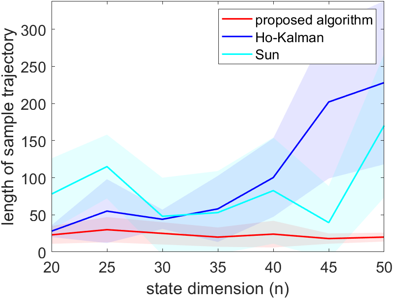
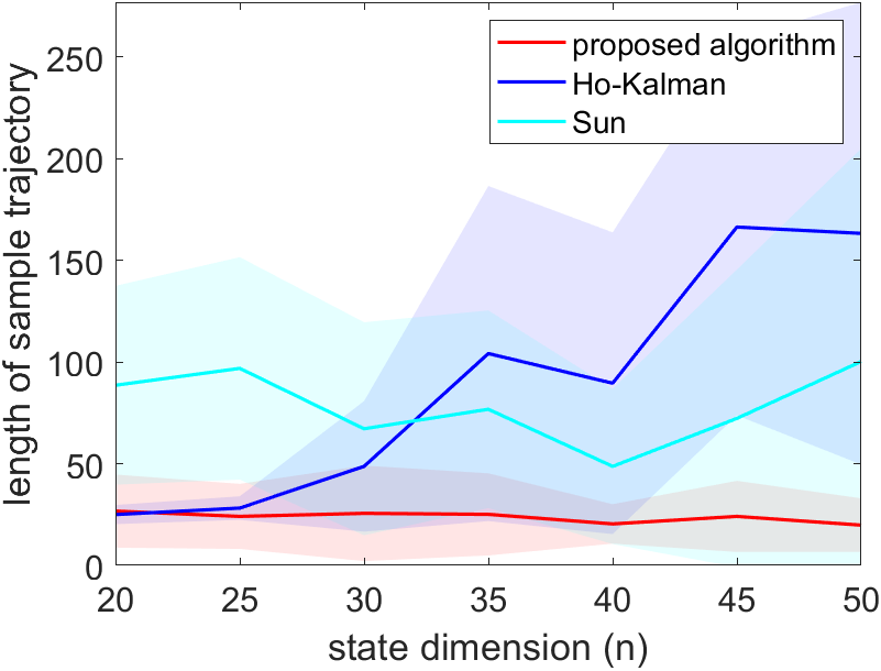
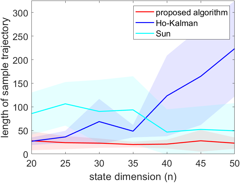
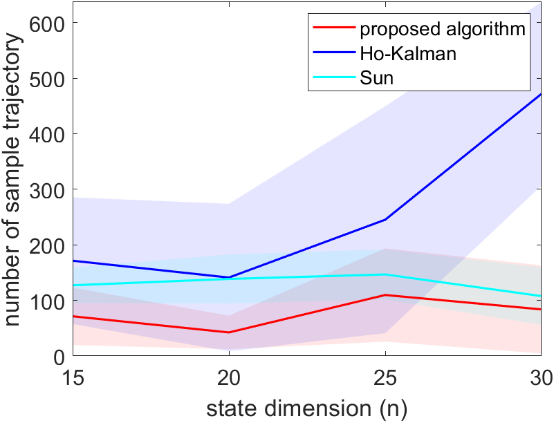
In the first part of the simulations, we fix the number of rollouts to be 44 times the dimension of the system and let the system run with an increasing length of rollouts until a stabilizing controller is generated. The system is simulated in three different settings, each with noise wt,vt𝒩(0,σ)w_{t},v_{t}\sim\mathcal{N}(0,\sigma), with σ=0.4,0.6,0.8\sigma=0.4,0.6,0.8. For each of the three algorithms, the simulation is repeated for 30 trails, and the result is shown in Figure 1. The proposed method requires the shortest rollouts. The algorithm in Sun et al. [2020] roughly have the same length of rollouts across different dimensions. This is to be expected, as Sun et al. [2020] only uses the last data point of each rollout, so a longer trajectory does not generate more data. However, unlike the proposed algorithm, Sun et al. [2020] still needs to estimate the entire system, which is why it still needs a longer rollout. The length of the rollouts of Zheng and Li [2020] grows linearly with the dimension of the system. We also see fluctuations of the length of rollouts required for stabilization in Figure 1 because the matrix generated for each nn has a randomly generated eigenbasis, which influences the amount of data needed for stabilization, as shown in Theorem 5.3. Overall, this simulation shows that the length of rollouts of the proposed algorithm remains O(poly(k))O(\text{poly}(k)) regardless of the dimension of the system nn.

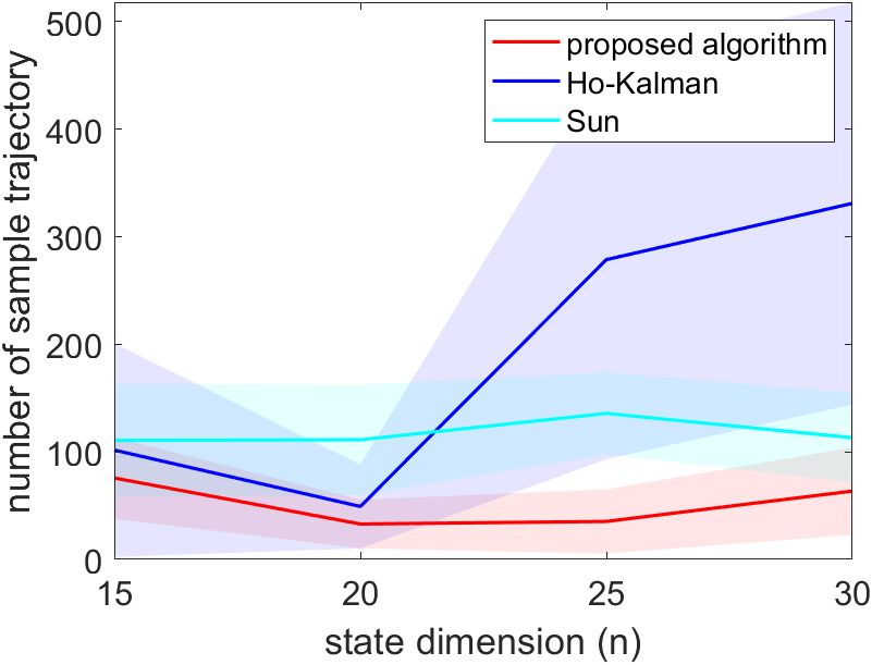
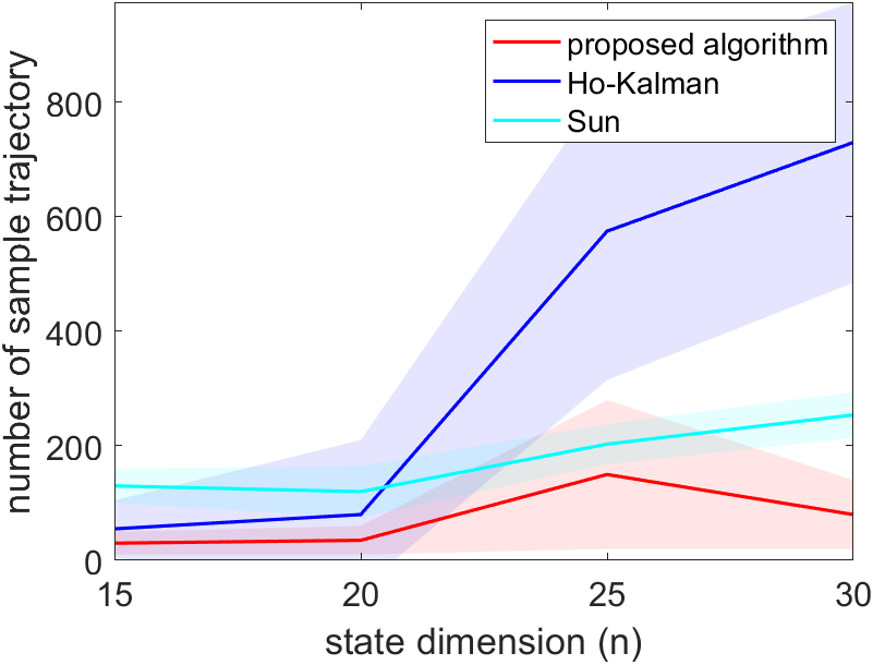
In the second part of the simulation, we fix the length of each trajectory to 7070 and examine the number of trajectories needed before the system stabilizes. We do not increase the length of trajectory in this part of the simulation with increasing nn, since Sun et al. [2020] only uses the last data point, and does not show significant performance improvement with longer trajectories, as shown in the first part of the simulation, so it would be an unfair comparison if the trajectory is overly long. Similar to the first part, the system is simulated in three different settings and the result is shown in Figure 2. Overall, the proposed method requires the least number of trajectories. When the nkn\gtrapprox k, the proposed algorithm requires a similar number of data with Zheng and Li [2020], as the proposed algorithm is the same to that in Zheng and Li [2020] when k=nk=n. When nkn\gg k, the proposed algorithm out-performs both benchmarks.

References

  • Abbasi-Yadkori and Szepesvári [2011] Y. Abbasi-Yadkori and C. Szepesvári. Regret bounds for the adaptive control of linear quadratic systems. In S. M. Kakade and U. von Luxburg, editors, Proceedings of the 24th Annual Conference on Learning Theory, volume 19 of Proceedings of Machine Learning Research, pages 1–26, Budapest, Hungary, 09–11 Jun 2011. PMLR.
  • Ahlfors [1966] L. V. Ahlfors. Complex Analysis. McGraw-Hill Book Company, 2 edition, 1966.
  • Beard et al. [1997] R. W. Beard, G. N. Saridis, and J. T. Wen. Galerkin approximations of the generalized hamilton-jacobi-bellman equation. Automatica, 33(12):2159–2177, 1997. ISSN 0005-1098. doi: https://doi.org/10.1016/S0005-1098(97)00128-3.
  • Berberich et al. [2020] J. Berberich, J. Köhler, M. Muller, and F. Allgöwer. Data-driven model predictive control with stability and robustness guarantees. IEEE Transactions on Automatic Control, PP:1–1, 06 2020. doi: 10.1109/TAC.2020.3000182.
  • Bouazza et al. [2021] L. Bouazza, B. Mourllion, A. Makhlouf, and A. Birouche. Controllability and observability of formal perturbed linear time invariant systems. International Journal of Dynamics and Control, 9, 12 2021. doi: 10.1007/s40435-021-00786-4.
  • Bradtke et al. [1994] S. Bradtke, B. Ydstie, and A. Barto. Adaptive linear quadratic control using policy iteration. Proceedings of the American Control Conference, 3, 09 1994. doi: 10.1109/ACC.1994.735224.
  • Chen and Zhang [1989] H.-F. Chen and J.-F. Zhang. Convergence rates in stochastic adaptive tracking. International Journal of Control, 49(6):1915–1935, 1989. doi: 10.1080/00207178908559752.
  • Chen and Astolfi [2021] K. Chen and A. Astolfi. Adaptive control for systems with time-varying parameters. IEEE Transactions on Automatic Control, 66(5):1986–2001, 2021. doi: 10.1109/TAC.2020.3046141.
  • Chen and Hazan [2020] X. Chen and E. Hazan. Black-box control for linear dynamical systems. CoRR, abs/2007.06650, 2020.
  • Cohen et al. [2019] A. Cohen, T. Koren, and Y. Mansour. Learning linear-quadratic regulators efficiently with only T\sqrt{T} regret. In K. Chaudhuri and R. Salakhutdinov, editors, Proceedings of the 36th International Conference on Machine Learning, volume 97 of Proceedings of Machine Learning Research, pages 1300–1309. PMLR, 09–15 Jun 2019.
  • De Persis and Tesi [2020] C. De Persis and P. Tesi. Formulas for data-driven control: Stabilization, optimality, and robustness. IEEE Transactions on Automatic Control, 65(3):909–924, 2020. doi: 10.1109/TAC.2019.2959924.
  • Dean S. Mania [2020] N. e. a. Dean S. Mania, H. Matni. On the sample complexity of the linear quadratic regulator. Foundations of Computational Mathematics, 20:633–679, 2020. doi: https://doi.org/10.1007/s10208-019-09426-y.
  • Dullerud and Paganini [2000] G. E. Dullerud and F. Paganini. A Course in Robust Control Theory. Springer, New York, NY, 2000.
  • Faradonbeh [2017] M. K. S. Faradonbeh. Non-Asymptotic Adaptive Control of Linear-Quadratic Systems. PhD thesis, University of Michigan, 2017.
  • Fattahi [2021] S. Fattahi. Learning partially observed linear dynamical systems from logarithmic number of samples. In A. Jadbabaie, J. Lygeros, G. J. Pappas, P. A. Parrilo, B. Recht, C. J. Tomlin, and M. N. Zeilinger, editors, Proceedings of the 3rd Conference on Learning for Dynamics and Control, volume 144 of Proceedings of Machine Learning Research, pages 60–72. PMLR, 07 – 08 June 2021.
  • Fazel et al. [2019] M. Fazel, R. Ge, S. M. Kakade, and M. Mesbahi. Global convergence of policy gradient methods for the linear quadratic regulator, 2019.
  • Horn and Johnson [1985] R. A. Horn and C. R. Johnson. Matrix Analysis. Cambridge University Press, 1985.
  • Horn and Johnson [2012] R. A. Horn and C. R. Johnson. Matrix Analysis. Cambridge University Press, USA, 2nd edition, 2012. ISBN 0521548233.
  • Hu et al. [2022] Y. Hu, A. Wierman, and G. Qu. On the sample complexity of stabilizing lti systems on a single trajectory. In Neurips, pages 1–2, 2022. doi: 10.1109/Allerton49937.2022.9929403.
  • Ibrahimi et al. [2012] M. Ibrahimi, A. Javanmard, and B. V. Roy. Efficient reinforcement learning for high dimensional linear quadratic systems. In Neural Information Processing Systems, 2012.
  • Jansch-Porto et al. [2020] J. P. Jansch-Porto, B. Hu, and G. E. Dullerud. Policy learning of mdps with mixed continuous/discrete variables: A case study on model-free control of markovian jump systems. CoRR, abs/2006.03116, 2020. URL https://arxiv.org/abs/2006.03116.
  • Jiang and Wang [2002] Z.-P. Jiang and Y. Wang. A converse lyapunov theorem for discrete-time systems with disturbances. Systems & Control Letters, 45(1):49–58, 2002. ISSN 0167-6911. doi: https://doi.org/10.1016/S0167-6911(01)00164-5.
  • Krauth et al. [2019] K. Krauth, S. Tu, and B. Recht. Finite-time analysis of approximate policy iteration for the linear quadratic regulator. Advances in Neural Information Processing Systems, 32, 2019.
  • Kusii [2018] S. Kusii. Stabilization and attenuation of bounded perturbations in discrete control systems. Journal of Mathematical Sciences, 2018. doi: https://doi.org/10.1007/s10958-018-3848-3.
  • Lai [1986] T. Lai. Asymptotically efficient adaptive control in stochastic regression models. Advances in Applied Mathematics, 7(1):23–45, 1986. ISSN 0196-8858. doi: https://doi.org/10.1016/0196-8858(86)90004-7.
  • Lai and Ying [1991] T. L. Lai and Z. Ying. Parallel recursive algorithms in asymptotically efficient 496 adaptive control of linear stochastic systems. SIAM Journal on Control and Optimization, 29(5):1091–1127, 1991.
  • Lale et al. [2020] S. Lale, K. Azizzadenesheli, B. Hassibi, and A. Anandkumar. Explore more and improve regret in linear quadratic regulators. CoRR, abs/2007.12291, 2020. URL https://arxiv.org/abs/2007.12291.
  • Lee et al. [2023] B. D. Lee, A. Rantzer, and N. Matni. Nonasymptotic regret analysis of adaptive linear quadratic control with model misspecification, 2023.
  • Li et al. [2022] Y. Li, Y. Tang, R. Zhang, and N. Li. Distributed reinforcement learning for decentralized linear quadratic control: A derivative-free policy optimization approach. IEEE Transactions on Automatic Control, 67(12):6429–6444, 2022. doi: 10.1109/TAC.2021.3128592.
  • Liu et al. [2023] W. Liu, Y. Li, J. Sun, G. Wang, and J. Chen. Robust control of unknown switched linear systems from noisy data. ArXiv, abs/2311.11300, 2023.
  • Mania et al. [2019] H. Mania, S. Tu, and B. Recht. Certainty equivalence is efficient for linear quadratic control. Proceedings of the 33rd International Conference on Neural Information Processing Systems, 2019.
  • Oymak and Ozay [2018a] S. Oymak and N. Ozay. Non-asymptotic identification of lti systems from a single trajectory. 2019 American Control Conference (ACC), pages 5655–5661, 2018a.
  • Oymak and Ozay [2018b] S. Oymak and N. Ozay. Non-asymptotic identification of lti systems from a single trajectory. 2019 American Control Conference (ACC), pages 5655–5661, 2018b. URL https://api.semanticscholar.org/CorpusID:49275079.
  • Pasik-Duncan [1996] B. Pasik-Duncan. Adaptive control [second edition, by karl j. astrom and bjorn wittenmark, addison wesley (1995)]. IEEE Control Systems Magazine, 16(2):87–, 1996.
  • Perdomo et al. [2021] J. C. Perdomo, J. Umenberger, and M. Simchowitz. Stabilizing dynamical systems via policy gradient methods. ArXiv, abs/2110.06418, 2021.
  • Petros A. Ioannou [2001] J. S. Petros A. Ioannou. Robust adaptive control. Autom., 37(5):793–795, 2001.
  • Plevrakis and Hazan [2020] O. Plevrakis and E. Hazan. Geometric exploration for online control. In Proceedings of the 34th International Conference on Neural Information Processing Systems, NIPS’20, Red Hook, NY, USA, 2020. Curran Associates Inc. ISBN 9781713829546.
  • Sarkar and Rakhlin [2018] T. Sarkar and A. Rakhlin. Near optimal finite time identification of arbitrary linear dynamical systems. In International Conference on Machine Learning, 2018.
  • Sarkar et al. [2019] T. Sarkar, A. Rakhlin, and M. A. Dahleh. Finite-time system identification for partially observed lti systems of unknown order. ArXiv, abs/1902.01848, 2019.
  • Simchowitz et al. [2018] M. Simchowitz, H. Mania, S. Tu, M. I. Jordan, and B. Recht. Learning without mixing: Towards a sharp analysis of linear system identification. Annual Conference Computational Learning Theory, 2018.
  • Sun et al. [2020] Y. Sun, S. Oymak, and M. Fazel. Finite sample system identification: Optimal rates and the role of regularization. In A. M. Bayen, A. Jadbabaie, G. Pappas, P. A. Parrilo, B. Recht, C. Tomlin, and M. Zeilinger, editors, Proceedings of the 2nd Conference on Learning for Dynamics and Control, volume 120 of Proceedings of Machine Learning Research, pages 16–25. PMLR, 10–11 Jun 2020.
  • Tsiamis and Pappas [2021] A. Tsiamis and G. J. Pappas. Linear systems can be hard to learn. In 2021 60th IEEE Conference on Decision and Control (CDC), pages 2903–2910, 2021. doi: 10.1109/CDC45484.2021.9682778.
  • Tu and Recht [2018] S. Tu and B. Recht. The gap between model-based and model-free methods on the linear quadratic regulator: An asymptotic viewpoint. In Annual Conference Computational Learning Theory, 2018.
  • Wang et al. [2022] W. Wang, X. Xie, and C. Feng. Model-free finite-horizon optimal tracking control of discrete-time linear systems. Appl. Math. Comput., 433(C), nov 2022. ISSN 0096-3003. doi: 10.1016/j.amc.2022.127400.
  • Xing et al. [2022] Y. Xing, B. Gravell, X. He, K. H. Johansson, and T. H. Summers. Identification of linear systems with multiplicative noise from multiple trajectory data. Automatica, 144:110486, 2022. ISSN 0005-1098. doi: https://doi.org/10.1016/j.automatica.2022.110486.
  • Zeng et al. [2023] X. Zeng, Z. Liu, Z. Du, N. Ozay, and M. Sznaier. On the hardness of learning to stabilize linear systems. 2023 62nd IEEE Conference on Decision and Control (CDC), pages 6622–6628, 2023.
  • Zhang et al. [2020] K. Zhang, B. Hu, and T. Basar. Policy optimization for 2\mathcal{H}_{2} linear control with \mathcal{H}_{\infty} robustness guarantee: Implicit regularization and global convergence. In A. M. Bayen, A. Jadbabaie, G. Pappas, P. A. Parrilo, B. Recht, C. Tomlin, and M. Zeilinger, editors, Proceedings of the 2nd Conference on Learning for Dynamics and Control, volume 120 of Proceedings of Machine Learning Research, pages 179–190. PMLR, 10–11 Jun 2020.
  • Zhang et al. [2024] Z. Zhang, Y. Nakahira, and G. Qu. Learning to stabilize unknown lti systems on a single trajectory under stochastic noise, 2024.
  • Zheng and Li [2020] Y. Zheng and N. Li. Non-asymptotic identification of linear dynamical systems using multiple trajectories. IEEE Control Systems Letters, PP:1–1, 12 2020. doi: 10.1109/LCSYS.2020.3042924.
  • Zheng et al. [2020] Y. Zheng, L. Furieri, M. Kamgarpour, and N. Li. Sample complexity of linear quadratic gaussian (lqg) control for output feedback systems. Conference on Learning for Dynamics & Control, 2020.
  • Zhou and Doyle [1998] K. Zhou and J. C. Doyle. Essentials of Robust Control. Prentice-Hall, 1998.

Appendix A Proof of Step 1: Bounding Hankel Matrix Error

To further simplify notation, define

Y\displaystyle Y =[y(1)y(M)],\displaystyle=\begin{bmatrix}y^{(1)}&\dots&y^{(M)}\end{bmatrix}, (46)
U\displaystyle U =[U(1)U(M)],\displaystyle=\begin{bmatrix}U^{(1)}&\dots&U^{(M)}\end{bmatrix}, (47)
v\displaystyle v =[v(1)v(M)],\displaystyle=\begin{bmatrix}v^{(1)}&\dots&v^{(M)}\end{bmatrix}, (48)

so (36) can be simplified to

Φ^\displaystyle\hat{\Phi} =argminXdy×(Tdu)YXUF2,\displaystyle=\arg\min_{X\in\mathbb{R}^{d_{y}\times(T*d_{u})}}\left\|Y-XU\right\|_{F}^{2}, (49)

respectively. An analytic solution to (49) is Φ^:=YU\hat{\Phi}:=YU^{{\dagger}}, where U:=U(UU)1U^{{\dagger}}:=U^{*}(UU^{*})^{-1} is the right psuedo-inverse of UU. In this paper, we will use Φ~^\hat{\tilde{\Phi}} to recover H~\tilde{H}, and we want to bound the error between H~\tilde{H} and H~^\hat{\tilde{H}}.

Φ^Φ=YU(UU)1Φ=(YΦU)U(UU)1=vU(UU)1,\begin{split}\hat{\Phi}-\Phi&=YU^{*}(UU^{*})^{-1}-\Phi\\ &=(Y-\Phi U)U^{*}(UU^{*})^{-1}\\ &=vU^{*}(UU^{*})^{-1},\end{split} (50)

where the third equality used (35). We can bound the estimation error (50) by

Φ^Φ(UU)1vU.\left\|\hat{\Phi}-\Phi\right\|\leq\left\|(UU^{*})^{-1}\right\|\left\|vU^{*}\right\|. (51)

We then prove a lemma that links the difference between Φ\Phi and Hankel matrix HH.

Lemma A.1.

Given two Hankel matrices H,HH^{\clubsuit},H^{\diamondsuit} constructed from Φ,Φ\Phi^{\clubsuit},\Phi^{\diamondsuit} with (37), respectively, then

HHmin{p,q}Φ2+m:TΦ2+m:T.\left\|H^{\clubsuit}-H^{\diamondsuit}\right\|\leq\sqrt{\min\{p,q\}}\left\|\Phi_{2+m:T}^{\clubsuit}-\Phi_{2+m:T}^{\diamondsuit}\right\|.
Proof.

From the construction in (37), we see that each column of HHH^{\clubsuit}-H^{\diamondsuit} is a submatrix of Φ2+m:TΦ2+m:T\Phi_{2+m:T}^{\clubsuit}-\Phi_{2+m:T}^{\diamondsuit}, then

HHqΦ2+m:TΦ2+m:T.\left\|H^{\clubsuit}-H^{\diamondsuit}\right\|\leq\sqrt{q}\left\|\Phi_{2+m:T}^{\clubsuit}-\Phi_{2+m:T}^{\diamondsuit}\right\|. (52)

Similarly, each row of HHH^{\clubsuit}-H^{\diamondsuit} is a submatrix of Φ2+m:TΦ2+m:T\Phi_{2+m:T}^{\clubsuit}-\Phi_{2+m:T}^{\diamondsuit}. Therefore,

HHpΦ2+m:TΦ2+m:T.\left\|H^{\clubsuit}-H^{\diamondsuit}\right\|\leq\sqrt{p}\left\|\Phi_{2+m:T}^{\clubsuit}-\Phi_{2+m:T}^{\diamondsuit}\right\|. (53)

Combining (52) and (53) gives the desired result. ∎

We then bound the gap between H(k)H^{(k)} and H~^\hat{\tilde{H}} by adapting Theorem 3.1 of Zheng and Li [2020]. For completeness, we put the theorem and proof below:

Theorem A.2.

For any δ>0\delta>0, the following inequality holds when M>8duT+4(du+dy+4)log(3T/δ)M>8d_{u}T+4(d_{u}+d_{y}+4)\log(3T/\delta) with probability at least 1δ1-\delta:

HH^8σvT(T+1)(du+dy)min{p,q}log(27T/δ)σuM:=ϵ^\left\|H-\hat{H}\right\|\leq\frac{8\sigma_{v}\sqrt{T(T+1)(d_{u}+d_{y})\min\{p,q\}\log(27T/\delta)}}{\sigma_{u}\sqrt{M}}:=\hat{\epsilon}
Proof.

By Lemma A.1, we have

HH^min{p,q}Φ2+m:TΦ^2+m:T.\left\|H-\hat{H}\right\|\leq\sqrt{\min\{p,q\}}\left\|\Phi_{2+m:T}-\hat{\Phi}_{2+m:T}\right\|.

Bounding (UU)1\left\|(UU^{*})\right\|^{-1} and vU\left\|vU^{*}\right\| with Proposition 3.1 and Proposition 3.2 of Zheng and Li [2020] gives the result in the theorem statement. ∎

Lemma A.3.
HH~qpL3(|λk+1|+12)m:=ϵ~\left\|H-\tilde{H}\right\|\leq\sqrt{q}p\leq L^{3}(\frac{|\lambda_{k+1}|+1}{2})^{m}:=\tilde{\epsilon}
Proof.

We first bound HH and H~\tilde{H} entry-wise,

Hi,jH~i,j=\displaystyle H_{i,j}-\tilde{H}_{i,j}= CAm+i+j2BCQ1N1m+i+j2R1B\displaystyle CA^{m+i+j-2}B-CQ_{1}N_{1}^{m+i+j-2}R_{1}B
=\displaystyle= C(Q1N1m+i+j2R1+Q2N2m+i+j2R2)BCQ1N1m+i+j2R1B\displaystyle C(Q_{1}N_{1}^{m+i+j-2}R_{1}+Q_{2}N_{2}^{m+i+j-2}R_{2})B-CQ_{1}N_{1}^{m+i+j-2}R_{1}B
=\displaystyle= CQ2N2m+i+j2R2B.\displaystyle CQ_{2}N_{2}^{m+i+j-2}R_{2}B.

Applying Gelfand’s formula (Lemma F.2), we obtain

Hi,jH~i,jBCζϵ2(N2)(|λk+1|+ϵ4)m+i+j2L3(|λk+1|+12)m+i+j2.\left\|H_{i,j}-\tilde{H}_{i,j}\right\|\leq\left\|B\right\|\left\|C\right\|\zeta_{\epsilon_{2}}(N_{2})(|\lambda_{k+1}|+\epsilon_{4})^{m+i+j-2}\leq L^{3}(\frac{|\lambda_{k+1}|+1}{2})^{m+i+j-2}. (54)

Moreover, we have the following well-known inequality (see, for example, Horn and Johnson [1985]), for Λn1×n2\Lambda\in\mathbb{R}^{n_{1}\times n_{2}},

1n1Λ1Λ2n2Λ1.\frac{1}{\sqrt{n_{1}}}\left\|\Lambda\right\|_{1}\leq\left\|\Lambda\right\|_{2}\leq\sqrt{n_{2}}\left\|\Lambda\right\|_{1}. (55)

Applying (55) to (54) gives us the desired inequality. ∎

We are now ready to prove Lemma 6.1.

Proof of Lemma 6.1.

We first provide a bound on H~^H^\hat{\tilde{H}}-\hat{H}. As H~^\hat{\tilde{H}} is the rank-kk approximation of H^\hat{H}, we have H~^H^H~H^\left\|\hat{\tilde{H}}-\hat{H}\right\|\leq\left\|\tilde{H}-\hat{H}\right\|, then

H~^H^H~H+HH^=ϵ~+ϵ^.\left\|\hat{\tilde{H}}-\hat{H}\right\|\leq\left\|\tilde{H}-H\right\|+\left\|H-\hat{H}\right\|=\tilde{\epsilon}+\hat{\epsilon}. (56)

where we use Theorem A.2 and Lemma A.3. Therefore, we obtain the following bound

H~^H~H~^H^+H^H+HH~2ϵ^+2ϵ~:=ϵ.\left\|\hat{\tilde{H}}-\tilde{H}\right\|\leq\left\|\hat{\tilde{H}}-\hat{H}\right\|+\left\|\hat{H}-H\right\|+\left\|H-\tilde{H}\right\|\leq 2\hat{\epsilon}+2\tilde{\epsilon}:=\epsilon. (57)

Appendix B Proof of Step 2: Bounding Dynamics Error

In the previous section, we proved Lemma 6.1 and provided a bound for H~^H~\|\hat{\tilde{H}}-\tilde{H}\|. In this section, we use this bound to derive the error bound for our system estimation. We start with the following lemma that bounds the difference between 𝒪~\tilde{\mathbf{\mathcal{O}}} and 𝒪^\hat{\mathbf{\mathcal{O}}} and the difference between 𝒞~\tilde{\mathbf{\mathcal{C}}} and 𝒞^\hat{\mathbf{\mathcal{C}}} up to a transformation.

Lemma B.1.

Given N1N_{1} is diagnalizable, and recall N1=P1ΛP11N_{1}=P_{1}\Lambda P_{1}^{-1} denotes the eigenvalue decomposition of N1N_{1}, where Λ=diag(λ1,,λk)\Lambda=\operatorname{diag}(\lambda_{1},\dots,\lambda_{k}) is the diagonal matrix of eigenvalues. Consider H~^=𝒪^𝒞^\hat{\tilde{H}}=\hat{\mathbf{\mathcal{O}}}\hat{\mathbf{\mathcal{C}}} and H~=𝒪~𝒞~\tilde{H}=\tilde{\mathbf{\mathcal{O}}}\tilde{\mathbf{\mathcal{C}}}, where we recall 𝒪^,𝒞^\hat{\mathbf{\mathcal{O}}},\hat{\mathbf{\mathcal{C}}} are obtained by doing SVD H~^=U^Σ^V^\hat{\tilde{H}}=\hat{U}\hat{\Sigma}\hat{V}^{*} and setting 𝒪^=U^Σ^1/2,𝒞^=Σ^1/2V^\hat{\mathbf{\mathcal{O}}}=\hat{U}\hat{\Sigma}^{1/2},\hat{\mathbf{\mathcal{C}}}=\hat{\Sigma}^{1/2}\hat{V}^{*} (cf. (39)). Suppose ΔH=H~H~^ϵ\left\|\Delta_{H}\right\|=\left\|\tilde{H}-\hat{\tilde{H}}\right\|\leq\epsilon, then there exists an invertible kk-by-kk matrix S^\hat{S} such that

  1. (a)

    𝒪~𝒪^S^1σmin(𝒞~)ϵ\left\|\tilde{\mathbf{\mathcal{O}}}-\hat{\mathbf{\mathcal{O}}}\hat{S}\right\|\leq\frac{1}{\sigma_{\min}(\tilde{\mathbf{\mathcal{C}}})}\epsilon and 𝒞~S^1𝒞^4σmin(𝒪~)ϵ\left\|\tilde{\mathbf{\mathcal{C}}}-\hat{S}^{-1}\hat{\mathbf{\mathcal{C}}}\right\|\leq\frac{4}{\sigma_{\min}(\tilde{\mathbf{\mathcal{O}}})}\epsilon,

  2. (b)

    there exists c1,c2>0c_{1},c_{2}>0 such that c1IS^c2Ic_{1}I\preceq\hat{S}\preceq c_{2}I, where given σ¯s,σ¯s\underline{\sigma}_{s},\overline{\sigma}_{s} in (68),

    c12=σ¯s22σmax(P1)2,c22=22σ¯sσmin(P1)2.c_{1}^{2}=\frac{\underline{\sigma}_{s}}{2\sqrt{2}\sigma_{\max}(P_{1})^{2}},\qquad c_{2}^{2}=2\sqrt{2}\frac{\overline{\sigma}_{s}}{\sigma_{\min}(P_{1})^{2}}.
  3. (c)

    we can bound σmin(𝒪~)\sigma_{\min}(\tilde{\mathbf{\mathcal{O}}}) and σmin(𝒞~)\sigma_{\min}(\tilde{\mathbf{\mathcal{C}}}) as follows:

    σmin(𝒪~)\displaystyle\sigma_{\min}(\tilde{\mathbf{\mathcal{O}}}) σmin(𝒪~1:α)σmin(𝒢ob)σmin(N1m/2):=o~min(m),\displaystyle\geq\sigma_{\min}(\tilde{\mathbf{\mathcal{O}}}_{1:\alpha})\geq\sigma_{\min}(\mathcal{G}_{\mathrm{ob}})\sigma_{\min}(N_{1}^{m/2}):=\tilde{o}_{\min}(m),
    σmin(𝒞~)\displaystyle\sigma_{\min}(\tilde{\mathbf{\mathcal{C}}}) σmin(𝒞~1:α)σmin(𝒢con)σmin(N1m/2):=c~min(m).\displaystyle\geq\sigma_{\min}(\tilde{\mathbf{\mathcal{C}}}_{1:\alpha})\geq\sigma_{\min}(\mathcal{G}_{\mathrm{con}})\sigma_{\min}(N_{1}^{m/2}):=\tilde{c}_{\min}(m).
Proof.

Proof of part(a). Recall the definition of H~\tilde{H}

H~=\displaystyle\tilde{H}= [CQ1N1m+i+jR1B]i{0,,p1},j{0,,q1}\displaystyle[CQ_{1}N_{1}^{m+i+j}R_{1}B]_{i\in\{0,\dots,p-1\},j\in\{0,\dots,q-1\}}
=\displaystyle= [CQ1N1m2CQ1N1m2+p1]𝒪~[N1m2R1BN1m2+q1R1B]𝒞~.\displaystyle\underbrace{\begin{bmatrix}CQ_{1}N_{1}^{\frac{m}{2}}\\ \ldots\\ CQ_{1}N_{1}^{\frac{m}{2}+p-1}\end{bmatrix}}_{\tilde{\mathbf{\mathcal{O}}}}\underbrace{\begin{bmatrix}N_{1}^{\frac{m}{2}}R_{1}B&\dots&N_{1}^{\frac{m}{2}+q-1}R_{1}B\end{bmatrix}}_{\tilde{\mathbf{\mathcal{C}}}}.

We can represent 𝒪~\tilde{\mathbf{\mathcal{O}}} and 𝒞~\tilde{\mathbf{\mathcal{C}}} as follows:

𝒪~=[CQ1P1CQ1P1CQ1P1][Λm2Λm2+p1]:=G1P11.\tilde{\mathbf{\mathcal{O}}}=\underbrace{\begin{bmatrix}CQ_{1}P_{1}&&&\\ &CQ_{1}P_{1}&&\\ &&\dots&\\ &&&CQ_{1}P_{1}\end{bmatrix}\begin{bmatrix}\Lambda^{\frac{m}{2}}\\ \ldots\\ \Lambda^{\frac{m}{2}+p-1}\end{bmatrix}}_{:=G_{1}}P_{1}^{-1}. (58)
𝒞~=P1[Λm2Λm2+q1][P11R1BP11R1B]:=G2.\tilde{\mathbf{\mathcal{C}}}=P_{1}\underbrace{\begin{bmatrix}\Lambda^{\frac{m}{2}}&\dots&\Lambda^{\frac{m}{2}+q-1}\end{bmatrix}\begin{bmatrix}P_{1}^{-1}R_{1}B&&\\ &\dots&\\ &&P_{1}^{-1}R_{1}B\end{bmatrix}}_{:=G_{2}^{*}}. (59)

Next, note that

H~^=\displaystyle\hat{\tilde{H}}= U^Σ^V^=U^Σ^12Σ^12V^=𝒪^𝒞^=𝒪~𝒞~+ΔH=G1G2+ΔH.\displaystyle\hat{U}\hat{\Sigma}\hat{V}^{*}=\hat{U}\hat{\Sigma}^{\frac{1}{2}}\hat{\Sigma}^{\frac{1}{2}}\hat{V}^{*}=\hat{\mathbf{\mathcal{O}}}\hat{\mathbf{\mathcal{C}}}=\tilde{\mathbf{\mathcal{O}}}\tilde{\mathbf{\mathcal{C}}}+\Delta_{H}=G_{1}G_{2}^{*}+\Delta_{H}. (60)

Therefore, we have

G1G2G2=U^Σ^12𝒪^Σ^12V^G2ΔHG2G1=𝒪^Σ^12V^G2(G2G2)1ΔHG2(G2G2)1𝒪~=G1P11=𝒪^Σ^12V^G2(G2G2)1P11:=S^ΔHG2(G2G2)1P11.\begin{split}&G_{1}G_{2}^{*}G_{2}=\underbrace{\hat{U}\hat{\Sigma}^{\frac{1}{2}}}_{\hat{\mathbf{\mathcal{O}}}}\hat{\Sigma}^{\frac{1}{2}}\hat{V}^{*}G_{2}-\Delta_{H}G_{2}\\ \Rightarrow&G_{1}=\hat{\mathbf{\mathcal{O}}}\hat{\Sigma}^{\frac{1}{2}}\hat{V}^{*}G_{2}(G_{2}^{*}G_{2})^{-1}-\Delta_{H}G_{2}(G_{2}^{*}G_{2})^{-1}\\ \Rightarrow&\tilde{\mathbf{\mathcal{O}}}=G_{1}P_{1}^{-1}=\hat{\mathbf{\mathcal{O}}}\underbrace{\hat{\Sigma}^{\frac{1}{2}}\hat{V}^{*}G_{2}(G_{2}^{*}G_{2})^{-1}P_{1}^{-1}}_{:=\hat{S}}-\Delta_{H}G_{2}(G_{2}^{*}G_{2})^{-1}P_{1}^{-1}.\end{split} (61)

where we have defined the matrix S^\hat{S} above. We can also expand S^\hat{S} as follows:

S^\displaystyle\hat{S} =Σ^12V^G2P1(P1)1(G2G2)1P11\displaystyle=\hat{\Sigma}^{\frac{1}{2}}\hat{V}^{*}G_{2}P_{1}^{*}(P_{1}^{*})^{-1}(G_{2}^{*}G_{2})^{-1}P_{1}^{-1}
=Σ^12V^G2P1(P1G2G2P1)1\displaystyle=\hat{\Sigma}^{\frac{1}{2}}\hat{V}^{*}G_{2}P_{1}^{*}(P_{1}G_{2}^{*}G_{2}P_{1}^{*})^{-1}
=𝒞^𝒞~(𝒞~𝒞~)1.\displaystyle=\hat{\mathbf{\mathcal{C}}}\tilde{\mathbf{\mathcal{C}}}^{*}(\tilde{\mathbf{\mathcal{C}}}\tilde{\mathbf{\mathcal{C}}}^{*})^{-1}. (62)

Further, the last term in the last equation in (61) can be written as,

ΔHG2(G2G2)1P11\displaystyle\Delta_{H}G_{2}(G_{2}^{*}G_{2})^{-1}P_{1}^{-1} =ΔHG2P1(P1)1(G2G2)1P11\displaystyle=\Delta_{H}G_{2}P_{1}^{*}(P_{1}^{*})^{-1}(G_{2}^{*}G_{2})^{-1}P_{1}^{-1}
=ΔH𝒞~(𝒞~𝒞~)1.\displaystyle=\Delta_{H}\tilde{\mathbf{\mathcal{C}}}^{*}(\tilde{\mathbf{\mathcal{C}}}\tilde{\mathbf{\mathcal{C}}}^{*})^{-1}. (63)

Putting (61), (63) together, we have

𝒪~𝒪^S^1σmin(𝒞~)ϵ,\left\|\tilde{\mathbf{\mathcal{O}}}-\hat{\mathbf{\mathcal{O}}}\hat{S}\right\|\leq\frac{1}{\sigma_{\min}(\tilde{\mathbf{\mathcal{C}}})}\epsilon, (64)

which proves one side of part (a). To finish part(a), we are left to bound 𝒞~S^1𝒞^\left\|\tilde{\mathbf{\mathcal{C}}}-\hat{S}^{-1}\hat{\mathbf{\mathcal{C}}}\right\|. With the expression of S^\hat{S} in (62), we obtain

𝒞^S^1𝒞~=𝒞^𝒞~𝒞~(𝒞^𝒞~)1𝒞~.\left\|\hat{\mathbf{\mathcal{C}}}-\hat{S}^{-1}\tilde{\mathbf{\mathcal{C}}}\right\|=\left\|\hat{\mathbf{\mathcal{C}}}-\tilde{\mathbf{\mathcal{C}}}\tilde{\mathbf{\mathcal{C}}}^{*}(\hat{\mathbf{\mathcal{C}}}\tilde{\mathbf{\mathcal{C}}}^{*})^{-1}\tilde{\mathbf{\mathcal{C}}}\right\|.

Let E:=𝒪^S^𝒪~E:=\hat{\mathbf{\mathcal{O}}}\hat{S}-\tilde{\mathbf{\mathcal{O}}} so 𝒪~=𝒪^S^E\tilde{\mathbf{\mathcal{O}}}=\hat{\mathbf{\mathcal{O}}}\hat{S}-E. By (61) and (63), we obtain

E=ΔH𝒞~(𝒞~𝒞~)1,E=\Delta_{H}\tilde{\mathbf{\mathcal{C}}}^{*}(\tilde{\mathbf{\mathcal{C}}}\tilde{\mathbf{\mathcal{C}}}^{*})^{-1}, (65)

and

E𝒞~=ΔH𝒞~(𝒞~𝒞~)1𝒞~ϵ.\left\|E\tilde{\mathbf{\mathcal{C}}}\right\|=\left\|\Delta_{H}\tilde{\mathbf{\mathcal{C}}}^{*}(\tilde{\mathbf{\mathcal{C}}}\tilde{\mathbf{\mathcal{C}}}^{*})^{-1}\tilde{\mathbf{\mathcal{C}}}\right\|\leq\epsilon.

Therefore, we can obtain the following inequalities:

ϵ𝒪~𝒞~𝒪^𝒞^=(𝒪^S^E)𝒞~𝒪^𝒞^=𝒪^(S^𝒞~𝒞^)E𝒞~𝒪^(S^𝒞~𝒞^)E𝒞~\displaystyle\epsilon\geq\left\|\tilde{\mathbf{\mathcal{O}}}\tilde{\mathbf{\mathcal{C}}}-\hat{\mathbf{\mathcal{O}}}\hat{\mathbf{\mathcal{C}}}\right\|=\left\|(\hat{\mathbf{\mathcal{O}}}\hat{S}-E)\tilde{\mathbf{\mathcal{C}}}-\hat{\mathbf{\mathcal{O}}}\hat{\mathbf{\mathcal{C}}}\right\|=\left\|\hat{\mathbf{\mathcal{O}}}(\hat{S}\tilde{\mathbf{\mathcal{C}}}-\hat{\mathbf{\mathcal{C}}})-E\tilde{\mathbf{\mathcal{C}}}\right\|\geq\left\|\hat{\mathbf{\mathcal{O}}}(\hat{S}\tilde{\mathbf{\mathcal{C}}}-\hat{\mathbf{\mathcal{C}}})\right\|-\left\|E\tilde{\mathbf{\mathcal{C}}}\right\|
\displaystyle\Rightarrow 𝒪^S^(𝒞~S^1𝒞^)2ϵ\displaystyle\left\|\hat{\mathbf{\mathcal{O}}}\hat{S}(\tilde{\mathbf{\mathcal{C}}}-\hat{S}^{-1}\hat{\mathbf{\mathcal{C}}})\right\|\leq 2\epsilon
\displaystyle\Rightarrow 𝒞~S^1𝒞^2σmin(𝒪^S^)ϵ2σmin(𝒪~)𝒪~𝒪^S^ϵ.\displaystyle\left\|\tilde{\mathbf{\mathcal{C}}}-\hat{S}^{-1}\hat{\mathbf{\mathcal{C}}}\right\|\leq\frac{2}{\sigma_{\min}(\hat{\mathbf{\mathcal{O}}}\hat{S})}\epsilon\leq\frac{2}{\sigma_{\min}(\tilde{\mathbf{\mathcal{O}}})-\left\|\tilde{\mathbf{\mathcal{O}}}-\hat{\mathbf{\mathcal{O}}}\hat{S}\right\|}\epsilon.

Substituting (64), we get

𝒞~S^1𝒞^2ϵσmin(𝒪~)1σmin(𝒞~)ϵ4σmin(𝒪~)ϵ.\left\|\tilde{\mathbf{\mathcal{C}}}-\hat{S}^{-1}\hat{\mathbf{\mathcal{C}}}\right\|\leq\frac{2\epsilon}{\sigma_{\min}(\tilde{\mathbf{\mathcal{O}}})-\frac{1}{\sigma_{\min}(\tilde{\mathbf{\mathcal{C}}})}\epsilon}\leq\frac{4}{\sigma_{\min}(\tilde{\mathbf{\mathcal{O}}})}\epsilon.

where the last inequality requires

ϵ<12σmin(𝒪~)σmin(𝒞~).\epsilon<\frac{1}{2}\sigma_{\min}(\tilde{\mathbf{\mathcal{O}}})\sigma_{\min}(\tilde{\mathbf{\mathcal{C}}}). (66)

which we will verify at the end of the proof of Theorem 5.3 that our selection of algorithm parameters guarantees is true.

Proof of part(b). We first examine the relationship between G1G_{1} and G2G_{2}. Recall α\alpha is the maximum of the controllability and observability index. Therefore, the matrix

BR1(P11)BR1(P11)ΛBR1(P11)(Λα1)[]duαk,\leavevmode\hbox to111.37pt{\vbox to81.22pt{\pgfpicture\makeatletter\hbox{\hskip 72.45335pt\lower-32.05415pt\hbox to0.0pt{\pgfsys@beginscope\pgfsys@invoke{ }\definecolor{pgfstrokecolor}{rgb}{0,0,0}\pgfsys@color@rgb@stroke{0}{0}{0}\pgfsys@invoke{ }\pgfsys@color@rgb@fill{0}{0}{0}\pgfsys@invoke{ }\pgfsys@setlinewidth{0.4pt}\pgfsys@invoke{ }\nullfont\hbox to0.0pt{\pgfsys@beginscope\pgfsys@invoke{ } {}{}{}{{}}{{}}{{}}{{}}{ {}}{{}}{{}}\hbox{\hbox{\hbox{\hbox{{\pgfsys@beginscope\pgfsys@invoke{ }{\offinterlineskip{}{}{{{}}{{}}{{}}{{}}}{{{}}}{{}{}{{ {}{}}}{ {}{}} {{}{{}}}{{}{}}{}{{}{}} { }{{{{}}\pgfsys@beginscope\pgfsys@invoke{ }\pgfsys@transformcm{1.0}{0.0}{0.0}{1.0}{-34.15752pt}{-28.95416pt}\pgfsys@invoke{ }\hbox{\vbox{\halign{\pgf@matrix@init@row\pgf@matrix@step@column{\pgf@matrix@startcell#\pgf@matrix@endcell}&#\pgf@matrix@padding&&\pgf@matrix@step@column{\pgf@matrix@startcell#\pgf@matrix@endcell}&#\pgf@matrix@padding\cr\hfil\hskip 21.2719pt\hbox{{\pgfsys@beginscope\pgfsys@invoke{ }{{}}\hbox{\hbox{{\pgfsys@beginscope\pgfsys@invoke{ }{{}{}{{ {}{}}}{ {}{}} {{}{{}}}{{}{}}{}{{}{}} { }{{{{}}\pgfsys@beginscope\pgfsys@invoke{ }\pgfsys@transformcm{1.0}{0.0}{0.0}{1.0}{-21.2719pt}{0.0pt}\pgfsys@invoke{ }\hbox{{\definecolor{pgfstrokecolor}{rgb}{0,0,0}\pgfsys@color@rgb@stroke{0}{0}{0}\pgfsys@invoke{ }\pgfsys@color@rgb@fill{0}{0}{0}\pgfsys@invoke{ }\hbox{${B^{*}R_{1}^{*}(P_{1}^{-1})^{*}}$} }}\pgfsys@invoke{\lxSVG@closescope }\pgfsys@endscope}}} \pgfsys@invoke{\lxSVG@closescope }\pgfsys@endscope}}} \pgfsys@invoke{\lxSVG@closescope }\pgfsys@endscope}}&\hskip 21.2719pt\hfil\cr\vskip 5.00002pt\cr\hfil\hskip 26.14412pt\hbox{{\pgfsys@beginscope\pgfsys@invoke{ }{{}}\hbox{\hbox{{\pgfsys@beginscope\pgfsys@invoke{ }{{}{}{{ {}{}}}{ {}{}} {{}{{}}}{{}{}}{}{{}{}} { }{{{{}}\pgfsys@beginscope\pgfsys@invoke{ }\pgfsys@transformcm{1.0}{0.0}{0.0}{1.0}{-26.14412pt}{0.0pt}\pgfsys@invoke{ }\hbox{{\definecolor{pgfstrokecolor}{rgb}{0,0,0}\pgfsys@color@rgb@stroke{0}{0}{0}\pgfsys@invoke{ }\pgfsys@color@rgb@fill{0}{0}{0}\pgfsys@invoke{ }\hbox{${B^{*}R_{1}^{*}(P_{1}^{-1})^{*}\Lambda^{*}}$} }}\pgfsys@invoke{\lxSVG@closescope }\pgfsys@endscope}}} \pgfsys@invoke{\lxSVG@closescope }\pgfsys@endscope}}} \pgfsys@invoke{\lxSVG@closescope }\pgfsys@endscope}}&\hskip 26.14412pt\hfil\cr\vskip 5.00002pt\cr\hfil\hskip 3.75pt\hbox{{\pgfsys@beginscope\pgfsys@invoke{ }{{}}\hbox{\hbox{{\pgfsys@beginscope\pgfsys@invoke{ }{{}{}{{ {}{}}}{ {}{}} {{}{{}}}{{}{}}{}{{}{}} { }{{{{}}\pgfsys@beginscope\pgfsys@invoke{ }\pgfsys@transformcm{1.0}{0.0}{0.0}{1.0}{-3.75pt}{0.0pt}\pgfsys@invoke{ }\hbox{{\definecolor{pgfstrokecolor}{rgb}{0,0,0}\pgfsys@color@rgb@stroke{0}{0}{0}\pgfsys@invoke{ }\pgfsys@color@rgb@fill{0}{0}{0}\pgfsys@invoke{ }\hbox{${\vdots}$} }}\pgfsys@invoke{\lxSVG@closescope }\pgfsys@endscope}}} \pgfsys@invoke{\lxSVG@closescope }\pgfsys@endscope}}} \pgfsys@invoke{\lxSVG@closescope }\pgfsys@endscope}}&\hskip 3.75pt\hfil\cr\vskip 5.00002pt\cr\hfil\hskip 34.15752pt\hbox{{\pgfsys@beginscope\pgfsys@invoke{ }{{}}\hbox{\hbox{{\pgfsys@beginscope\pgfsys@invoke{ }{{}{}{{ {}{}}}{ {}{}} {{}{{}}}{{}{}}{}{{}{}} { }{{{{}}\pgfsys@beginscope\pgfsys@invoke{ }\pgfsys@transformcm{1.0}{0.0}{0.0}{1.0}{-34.15752pt}{0.0pt}\pgfsys@invoke{ }\hbox{{\definecolor{pgfstrokecolor}{rgb}{0,0,0}\pgfsys@color@rgb@stroke{0}{0}{0}\pgfsys@invoke{ }\pgfsys@color@rgb@fill{0}{0}{0}\pgfsys@invoke{ }\hbox{${B^{*}R_{1}^{*}(P_{1}^{-1})^{*}(\Lambda^{\alpha-1})^{*}}$} }}\pgfsys@invoke{\lxSVG@closescope }\pgfsys@endscope}}} \pgfsys@invoke{\lxSVG@closescope }\pgfsys@endscope}}} \pgfsys@invoke{\lxSVG@closescope }\pgfsys@endscope}}&\hskip 34.15752pt\hfil\cr}}}\pgfsys@invoke{\lxSVG@closescope }\pgfsys@endscope}}}{{{{}}}{{}}{{}}{{}}{{}}}} \pgfsys@invoke{\lxSVG@closescope }\pgfsys@endscope}}}\hbox{{\pgfsys@beginscope\pgfsys@invoke{ }{{}{}{{ }}{ } {{}{{}}}{{}{}}{}{{}{}} { }{{{{}}\pgfsys@beginscope\pgfsys@invoke{ }\pgfsys@transformcm{1.0}{0.0}{0.0}{1.0}{-38.91309pt}{-28.65416pt}\pgfsys@invoke{ }\hbox{{\definecolor{pgfstrokecolor}{rgb}{0,0,0}\pgfsys@color@rgb@stroke{0}{0}{0}\pgfsys@invoke{ }\pgfsys@color@rgb@fill{0}{0}{0}\pgfsys@invoke{ }\hbox{{{\nullfont{{{ {}{}{}}}{{ {}{}{}}}}}$\left[\vbox{\hrule height=31.15416pt,depth=31.15416pt,width=0.0pt}\right.$}} }}\pgfsys@invoke{\lxSVG@closescope }\pgfsys@endscope}}} \pgfsys@invoke{\lxSVG@closescope }\pgfsys@endscope}}}\hbox{{\pgfsys@beginscope\pgfsys@invoke{ }{{}{}{{}}{} {{}{{}}}{{}{}}{}{{}{}} { }{{{{}}\pgfsys@beginscope\pgfsys@invoke{ }\pgfsys@transformcm{1.0}{0.0}{0.0}{1.0}{33.35751pt}{-28.65416pt}\pgfsys@invoke{ }\hbox{{\definecolor{pgfstrokecolor}{rgb}{0,0,0}\pgfsys@color@rgb@stroke{0}{0}{0}\pgfsys@invoke{ }\pgfsys@color@rgb@fill{0}{0}{0}\pgfsys@invoke{ }\hbox{{{\nullfont{{{ {}{}{}}}{{ {}{}{}}}}}$\left.\vbox{\hrule height=31.15416pt,depth=31.15416pt,width=0.0pt}\right]$}} }}\pgfsys@invoke{\lxSVG@closescope }\pgfsys@endscope}}} \pgfsys@invoke{\lxSVG@closescope }\pgfsys@endscope}}} { {}}{}{{}}{}{{}}{}{{}}{{}{}}{}{{}}{}{ {}}{}{ {}}{}{{}}{}{{}}{{}{}} {}{}{}{}{{{}{}}}{{}} {}{{}{}}{}{}{}{{}}{{}}{{}{}}{{}{}}{{{{}{}{{}} }}{{}} {} {}{}{} { {{}} {} {}{}{} {}{}{} } { {{}} {} {}{}{} } }{{}{}}{{}{}}{{{{}{}{{}} }}{{}}} \pgfsys@beginscope\pgfsys@invoke{ }\pgfsys@setlinewidth{0.8pt}\pgfsys@invoke{ }{}\pgfsys@moveto{-41.35753pt}{-31.65416pt}\pgfsys@moveto{-41.35753pt}{-31.65416pt}\pgfsys@curveto{-42.10753pt}{-31.27917pt}{-42.60753pt}{-30.40416pt}{-42.60753pt}{-29.15416pt}\pgfsys@lineto{-42.60753pt}{-5.0pt}\pgfsys@curveto{-42.60753pt}{-3.75pt}{-43.10751pt}{-2.87498pt}{-43.85753pt}{-2.5pt}\pgfsys@curveto{-43.10751pt}{-2.12502pt}{-42.60753pt}{-1.25pt}{-42.60753pt}{0.0pt}\pgfsys@lineto{-42.60753pt}{24.15417pt}\pgfsys@curveto{-42.60753pt}{25.40417pt}{-42.10753pt}{26.27919pt}{-41.35753pt}{26.65417pt}\pgfsys@stroke\pgfsys@invoke{ }\hbox{\hbox{{\pgfsys@beginscope\pgfsys@invoke{ }{{}{}{{{}{}}}{{}{}} {{}{{}}}{{}{}}{}{{}{}} { }{{{{}}\pgfsys@beginscope\pgfsys@invoke{ }\pgfsys@transformcm{1.0}{0.0}{0.0}{1.0}{-69.12035pt}{-5.36945pt}\pgfsys@invoke{ }\hbox{{\definecolor{pgfstrokecolor}{rgb}{0,0,0}\pgfsys@color@rgb@stroke{0}{0}{0}\pgfsys@invoke{ }\pgfsys@color@rgb@fill{0}{0}{0}\pgfsys@invoke{ }\hbox{{$d_{u}*\alpha$}} }}\pgfsys@invoke{\lxSVG@closescope }\pgfsys@endscope}}} \pgfsys@invoke{\lxSVG@closescope }\pgfsys@endscope}}} \pgfsys@invoke{\lxSVG@closescope }\pgfsys@endscope { {}}{}{ {}}{}{{}}{}{{}}{{}{}}{}{{}}{}{ {}}{}{{}}{}{{}}{}{{}}{{}{}} {}{}{}{}{{{}{}}}{{}} {}{{}{}}{}{}{}{{}}{{}}{{}{}}{{}{}}{{{{}{}{{}} }}{{}} {} {}{}{} { {{}} {} {}{}{} {}{}{} } { {{}} {} {}{}{} } }{{}{}}{{}{}}{{{{}{}{{}} }}{{}}} \pgfsys@beginscope\pgfsys@invoke{ }\pgfsys@setlinewidth{0.8pt}\pgfsys@invoke{ }{}\pgfsys@moveto{-21.4719pt}{33.15416pt}\pgfsys@moveto{-21.4719pt}{33.15416pt}\pgfsys@curveto{-21.09691pt}{33.90416pt}{-20.2219pt}{34.40416pt}{-18.9719pt}{34.40416pt}\pgfsys@lineto{-2.5pt}{34.40416pt}\pgfsys@curveto{-1.25pt}{34.40416pt}{-0.37498pt}{34.90414pt}{0.0pt}{35.65416pt}\pgfsys@curveto{0.37498pt}{34.90414pt}{1.25pt}{34.40416pt}{2.5pt}{34.40416pt}\pgfsys@lineto{18.9719pt}{34.40416pt}\pgfsys@curveto{20.2219pt}{34.40416pt}{21.09691pt}{33.90416pt}{21.4719pt}{33.15416pt}\pgfsys@stroke\pgfsys@invoke{ }\hbox{\hbox{{\pgfsys@beginscope\pgfsys@invoke{ }{{}{}{{ {}{}}}{ {}{}} {{}{{}}}{{}{}}{}{{}{}} { }{{{{}}\pgfsys@beginscope\pgfsys@invoke{ }\pgfsys@transformcm{1.0}{0.0}{0.0}{1.0}{-2.76042pt}{38.88716pt}\pgfsys@invoke{ }\hbox{{\definecolor{pgfstrokecolor}{rgb}{0,0,0}\pgfsys@color@rgb@stroke{0}{0}{0}\pgfsys@invoke{ }\pgfsys@color@rgb@fill{0}{0}{0}\pgfsys@invoke{ }\hbox{{$k$}} }}\pgfsys@invoke{\lxSVG@closescope }\pgfsys@endscope}}} \pgfsys@invoke{\lxSVG@closescope }\pgfsys@endscope}}} \pgfsys@invoke{\lxSVG@closescope }\pgfsys@endscope \pgfsys@invoke{\lxSVG@closescope }\pgfsys@endscope{}{}{}\hss}\pgfsys@discardpath\pgfsys@invoke{\lxSVG@closescope }\pgfsys@endscope\hss}}\lxSVG@closescope\endpgfpicture}},

which is exactly 𝒢con(P1)1\mathcal{G}_{\mathrm{con}}^{*}(P_{1}^{*})^{-1}, is full column rank. For any full column rank matrix Γ\Gamma, let’s Γ=(ΓΓ)1Γ\Gamma^{\dagger}=(\Gamma^{*}\Gamma)^{-1}\Gamma^{*} denote its Moore-Penrose inverse that satisfies ΓΓ=I\Gamma^{\dagger}\Gamma=I. With this, for nonnegative integer jj we define the following matrix, which is essentially [G1]jα:(j+1)α1[G_{1}]_{j\alpha:(j+1)\alpha-1} “divided by” [G2]jα:(j+1)α1[G_{2}]_{j\alpha:(j+1)\alpha-1} in the Moore-Penrose sense:

SCB(j)=\displaystyle S_{CB}^{(j)}= [CQ1P1Λm2+jαCQ1P1Λm2+jα+1CQ1P1Λm2+(j+1)α1][BR1(P11)(Λm2+jα)BR1(P11)(Λm2+jα+1)BR1(P11)(Λm2+(j+1)α1)]\displaystyle\begin{bmatrix}CQ_{1}P_{1}\Lambda^{\frac{m}{2}+j\alpha}\\ CQ_{1}P_{1}\Lambda^{\frac{m}{2}+j\alpha+1}\\ \vdots\\ CQ_{1}P_{1}\Lambda^{\frac{m}{2}+(j+1)\alpha-1}\end{bmatrix}\begin{bmatrix}B^{*}R_{1}^{*}(P_{1}^{-1})^{*}(\Lambda^{\frac{m}{2}+j\alpha})^{*}\\ B^{*}R_{1}^{*}(P_{1}^{-1})^{*}(\Lambda^{\frac{m}{2}+j\alpha+1})^{*}\\ \vdots\\ B^{*}R_{1}^{*}(P_{1}^{-1})^{*}(\Lambda^{\frac{m}{2}+(j+1)\alpha-1})^{*}\end{bmatrix}^{\dagger}
=\displaystyle= [CQ1P1CQ1P1ΛCQ1P1Λα1]=𝒢obP1Λm2+jα(Λm2jα)[BR1(P11)BR1(P11)ΛBR1(P11)(Λα1)]=(𝒢con(P1)1)1.\displaystyle\underbrace{\begin{bmatrix}CQ_{1}P_{1}\\ CQ_{1}P_{1}\Lambda\\ \vdots\\ CQ_{1}P_{1}\Lambda^{\alpha-1}\end{bmatrix}}_{=\mathcal{G}_{\mathrm{ob}}P_{1}}\Lambda^{\frac{m}{2}+j\alpha}(\Lambda^{-\frac{m}{2}-j\alpha})^{*}\underbrace{\begin{bmatrix}B^{*}R_{1}^{*}(P_{1}^{-1})^{*}\\ B^{*}R_{1}^{*}(P_{1}^{-1})^{*}\Lambda^{*}\\ \vdots\\ B^{*}R_{1}^{*}(P_{1}^{-1})^{*}(\Lambda^{\alpha-1})^{*}\end{bmatrix}^{\dagger}}_{=(\mathcal{G}_{\mathrm{con}}^{*}(P_{1}^{*})^{-1})^{-1}}. (67)

As in the main Theorem 5.3 we assumed the N1N_{1} is diagonalizable, Λ\Lambda is a diagonal matrix with possibly complex entries. As such, Λm2+jα(Λm2jα)\Lambda^{\frac{m}{2}+j\alpha}(\Lambda^{-\frac{m}{2}-j\alpha})^{*} is a diagonal matrix with all entries having modulus 11.666This is the only place where the diagonalizability of N1N_{1} is used in the proof of  Theorem 5.3. If N1N_{1} is not diagonalizable, Λ\Lambda will be block diagonal consisting of Jordan blocks, and we can still bound Λm2+jα(Λm2jα)\Lambda^{\frac{m}{2}+j\alpha}(\Lambda^{-\frac{m}{2}-j\alpha})^{*} with dependence on the size of the Jordan block. See Appendix E for more details. Therefore, we have

σmin(SCB(j))σmin(𝒢ob)σmax(𝒢con)σmin(P1)2:=σ¯s,σmax(SCB(j))σmax(𝒢ob)σmin(𝒢con)σmax(P1)2:=σ¯s,\begin{split}\sigma_{\min}(S_{CB}^{(j)})&\geq\frac{\sigma_{\min}(\mathcal{G}_{\mathrm{ob}})}{\sigma_{\max}(\mathcal{G}_{\mathrm{con}})}\sigma_{\min}(P_{1})^{2}:=\underline{\sigma}_{s},\\ \sigma_{\max}(S_{CB}^{(j)})&\leq\frac{\sigma_{\max}(\mathcal{G}_{\mathrm{ob}})}{\sigma_{\min}(\mathcal{G}_{\mathrm{con}})}\sigma_{\max}(P_{1})^{2}:=\overline{\sigma}_{s},\end{split} (68)

for all jj. Recall the condition in the main theorem 5.3 requires p=qp=q. Without loss of generality, we can assume α\alpha divides pp and qq,777If α\alpha does not divide pp or qq, then the last block in (69) will take a slightly different form but can still be bounded similarly. then G1G_{1} and G2G_{2} can be related in the following way:

G1=[SCB(0)SCB(1)SCB(pα)]:=𝒮CBG2.G_{1}=\underbrace{\begin{bmatrix}S_{CB}^{(0)}&&&\\ &S_{CB}^{(1)}&&\\ &&\dots&\\ &&&S_{CB}^{(\frac{p}{\alpha})}\end{bmatrix}}_{:=\mathcal{S}_{CB}}G_{2}. (69)

With the above relation, we are now ready to bound the norm of S^\hat{S}. We calculate

S^S^=\displaystyle\hat{S}^{*}\hat{S}= (P11)(G2G2)1G2V^Σ^V^G2(G2G2)1P11.\displaystyle(P_{1}^{-1})^{*}(G_{2}^{*}G_{2})^{-1}G_{2}^{*}\hat{V}\hat{\Sigma}\hat{V}^{*}G_{2}(G_{2}^{*}G_{2})^{-1}P_{1}^{-1}. (70)

If we examine the middle term V^Σ^V^\hat{V}\hat{\Sigma}\hat{V}^{*}, we can expand it as

V^Σ^V^=\displaystyle\hat{V}\hat{\Sigma}\hat{V}^{*}= (V^Σ^2V^)12\displaystyle(\hat{V}\hat{\Sigma}^{2}\hat{V}^{*})^{\frac{1}{2}}
=\displaystyle= (V^Σ^U^U^Σ^V^)12\displaystyle(\hat{V}\hat{\Sigma}\hat{U}^{*}\hat{U}\hat{\Sigma}\hat{V}^{*})^{\frac{1}{2}}
=\displaystyle= (H~^H~^)12\displaystyle(\hat{\tilde{H}}^{*}\hat{\tilde{H}})^{\frac{1}{2}}
=\displaystyle= ((H~+ΔH)(H~+ΔH))12.\displaystyle((\tilde{H}+\Delta_{H})^{*}(\tilde{H}+\Delta_{H}))^{\frac{1}{2}}. (71)

Using Lemma F.3 on (71), we obtain

(12H~H~ΔHΔH)12V^Σ^V^(2H~H~+2ΔHΔH)12\displaystyle(\frac{1}{2}\tilde{H}^{*}\tilde{H}-\Delta_{H}^{*}\Delta_{H})^{\frac{1}{2}}\preceq\hat{V}\hat{\Sigma}\hat{V}^{*}\preceq(2\tilde{H}^{*}\tilde{H}+2\Delta_{H}^{*}\Delta_{H})^{\frac{1}{2}}
\displaystyle\Rightarrow (12(G1G2)G1G2ΔHΔH)12V^Σ^V^(2(G1G2)G1G2+2ΔHΔH)12subsitute(60)\displaystyle\left(\frac{1}{2}(G_{1}G_{2}^{*})^{*}G_{1}G_{2}^{*}-\Delta_{H}^{*}\Delta_{H}\right)^{\frac{1}{2}}\preceq\hat{V}\hat{\Sigma}\hat{V}^{*}\preceq\left(2(G_{1}G_{2}^{*})^{*}G_{1}G_{2}^{*}+2\Delta_{H}^{*}\Delta_{H}\right)^{\frac{1}{2}}\quad\text{subsitute}\eqref{eqn:HG1G2}
\displaystyle\Rightarrow (12G2G1G1G2ΔHΔH)12V^Σ^V^(2G2G1G1G2+2ΔHΔH)12\displaystyle\left(\frac{1}{2}G_{2}G_{1}^{*}G_{1}G_{2}^{*}-\Delta_{H}^{*}\Delta_{H}\right)^{\frac{1}{2}}\preceq\hat{V}\hat{\Sigma}\hat{V}^{*}\preceq\left(2G_{2}G_{1}^{*}G_{1}G_{2}^{*}+2\Delta_{H}^{*}\Delta_{H}\right)^{\frac{1}{2}}
\displaystyle\Rightarrow (12G2G2𝒮CB𝒮CBG2G2ΔHΔH)12V^Σ^V^(2G2G2𝒮CB𝒮CBG2G2+2ΔHΔH)12substitute(69).\displaystyle\left(\frac{1}{2}G_{2}G_{2}^{*}\mathcal{S}_{CB}^{*}\mathcal{S}_{CB}G_{2}G_{2}^{*}-\Delta_{H}^{*}\Delta_{H}\right)^{\frac{1}{2}}\preceq\hat{V}\hat{\Sigma}\hat{V}^{*}\preceq\left(2G_{2}G_{2}^{*}\mathcal{S}_{CB}^{*}\mathcal{S}_{CB}G_{2}G_{2}^{*}+2\Delta_{H}^{*}\Delta_{H}\right)^{\frac{1}{2}}\quad\text{substitute}\eqref{eqn:G1G2trans}.

Therefore, we can bound V^Σ^V^\hat{V}\hat{\Sigma}\hat{V}^{*}:

12σ¯sG2G2ϵIV^Σ^V^2σ¯sG2G2+2ϵI\frac{1}{\sqrt{2}}\underline{\sigma}_{s}G_{2}G_{2}^{*}-\epsilon I\preceq\hat{V}\hat{\Sigma}\hat{V}^{*}\preceq\sqrt{2}\overline{\sigma}_{s}G_{2}G_{2}^{*}+\sqrt{2}\epsilon I (72)

where we used σ¯s2I𝒮CB𝒮CBσ¯s2I\underline{\sigma}_{s}^{2}I\preceq\mathcal{S}_{CB}^{*}\mathcal{S}_{CB}\preceq\overline{\sigma}_{s}^{2}I and σmin(𝒮CB)σ¯s\sigma_{\min}(\mathcal{S}_{CB})\geq\underline{\sigma}_{s}, as 𝒮CB\mathcal{S}_{CB} is the block-diagonal matrix of SCB(j)S_{CB}^{(j)} (cf. (68), (69)). Therefore, plugging (72) into (70), we are ready to bound S^S^\hat{S}^{*}\hat{S} has follows:

S^S^2(P11)(G2G2)1G2(σ¯sG2G2+ϵI)G2(G2G2)1P11=2σ¯s(P11)P11+2ϵ(𝒞~𝒞~)12(σ¯sσmin(P1)2+2ϵσmin(𝒞~)2)I.\begin{split}\hat{S}^{*}\hat{S}\preceq&\sqrt{2}(P_{1}^{-1})^{*}(G_{2}^{*}G_{2})^{-1}G_{2}^{*}(\overline{\sigma}_{s}G_{2}G_{2}^{*}+\epsilon I)G_{2}(G_{2}^{*}G_{2})^{-1}P_{1}^{-1}\\ =&\sqrt{2}\overline{\sigma}_{s}(P_{1}^{-1})^{*}P_{1}^{-1}+\sqrt{2}\epsilon(\tilde{\mathbf{\mathcal{C}}}\tilde{\mathbf{\mathcal{C}}}^{*})^{-1}\\ \preceq&\sqrt{2}\left(\frac{\overline{\sigma}_{s}}{\sigma_{\min}(P_{1})^{2}}+\frac{2\epsilon}{\sigma_{\min}(\tilde{\mathbf{\mathcal{C}}})^{2}}\right)I.\end{split} (73)

Similarly,

S^S^(σ¯s2σmax(P1)2ϵσmin(𝒞~)2)I.\hat{S}^{*}\hat{S}\succeq\left(\frac{\underline{\sigma}_{s}}{\sqrt{2}\sigma_{\max}(P_{1})^{2}}-\frac{\epsilon}{\sigma_{\min}(\tilde{\mathbf{\mathcal{C}}})^{2}}\right)I. (74)

If we further pick ϵ\epsilon such that

ϵmin(σ¯sσmin(𝒞~)222σmax(P1)2,σ¯sσmin(𝒞~)222σmin(P1)2)=c12σmin(𝒞~)2,\epsilon\leq\min(\frac{\underline{\sigma}_{s}\sigma_{\min}(\tilde{\mathbf{\mathcal{C}}})^{2}}{2\sqrt{2}\sigma_{\max}(P_{1})^{2}},\frac{\overline{\sigma}_{s}\sigma_{\min}(\tilde{\mathbf{\mathcal{C}}})^{2}}{2\sqrt{2}\sigma_{\min}(P_{1})^{2}})=c_{1}^{2}\sigma_{\min}(\tilde{\mathbf{\mathcal{C}}})^{2}, (75)

(73) and (74) can be simplified as

σ¯s22σmax(P1)2c12IS^S^22σ¯sσmin(P1)2c22I.\underbrace{\frac{\underline{\sigma}_{s}}{2\sqrt{2}\sigma_{\max}(P_{1})^{2}}}_{c_{1}^{2}}I\preceq\hat{S}^{*}\hat{S}\preceq\underbrace{2\sqrt{2}\frac{\overline{\sigma}_{s}}{\sigma_{\min}(P_{1})^{2}}}_{c_{2}^{2}}I. (76)

Proof of part (c). Observe that 𝒪~1:α=𝒢obN1m/2\tilde{\mathbf{\mathcal{O}}}_{1:\alpha}=\mathcal{G}_{\mathrm{ob}}N_{1}^{m/2}. Therefore,

σmin(𝒪~)σmin(𝒪~1:α)σmin(𝒢ob)σmin(N1m/2):=o~min(m).\sigma_{\min}(\tilde{\mathbf{\mathcal{O}}})\geq\sigma_{\min}(\tilde{\mathbf{\mathcal{O}}}_{1:\alpha})\geq\sigma_{\min}(\mathcal{G}_{\mathrm{ob}})\sigma_{\min}(N_{1}^{m/2}):=\tilde{o}_{\min}(m).

Similarly, we have

σmin(𝒞~)σmin(𝒞~1:α)σmin(𝒢con)σmin(N1m/2):=c~min(m).\sigma_{\min}(\tilde{\mathbf{\mathcal{C}}})\geq\sigma_{\min}(\tilde{\mathbf{\mathcal{C}}}_{1:\alpha})\geq\sigma_{\min}(\mathcal{G}_{\mathrm{con}})\sigma_{\min}(N_{1}^{m/2}):=\tilde{c}_{\min}(m).

We are now ready to prove Lemma 6.2

Proof of Lemma 6.2.

Let E=𝒪~𝒪^S^E=\tilde{\mathbf{\mathcal{O}}}-\hat{\mathbf{\mathcal{O}}}\hat{S}, by Lemma B.1, Eϵσmin(𝒞~)\left\|E\right\|\leq\frac{\epsilon}{\sigma_{\min}(\tilde{\mathbf{\mathcal{C}}})}. Moreover, 𝒪~1:p1=𝒪^1:p1S^+E1:p1\tilde{\mathbf{\mathcal{O}}}_{1:p-1}=\hat{\mathbf{\mathcal{O}}}_{1:p-1}\hat{S}+E_{1:p-1} and 𝒪~2:p=𝒪^2:pS^+E2:p\tilde{\mathbf{\mathcal{O}}}_{2:p}=\hat{\mathbf{\mathcal{O}}}_{2:p}\hat{S}+E_{2:p}. Given that 𝒪~2:p=𝒪~1:p1N1\tilde{\mathbf{\mathcal{O}}}_{2:p}=\tilde{\mathbf{\mathcal{O}}}_{1:p-1}N_{1}, we have N1=(𝒪~1:p1𝒪~1:p1)1𝒪~1:p1𝒪~2:pN_{1}=(\tilde{\mathbf{\mathcal{O}}}_{1:p-1}^{*}\tilde{\mathbf{\mathcal{O}}}_{1:p-1})^{-1}\tilde{\mathbf{\mathcal{O}}}_{1:p-1}^{*}\tilde{\mathbf{\mathcal{O}}}_{2:p}, where we have used by the condition in the main theorem,

p1α\displaystyle p-1\geq\alpha (77)

so that 𝒪~1:p1\tilde{\mathbf{\mathcal{O}}}_{1:p-1} is full column rank. Recall N1N_{1} is estimated by

N^1:=(𝒪^1:p1𝒪^1:p1)1𝒪^1,p1𝒪^2:p.\hat{N}_{1}:=(\hat{\mathbf{\mathcal{O}}}_{1:p-1}^{*}\hat{\mathbf{\mathcal{O}}}_{1:p-1})^{-1}\hat{\mathbf{\mathcal{O}}}_{1,p-1}^{*}\hat{\mathbf{\mathcal{O}}}_{2:p}. (78)

Given that 𝒪~2:p=𝒪~1:p1N1\tilde{\mathbf{\mathcal{O}}}_{2:p}=\tilde{\mathbf{\mathcal{O}}}_{1:p-1}N_{1}, we have

𝒪^2:pS^+E2:p=(𝒪^1:p1S^+E1:p1)N1\displaystyle\hat{\mathbf{\mathcal{O}}}_{2:p}\hat{S}+E_{2:p}=\left(\hat{\mathbf{\mathcal{O}}}_{1:p-1}\hat{S}+E_{1:p-1}\right)N_{1} (79)
\displaystyle\Rightarrow 𝒪^2:p+E2:pS^1=𝒪^1:p1S^N1S^1+E1:p1N1S^1\displaystyle\hat{\mathbf{\mathcal{O}}}_{2:p}+E_{2:p}\hat{S}^{-1}=\hat{\mathbf{\mathcal{O}}}_{1:p-1}\hat{S}N_{1}\hat{S}^{-1}+E_{1:p-1}N_{1}\hat{S}^{-1} (80)
\displaystyle\Rightarrow 𝒪^2:p=𝒪^1:p1S^N1S^1+E~,\displaystyle\hat{\mathbf{\mathcal{O}}}_{2:p}=\hat{\mathbf{\mathcal{O}}}_{1:p-1}\hat{S}N_{1}\hat{S}^{-1}+\tilde{E}, (81)

where E~:=E1:p1N1S^1E2:pS^1\tilde{E}:=E_{1:p-1}N_{1}\hat{S}^{-1}-E_{2:p}\hat{S}^{-1}. Substituting (81) into (78), we obtain

N^1\displaystyle\hat{N}_{1} =(𝒪^1:p1𝒪^1:p1)1𝒪^1:p1(𝒪^1:p1S^N1S^1+E~)\displaystyle=(\hat{\mathbf{\mathcal{O}}}_{1:p-1}^{*}\hat{\mathbf{\mathcal{O}}}_{1:p-1})^{-1}\hat{\mathbf{\mathcal{O}}}_{1:p-1}^{*}\left(\hat{\mathbf{\mathcal{O}}}_{1:p-1}\hat{S}N_{1}\hat{S}^{-1}+\tilde{E}\right)
=S^N1S^1+(𝒪^1:p1𝒪^1:p1)1𝒪^1,p1E~.\displaystyle=\hat{S}N_{1}\hat{S}^{-1}+(\hat{\mathbf{\mathcal{O}}}_{1:p-1}^{*}\hat{\mathbf{\mathcal{O}}}_{1:p-1})^{-1}\hat{\mathbf{\mathcal{O}}}_{1,p-1}^{*}\tilde{E}.

Therefore,

N1S^1N^1S^\displaystyle\left\|N_{1}-\hat{S}^{-1}\hat{N}_{1}\hat{S}\right\|\leq S^1(𝒪^1:p1𝒪^1:p1)1𝒪^1,p1E~S^\displaystyle\left\|\hat{S}^{-1}(\hat{\mathbf{\mathcal{O}}}_{1:p-1}^{*}\hat{\mathbf{\mathcal{O}}}_{1:p-1})^{-1}\hat{\mathbf{\mathcal{O}}}_{1,p-1}^{*}\tilde{E}\hat{S}\right\|
=\displaystyle= S^1(𝒪^1:p1𝒪^1:p1)1𝒪^1,p1(E1:p1N1E2:p)\displaystyle\left\|\hat{S}^{-1}(\hat{\mathbf{\mathcal{O}}}_{1:p-1}^{*}\hat{\mathbf{\mathcal{O}}}_{1:p-1})^{-1}\hat{\mathbf{\mathcal{O}}}_{1,p-1}^{*}(E_{1:p-1}N_{1}-E_{2:p})\right\|
\displaystyle\leq ϵc1σmin(𝒪^1,p1)(1+L)\displaystyle\frac{\epsilon}{c_{1}\sigma_{\min}(\hat{\mathbf{\mathcal{O}}}_{1,p-1})}\left(1+L\right)
\displaystyle\leq 2Lϵc1σmin(S^1)(o~min(m)𝒪~𝒪^S^)\displaystyle\frac{2L\epsilon}{c_{1}\sigma_{\min}(\hat{S}^{-1})(\tilde{o}_{\min}(m)-\left\|\tilde{\mathbf{\mathcal{O}}}-\hat{\mathbf{\mathcal{O}}}\hat{S}\right\|)}
\displaystyle\leq 4Lc2ϵc1o~min(m).\displaystyle\frac{4Lc_{2}\epsilon}{c_{1}\tilde{o}_{\min}(m)}.

where the last inequality requires (66).

Following similar arguments from the above proof for the estimation of N1,Om2^\widehat{N_{1,O}^{\frac{m}{2}}} in (41), we have the following collarary.

Corollary B.2.

We have

IS^1N1,Om2^S^N1m24c2ϵc1o~min(m).\displaystyle\left\|I-\hat{S}^{-1}\widehat{N_{1,O}^{\frac{m}{2}}}\hat{S}N_{1}^{-\frac{m}{2}}\right\|\leq\frac{4c_{2}\epsilon}{c_{1}\tilde{o}_{\min}(m)}.
Proof.

Let E=𝒪~𝒪^S^E=\tilde{\mathbf{\mathcal{O}}}-\hat{\mathbf{\mathcal{O}}}\hat{S}, then Eϵσmin(𝒞~)\left\|E\right\|\leq\frac{\epsilon}{\sigma_{\min}(\tilde{\mathbf{\mathcal{C}}})}. Moreover, 𝒪~1:pm2=𝒪^1:pm2S^+E1:pm2\tilde{\mathbf{\mathcal{O}}}_{1:p-\frac{m}{2}}=\hat{\mathbf{\mathcal{O}}}_{1:p-\frac{m}{2}}\hat{S}+E_{1:p-\frac{m}{2}} and 𝒪~m2+1:p=𝒪^m2+1:pS^+Em2+1:p\tilde{\mathbf{\mathcal{O}}}_{\frac{m}{2}+1:p}=\hat{\mathbf{\mathcal{O}}}_{\frac{m}{2}+1:p}\hat{S}+E_{\frac{m}{2}+1:p}. Given that 𝒪~m2+1:p=𝒪~1:pm2N1m2\tilde{\mathbf{\mathcal{O}}}_{\frac{m}{2}+1:p}=\tilde{\mathbf{\mathcal{O}}}_{1:p-\frac{m}{2}}N_{1}^{\frac{m}{2}}, we have N1m2=(𝒪~1:pm2𝒪~1:pm2)1𝒪~1:pm2𝒪~m2+1:pN_{1}^{\frac{m}{2}}=(\tilde{\mathbf{\mathcal{O}}}_{1:p-\frac{m}{2}}^{*}\tilde{\mathbf{\mathcal{O}}}_{1:p-\frac{m}{2}})^{-1}\tilde{\mathbf{\mathcal{O}}}_{1:p-\frac{m}{2}}^{*}\tilde{\mathbf{\mathcal{O}}}_{\frac{m}{2}+1:p}, where we have used by the condition in the main theorem,

pα+m2\displaystyle p\geq\alpha+\frac{m}{2} (82)

so that 𝒪~1:pm2\tilde{\mathbf{\mathcal{O}}}_{1:p-\frac{m}{2}} is full column rank. Recall in (41), we estimate N1m2N_{1}^{\frac{m}{2}} by

N1,Om2^:=(𝒪^1:pm2𝒪^1:pm2)1𝒪^1:pm2𝒪^m2+1:p.\widehat{N_{1,O}^{\frac{m}{2}}}:=(\hat{\mathbf{\mathcal{O}}}_{1:p-\frac{m}{2}}^{*}\hat{\mathbf{\mathcal{O}}}_{1:p-\frac{m}{2}})^{-1}\hat{\mathbf{\mathcal{O}}}_{1:p-\frac{m}{2}}^{*}\hat{\mathbf{\mathcal{O}}}_{\frac{m}{2}+1:p}. (83)

Given that 𝒪~m2+1:p=𝒪~1:pm2N1m2\tilde{\mathbf{\mathcal{O}}}_{\frac{m}{2}+1:p}=\tilde{\mathbf{\mathcal{O}}}_{1:p-\frac{m}{2}}N_{1}^{\frac{m}{2}}, we have

𝒪^m2+1:pS^+Em2+1:p=(𝒪^1:pm2S^+E1:pm2)N1m2\displaystyle\hat{\mathbf{\mathcal{O}}}_{\frac{m}{2}+1:p}\hat{S}+E_{\frac{m}{2}+1:p}=\left(\hat{\mathbf{\mathcal{O}}}_{1:p-\frac{m}{2}}\hat{S}+E_{1:p-\frac{m}{2}}\right)N_{1}^{\frac{m}{2}} (84)
\displaystyle\Rightarrow 𝒪^m2+1:p+Em2+1:pS^1=𝒪^1:pm2S^N1m2S^1+E1:pm2N1m2S^1\displaystyle\hat{\mathbf{\mathcal{O}}}_{\frac{m}{2}+1:p}+E_{\frac{m}{2}+1:p}\hat{S}^{-1}=\hat{\mathbf{\mathcal{O}}}_{1:p-\frac{m}{2}}\hat{S}N_{1}^{\frac{m}{2}}\hat{S}^{-1}+E_{1:p-\frac{m}{2}}N_{1}^{\frac{m}{2}}\hat{S}^{-1} (85)
\displaystyle\Rightarrow 𝒪^m2+1:p=𝒪^1:pm2S^N1m2S^1+E~,\displaystyle\hat{\mathbf{\mathcal{O}}}_{\frac{m}{2}+1:p}=\hat{\mathbf{\mathcal{O}}}_{1:p-\frac{m}{2}}\hat{S}N_{1}^{\frac{m}{2}}\hat{S}^{-1}+\tilde{E}, (86)

where E~:=E1:pm2N1m2S^1Em2+1:pS^1\tilde{E}:=E_{1:p-\frac{m}{2}}N_{1}^{\frac{m}{2}}\hat{S}^{-1}-E_{\frac{m}{2}+1:p}\hat{S}^{-1}. Substituting (86) into (83), we obtain

N1,Om2^\displaystyle\widehat{N_{1,O}^{\frac{m}{2}}} =(𝒪^1:pm2𝒪^1:pm2)1𝒪^1:pm2(𝒪^1:pm2S^N1m2S^1+E~)\displaystyle=(\hat{\mathbf{\mathcal{O}}}_{1:p-\frac{m}{2}}^{*}\hat{\mathbf{\mathcal{O}}}_{1:p-\frac{m}{2}})^{-1}\hat{\mathbf{\mathcal{O}}}_{1:p-\frac{m}{2}}^{*}(\hat{\mathbf{\mathcal{O}}}_{1:p-\frac{m}{2}}\hat{S}N_{1}^{\frac{m}{2}}\hat{S}^{-1}+\tilde{E}) (87)
=S^N1m2S^1+(𝒪^1:pm2𝒪^1:pm2)1𝒪^1:pm2E~.\displaystyle=\hat{S}N_{1}^{\frac{m}{2}}\hat{S}^{-1}+(\hat{\mathbf{\mathcal{O}}}_{1:p-\frac{m}{2}}^{*}\hat{\mathbf{\mathcal{O}}}_{1:p-\frac{m}{2}})^{-1}\hat{\mathbf{\mathcal{O}}}_{1:p-\frac{m}{2}}^{*}\tilde{E}. (88)

Therefore,

IS^1N1,Om2^S^N1m2=\displaystyle\left\|I-\hat{S}^{-1}\widehat{N_{1,O}^{\frac{m}{2}}}\hat{S}N_{1}^{-\frac{m}{2}}\right\|= S^1(𝒪^1:pm2𝒪^1:pm2)1𝒪^1:pm2E~S^N1m2\displaystyle\left\|\hat{S}^{-1}(\hat{\mathbf{\mathcal{O}}}_{1:p-\frac{m}{2}}^{*}\hat{\mathbf{\mathcal{O}}}_{1:p-\frac{m}{2}})^{-1}\hat{\mathbf{\mathcal{O}}}_{1:p-\frac{m}{2}}^{*}\tilde{E}\hat{S}N_{1}^{-\frac{m}{2}}\right\|
=\displaystyle= S^1(𝒪^1:pm2𝒪^1:pm2)1𝒪^1:pm2(E1:pm2N1m2S^1Em2+1:pS^1)S^N1m2\displaystyle\left\|\hat{S}^{-1}(\hat{\mathbf{\mathcal{O}}}_{1:p-\frac{m}{2}}^{*}\hat{\mathbf{\mathcal{O}}}_{1:p-\frac{m}{2}})^{-1}\hat{\mathbf{\mathcal{O}}}_{1:p-\frac{m}{2}}^{*}(E_{1:p-\frac{m}{2}}N_{1}^{\frac{m}{2}}\hat{S}^{-1}-E_{\frac{m}{2}+1:p}\hat{S}^{-1})\hat{S}N_{1}^{-\frac{m}{2}}\right\|
\displaystyle\leq ϵc1σmin(𝒪^1:pm2)(1+L(1|λk|+12)m2)\displaystyle\frac{\epsilon}{c_{1}\sigma_{\min}(\hat{\mathbf{\mathcal{O}}}_{1:p-\frac{m}{2}})}\left(1+L(\frac{\frac{1}{|\lambda_{k}|}+1}{2})^{\frac{m}{2}}\right)
\displaystyle\leq 2ϵc1σmin(𝒪^1:pm2)\displaystyle\frac{2\epsilon}{c_{1}\sigma_{\min}(\hat{\mathbf{\mathcal{O}}}_{1:p-\frac{m}{2}})} (89)
\displaystyle\leq 2ϵc1σmin(S^1)(o~min(m)𝒪~𝒪^S^)\displaystyle\frac{2\epsilon}{c_{1}\sigma_{\min}(\hat{S}^{-1})(\tilde{o}_{\min}(m)-\left\|\tilde{\mathbf{\mathcal{O}}}-\hat{\mathbf{\mathcal{O}}}\hat{S}\right\|)}
\displaystyle\leq 2ϵc1σmin(S^1)(o~min(m)1σmin(𝒞~)ϵ)\displaystyle\frac{2\epsilon}{c_{1}\sigma_{\min}(\hat{S}^{-1})(\tilde{o}_{\min}(m)-\frac{1}{\sigma_{\min}(\tilde{\mathbf{\mathcal{C}}})}\epsilon)}
4c2ϵc1o~min(m),\displaystyle\leq\frac{4c_{2}\epsilon}{c_{1}\tilde{o}_{\min}(m)}, (90)

where (89) requires

m>log(L)log(1|λk|+12),m>\frac{-\log(L)}{\log(\frac{\frac{1}{|\lambda_{k}|}+1}{2})}, (91)

which we will verify at the end of the proof of Theorem 5.3, and (90) requires (66). ∎

By using an idental argument, we can also prove a similar corollary for N1,Cm2^\widehat{N_{1,C}^{\frac{m}{2}}}. The proof is omitted.

Corollary B.3.

Assuming p,q>m2+1p,q>\frac{m}{2}+1, we have

IN1m2S^1N1,Cm2^S^4c2ϵc1c~min(m).\displaystyle\left\|I-N_{1}^{-\frac{m}{2}}\hat{S}^{-1}\widehat{N_{1,C}^{\frac{m}{2}}}\hat{S}\right\|\leq\frac{4c_{2}\epsilon}{c_{1}\tilde{c}_{\min}(m)}.

With the above two corallaries, we are now ready to prove Lemma 6.3.

Proof of Lemma 6.3.

By the definition of 𝒪~\tilde{\mathbf{\mathcal{O}}} in (23), we have

𝒪~1=CQ1N1m2.\tilde{\mathbf{\mathcal{O}}}_{1}=CQ_{1}N_{1}^{\frac{m}{2}}. (92)

Furthermore, we recall by the way C^\hat{C} is estimated in (43), we obtain

𝒪^1=C^N1,Om2^.\hat{\mathbf{\mathcal{O}}}_{1}=\hat{C}\widehat{N_{1,O}^{\frac{m}{2}}}. (93)

Let EO1:=𝒪~1𝒪^1S^E_{O_{1}}:=\tilde{\mathbf{\mathcal{O}}}_{1}-\hat{\mathbf{\mathcal{O}}}_{1}\hat{S}. Substituting it in (93) leads to

𝒪~1=𝒪^1S^+EO1=C^N1,Om2^S^+EO1.\tilde{\mathbf{\mathcal{O}}}_{1}=\hat{\mathbf{\mathcal{O}}}_{1}\hat{S}+E_{O_{1}}=\hat{C}\widehat{N_{1,O}^{\frac{m}{2}}}\hat{S}+E_{O_{1}}.

Substituting in (92), we have

CQ1N1m2\displaystyle CQ_{1}N_{1}^{\frac{m}{2}} =C^N1,Om2^S^+EO1\displaystyle=\hat{C}\widehat{N_{1,O}^{\frac{m}{2}}}\hat{S}+E_{O_{1}}
CQ1\displaystyle\Rightarrow CQ_{1} =C^S^S^1N1,Om2^S^N1m2+EO1N1m2.\displaystyle=\hat{C}\hat{S}\hat{S}^{-1}\widehat{N_{1,O}^{\frac{m}{2}}}\hat{S}N_{1}^{-\frac{m}{2}}+E_{O_{1}}N_{1}^{-\frac{m}{2}}. (94)

By Corollary B.2, we obtain

CQ1C^S^\displaystyle\left\|CQ_{1}-\hat{C}\hat{S}\right\| C^S^S^1N1,Om2^S^N1m/2I+EO1N1m/2\displaystyle\leq\left\|\hat{C}\hat{S}\right\|\left\|\hat{S}^{-1}\widehat{N_{1,O}^{\frac{m}{2}}}\hat{S}N_{1}^{-m/2}-I\right\|+\left\|E_{O_{1}}\right\|\left\|N_{1}^{-m/2}\right\|
C^S^4c2ϵc1o~min(m)+EO1N1m/2\displaystyle\leq\left\|\hat{C}\hat{S}\right\|\frac{4c_{2}\epsilon}{c_{1}\tilde{o}_{\min}(m)}+\left\|E_{O_{1}}\right\|\left\|N_{1}^{-m/2}\right\|
(C^S^4c2c1o~min(m)+1c~min(m))ϵ\displaystyle\leq\Big{(}\left\|\hat{C}\hat{S}\right\|\frac{4c_{2}}{c_{1}\tilde{o}_{\min}(m)}+\frac{1}{\tilde{c}_{\min}(m)}\Big{)}\epsilon (95)
(4c2(CQ1C^S^+CQ1)c1o~min(m)+1c~min(m))ϵ\displaystyle\leq\Big{(}\frac{4c_{2}(\left\|CQ_{1}-\hat{C}\hat{S}\right\|+\left\|CQ_{1}\right\|)}{c_{1}\tilde{o}_{\min}(m)}+\frac{1}{\tilde{c}_{\min}(m)}\Big{)}\epsilon (96)
2(4c2Lc1o~min(m)+1c~min(m))ϵ.\displaystyle\leq 2\Big{(}\frac{4c_{2}L}{c_{1}\tilde{o}_{\min}(m)}+\frac{1}{\tilde{c}_{\min}(m)}\Big{)}\epsilon. (97)

where (95) is by Lemma B.1 and requires (91), and (97) requires

ϵ<c1o~min(m)8c2.\epsilon<\frac{c_{1}\tilde{o}_{\min}(m)}{8c_{2}}. (98)

The proof of Lemma 6.4 undergoes a very similar procedure.

Proof of Lemma 6.4.

By the definition of 𝒞~\tilde{\mathbf{\mathcal{C}}} in (24), we have

𝒞~1=N1m2R1B.\tilde{\mathbf{\mathcal{C}}}_{1}=N_{1}^{\frac{m}{2}}R_{1}B. (99)

Further, by (43), we have

𝒞^1=N1,Cm2^B^.\hat{\mathbf{\mathcal{C}}}_{1}=\widehat{N_{1,C}^{\frac{m}{2}}}\hat{B}. (100)

Let EC1:=𝒞~1S^1𝒞^1E_{C_{1}}:=\tilde{\mathbf{\mathcal{C}}}_{1}-\hat{S}^{-1}\hat{\mathbf{\mathcal{C}}}_{1}. Substitute in (100), we get

𝒞~1=S^1𝒞^1+EC1=S^1N1,Cm2^B^+EC1.\tilde{\mathbf{\mathcal{C}}}_{1}=\hat{S}^{-1}\hat{\mathbf{\mathcal{C}}}_{1}+E_{C_{1}}=\hat{S}^{-1}\widehat{N_{1,C}^{\frac{m}{2}}}\hat{B}+E_{C_{1}}.

Substitute in (99), we obtain

N1m2R1B\displaystyle N_{1}^{\frac{m}{2}}R_{1}B =S^1N1,Cm2^B^+EC1\displaystyle=\hat{S}^{-1}\widehat{N_{1,C}^{\frac{m}{2}}}\hat{B}+E_{C_{1}}
R1B\displaystyle R_{1}B =N1m2S^1N1,Cm2^S^S^1B^+N1m2EC1.\displaystyle=N_{1}^{-\frac{m}{2}}\hat{S}^{-1}\widehat{N_{1,C}^{\frac{m}{2}}}\hat{S}\hat{S}^{-1}\hat{B}+N_{1}^{-\frac{m}{2}}E_{C_{1}}. (101)

By Corollary B.3, we obtain

R1BS^1B^\displaystyle\left\|R_{1}B-\hat{S}^{-1}\hat{B}\right\| N1m2S^1N1,Cm2^S^IS^1B^+N1m2EC1\displaystyle\leq\left\|N_{1}^{-\frac{m}{2}}\hat{S}^{-1}\widehat{N_{1,C}^{\frac{m}{2}}}\hat{S}-I\right\|\left\|\hat{S}^{-1}\hat{B}\right\|+\left\|N_{1}^{-\frac{m}{2}}\right\|\left\|E_{C_{1}}\right\|
4(c2S^1B^c1c~min(m)+1o~min(m))ϵ\displaystyle\leq 4\left(\frac{c_{2}\left\|\hat{S}^{-1}\hat{B}\right\|}{c_{1}\tilde{c}_{\min}(m)}+\frac{1}{\tilde{o}_{\min}(m)}\right)\epsilon (102)
4(c2(R1BS^1B^+R1B)c1c~min(m)+1o~min(m))ϵ\displaystyle\leq 4\left(\frac{c_{2}(\left\|R_{1}B-\hat{S}^{-1}\hat{B}\right\|+\left\|R_{1}B\right\|)}{c_{1}\tilde{c}_{\min}(m)}+\frac{1}{\tilde{o}_{\min}(m)}\right)\epsilon (103)
8(c2Lc1c~min(m)+1o~min(m))ϵ,\displaystyle\leq 8\left(\frac{c_{2}L}{c_{1}\tilde{c}_{\min}(m)}+\frac{1}{\tilde{o}_{\min}(m)}\right)\epsilon, (104)

where (102) is by Lemma B.1 and requires (91), and (104) requires

ϵ<c1c~min(m)8c2.\epsilon<\frac{c_{1}\tilde{c}_{\min}(m)}{8c_{2}}. (105)

Appendix C Proof of Step 3

Before we analyze the analytic condition of the transfer functions, we need to analyze the values of F(z)F(z) and F^(z)\hat{F}(z) on the unit circle through the following lemma:

Lemma C.1.

We have

sup|z|=1F(z)F^(z)\displaystyle\sup_{|z|=1}\left\|F(z)-\hat{F}(z)\right\|\leq 1|λk|1(8L2ϵC+4L4ϵN|λk|1+L2ϵB).\displaystyle\frac{1}{|\lambda_{k}|-1}\Big{(}8L^{2}\epsilon_{C}+\frac{4L^{4}\epsilon_{N}}{|\lambda_{k}|-1}+L^{2}\epsilon_{B}\Big{)}.
Proof.

We have that

sup|z|=1\displaystyle\sup_{|z|=1} F^(z)F(z)=sup|z|=1C^S^(zIS^1N^1S^)1S^1B^CQ1(zIN1)1R1B\displaystyle\left\|\hat{F}(z)-F(z)\right\|=\sup_{|z|=1}\left\|\hat{C}\hat{S}(zI-\hat{S}^{-1}\hat{N}_{1}\hat{S})^{-1}\hat{S}^{-1}\hat{B}-CQ_{1}(zI-N_{1})^{-1}R_{1}B\right\|
\displaystyle\leq sup|z|=1(C^S^(zIS^1N^1S^)1S^1B^CQ1(zIS^1N^1S^)1S^1B^\displaystyle\sup_{|z|=1}\Big{(}\left\|\hat{C}\hat{S}(zI-\hat{S}^{-1}\hat{N}_{1}\hat{S})^{-1}\hat{S}^{-1}\hat{B}-CQ_{1}(zI-\hat{S}^{-1}\hat{N}_{1}\hat{S})^{-1}\hat{S}^{-1}\hat{B}\right\|
+CQ1(zIS^1N^1S^)1S^1B^CQ1(zIN1)1S^1B^+CQ1(zIN1)1S^1B^CQ1(zIN1)1R1B)\displaystyle+\left\|CQ_{1}(zI-\hat{S}^{-1}\hat{N}_{1}\hat{S})^{-1}\hat{S}^{-1}\hat{B}-CQ_{1}(zI-N_{1})^{-1}\hat{S}^{-1}\hat{B}\right\|+\left\|CQ_{1}(zI-N_{1})^{-1}\hat{S}^{-1}\hat{B}-CQ_{1}(zI-N_{1})^{-1}R_{1}B\right\|\Big{)}
\displaystyle\leq sup|z|=1(C^S^CQ1(zIS^1N^1S^)1S^1B^+CQ1(zIS^1N^1S^)1(zIN1)1S^1B^\displaystyle\sup_{|z|=1}\Big{(}\left\|\hat{C}\hat{S}-CQ_{1}\right\|\left\|(zI-\hat{S}^{-1}\hat{N}_{1}\hat{S})^{-1}\hat{S}^{-1}\hat{B}\right\|+\left\|CQ_{1}\right\|\left\|(zI-\hat{S}^{-1}\hat{N}_{1}\hat{S})^{-1}-(zI-N_{1})^{-1}\right\|\left\|\hat{S}^{-1}\hat{B}\right\|
+CQ1(zIN1)1S^1B^R1B).\displaystyle+\left\|CQ_{1}(zI-N_{1})^{-1}\right\|\left\|\hat{S}^{-1}\hat{B}-R_{1}B\right\|\Big{)}. (106)

Moreover,

(zIS^1N^1S^)1(zIN1)1\displaystyle\left\|(zI-\hat{S}^{-1}\hat{N}_{1}\hat{S})^{-1}-(zI-N_{1})^{-1}\right\|\leq (zIS^1N^1S^)1S^1N^1S^N1(zIN1)1.\displaystyle\left\|(zI-\hat{S}^{-1}\hat{N}_{1}\hat{S})^{-1}\right\|\left\|\hat{S}^{-1}\hat{N}_{1}\hat{S}-N_{1}\right\|\left\|(zI-N_{1})^{-1}\right\|. (107)

Substituting (107) into (106), we obtain

F^(z)F(z)Hsup|z|=1(ϵC(zIS^1N^1S^)1S^1B^\displaystyle\left\|\hat{F}(z)-F(z)\right\|_{H_{\infty}}\leq\sup_{|z|=1}\Big{(}\epsilon_{C}\left\|(zI-\hat{S}^{-1}\hat{N}_{1}\hat{S})^{-1}\hat{S}^{-1}\hat{B}\right\|
+ϵNCQ1(zIS^1N^1S^)1(zIN1)1S^1B^+ϵBCQ1(zIN1)1)\displaystyle+\epsilon_{N}\left\|CQ_{1}\right\|\left\|(zI-\hat{S}^{-1}\hat{N}_{1}\hat{S})^{-1}\right\|\left\|(zI-N_{1})^{-1}\right\|\left\|\hat{S}^{-1}\hat{B}\right\|+\epsilon_{B}\left\|CQ_{1}(zI-N_{1})^{-1}\right\|\Big{)}
\displaystyle\leq sup|z|=1(4S^1B^(zIN1)1ϵC+2CQ1S^1B^(zIN1)12ϵN+CQ1(zIN1)1ϵB)\displaystyle\sup_{|z|=1}\Big{(}4\left\|\hat{S}^{-1}\hat{B}\right\|\left\|(zI-N_{1})^{-1}\right\|\epsilon_{C}+2\left\|CQ_{1}\right\|\left\|\hat{S}^{-1}\hat{B}\right\|\left\|(zI-N_{1})^{-1}\right\|^{2}\epsilon_{N}+\left\|CQ_{1}\right\|\left\|(zI-N_{1})^{-1}\right\|\epsilon_{B}\Big{)} (108)
\displaystyle\leq sup|z|=1(8L(zIN1)1ϵC+4CQ1L(zIN1)12ϵN+CQ1(zIN1)1ϵB)\displaystyle\sup_{|z|=1}\Big{(}8L\left\|(zI-N_{1})^{-1}\right\|\epsilon_{C}+4\left\|CQ_{1}\right\|L\left\|(zI-N_{1})^{-1}\right\|^{2}\epsilon_{N}+\left\|CQ_{1}\right\|\left\|(zI-N_{1})^{-1}\right\|\epsilon_{B}\Big{)} (109)

where (108) requires (zIN1+N1S^1N^1S^)1=1σmin(zIN1+N1S^1N^1S^)1σmin(zIN1)ϵN2σmin(zIN1)=2(zIN1)1\left\|(zI-N_{1}+N_{1}-\hat{S}^{-1}\hat{N}_{1}\hat{S})^{-1}\right\|=\frac{1}{\sigma_{\min}(zI-N_{1}+N_{1}-\hat{S}^{-1}\hat{N}_{1}\hat{S})}\leq\frac{1}{\sigma_{\min}(zI-N_{1})-\epsilon_{N}}\leq\frac{2}{\sigma_{\min}(zI-N_{1})}=2\left\|(zI-N_{1})^{-1}\right\|, which in turn requires, by Lemma 6.2,

ϵN12inf|z|=1σmin(zIN1)ϵc1o~min(m)8Lc2inf|z|=1σmin(zIN1)ϵc1o~min(m)8L2c2(|λk|1),\epsilon_{N}\leq\frac{1}{2}\inf_{|z|=1}\sigma_{\min}(zI-N_{1})\quad\Leftarrow\quad\epsilon\leq\frac{c_{1}\tilde{o}_{\min}(m)}{8Lc_{2}}\inf_{|z|=1}\sigma_{\min}(zI-N_{1})\Leftarrow\epsilon\leq\frac{c_{1}\tilde{o}_{\min}(m)}{8L^{2}c_{2}}(|\lambda_{k}|-1), (110)

where the last step uses inf|z|=1σmin(zIN1)=1sup|z|=1(zIN1)1|λk|1L\inf_{|z|=1}\sigma_{\min}(zI-N_{1})=\frac{1}{\sup_{|z|=1}\|(zI-N_{1})^{-1}\|}\geq\frac{|\lambda_{k}|-1}{L}. Eq. (109) uses S^1B^R1B+ϵB2L\left\|\hat{S}^{-1}\hat{B}\right\|\leq\|R_{1}B\|+\epsilon_{B}\leq 2L, which requires

ϵBLϵmin(L16c1c~min(m)c2L,L16o~min(m)).\epsilon_{B}\leq L\quad\Leftarrow\quad\epsilon\leq\min(\frac{L}{16}\frac{c_{1}\tilde{c}_{\min}(m)}{c_{2}L},\frac{L}{16}\tilde{o}_{\min}(m)). (111)

We will verify (110) and (111) at the end of the proof of Theorem 5.3 to make sure it is met by our choice of algorithm parameters. Lastly, substituting max(R1B,CQ1)L\max(\|R_{1}B\|,\|CQ_{1}\|)\leq L and using sup|z|=1(zIN1)1L|λk|1\sup_{|z|=1}\|(zI-N_{1})^{-1}\|\leq\frac{L}{|\lambda_{k}|-1} give the desired result. ∎

We are now ready to prove Proposition 6.5,

Proof of Proposition 6.5.

We only prove part (a). The proof of part (b) is similar and is hence omitted. Suppose K(z)K(z) is a controller that satisfies the condition in part(a). Our goal is to show this K(z)K(z) stabilizes F^(z)\hat{F}(z), or in other words, F^K(z)\hat{F}_{K}(z) is analytic on 1\mathbb{C}_{\geq 1}. Let ΔF(z):=F(z)F^(z)\Delta_{F}(z):=F(z)-\hat{F}(z), we have

IF^(z)K(z)=\displaystyle I-\hat{F}(z)K(z)= IF(z)K(z)+ΔF(z)K(z)\displaystyle I-F(z)K(z)+\Delta_{F}(z)K(z)
=\displaystyle= (I+ΔF(z)K(z)(IF(z)K(z))1)(IF(z)K(z)).\displaystyle(I+\Delta_{F}(z)K(z)(I-F(z)K(z))^{-1})(I-F(z)K(z)).

Note that to show that (IF^(z)K(z))1(I-\hat{F}(z)K(z))^{-1} is analytic on 1\mathbb{C}_{\geq 1}, we only need to show (IF^(z)K(z))(I-\hat{F}(z)K(z)) has the same number of zeros on 1\mathbb{C}_{\geq 1} as that of IF(z)K(z)I-F(z)K(z), because we know (IF(z)K(z))(I-F(z)K(z)) is non-singular (i.e. has no zeros) on 1\mathbb{C}_{\geq 1}. Given (110), we also know IF(z)K(z)I-F(z)K(z) and IF^(z)K(z)I-\hat{F}(z)K(z) has the same number of poles on 1\mathbb{C}_{\geq 1}. By Rouche’s Theorem (Theorem F.4), IF^(z)K(z)I-\hat{F}(z)K(z) has the same number of zeros on 1\mathbb{C}_{\geq 1} as IF(z)K(z)I-F(z)K(z) if

(IF^(z)K(z))(IF(z)K(z))<(IF(z)K(z)),|z|=1\displaystyle\|(I-\hat{F}(z)K(z))-(I-F(z)K(z))\|<\|(I-F(z)K(z))\|,\forall|z|=1
\displaystyle\Leftarrow sup|z|=1ΔF(z)K(z)(IF(z)K(z))1<1\displaystyle\sup_{|z|=1}\left\|\Delta_{F}(z)K(z)(I-F(z)K(z))^{-1}\right\|<1
\displaystyle\Leftarrow sup|z|=1ΔF(z)K(z)(IF(z)K(z))1ϵsup|z|=1K(z)FK(z)<1,\displaystyle\sup_{|z|=1}\left\|\Delta_{F}(z)\right\|\left\|K(z)(I-F(z)K(z))^{-1}\right\|\leq\epsilon_{*}\sup_{|z|=1}\left\|K(z)F_{K}(z)\right\|<1,

where the last condition is satisfied by the condition in part (a) of this proposition. Therefore, IF^(z)K(z)I-\hat{F}(z)K(z) has no zeros on 1\mathbb{C}_{\geq 1} and the proof is concluded.

We are now ready to prove Theorem 5.3.

Proof of Theorem 5.3.

Suppose for now the number of samples is large enough such that the condition in Proposition 6.5 holds: sup|z|=1F(z)F^(z)<ϵ\sup_{|z|=1}\left\|F(z)-\hat{F}(z)\right\|<\epsilon_{*}. At the end of the proof we will provide a sample complexity bound for which this holds.

By 5.2, there exists K(z)K(z) that stabilizes F(z)F(z) with

K(z)FK(z)H1Δ(z)H+3ϵ.\left\|K(z)F_{K}(z)\right\|_{H_{\infty}}\leq\frac{1}{\left\|\Delta(z)\right\|_{H_{\infty}}+3\epsilon_{*}}.

Therefore, by Proposition 6.5, K(z)K(z) stabilizes plant F^(z)\hat{F}(z) as well. Therefore, K(z)F^K(z)H\|K(z)\hat{F}_{K}(z)\|_{H_{\infty}} is well defined and can be evaluated by only taking sup over |z|=1|z|=1:

K(z)F^K(z)H\displaystyle\|K(z)\hat{F}_{K}(z)\|_{H_{\infty}} =K(z)(IF^(z)K(z))1H\displaystyle=\left\|K(z)(I-\hat{F}(z)K(z))^{-1}\right\|_{H_{\infty}}
=\displaystyle= sup|z|=1K(z)(IF^(z)K(z))12\displaystyle\sup_{|z|=1}\left\|K(z)(I-\hat{F}(z)K(z))^{-1}\right\|_{2}
=\displaystyle= sup|z|=1K(z)(IF(z)K(z)+F(z)K(z)F^(z)K(z))12\displaystyle\sup_{|z|=1}\left\|K(z)(I-F(z)K(z)+F(z)K(z)-\hat{F}(z)K(z))^{-1}\right\|_{2}
=\displaystyle= sup|z|=1K(z)(IF(z)K(z)+ΔF(z)K(z))12\displaystyle\sup_{|z|=1}\left\|K(z)(I-F(z)K(z)+\Delta_{F}(z)K(z))^{-1}\right\|_{2}
=\displaystyle= sup|z|=1K(z)(IF(z)K(z))1FK(z)(I+ΔF(z)K(z)(IF(z)K(z))1FK(z))12\displaystyle\sup_{|z|=1}\left\|K(z)\underbrace{(I-F(z)K(z))^{-1}}_{F_{K}(z)}(I+\Delta_{F}(z)K(z)\underbrace{(I-F(z)K(z))^{-1}}_{F_{K}(z)})^{-1}\right\|_{2}
=\displaystyle= sup|z|=1K(z)FK(z)(I+ΔF(z)K(z)FK(z))12\displaystyle\sup_{|z|=1}\left\|K(z)F_{K}(z)(I+\Delta_{F}(z)K(z)F_{K}(z))^{-1}\right\|_{2}
\displaystyle\leq sup|z|=1K(z)FK(z)i=0ΔF(z)iK(z)FK(z)i\displaystyle\sup_{|z|=1}\left\|K(z)F_{K}(z)\right\|\sum_{i=0}^{\infty}\left\|\Delta_{F}(z)\right\|^{i}\left\|K(z)F_{K}(z)\right\|^{i}
=\displaystyle= sup|z|=1K(z)FK(z)1ΔF(z)K(z)FK(z)\displaystyle\sup_{|z|=1}\frac{\left\|K(z)F_{K}(z)\right\|}{1-\left\|\Delta_{F}(z)\right\|\left\|K(z)F_{K}(z)\right\|}
=\displaystyle= K(z)FK(z)H1ϵK(z)FK(z)H\displaystyle\frac{\|K(z)F_{K}(z)\|_{H_{\infty}}}{1-\epsilon_{*}\|K(z)F_{K}(z)\|_{H_{\infty}}}
\displaystyle\leq 1Δ(z)H+2ϵ,\displaystyle\frac{1}{\left\|\Delta(z)\right\|_{H_{\infty}}+2\epsilon_{*}}, (112)

where we substituted in 5.2 in the last inequality. In Algorithm 1, we find a controller K^(z)\hat{K}(z) that stabilizes F^(z)\hat{F}(z) and minimizes K^(z)F^K^(z)H\|\hat{K}(z)\hat{F}_{\hat{K}}(z)\|_{H_{\infty}}. As K(z)K(z) stabilizes F^(z)\hat{F}(z) and satisfies the upper bound in (112), the K^(z)\hat{K}(z) returned by the algorithm must stabilize F^(z)\hat{F}(z) and is such that K^(z)F^K^(z)H\|\hat{K}(z)\hat{F}_{\hat{K}}(z)\|_{H_{\infty}} is upper bounded by the RHS of (112). By Proposition 6.5, we know K^(z)\hat{K}(z) stabilizes F(z)F(z) as well. Therefore, K^(z)FK^(z)H\|\hat{K}(z)F_{\hat{K}}(z)\|_{H_{\infty}} is well defined and can be evaluated on taking the sup over |z|=1|z|=1:

K^(z)FK^(z)H\displaystyle\|\hat{K}(z)F_{\hat{K}}(z)\|_{H_{\infty}} =K^(z)(IF(z)K^(z))1H\displaystyle=\left\|\hat{K}(z)(I-F(z)\hat{K}(z))^{-1}\right\|_{H_{\infty}}
=\displaystyle= sup|z|=1K^(z)(IF(z)K^(z))12\displaystyle\sup_{|z|=1}\left\|\hat{K}(z)(I-F(z)\hat{K}(z))^{-1}\right\|_{2}
=\displaystyle= sup|z|=1K^(z)(IF^(z)K^(z)+F^(z)K^(z)F(z)K^(z))12\displaystyle\sup_{|z|=1}\left\|\hat{K}(z)(I-\hat{F}(z)\hat{K}(z)+\hat{F}(z)\hat{K}(z)-F(z)\hat{K}(z))^{-1}\right\|_{2}
=\displaystyle= sup|z|=1K^(z)(IF^(z)K^(z)ΔF(z)K^(z))12\displaystyle\sup_{|z|=1}\left\|\hat{K}(z)(I-\hat{F}(z)\hat{K}(z)-\Delta_{F}(z)\hat{K}(z))^{-1}\right\|_{2}
=\displaystyle= sup|z|=1K^(z)(IF^(z)K^(z))1F^K^(z)(IΔF(z)K^(z)(IF^(z)K^(z))1F^K^(z))12\displaystyle\sup_{|z|=1}\left\|\hat{K}(z)\underbrace{(I-\hat{F}(z)\hat{K}(z))^{-1}}_{\hat{F}_{\hat{K}}(z)}(I-\Delta_{F}(z)\hat{K}(z)\underbrace{(I-\hat{F}(z)\hat{K}(z))^{-1}}_{\hat{F}_{\hat{K}}(z)})^{-1}\right\|_{2}
=\displaystyle= sup|z|=1K^(z)F^K^(z)(IΔF(z)K^(z)F^K^(z))12\displaystyle\sup_{|z|=1}\left\|\hat{K}(z)\hat{F}_{\hat{K}}(z)(I-\Delta_{F}(z)\hat{K}(z)\hat{F}_{\hat{K}}(z))^{-1}\right\|_{2}
\displaystyle\leq K^(z)F^K^(z)Hsup|z|=1i=0ΔF(z)iK^(z)F^K^(z)i\displaystyle\left\|\hat{K}(z)\hat{F}_{\hat{K}}(z)\right\|_{H_{\infty}}\sup_{|z|=1}\sum_{i=0}^{\infty}\left\|\Delta_{F}(z)\right\|^{i}\left\|\hat{K}(z)\hat{F}_{\hat{K}}(z)\right\|^{i}
=\displaystyle= K^(z)F^K^(z)H1ϵK^(z)F^K^(z)H.\displaystyle\frac{\left\|\hat{K}(z)\hat{F}_{\hat{K}}(z)\right\|_{H_{\infty}}}{1-\epsilon_{*}\left\|\hat{K}(z)\hat{F}_{\hat{K}}(z)\right\|_{H_{\infty}}}. (113)

As K^(z)\hat{K}(z) is such that K^(z)F^K^(z)H\|\hat{K}(z)\hat{F}_{\hat{K}}(z)\|_{H_{\infty}} satisfies the upper bound by the RHS in (112), we have

K^(z)F^K^(z)H1ϵK^(z)F^K(z)H1Δ(z)H+2ϵ1ϵ1Δ(z)H+2ϵ1Δ(z)H+ϵ<1Δ(z)H.\displaystyle\frac{\left\|\hat{K}(z)\hat{F}_{\hat{K}}(z)\right\|_{H_{\infty}}}{1-\epsilon_{*}\left\|\hat{K}(z)\right\|\hat{F}_{K}(z)}_{H_{\infty}}\leq\frac{\frac{1}{\left\|\Delta(z)\right\|_{H_{\infty}}+2\epsilon_{*}}}{1-\epsilon_{*}\frac{1}{\left\|\Delta(z)\right\|_{H_{\infty}}+2\epsilon_{*}}}\leq\frac{1}{\|\Delta(z)\|_{H_{\infty}}+\epsilon_{*}}<\frac{1}{\|\Delta(z)\|_{H_{\infty}}}. (114)

Therefore, by small gain theorem (Lemma 3.1), we know the controller K^(z)\hat{K}(z) stabilizes the original full system.

For the remaining of the proof, we analyze the number of samples required to satisfy the condition in Proposition 6.5, i.e.

sup|z|=1F(z)F^(z)<ϵ\displaystyle\sup_{|z|=1}\left\|F(z)-\hat{F}(z)\right\|<\epsilon_{*}
\displaystyle\Leftarrow 1|λk|1(8L2ϵC+4L4ϵN|λk|1+L2ϵB)<ϵ\displaystyle\frac{1}{|\lambda_{k}|-1}\Big{(}8L^{2}\epsilon_{C}+\frac{4L^{4}\epsilon_{N}}{|\lambda_{k}|-1}+L^{2}\epsilon_{B}\Big{)}<\epsilon_{*}
\displaystyle\Leftarrow {ϵN<(|λk|1)2ϵ12L4ϵB<(|λk|1)ϵ3L2ϵC<(|λk|1)ϵ24L2,\displaystyle\begin{cases}\epsilon_{N}&<\frac{(|\lambda_{k}|-1)^{2}\epsilon_{*}}{12L^{4}}\\ \epsilon_{B}&<\frac{(|\lambda_{k}|-1)\epsilon_{*}}{3L^{2}}\\ \epsilon_{C}&<\frac{(|\lambda_{k}|-1)\epsilon_{*}}{24L^{2}}\end{cases},

where the middle step is by Lemma C.1. By Lemma 6.2, Lemma 6.4 and Lemma 6.3, we obtain the following sufficient condition,

4Lc2c1o~min(m)ϵ(|λk|1)2ϵ12L4,\displaystyle\frac{4Lc_{2}}{c_{1}\tilde{o}_{\min}(m)}\epsilon\leq\frac{(|\lambda_{k}|-1)^{2}\epsilon_{*}}{12L^{4}},
8(c2Lc1c~min(m)+1o~min(m))ϵ<(|λk|1)ϵ3L2,\displaystyle 8\left(\frac{c_{2}L}{c_{1}\tilde{c}_{\min}(m)}+\frac{1}{\tilde{o}_{\min}(m)}\right)\epsilon<\frac{(|\lambda_{k}|-1)\epsilon_{*}}{3L^{2}},
2(4c2Lc1o~min(m)+1c~min(m))ϵ<(|λk|1)ϵ24L2.\displaystyle 2\Big{(}\frac{4c_{2}L}{c_{1}\tilde{o}_{\min}(m)}+\frac{1}{\tilde{c}_{\min}(m)}\Big{)}\epsilon<\frac{(|\lambda_{k}|-1)\epsilon_{*}}{24L^{2}}.

By simple computation, we obtain the following sufficient condition:

ϵ<min{c1o~min(m)(|λk|1)2ϵ48c2L5,c1c~min(m)(|λk|1)ϵ48c2L3,o~min(m)(|λk|1)ϵ48L2,c1o~min(m)(|λk|1)ϵ384c2L3,c~min(m)(|λk|1)ϵ96L3},\begin{split}\epsilon<&\min\bigg{\{}\frac{c_{1}\tilde{o}_{\min}(m)(|\lambda_{k}|-1)^{2}\epsilon_{*}}{48c_{2}L^{5}},\frac{c_{1}\tilde{c}_{\min}(m)(|\lambda_{k}|-1)\epsilon_{*}}{48c_{2}L^{3}},\frac{\tilde{o}_{\min}(m)(|\lambda_{k}|-1)\epsilon_{*}}{48L^{2}},\\ &\frac{c_{1}\tilde{o}_{\min}(m)(|\lambda_{k}|-1)\epsilon_{*}}{384c_{2}L^{3}},\frac{\tilde{c}_{\min}(m)(|\lambda_{k}|-1)\epsilon_{*}}{96L^{3}}\bigg{\}},\end{split}

which can be simplified into the following sufficient condition:

ϵ<c1384c2L5min(o~min(m),c~min(m))min((|λk|1)2,|λk|1)ϵ\epsilon<\frac{c_{1}}{384c_{2}L^{5}}\min(\tilde{o}_{\min}(m),\tilde{c}_{\min}(m))\min((|\lambda_{k}|-1)^{2},|\lambda_{k}|-1)\epsilon_{*} (115)

Moreover, we also need to satisfy (66),(75),(98),(105),(110),(111), which requires

ϵ<{14o~min(m)c~min(m),c12c~min(m)2,c1o~min(m)8c2,c1c~min(m)8c2,c1o~min(m)8L2c2(|λk|1),L16c1c~min(m)c2L,L16o~min(m)}.\begin{split}\epsilon<&\bigg{\{}\frac{1}{4}\tilde{o}_{\min}(m)\tilde{c}_{\min}(m),c_{1}^{2}\tilde{c}_{\min}(m)^{2},\frac{c_{1}\tilde{o}_{\min}(m)}{8c_{2}},\frac{c_{1}\tilde{c}_{\min}(m)}{8c_{2}},\\ &\frac{c_{1}\tilde{o}_{\min}(m)}{8L^{2}c_{2}}(|\lambda_{k}|-1),\frac{L}{16}\frac{c_{1}\tilde{c}_{\min}(m)}{c_{2}L},\frac{L}{16}\tilde{o}_{\min}(m)\bigg{\}}.\end{split} (116)

A sufficient condition that merges both (115) and (116) is:

ϵ<c1384c2L5min(o~min(m),c~min(m))min((|λk|1)2,|λk|1)min(ϵ,1).\displaystyle\epsilon<\frac{c_{1}}{384c_{2}L^{5}}\min(\tilde{o}_{\min}(m),\tilde{c}_{\min}(m))\min((|\lambda_{k}|-1)^{2},|\lambda_{k}|-1)\min(\epsilon_{*},1). (117)

Plugging in the definition of c1,c2,o~min(m),c~min(m)c_{1},c_{2},\tilde{o}_{\min}(m),\tilde{c}_{\min}(m), we have c1c2=σmin(P1)2σ¯s8σmax(P1)2σ¯s=σmin(P1)4σmin(𝒢ob)σmin(𝒢con)8σmax(P1)4σmax(𝒢ob)σmax(𝒢con)=1κ(P1)28κ(𝒢ob)κ(𝒢con)\frac{c_{1}}{c_{2}}=\sqrt{\frac{\sigma_{\min}(P_{1})^{2}\underline{\sigma}_{s}}{8\sigma_{\max}(P_{1})^{2}\bar{\sigma}_{s}}}=\sqrt{\frac{\sigma_{\min}(P_{1})^{4}\sigma_{\min}(\mathcal{G}_{\mathrm{ob}})\sigma_{\min}(\mathcal{G}_{\mathrm{con}})}{8\sigma_{\max}(P_{1})^{4}\sigma_{\max}(\mathcal{G}_{\mathrm{ob}})\sigma_{\max}(\mathcal{G}_{\mathrm{con}})}}=\frac{1}{\kappa(P_{1})^{2}\sqrt{8\kappa(\mathcal{G}_{\mathrm{ob}})\kappa(\mathcal{G}_{\mathrm{con}})}}, where we recall κ()\kappa(\cdot) means the condition number of a matrix. Further, as (N11)m/2L(1|λk|+12)m/2\|(N_{1}^{-1})^{m/2}\|\leq L(\frac{\frac{1}{|\lambda_{k}|}+1}{2})^{m/2}, we have σmin(N1m/2)1L(21|λk|+1)m/2.\sigma_{\min}(N_{1}^{m/2})\geq\frac{1}{L}(\frac{2}{\frac{1}{|\lambda_{k}|}+1})^{m/2}. Therefore, the condition (117) can be replaced with the following sufficient condition

ϵ1κ(𝒢ob)κ(𝒢con)L8min(σmin(𝒢ob),σmin(𝒢con))(2|λk||λk|+1)m/2min((|λk|1)2,|λk|1)min(ϵ,1).\displaystyle\epsilon\lesssim\frac{1}{\sqrt{\kappa(\mathcal{G}_{\mathrm{ob}})\kappa(\mathcal{G}_{\mathrm{con}})}L^{8}}\min(\sigma_{\min}(\mathcal{G}_{\mathrm{ob}}),\sigma_{\min}(\mathcal{G}_{\mathrm{con}}))(\frac{2|\lambda_{k}|}{|\lambda_{k}|+1})^{m/2}\min((|\lambda_{k}|-1)^{2},|\lambda_{k}|-1)\min(\epsilon_{*},1). (118)

where the \lesssim above only hides numerical constants.

To meet (77), (82), we set p=q=max(α+m2,m)p=q=\max(\alpha+\frac{m}{2},m). We also set mm large enough so that the right hand side of (118) is lower bounded by m3\sqrt{m^{3}}. Using the simple fact that for a>1a>1, am/2=am/2am/2am/2m1.5e1.5(16loga)1.5a^{m/2}=\sqrt{a}^{m/2}\sqrt{a}^{m/2}\geq\sqrt{a}^{m/2}m^{1.5}e^{1.5}(\frac{1}{6}\log a)^{1.5}, and replacing aa with 2|λk||λk|+1\frac{2|\lambda_{k}|}{|\lambda_{k}|+1}, a sufficient condition for such an mm is

m1log2|λk||λk|+1logκ(𝒢ob)κ(𝒢con)L8min(σmin(𝒢ob),σmin(𝒢con))(log2|λk||λk|+1))3/2min((|λk|1)2,|λk|1)min(ϵ,1),\displaystyle m\gtrsim\frac{1}{\log\frac{2|\lambda_{k}|}{|\lambda_{k}|+1}}\log\frac{\sqrt{\kappa(\mathcal{G}_{\mathrm{ob}})\kappa(\mathcal{G}_{\mathrm{con}})}L^{8}}{\min(\sigma_{\min}(\mathcal{G}_{\mathrm{ob}}),\sigma_{\min}(\mathcal{G}_{\mathrm{con}}))(\log\frac{2|\lambda_{k}|}{|\lambda_{k}|+1}))^{3/2}\min((|\lambda_{k}|-1)^{2},|\lambda_{k}|-1)\min(\epsilon_{*},1)}, (119)

Recall that ϵ=2ϵ^+2ϵ~\epsilon=2\hat{\epsilon}+2\tilde{\epsilon}. With the above condition on mm, it now suffices to require max(ϵ^,ϵ~)m3\max(\hat{\epsilon},\tilde{\epsilon})\lesssim\sqrt{m^{3}}. Plugging in the definition of ϵ^,ϵ~\hat{\epsilon},\tilde{\epsilon} in Theorem A.2,Lemma A.3, we need

M\displaystyle M >8duT+4(du+dy+4)log(3T/δ)\displaystyle>8d_{u}T+4(d_{u}+d_{y}+4)\log(3T/\delta) (120)
8σvT(T+1)(du+dy)min{p,q}log(27T/δ)σuM\displaystyle\frac{8\sigma_{v}\sqrt{T(T+1)(d_{u}+d_{y})\min\{p,q\}\log(27T/\delta)}}{\sigma_{u}\sqrt{M}} m3\displaystyle\lesssim\sqrt{m^{3}} (121)
L3(|λk+1|+12)m\displaystyle L^{3}(\frac{|\lambda_{k+1}|+1}{2})^{m} m3.\displaystyle\lesssim\sqrt{m^{3}}. (122)

To satisfy (121), recall T=m+p+q+2T=m+p+q+2. Let us also require

m2α\displaystyle m\geq 2\alpha (123)

so that p=q=max(α+m2,m)=mp=q=\max(\alpha+\frac{m}{2},m)=m, so we have T(T+1)min(p,q)m3T(T+1)\min(p,q)\lesssim m^{3}. Therefore, it suffices to require M(σvσu)2(du+dy)logmδM\gtrsim(\frac{\sigma_{v}}{\sigma_{u}})^{2}(d_{u}+d_{y})\log\frac{m}{\delta} to satisfy (121).

To satisfy (122), we need

mlog1Llog|λk+1|+12.\displaystyle m\gtrsim\frac{\log\frac{1}{L}}{\log\frac{|\lambda_{k+1}|+1}{2}}. (124)

To summarize, collecting the requirements on mm (119),(123),(124) and also (91), we have the final complexity on mm:

m\displaystyle m max(α,log1Llog|λk+1|+12,log(1L)log(1|λk|+12),\displaystyle\gtrsim\max(\alpha,\frac{\log\frac{1}{L}}{\log\frac{|\lambda_{k+1}|+1}{2}},\frac{\log(\frac{1}{L})}{\log(\frac{\frac{1}{|\lambda_{k}|}+1}{2})}, (125)
1log2|λk||λk|+1logκ(𝒢ob)κ(𝒢con)L8min(σmin(𝒢ob),σmin(𝒢con))(log2|λk||λk|+1))3/2min((|λk|1)2,|λk|1)min(ϵ,1)).\displaystyle\qquad\frac{1}{\log\frac{2|\lambda_{k}|}{|\lambda_{k}|+1}}\log\frac{\sqrt{\kappa(\mathcal{G}_{\mathrm{ob}})\kappa(\mathcal{G}_{\mathrm{con}})}L^{8}}{\min(\sigma_{\min}(\mathcal{G}_{\mathrm{ob}}),\sigma_{\min}(\mathcal{G}_{\mathrm{con}}))(\log\frac{2|\lambda_{k}|}{|\lambda_{k}|+1}))^{3/2}\min((|\lambda_{k}|-1)^{2},|\lambda_{k}|-1)\min(\epsilon_{*},1)}). (126)

The final requirement on p,qp,q is,

p=q=m.\displaystyle p=q=m. (127)

The final complexity on the number of trajectories is

M(σvσu)2(du+dy)logmδ+dum\displaystyle M\gtrsim(\frac{\sigma_{v}}{\sigma_{u}})^{2}(d_{u}+d_{y})\log\frac{m}{\delta}+d_{u}m (128)

Lastly, in the most interesting regime that |λk|1|\lambda_{k}|-1, 1|λk+1|1-|\lambda_{k+1}|, ϵ\epsilon_{*} is small, we have log2|λk||λk|+1|λk|1\log\frac{2|\lambda_{k}|}{|\lambda_{k}|+1}\asymp|\lambda_{k}|-1, min((|λk|1)2,|λk|1)=(|λk|1)2\min((|\lambda_{k}|-1)^{2},|\lambda_{k}|-1)=(|\lambda_{k}|-1)^{2}, min(ϵ,1)=ϵ\min(\epsilon_{*},1)=\epsilon_{*}. In this case, (125) can be simplified:

mmax(α,logL1|λk+1|,1|λk|1logκ(𝒢ob)κ(𝒢con)Lmin(σmin(𝒢ob),σmin(𝒢con))(|λk|1)ϵ).\displaystyle m\gtrsim\max(\alpha,\frac{\log L}{1-|\lambda_{k+1}|},\frac{1}{|\lambda_{k}|-1}\log\frac{\kappa(\mathcal{G}_{\mathrm{ob}})\kappa(\mathcal{G}_{\mathrm{con}})L}{\min(\sigma_{\min}(\mathcal{G}_{\mathrm{ob}}),\sigma_{\min}(\mathcal{G}_{\mathrm{con}}))(|\lambda_{k}|-1)\epsilon_{*}}). (129)

Appendix D System identification when D0D\neq 0

In the case when D0D\neq 0 in (1), the recursive relationship of the process and measurement data will change from (32) to the following:

yt(i)=Cxt(i)+Dut(i)+vt(i)=j=0TCAj(Butj1(i)+wtj1(i))+Dut(i)+vt(i).\begin{split}y_{t}^{(i)}&=Cx_{t}^{(i)}+Du_{t}^{(i)}+v_{t}^{(i)}\\ &=\sum_{j=0}^{T}CA^{j}\left(Bu_{t-j-1}^{(i)}+w_{t-j-1}^{(i)}\right)+Du_{t}^{(i)}+v_{t}^{(i)}.\end{split} (130)

Therefore, we can estimate each block of the Hankel matrix as follows:

ΦD=[DCBCABCAT2B]=[D00]+Φ,\begin{split}\Phi_{D}&=\begin{bmatrix}D&CB&CAB&\dots&CA^{T-2}B\end{bmatrix}\\ &=\begin{bmatrix}D&0&\dots&0\end{bmatrix}+\Phi,\end{split} (131)

from which we can easily obtain the DD matrix and use Φ\Phi to design the controller, as in the rest of the main text. Fortunately, from (130), we see that ΦD\Phi_{D} can also be estimated via (36), i.e.

Φ^D:=argminXdy×(Tdu)i=1My(i)XU(i)F2.\hat{\Phi}_{D}:=\arg\min_{X\in\mathbb{R}^{d_{y}\times(T*d_{u})}}\sum_{i=1}^{M}\left\|y^{(i)}-XU^{(i)}\right\|_{F}^{2}. (132)

In particular, we see that even in the case where D0D\neq 0, the estimation error of DD does not affect the estimation of Φ\Phi or Φ~^\hat{\tilde{\Phi}}. Therefore, the error bound of N1,CQ1,R1BN_{1},CQ_{1},R_{1}B in Lemma 6.2, Lemma 6.3,Lemma 6.4 still holds. The error of estimating DD can be bounded as follows:

Lemma D.1 (Corollary 3.1 of Zheng and Li [2020]).

Let D^\hat{D} denote the first block submatrix in (132), then

D^DLM,\left\|\hat{D}-D\right\|\leq\frac{L}{\sqrt{M}},

where LL is a constant depending on A,B,C,DA,B,C,D, the dimension constants n,m,du,dyn,m,d_{u},d_{y}, and the variance of control and system noise σu,σv,σw\sigma_{u},\sigma_{v},\sigma_{w}.

We leave how the estimation error of DD affects the error bound of stabilization to the future works.

Appendix E Bounding S^\hat{S} when N1N_{1} is not diagonalizable

In proving Theorem 5.3, we used the diagonalizability assumption in Lemma B.1. More specifically, it was used in (67) to upper and lower bound Λm2+jα(Λm2jα)\Lambda^{\frac{m}{2}+j\alpha}(\Lambda^{-\frac{m}{2}-j\alpha})^{*} for j=0,1,,pαj=0,1,\ldots,\frac{p}{\alpha}, which is reflected in the value of σ¯s,σ¯s\bar{\sigma}_{s},\underline{\sigma}_{s}. In the diagonalizable case, Λm2+jα(Λm2jα)\Lambda^{\frac{m}{2}+j\alpha}(\Lambda^{-\frac{m}{2}-j\alpha})^{*} is a diagonal matrix with all entries having modulus 11 regardless of the value of jj. Now in the non-diagonalizable case, we bound Λm2+jα(Λm2jα)\Lambda^{\frac{m}{2}+j\alpha}(\Lambda^{-\frac{m}{2}-j\alpha})^{*}, provide new values for σ¯s,σ¯s\bar{\sigma}_{s},\underline{\sigma}_{s}, and analyze how it affect the final sample complexity.

Consider

Λ=[J10000J20000J3000JkJ]\Lambda=\begin{bmatrix}J_{1}&0&0&\dots&0\\ 0&J_{2}&0&\dots&0\\ 0&0&J_{3}&\dots&0\\ \vdots&\vdots&\vdots&\ddots&\vdots\\ 0&\dots&\dots&0&J_{k_{J}}\end{bmatrix} (133)

where kJk_{J} is the number of Jordan blocks, and each JiJ_{i} is a Jordan block that is either a scalar or a square matrix with eigenvalues on the diagonal, 11’s on superdiagona1, and zeros everywhere else.

Without loss of generality, assume J1J_{1} is the largest Jordan block with eigenvalue λ\lambda satisfying |λ|>1|\lambda|>1 and size γ\gamma, then J1=λI+ΓJ_{1}=\lambda I+\Gamma, where Γ\Gamma is the nilpotent super-diagonal matrix of 11’s such that Γi=0\Gamma^{i}=0 for all iγi\geq\gamma. Therefore, we have

J1m2+jα=(λI+Γ)m2+jα=λm2+jαi=0γ(m2+jαi)Γiλi,\displaystyle J_{1}^{\frac{m}{2}+j\alpha}=(\lambda I+\Gamma)^{\frac{m}{2}+j\alpha}=\lambda^{\frac{m}{2}+j\alpha}\sum_{i=0}^{\gamma}\binom{{\frac{m}{2}+j\alpha}}{i}\frac{\Gamma^{i}}{\lambda^{i}},

and

(J1m2jα)=λ¯m2jα(I+1λ¯Γ)m2jα=λ¯m2jα(i=0γ(m2+jαi)(Γ)iλ¯i)1,\displaystyle(J_{1}^{-\frac{m}{2}-j\alpha})^{*}=\bar{\lambda}^{-\frac{m}{2}-j\alpha}(I+\frac{1}{\bar{\lambda}}\Gamma^{*})^{-\frac{m}{2}-j\alpha}=\bar{\lambda}^{-\frac{m}{2}-j\alpha}\left(\sum_{i=0}^{\gamma}\binom{{\frac{m}{2}+j\alpha}}{i}\frac{(\Gamma^{*})^{i}}{\bar{\lambda}^{i}}\right)^{-1},

where λ¯\bar{\lambda} is the conjugate of λ\lambda. Because λm2+jαλ¯m2jα\lambda^{\frac{m}{2}+j\alpha}\bar{\lambda}^{-\frac{m}{2}-j\alpha} has modulus 11, we have

σmax(J1m2+jα(J1m2jα))σmax(i=0γ(m2+jαi)Γiλi)σmin(i=0γ(m2+jαi)Γiλi).\displaystyle\sigma_{\max}(J_{1}^{\frac{m}{2}+j\alpha}(J_{1}^{-\frac{m}{2}-j\alpha})^{*})\leq\frac{\sigma_{\max}\left(\sum_{i=0}^{\gamma}\binom{{\frac{m}{2}+j\alpha}}{i}\frac{\Gamma^{i}}{\lambda^{i}}\right)}{\sigma_{\min}\left(\sum_{i=0}^{\gamma}\binom{{\frac{m}{2}+j\alpha}}{i}\frac{\Gamma^{i}}{\lambda^{i}}\right)}. (134)

We can then calculate,

σmax(i=0γ(m2+jαi)Γiλi)\displaystyle\sigma_{\max}\left(\sum_{i=0}^{\gamma}\binom{{\frac{m}{2}+j\alpha}}{i}\frac{\Gamma^{i}}{\lambda^{i}}\right) i=0γ(m2+jαi)\displaystyle\leq\sum_{i=0}^{\gamma}\binom{{\frac{m}{2}+j\alpha}}{i}
γ(m2+jαγ)\displaystyle\leq\gamma\binom{{\frac{m}{2}+j\alpha}}{\gamma}
γ(m2+jα)γ\displaystyle\leq\gamma(\frac{m}{2}+j\alpha)^{\gamma}
γ(2m)γ\displaystyle\leq\gamma(2m)^{\gamma}

where the second inequality requires m4γm\geq 4\gamma, and the last inequality uses jαp=mj\alpha\leq p=m. To calculate the smallest singular value, note that i=0γ(m2+jαi)Γiλi\sum_{i=0}^{\gamma}\binom{{\frac{m}{2}+j\alpha}}{i}\frac{\Gamma^{i}}{\lambda^{i}} is an upper triangular matrix with diagonal entries being 11, therefore its smallest singular value is lower bounded by 11. Therefore, we have

σmax(J1m2+jα(J1m2jα))γ(2m)γ,\displaystyle\sigma_{\max}(J_{1}^{\frac{m}{2}+j\alpha}(J_{1}^{-\frac{m}{2}-j\alpha})^{*})\leq\gamma(2m)^{\gamma}, (135)
σmax(J1m2+jα(J1m2jα))1γ(2m)γ.\displaystyle\quad\sigma_{\max}(J_{1}^{\frac{m}{2}+j\alpha}(J_{1}^{-\frac{m}{2}-j\alpha})^{*})\geq\frac{1}{\gamma(2m)^{\gamma}}. (136)

As such, the constants σ¯s,σ¯s\bar{\sigma}_{s},\underline{\sigma}_{s} in (68) need to be modified to

σ¯s=σ¯sγ(2m)γ,\displaystyle\bar{\sigma}_{s}^{\prime}=\bar{\sigma}_{s}\gamma(2m)^{\gamma}, (137)
σ¯s=σ¯s1γ(2m)γ.\displaystyle\quad\underline{\sigma}_{s}^{\prime}=\underline{\sigma}_{s}\frac{1}{\gamma(2m)^{\gamma}}. (138)

This will affect the sample complexity calculation step in (118), which will become

ϵ1κ(𝒢ob)κ(𝒢con)L8γ(2m)γmin(σmin(𝒢ob),σmin(𝒢con))(2|λk||λk|+1)m/2min((|λk|1)2,|λk|1)min(ϵ,1),\displaystyle\epsilon\lesssim\frac{1}{\sqrt{\kappa(\mathcal{G}_{\mathrm{ob}})\kappa(\mathcal{G}_{\mathrm{con}})}L^{8}{\color[rgb]{0,0,1}\definecolor[named]{pgfstrokecolor}{rgb}{0,0,1}\gamma(2m)^{\gamma}}}\min(\sigma_{\min}(\mathcal{G}_{\mathrm{ob}}),\sigma_{\min}(\mathcal{G}_{\mathrm{con}}))(\frac{2|\lambda_{k}|}{|\lambda_{k}|+1})^{m/2}\min((|\lambda_{k}|-1)^{2},|\lambda_{k}|-1)\min(\epsilon_{*},1), (139)

where the only difference is the additional factor in the denominator highlighted in blue. As this factor is only polynomial in mm, we can merge it with the exponential factor (2|λk||λk|+1)m/2(\frac{2|\lambda_{k}|}{|\lambda_{k}|+1})^{m/2} such that

(2|λk||λk|+1)m/2γ(2m)γ(2|λk||λk|+1)m/21γ(elog2|λk||λk|+18γ)γ.\frac{(\frac{2|\lambda_{k}|}{|\lambda_{k}|+1})^{m/2}}{\gamma(2m)^{\gamma}}\geq(\sqrt{\frac{2|\lambda_{k}|}{|\lambda_{k}|+1}})^{m/2}\frac{1}{\gamma}(\frac{e\log\frac{2|\lambda_{k}|}{|\lambda_{k}|+1}}{8\gamma})^{\gamma}.

Therefore, (119) will be changed into:

m1log2|λk||λk|+1logκ(𝒢ob)κ(𝒢con)L8min(σmin(𝒢ob),σmin(𝒢con))1γ(elog2|λk||λk|+18γ)γ(log2|λk||λk|+1))3/2min((|λk|1)2,|λk|1)min(ϵ,1),\displaystyle m\gtrsim\frac{1}{\log\frac{2|\lambda_{k}|}{|\lambda_{k}|+1}}\log\frac{\sqrt{\kappa(\mathcal{G}_{\mathrm{ob}})\kappa(\mathcal{G}_{\mathrm{con}})}L^{8}}{\min(\sigma_{\min}(\mathcal{G}_{\mathrm{ob}}),\sigma_{\min}(\mathcal{G}_{\mathrm{con}})){\color[rgb]{0,0,1}\definecolor[named]{pgfstrokecolor}{rgb}{0,0,1}\frac{1}{\gamma}(\frac{e\log\frac{2|\lambda_{k}|}{|\lambda_{k}|+1}}{8\gamma})^{\gamma}}(\log\frac{2|\lambda_{k}|}{|\lambda_{k}|+1}))^{3/2}\min((|\lambda_{k}|-1)^{2},|\lambda_{k}|-1)\min(\epsilon_{*},1)}, (140)

and lastly, the final simplified complexity on mm will be changed into

mmax(α,logL1|λk+1|,γ|λk|1logκ(𝒢ob)κ(𝒢con)Lγmin(σmin(𝒢ob),σmin(𝒢con))(|λk|1)ϵ).\displaystyle m\gtrsim\max(\alpha,\frac{\log L}{1-|\lambda_{k+1}|},\frac{{\color[rgb]{0,0,1}\definecolor[named]{pgfstrokecolor}{rgb}{0,0,1}\gamma}}{|\lambda_{k}|-1}\log\frac{\kappa(\mathcal{G}_{\mathrm{ob}})\kappa(\mathcal{G}_{\mathrm{con}})L{\color[rgb]{0,0,1}\definecolor[named]{pgfstrokecolor}{rgb}{0,0,1}\gamma}}{\min(\sigma_{\min}(\mathcal{G}_{\mathrm{ob}}),\sigma_{\min}(\mathcal{G}_{\mathrm{con}}))(|\lambda_{k}|-1)\epsilon_{*}}). (141)

which only adds a multiplicative factor in γ\gamma and the additional γ\gamma in the log\log. Given such a change in the bound for mm, the bound for other algorithm parameters p,q,Mp,q,M is the same (except for the changes caused by their dependance on mm).

Appendix F Additional Helper Lemmas

Lemma F.1.

Given 5.1 is satisfied, then N1,CQ1N_{1},CQ_{1} is observable, N1,R1BN_{1},R_{1}B is controllable.

Proof.

Let ww denote any unit eigenvector of N1N_{1} with eigenvalue λ\lambda, then

N1w=λwAQ1w=Q1N1w=λ(Q1w).\displaystyle N_{1}w=\lambda w\quad\Rightarrow\quad AQ_{1}w=Q_{1}N_{1}w=\lambda(Q_{1}w).

Therefore, Q1wQ_{1}w is an eigenvector of AA. As A,CA,C is observable, by PBH test, this leads to

CQ1w>0.\left\|CQ_{1}w\right\|>0.

By PBH Test, this directly leads to (N1,CQ1)(N_{1},CQ_{1}) is observable.The controllability part is similar.

Lemma F.2 (Gelfand’s formula).

For any square matrix XX, we have

ρ(X)=limtXt1/t.\rho(X)=\lim_{t\rightarrow\infty}\left\|X^{t}\right\|^{1/t}.

In other words, for any ϵ>0\epsilon>0, there exists a constant ζϵ(X)\zeta_{\epsilon}(X) such that

σmax(Xt)=Xζϵ(X)(ρ(X)+ϵ)t.\sigma_{\max}(X^{t})=\left\|X\right\|\leq\zeta_{\epsilon}(X)(\rho(X)+\epsilon)^{t}.

Further, if XX is invertible, let λmin(X)\lambda_{\min}(X) denote the eigenvalue of XX with minimum modulus, then

σmin(Xt)1ζϵ(X1)(|λmin(X)|1+ϵ|λmin(X)|)t.\sigma_{\min}(X^{t})\geq\frac{1}{\zeta_{\epsilon}(X^{-1})}\left(\frac{|\lambda_{\min}(X)|}{1+\epsilon|\lambda_{\min}(X)|}\right)^{t}.

The proof can be found in existing literatures (e.g. Horn and Johnson [2012].

Lemma F.3.

For two matrices H,EH,E, 12HHEE(H+E)(H+E)2HH+2EE\frac{1}{2}H^{*}H-E^{*}E\preceq(H+E)^{*}(H+E)\preceq 2H^{*}H+2E^{*}E.

Proof.

For the upper bound, notice that

2HH+2EE(H+E)(H+E)=HH+EEHEEH=(HE)(HE)02H^{*}H+2E^{*}E-(H+E)^{*}(H+E)=H^{*}H+E^{*}E-H^{*}E-E^{*}H=(H-E)^{*}(H-E)^{*}\succeq 0

Therefore, we have

(H+E)(H+E)2HH+2EE.(H+E)^{*}(H+E)\preceq 2H^{*}H+2E^{*}E. (142)

For the lower bound, we have

HH=(H+EE)(H+EE)2(H+E)(H+E)+2EEH^{*}H=(H+E-E)^{*}(H+E-E)^{*}\preceq 2(H+E)^{*}(H+E)+2E^{*}E

where in the last inequality, we used (142). Rearrange the terms, we get the lower bound.

12HHEE(H+E)(H+E).\frac{1}{2}H^{*}H-E^{*}E\preceq(H+E)^{*}(H+E).

Theorem F.4 (Rouche’s theorem).

Let DD\subset\mathbb{C} be a simply connected domain, ff and gg two meromorphic functions on DD with a finite set of zeros and poles FF. Let γ\gamma be a positively oriented simple closed curve which avoids FF and bounds a compact set KK. If |fg|<|g||f-g|<|g| along γ\gamma, then

NfPf=NgPgN_{f}-P_{f}=N_{g}-P_{g}

where NfN_{f} (resp. PfP_{f}) denotes the number of zeros (resp. poles) of ff within KK, counted with multiplicity (similarly for gg).

For proof, see e.g. Ahlfors [1966].