Stabilizing Sharpness-aware Minimization Through A Simple Renormalization Strategy

\nameChengli Tan \emailcltan023@outlook.com
\addrSchool of Mathematics and Statistics
Xi’an Jiaotong University
Xi’an, 710049, China \AND\nameJiangshe Zhang \emailjszhang@mail.xjtu.edu.cn
\addrSchool of Mathematics and Statistics
Xi’an Jiaotong University
Xi’an, 710049, China \AND\nameJunmin Liu \emailjunminliu@mail.xjtu.edu.cn
\addrSchool of Mathematics and Statistics
Xi’an Jiaotong University
Xi’an, 710049, China \AND\nameYicheng Wang \emailycwang@stu.xjtu.edu.cn
\addrSchool of Mathematics and Statistics
Xi’an Jiaotong University
Xi’an, 710049, China \AND\nameYunda Hao \emailyunda@cwi.nl
\addrDepartment of Machine Learning
Centrum Wiskunde & Informatica
Amsterdam, 1098 XG, the Netherlands

Abstract

Recently, sharpness-aware minimization (SAM) has attracted much attention because of its surprising effectiveness in improving generalization performance. However, compared to stochastic gradient descent (SGD), it is more prone to getting stuck at the saddle points, which as a result may lead to performance degradation. To address this issue, we propose a simple renormalization strategy, dubbed Stable SAM (SSAM), so that the gradient norm of the descent step maintains the same as that of the ascent step. Our strategy is easy to implement and flexible enough to integrate with SAM and its variants, almost at no computational cost. With elementary tools from convex optimization and learning theory, we also conduct a theoretical analysis of sharpness-aware training, revealing that compared to SGD, the effectiveness of SAM is only assured in a limited regime of learning rate. In contrast, we show how SSAM extends this regime of learning rate and then it can consistently perform better than SAM with the minor modification. Finally, we demonstrate the improved performance of SSAM on several representative data sets and tasks.

Keywords: Deep neural networks, sharpness-aware minimization, expected risk analysis, uniform stability, stochastic optimization

1 Introduction

Over the last decade, deep neural networks have been successfully deployed in a variety of domains, ranging from object detection (Redmon et al., 2016), machine translation (Dai et al., 2019), to mathematical reasoning (Davies et al., 2021), and protein folding (Jumper et al., 2021). Generally, deep neural networks are applied to approximate an underlying function that fits the training set well. In the realm of supervised learning, this is equivalent to solving an unconstrained optimization problem

\min_{\boldsymbol{w}}F_{S}(\boldsymbol{w})=\frac{1}{n}\sum_{i=1}^{n}f(\boldsymbol{w},z_{i}),

where $f$ represents the per-example loss, $\boldsymbol{w}\in\mathbb{R}^{d}$ denotes the parameters of the deep neural network, and $n$ feature/label pairs $z_{i}=(x_{i},y_{i})$ constitute the training set $S$ . Often, we assume each example is i.i.d. generated from an unknown data distribution $\mathfrak{D}$ . Since deep neural networks are usually composed of many hidden layers and have millions (even billions) of learnable parameters, it is quite a challenging task to search for the optimal values in such a high-dimensional space.

In practice, due to the limited memory and time, we cannot save the gradients of each example in the training set and then apply determined methods such as gradient descent (GD) to train deep neural networks. Instead, we use only a small subset (so-called mini-batch) of the training examples to estimate the full-batch gradient. Then, we employ stochastic gradient-based methods to make training millions (even billions) of parameters feasible. However, the generalization ability of the solutions can vary with different training hyperparameters and optimizers. For example, Jastrzębski et al. (2018); Keskar et al. (2017); He et al. (2019) argued that training neural networks with a larger ratio of learning rate to mini-batch size tends to find solutions that generalize better. Meanwhile, Wilson et al. (2017); Zhou et al. (2020) also pointed out that the solutions found by adaptive optimization methods such as Adam (Kingma and Ba, 2014) and AdaGrad (Duchi et al., 2011) often generalize significantly worse than SGD (Bottou et al., 2018). Although the relationship between optimization and generalization remains not fully understood (Choi et al., 2019; Dahl et al., 2023), it is generally appreciated that solutions recovered from the flat regions of the loss landscape generalize better than those landing in sharp regions (Keskar et al., 2017; Chaudhari et al., 2019; Jastrzebski et al., 2021; Kaddour et al., 2022). This can be justified from the perspective of the minimum description length principle that fewer bits of information are required to describe a flat minimum (Hinton and van Camp, 1993), which, as a result, leads to stronger robustness against distribution shift between training data and test data.

Based on this observation, different approaches are proposed towards finding flatter minima, amongst which sharpness-aware minimization (SAM) (Foret et al., 2021) substantially improves the generalization and attains state-of-art results on large-scale models such as vision transformers (Chen et al., 2022) and language models (Bahri et al., 2022). Unlike standard training that minimizes the loss of the current weight $\boldsymbol{w}_{t}$ , SAM minimizes the loss of the perturbed weight

\boldsymbol{w}_{t}^{asc}=\boldsymbol{w}_{t}+\rho{\nabla F_{\Omega_{t}}(\boldsymbol{w}_{t})},

where $\Omega_{t}$ is a mini-batch of $S$ at $t$ -th step and $\rho$ is a predefined constant¹¹1It is worth noting that different from the standard formulation of SAM (Foret et al., 2021), here we drop the normalization term and adopt the unnormalized version (Andriushchenko and Flammarion, 2022) for analytical simplicity. While there are some disputes that this simplification sometimes would hurt the algorithmic performance (Dai et al., 2024; Long and Bartlett, 2024), we hypothesize that this is because their analysis is based on GD rather than on SGD. Moreover, the empirical results in Section 5.3 and from Andriushchenko and Flammarion (2022) also suggest that the normalization term is not necessary for improving generalization. To avoid ambiguity, we refer to the standard formulation of SAM proposed by Foret et al. (2021) as $\mathrm{SAM}^{\ast}$ where necessary..

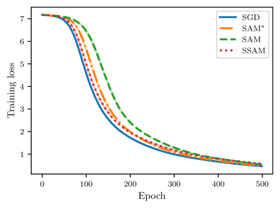
Despite the potential benefit of improved generalization, however, this unusual operation also brings about one critical issue during training. Compared to SGD, as pointed out by Compagnoni et al. (2023) and Kim et al. (2023), SAM dynamics are easier to become trapped in the saddle points and require much more time to escape from them. To see this, let us take the linear autoencoder described in Kunin et al. (2019) as an example. It is known that there is a saddle point of the loss function near the origin and here we compare the escaping efficiency of different optimizers. As shown in Figure 1, we can observe that both SAM and $\mathrm{SAM}^{\ast}$ indeed require more time than SGD to escape from this point and become slower and slower as we gradually increase $\rho$ up to not being able to escape anymore.

To stabilize training neural networks with SAM and its variants, here we propose a simple yet effective strategy by rescaling the gradient norm at point $\boldsymbol{w}_{t}^{asc}$ to the same magnitude as the gradient norm at point $\boldsymbol{w}_{t}$ . In brief, our contributions can be summarized as follows:

1.

We proposed a strategy, dubbed Stable SAM (SSAM), to stabilize training deep neural networks with SAM optimizer. Our strategy is easy to implement and flexible enough to be integrated with any other SAM variants, almost at no computational cost. Most importantly, our strategy does not introduce any additional hyperparameter, tuning which is quite time-consuming in the context of sharpness-based optimization.
2.

We theoretically analyzed the benefits of SAM over SGD in terms of algorithmic stability (Hardt et al., 2016) and found that the superiority of SAM is only assured in a limited regime of learning rate. We further extended the study to SSAM and showed that it allows for a larger learning rate and can consistently perform better than SAM under a mild condition.
3.

We empirically validated the capability of SSAM to stabilize sharpness-aware training and demonstrated its improved generalization performance in real-world problems.

The remainder of the study is organized as follows. Section 2 reviews the related literature, while Section 3 elaborates on the details of the renormalization strategy. Section 4 then provides a theoretical analysis of SAM and SSAM from the perspective of expected excess risk. Finally, before concluding the study, Section 5 presents the experimental results.

2 Related Works

Building upon the seminal work of SAM (Foret et al., 2021), numerous algorithms have been proposed, most of which can be classified into two categories.

The first category continues to improve the generalization performance of SAM. By stretching/shrinking the neighborhood ball according to the magnitude of parameters, ASAM (Kwon et al., 2021) strengthens the connection between sharpness and generalization, which might break up due to model reparameterization. Similarly, instead of defining the neighborhood ball in the Euclidean space, FisherSAM (Kim et al., 2022) runs the SAM update on the statistical manifold induced by the Fisher information matrix. Since one-step gradient ascent may not suffice to accurately approximate the solution of the inner maximization, RSAM (Liu et al., 2022b) was put forward by smoothing the loss landscape with Gaussian filters. This approach is similar to Haruki et al. (2019); Bisla et al. (2022), both of which aim to flatten the loss landscape by convoluting the loss function with stochastic noise. To separate the goal of minimizing the training loss and sharpness, GSAM (Zhuang et al., 2022) was developed to seek a region with both small loss and low sharpness. Contrary to imposing a common weight perturbation within each mini-batch, $\delta$ -SAM (Zhou et al., 2022) uses an approximate per-example perturbation with a theoretically principled weighting factor.

The second category is devoted to reducing the computational cost because SAM involves two gradient backpropagations at each iteration. An early attempt is LookSAM (Liu et al., 2022a), which runs a SAM update every few iterations. Another strategy is RST (Zhao et al., 2022b), according to which SAM and standard training are randomly switched with a scheduled probability. Inspired by the local quadratic structure of the loss landscape, SALA (Tan et al., 2024) uses SAM only at the terminal phase of training when the distance between two consecutive steps is smaller than a threshold. Similarly, AESAM(Jiang et al., 2023) designs an adaptive policy to apply SAM update only in the sharp regions of the loss landscape. ESAM (Du et al., 2022a) and Sparse SAM (Mi et al., 2022) both attempt to perturb a subset of parameters to estimate the sharpness measure, while KSAM (Ni et al., 2022) applies the SAM update to the examples with the highest loss. Another intriguing approach is SAF (Du et al., 2022b), which accelerates the training process by replacing the sharpness measure with a trajectory loss. However, this approach is heavily memory-consuming as it requires saving the output history of each example.

In contrast to these studies, our approach concentrates on improving the training stability of sharpness-aware optimization, functioning as a plug-and-play component for SAM and its variants. Despite its simplicity, our approach is shown to be more robust with large learning rates and can achieve similar or even superior generalization performance compared to the vanilla SAM.

3 Methodology

While there exist some disputes (Dinh et al., 2017; Wen et al., 2024), it is widely appreciated that flat minima empirically generalize better than sharp ones (Keskar et al., 2017; Chaudhari et al., 2019; Kaddour et al., 2022). Motivated by this, SAM actively biases the training towards the flat regions of the loss landscape and seeks a neighborhood with low training losses. In practice, after a series of Taylor approximations, each SAM iterate can be decomposed into two steps,

\displaystyle\boldsymbol{w}_{t}^{asc}=\boldsymbol{w}_{t}+\rho{\nabla F_{\Omega_{t}}(\boldsymbol{w}_{t})},\quad\boldsymbol{w}_{t+1}=\boldsymbol{w}_{t}-\eta\nabla F_{\Omega_{t}}(\boldsymbol{w}_{t}^{asc}),

where $\Omega_{t}$ is a mini-batch of $S$ at $t$ -th step, $\rho>0$ is the perturbation radius, and $\eta$ is the learning rate. By first ascending the weight along $\nabla F_{\Omega_{t}}(\boldsymbol{w}_{t})$ and then descending it along $\nabla F_{\Omega_{t}}(\boldsymbol{w}_{t}^{asc})$ , SAM penalizes the gradient norm (Zhao et al., 2022a; Compagnoni et al., 2023) and consistently minimizes the worse-case loss within the neighborhood, making the found solution more robust to distribution shift and consequently yielding a better generalization.

In contrast to SGD, however, SAM faces a higher risk of getting trapped in the saddle points (Compagnoni et al., 2023; Kim et al., 2023), which may result in suboptimal outcomes (Du et al., 2017; Kleinberg et al., 2018). To gain some quantitative insights into how SAM exacerbates training stability, let us consider the following function (Lucchi et al., 2021),

f(x_{1},x_{2})=\frac{1}{4}x_{1}^{4}-x_{1}x_{2}+\frac{1}{2}x_{2}^{2},

which has a strict saddle point at $(0,0)$ and two global minima at $(-1,-1)$ and $(1,1)$ . Given a random starting point, we want to know whether the training process can converge to one of the global minima.

Algorithm 1 SSAM Optimizer

0: Training set

S=\{(x_{i},y_{i})\}_{i=1}^{n}

, objective function

F_{S}(\boldsymbol{w})

, initial weight

\boldsymbol{w}_{0}\in\mathbb{R}^{d}

, learning rate

\eta>0

, perturbation radius

\rho>0

, training iterations

T

, and base optimizer

\mathcal{A}

(e.g. SGD)

\boldsymbol{w}_{T}

1: for

t=0,1,\cdots,T-1

2: Sample a mini-batch

\Omega_{t}=\{(x_{t_{1}},y_{t_{1}}),\cdots,(x_{t_{b}},y_{t_{b}})\}

;

3: Compute gradient

\boldsymbol{g}_{t}=\nabla_{\boldsymbol{w}}F_{\Omega_{t}}(\boldsymbol{w})|_{\boldsymbol{w}=\boldsymbol{w}_{t}}

of the loss over

\Omega_{t}

;

4: Compute perturbed weight

\boldsymbol{w}^{asc}_{t}=\boldsymbol{w}_{t}+\rho\boldsymbol{g}_{t}

;

5: Compute gradient

\boldsymbol{g}^{asc}_{t}=\nabla_{\boldsymbol{w}}F_{\Omega_{t}}(\boldsymbol{w})|_{\boldsymbol{w}=\boldsymbol{w}^{asc}_{t}}

of the loss over the same

\Omega_{t}

;

6: Renormalize gradient as

\boldsymbol{g}^{asc}_{t}=\frac{\|\boldsymbol{g}_{t}\|_{2}}{\|\boldsymbol{g}^{asc}_{t}\|_{2}}\boldsymbol{g}^{asc}_{t}

;

7: Update weight with base optimizer

\mathcal{A}

, e.g.

\boldsymbol{w}_{t+1}=\boldsymbol{w}_{t}-\eta\boldsymbol{g}^{asc}_{t}

;

8: end for

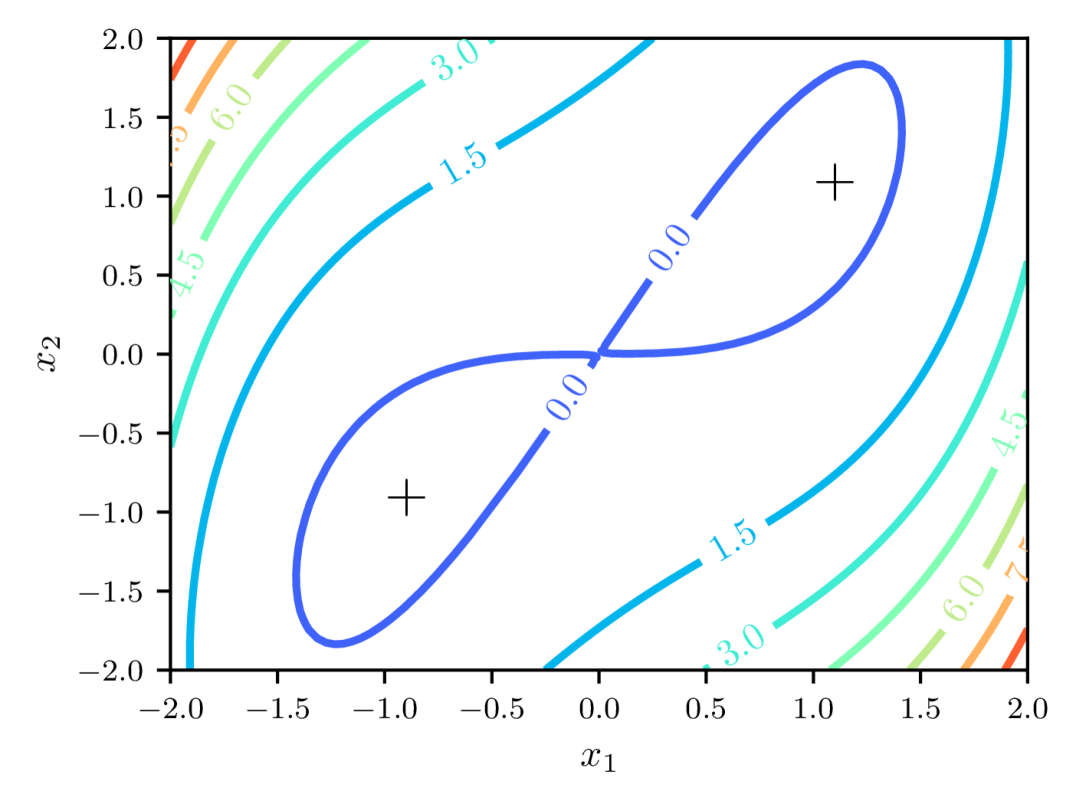
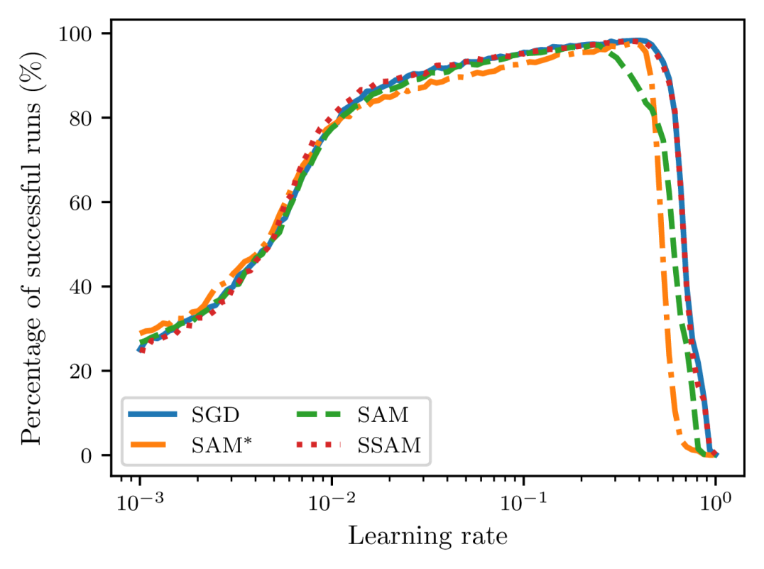
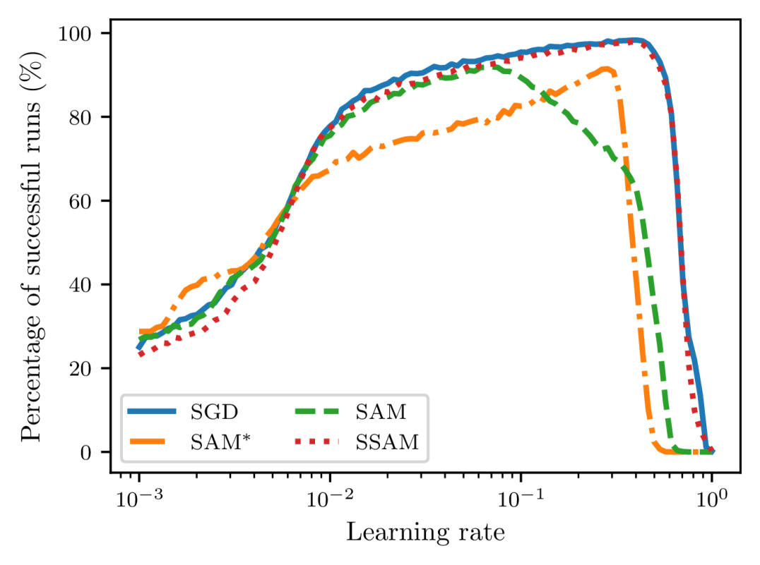
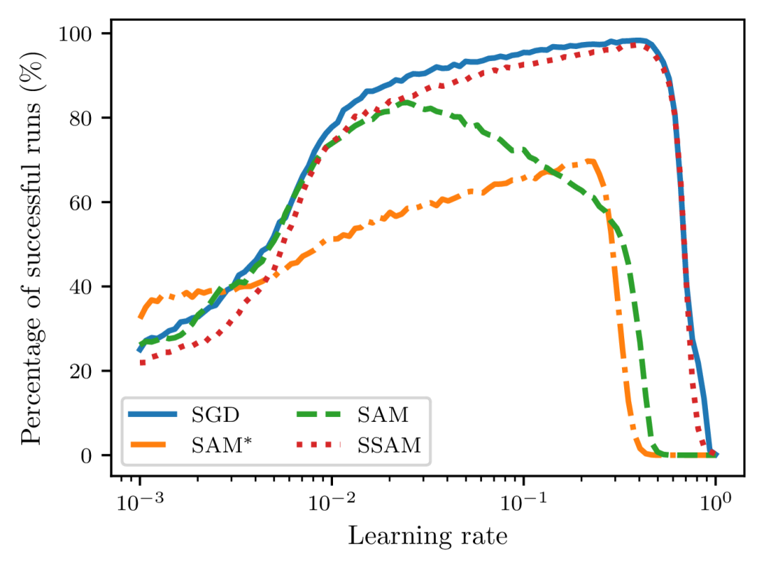
For this purpose, we select 100 different learning rates that are equispaced between 0.001 and 0.3 on the logarithm scale. For each learning rate, we then uniformly sample 10000 random points from the square $[-2,2]\times[-2,2]$ and report the total percentage of runs that eventually converge to the global minima. We mark the runs that get stuck in the saddle point or fail to converge as unsuccessful runs. To introduce stochasticity during training, we manually perturb the gradient with zero-mean Gaussian noise with a variance of $0.005$ . As shown in Figure 2, the failed percentage of SAM and $\mathrm{SAM}^{\ast}$ first blow up when we gradually increase the learning rate, suggesting that a smaller learning rate is necessary for sharpness-aware training to ensure convergence. Moreover, we can observe that SGD always achieves the highest rate of successful training, while $\mathrm{SAM}^{\ast}$ is the most unstable optimizer. Notice that the stability of sharpness-aware training also heavily relies on the perturbation radius $\rho$ . Often, a larger $\rho$ corresponds to a lower percentage of successful runs. This indicates that both SAM and $\mathrm{SAM}^{\ast}$ become more and more difficult to escape from the saddle point $(0,0)$ .

To address this issue, we propose a simple strategy, dubbed SSAM, to improve the stability of sharpness-aware training. As shown in Algorithm 1²²2A PyTorch implementation is available at https://github.com/cltan023/stablesam2024., the only difference from SAM is that we include an extra renormalization step (line 6) to ensure that the gradient norm of the descent step does not exceed that of the ascent step. The ratio, $\gamma_{t}=\|\nabla F_{\Omega_{t}}(\boldsymbol{w}_{t})\|_{2}/\|\nabla F_{\Omega_{t}}(\boldsymbol{w}_{t}^{asc})\|_{2}$ , which we refer to as the renormalization factor, can be interpreted as follows. When $\|\nabla F_{\Omega_{t}}(\boldsymbol{w}_{t}^{asc})\|_{2}$ is larger than $\|\nabla F_{\Omega_{t}}(\boldsymbol{w}_{t})\|_{2}$ , we downscale the norm of $\nabla F_{\Omega_{t}}(\boldsymbol{w}_{t}^{asc})$ to ensure that the iterates move in a smaller step towards the flat regions and thus we can reduce the chance of fluctuation and divergence. In contrast, when $\|\nabla F_{\Omega_{t}}(\boldsymbol{w}_{t}^{asc})\|_{2}$ is smaller than $\|\nabla F_{\Omega_{t}}(\boldsymbol{w}_{t})\|_{2}$ , a situation that may occur near the saddle points, we upscale the norm of $\nabla F_{\Omega_{t}}(\boldsymbol{w}_{t}^{asc})$ to incur a larger perturbation to improve the escaping efficiency.

After applying the renormalization strategy, as shown in Figure 2, we can observe that this issue can be remedied to a large extent because the curve of SSAM now remains approximately the same as SGD even for large learning rates. Similar results for realistic neural networks can also be found in Appendix A. It should be clarified that the analysis here is not from the generalization perspective, but instead from the optimization perspective only. Compared to SAM, our approach does not introduce any additional hyperparameter so that it can be integrated with other SAM variants almost at no computational cost.

4 Theoretical Analysis

The generalization ability of sharpness-aware training was initially studied by the PAC-Bayesian theory (Foret et al., 2021; Yue et al., 2023; Zhuang et al., 2022). This approach, however, is fundamentally limited since the generalization bound is focused on the worst-case perturbation rather than the realistic one-step ascent approximation (Wen et al., 2022). For a certain class of problems, an analysis from the perspective of implicit bias suggests that SAM can always choose a better solution than SGD (Andriushchenko and Flammarion, 2022). In the small learning rate regime, Compagnoni et al. (2023) further characterized the continuous-time models for SAM in the form of a stochastic differential equation and concluded that SAM is attracted to saddle points under some realistic conditions, an observation which has also been unveiled by Kim et al. (2023). Moreover, Bartlett et al. (2023) argued that SAM converges to a cycle that oscillates between the minimum along the principal direction of the Hessian of the loss function. Different from these studies, here we investigate the generalization performance of SAM via algorithmic stability (Bousquet and Elisseeff, 2002; Hardt et al., 2016) and together with its convergence properties present an upper bound over its expected excess risk. We first show that SAM consistently generalizes better than SGD, though a much smaller learning rate is required. Finally, we show how our proposed method, SSAM, extends the regime of learning rate and can achieve a better generalization performance than SAM.

4.1 Notations and Preliminaries

Let $X\subset\mathbb{R}^{p}$ and $Y\subset\mathbb{R}$ denote the feature and label space, respectively. We consider a training set $S$ of $n$ examples, each of which is randomly sampled from an unknown distribution $\mathfrak{D}$ over the data space $Z=X\times Y$ . Given a learning algorithm $\mathcal{A}$ , it learns a hypothesis that relates the input $x\in X$ to the output $y\in Y$ . For deep neural networks, the learned hypothesis is parameterized by the network parameters $\boldsymbol{w}\in\mathbb{R}^{d}$ .

Suppose $f(\boldsymbol{w},z):\mathbb{R}^{d}\times Z\mapsto\mathbb{R}_{+}$ is a non-negative cost function, we then can define the population risk

F_{\mathfrak{D}}(\boldsymbol{w})=\mathbb{E}_{z\sim\mathfrak{D}}\left[f(\boldsymbol{w},z)\right],

and the empirical risk

F_{S}(\boldsymbol{w})=\frac{1}{n}\sum_{i=1}^{n}f(\boldsymbol{w},z_{i}).

In practice, we cannot compute $F_{\mathfrak{D}}(\boldsymbol{w})$ directly since the data distribution $\mathfrak{D}$ is unknown. However, once the training set $S$ is given, we have access to its estimation and can minimize the empirical risk $F_{S}(\boldsymbol{w})$ instead, a process which is often referred to as empirical risk minimization. Let $\boldsymbol{w}_{\mathcal{A},S}$ be the output returned by minimizing the empirical risk $F_{S}(\boldsymbol{w})$ with learning algorithm $\mathcal{A}$ , and $\boldsymbol{w}_{\mathfrak{D}}^{*}$ be one minimizer of the population risk $F_{\mathfrak{D}}(\boldsymbol{w})$ , namely, $\boldsymbol{w}_{\mathfrak{D}}^{*}\in\arg\min_{\boldsymbol{w}}F_{\mathfrak{D}}(\boldsymbol{w})$ . Since $\boldsymbol{w}_{\mathcal{A},S}$ in high probability will not be the same with $\boldsymbol{w}_{\mathfrak{D}}^{*}$ , we are interested in how far $\boldsymbol{w}_{\mathcal{A},S}$ deviates from $\boldsymbol{w}_{\mathfrak{D}}^{*}$ when evaluated on an unseen example $z\sim\mathfrak{D}$ .

A natural measure to quantify this difference is the so-called expected excess risk,

	$\displaystyle\varepsilon_{exc}$	$\displaystyle=\mathbb{E}\left[F_{\mathfrak{D}}(\boldsymbol{w}_{\mathcal{A},S})-F_{\mathfrak{D}}(\boldsymbol{w}_{\mathfrak{D}}^{*})\right]$
		$\displaystyle=\underbrace{\mathbb{E}\left[F_{\mathfrak{D}}(\boldsymbol{w}_{\mathcal{A},S})-F_{S}(\boldsymbol{w}_{\mathcal{A},S})\right]}_{\varepsilon_{gen}}+\underbrace{\mathbb{E}\left[F_{S}(\boldsymbol{w}_{\mathcal{A},S})-F_{S}(\boldsymbol{w}_{S}^{})\right]}_{\varepsilon_{opt}}+\underbrace{\mathbb{E}\left[F_{S}(\boldsymbol{w}_{S}^{})-F_{\mathfrak{D}}(\boldsymbol{w}_{\mathfrak{D}}^{*})\right]}_{\varepsilon_{approx}},$

where $\boldsymbol{w}_{S}^{*}\in\arg\min_{\boldsymbol{w}}F_{S}(\boldsymbol{w})$ . Since $\boldsymbol{w}_{\mathfrak{D}}^{*}$ remains constant for the population risk $F_{\mathfrak{D}}(\boldsymbol{w})$ which depends only on the data distribution and loss function, it follows that the expected approximation error $\varepsilon_{approx}=\mathbb{E}\left[F_{S}(\boldsymbol{w}_{S}^{*})-F_{\mathfrak{D}}(\boldsymbol{w}_{\mathfrak{D}}^{*})\right]=\mathbb{E}\left[F_{S}(\boldsymbol{w}_{S}^{*})-F_{S}(\boldsymbol{w}_{\mathfrak{D}}^{*})\right]\leq 0$ . Therefore, it often suffices to obtain tight control of the expected excess risk $\varepsilon_{exc}$ by bounding the expected generalization error³³3It is worth noting that the difference between the test error and the training error in some literature is referred to as generalization gap and the test error alone goes by generalization error. $\varepsilon_{gen}$ and the expected optimization error $\varepsilon_{opt}$ .

For learning algorithms based on iterative optimization, $\varepsilon_{opt}$ in many cases can be analyzed via a convergence analysis (Bubeck et al., 2015). Meanwhile, to derive an upper bound over $\varepsilon_{gen}$ , we can use the following theorem, which is due to Hardt et al. (2016), indicating that the generalization error could be bounded via the uniform stability (Bousquet and Elisseeff, 2002). Indeed, the uniform stability characterizes how sensitive the output of the learning algorithm $\mathcal{A}$ is when a single example in the training set $S$ is modified.

Theorem 1 (Generalization error under $\varepsilon$ -uniformly stability)

Let $S$ and $S^{\prime}$ denote two training sets i.i.d. sampled from the same data distribution $\mathfrak{D}$ such that $S$ and $S^{\prime}$ differ in at most one example. A learning algorithm $\mathcal{A}$ is $\varepsilon$ -uniformly stable if and only if for all samples $S$ and $S^{\prime}$ , the following inequality holds

\sup_{z}\mathbb{E}|f(\boldsymbol{w}_{\mathcal{A},S},z)-f(\boldsymbol{w}_{\mathcal{A},S^{\prime}},z)|\leq\varepsilon.

Furthermore, if $\mathcal{A}$ is $\varepsilon$ -uniformly stable, the expected generalization error $\varepsilon_{gen}$ is upper bounded by $\varepsilon$ , namely,

\mathbb{E}\left[F_{\mathfrak{D}}(\boldsymbol{w}_{\mathcal{A},S})-F_{S}(\boldsymbol{w}_{\mathcal{A},S})\right]\leq\varepsilon.

To ease notation, we use $f(\boldsymbol{w})$ interchangeably with $f(\boldsymbol{w},z)$ in the sequel as long as it is clear from the context that $z$ is being held constant or can be understood from prior information.

4.2 Expected Excess Risk Analysis of SAM

In this section, we first investigate the stability of SAM and then its convergence property, together yielding an upper bound over the expected excess risk $\varepsilon_{exc}$ . We restrict our attention to the strongly convex case so that we can compare against known results, particularly from Hardt et al. (2016).

4.2.1 Stability

Consider the optimization trajectories $\boldsymbol{w}_{0},\boldsymbol{w}_{1},\cdots,\boldsymbol{w}_{T}$ and $\boldsymbol{v}_{0},\boldsymbol{v}_{1},\cdots,\boldsymbol{v}_{T}$ induced by running SAM for $T$ steps on sample $S$ and $S^{\prime}$ , which differ from each other only by one example. Suppose that the loss function $f(\boldsymbol{w},z)$ is $G$ -Lipschitz with respect to the first argument, then it holds for all $z\in Z$ that

|f(\boldsymbol{v}_{T},z)-f(\boldsymbol{w}_{T},z)|\leq G\|\boldsymbol{v}_{T}-\boldsymbol{w}_{T}\|_{2}.

(1)

Therefore, the remaining step in our setup is to upper bound $\|\boldsymbol{v}_{T}-\boldsymbol{w}_{T}\|_{2}$ , which can be recursively controlled by the growth rate. Since $S$ and $S^{\prime}$ differ in only one example, at every step $t$ , the selected examples from $S$ and $S^{\prime}$ , say $z$ and $z^{\prime}$ , are either the same or not. In the lemma below, we show that $\|\boldsymbol{v}_{t}-\boldsymbol{w}_{t}\|_{2}$ is contracting when $z$ and $z^{\prime}$ are the same.

Lemma 2

Assume that the per-example loss function $f(\boldsymbol{w},z)$ is $\mu$ -strongly convex, $L$ -smooth, and $G$ -Lipschitz continuous with respect to the first argument $\boldsymbol{w}$ . Suppose that at step $t$ , the examples selected by SAM are the same in $S$ and $S^{\prime}$ and the update rules are denoted by $\boldsymbol{w}_{t+1}=\boldsymbol{w}_{t}-\eta\nabla f(\boldsymbol{w}_{t}^{asc},z)$ and $\boldsymbol{v}_{t+1}=\boldsymbol{v}_{t}-\eta\nabla f(\boldsymbol{v}_{t}^{asc},z)$ , respectively. Then, it follows that

\|\boldsymbol{v}_{t+1}-\boldsymbol{w}_{t+1}\|_{2}\leq\left(1-\left(1+\mu\rho\right)\frac{\eta\mu L}{\mu+L}\right)\|\boldsymbol{v}_{t}-\boldsymbol{w}_{t}\|_{2},

(2)

where the learning rate $\eta$ satisfies that

\eta\leq\frac{2}{\mu+L}-\frac{\mu+L}{2\mu L(\mu/\rho L^{2}+1)}.

(3)

Proof To prove this result, we first would like to lower bound the term $\|\boldsymbol{v}_{t}^{asc}-\boldsymbol{w}_{t}^{asc}\|_{2}^{2}$ as follows:

	$\displaystyle\\|\boldsymbol{v}_{t}^{asc}-\boldsymbol{w}_{t}^{asc}\\|_{2}^{2}$	$\displaystyle=\\|\boldsymbol{v}_{t}-\boldsymbol{w}_{t}\\|_{2}^{2}+2\rho\left<\boldsymbol{v}_{t}-\boldsymbol{w}_{t},\nabla f(\boldsymbol{v}_{t})-\nabla f(\boldsymbol{w}_{t})\right>+\rho^{2}\\|\nabla f(\boldsymbol{v}_{t})-\nabla f(\boldsymbol{w}_{t})\\|_{2}^{2}$
		$\displaystyle\geq(1+2\mu\rho)\\|\boldsymbol{v}_{t}-\boldsymbol{w}_{t}\\|_{2}^{2}+\rho^{2}\\|\nabla f(\boldsymbol{v}_{t})-\nabla f(\boldsymbol{w}_{t})\\|_{2}^{2}$
		$\displaystyle\geq(1+\mu\rho)\\|\boldsymbol{v}_{t}-\boldsymbol{w}_{t}\\|_{2}^{2}+({\mu\rho}/{L^{2}}+\rho^{2})\\|\nabla f(\boldsymbol{v}_{t})-\nabla f(\boldsymbol{w}_{t})\\|_{2}^{2}.$

According to the update rule, we further have

	$\displaystyle\\|\boldsymbol{v}_{t+1}-\boldsymbol{w}_{t+1}\\|_{2}^{2}={}\\|\boldsymbol{v}_{t}-\eta\nabla f(\boldsymbol{v}_{t}^{asc})-\left(\boldsymbol{w}_{t}-\eta\nabla f(\boldsymbol{w}_{t}^{asc})\right)\\|_{2}^{2}$
	$\displaystyle{}={}\\|\boldsymbol{v}_{t}-\boldsymbol{w}_{t}\\|_{2}^{2}-2\eta\left<\boldsymbol{v}_{t}-\boldsymbol{w}_{t},\nabla f(\boldsymbol{v}_{t}^{asc})-\nabla f(\boldsymbol{w}_{t}^{asc})\right>+\eta^{2}\\|\nabla f(\boldsymbol{v}_{t}^{asc})-\nabla f(\boldsymbol{w}_{t}^{asc})\\|_{2}^{2}$
	$\displaystyle=\begin{aligned} &\\|\boldsymbol{v}_{t}-\boldsymbol{w}_{t}\\|_{2}^{2}-2\eta\left<\boldsymbol{v}_{t}^{asc}-\boldsymbol{w}_{t}^{asc},\nabla f(\boldsymbol{v}_{t}^{asc})-\nabla f(\boldsymbol{w}_{t}^{asc})\right>\\ &\quad+2\rho\eta\left<\nabla f(\boldsymbol{v}_{t})-\nabla f(\boldsymbol{w}_{t}),\nabla f(\boldsymbol{v}_{t}^{asc})-\nabla f(\boldsymbol{w}_{t}^{asc})\right>+\eta^{2}\\|\nabla f(\boldsymbol{v}_{t}^{asc})-\nabla f(\boldsymbol{w}_{t}^{asc})\\|_{2}^{2}\end{aligned}$
	$\displaystyle\stackrel{{\scriptstyle①}}{{\leq}}\begin{aligned} &\left(1-2\left(1+\mu\rho\right)\frac{\eta\mu L}{\mu+L}\right)\\|\boldsymbol{v}_{t}-\boldsymbol{w}_{t}\\|_{2}^{2}-2\left(\frac{\mu\rho}{L^{2}}+\rho^{2}\right)\frac{\eta\mu L}{\mu+L}\\|\nabla f(\boldsymbol{v}_{t})-\nabla f(\boldsymbol{w}_{t})\\|_{2}^{2}\\ &\quad+2\rho\eta\left<\nabla f(\boldsymbol{v}_{t})-\nabla f(\boldsymbol{w}_{t}),\nabla f(\boldsymbol{v}_{t}^{asc})-\nabla f(\boldsymbol{w}_{t}^{asc})\right>+\left(\eta^{2}-\frac{2\eta}{\mu+L}\right)\\|\nabla f(\boldsymbol{v}_{t}^{asc})-\nabla f(\boldsymbol{w}_{t}^{asc})\\|_{2}^{2}\end{aligned}$
	$\displaystyle\stackrel{{\scriptstyle②}}{{\leq}}\begin{aligned} &\left(1-2\left(1+\mu\rho\right)\frac{\eta\mu L}{\mu+L}\right)\\|\boldsymbol{v}_{t}-\boldsymbol{w}_{t}\\|_{2}^{2}+\left[\frac{\rho^{2}\eta}{\frac{2}{\mu+L}-\eta}-2\left(\frac{\mu\rho}{L^{2}}+\rho^{2}\right)\frac{\eta\mu L}{\mu+L}\right]\\|\nabla f(\boldsymbol{v}_{t})-\nabla f(\boldsymbol{w}_{t})\\|_{2}^{2}\\ &\quad+\left(\eta^{2}-\frac{2\eta}{\mu+L}\right)\left[\left(\nabla f\left(\boldsymbol{v}_{t}^{asc}\right)-\nabla f\left(\boldsymbol{w}_{t}^{asc}\right)\right)-\frac{\rho}{\frac{2}{\mu+L}-\eta}\left(\nabla f\left(\boldsymbol{v}_{t}\right)-\nabla f\left(\boldsymbol{w}_{t}\right)\right)\right]^{2}\end{aligned}$
	$\displaystyle\stackrel{{\scriptstyle③}}{{\leq}}{}\left(1-2\left(1+\mu\rho\right)\frac{\eta\mu L}{\mu+L}\right)\\|\boldsymbol{v}_{t}-\boldsymbol{w}_{t}\\|_{2}^{2},$

where $①$ is due to the coercivity of the loss function (cf. Appendix B) that

\left<\nabla f(\boldsymbol{v}_{t}^{asc})-\nabla f(\boldsymbol{w}_{t}^{asc}),\boldsymbol{v}_{t}^{asc}-\boldsymbol{w}_{t}^{asc}\right>\geq\frac{\mu L}{\mu+L}\|\boldsymbol{v}_{t}^{asc}-\boldsymbol{w}_{t}^{asc}\|_{2}^{2}+\frac{1}{\mu+L}\|\nabla f(\boldsymbol{v}_{t}^{asc})-\nabla f(\boldsymbol{w}_{t}^{asc})\|_{2}^{2}.

Moreover, ③ holds since the last two terms of ② are smaller than zero provided that the learning rate $\eta$ satisfies the given condition. Consequently, we have

\|\boldsymbol{v}_{t+1}-\boldsymbol{w}_{t+1}\|_{2}\leq\left(1-2\left(1+\mu\rho\right)\frac{\eta\mu L}{\mu+L}\right)^{1/2}\|\boldsymbol{v}_{t}-\boldsymbol{w}_{t}\|_{2}\leq\left(1-\left(1+\mu\rho\right)\frac{\eta\mu L}{\mu+L}\right)\|\boldsymbol{v}_{t}-\boldsymbol{w}_{t}\|_{2},

where the last inequality is due to the fact that $\sqrt{1-x}\leq 1-x/2$ holds for all $x\in[0,1]$ .

Remark 3

To ensure that the learning rate $\eta$ is feasible, the right-hand side of (3) should be at least larger than zero. This holds for any perturbation radius $\rho>0$ if $\mu=L$ . However, if $\mu<L$ , we further need to require that $\rho<4\mu^{2}/L(L-\mu)^{2}$ . It is also worth noting that the following inequality holds for all $\rho>0$

\frac{2}{\mu+L}-\frac{\mu+L}{2\mu L(\mu/\rho L^{2}+1)}<\frac{2}{(1+\mu\rho)(\mu+L)},

implying that the contractivity of (2) can be guaranteed.

On the other hand, with probability $1/n$ , the examples selected by SAM, say $z$ and $z^{\prime}$ , are different in both $S$ and $S^{\prime}$ . In this case, we can simply bound the growth in $\|\boldsymbol{v}_{t}-\boldsymbol{w}_{t}\|_{2}$ by the norms of $\nabla f(\boldsymbol{w},z)$ and $\nabla f(\boldsymbol{v},z^{\prime})$ .

Lemma 4

Assume the same settings as in Lemma 2. For the $t$ -th iteration, suppose that the examples selected by SAM are different in $S$ and $S^{\prime}$ and the update rules are denoted by $\boldsymbol{w}_{t+1}=\boldsymbol{w}_{t}-\eta\nabla f(\boldsymbol{w}_{t}^{asc},z)$ and $\boldsymbol{v}_{t+1}=\boldsymbol{v}_{t}-\eta\nabla f(\boldsymbol{v}_{t}^{asc},z^{\prime})$ , respectively. Consequently, we have

\|\boldsymbol{v}_{t+1}-\boldsymbol{w}_{t+1}\|_{2}\leq\left(1-\left(1+\mu\rho\right)\frac{\eta\mu L}{\mu+L}\right)\|\boldsymbol{v}_{t}-\boldsymbol{w}_{t}\|_{2}+2\eta G.

Proof The proof is straightforward. It follows immediately

	$\displaystyle\\|\boldsymbol{v}_{t+1}-\boldsymbol{w}_{t+1}\\|_{2}$	$\displaystyle=\\|\boldsymbol{v}_{t}-\eta\nabla f(\boldsymbol{v}_{t}^{asc},z^{\prime})-\left(\boldsymbol{w}_{t}-\eta\nabla f(\boldsymbol{w}_{t}^{asc},z^{\prime})\right)-\eta\left(\nabla f(\boldsymbol{w}_{t}^{asc},z^{\prime})-\nabla f(\boldsymbol{w}_{t}^{asc},z)\right)\\|_{2}$
		$\displaystyle\leq\\|\boldsymbol{v}_{t}-\eta\nabla f(\boldsymbol{v}_{t}^{asc},z^{\prime})-\left(\boldsymbol{w}_{t}-\eta\nabla f(\boldsymbol{w}_{t}^{asc},z^{\prime})\right)\\|_{2}+\eta\\|\nabla f(\boldsymbol{w}_{t}^{asc},z^{\prime})-\nabla f(\boldsymbol{w}_{t}^{asc},z)\\|_{2}$
		$\displaystyle\leq\left(1-\left(1+\mu\rho\right)\frac{\eta\mu L}{\mu+L}\right)\\|\boldsymbol{v}_{t}-\boldsymbol{w}_{t}\\|_{2}+2\eta G,$

where the last inequality comes from Lemma 2.
With the above two lemmas, we are now ready to give an upper bound over the expected generalization error of SAM.

Theorem 5

Assume that the per-example loss function $f(\boldsymbol{w},z)$ is $\mu$ -strongly convex, $L$ -smooth, and $G$ -Lipschitz continuous with respect to the first argument $\boldsymbol{w}$ . Suppose we run the SAM iteration with a constant learning rate $\eta$ satisfying (3) for $T$ steps. Then, SAM satisfies uniform stability with

\varepsilon_{\mathrm{gen}}^{\mathrm{sam}}\leq\frac{2G^{2}(\mu+L)}{n\mu L(1+\mu\rho)}\left\{1-\left[1-\left(1+\mu\rho\right)\frac{\eta\mu L}{\mu+L}\right]^{T}\right\}.

Proof Define $\delta_{t}=\|\boldsymbol{w}_{t}-\boldsymbol{v}_{t}\|_{2}$ to denote the Euclidean distance between $\boldsymbol{w}_{t}$ and $\boldsymbol{v}_{t}$ as training progresses. Observe that at any step $t\leq T$ , with a probability $1-1/n$ , the selected examples from $S$ and $S^{\prime}$ are the same. In contrast, with a probability of $1/n$ , the selected examples are different. This is because $S$ and $S^{\prime}$ only differ by one example. Therefore, from Lemmas 2 and 4, we conclude that

	$\displaystyle\mathbb{E}[\delta_{t}]$	$\displaystyle\leq\left(1-\frac{1}{n}\right)\left(1-\left(1+\mu\rho\right)\frac{\eta\mu L}{\mu+L}\right)\mathbb{E}[\delta_{t-1}]+\frac{1}{n}\left(1-\left(1+\mu\rho\right)\frac{\eta\mu L}{\mu+L}\right)\mathbb{E}[\delta_{t-1}]+\frac{2\eta G}{n}$
		$\displaystyle=\left(1-\left(1+\mu\rho\right)\frac{\eta\mu L}{\mu+L}\right)\mathbb{E}[\delta_{t-1}]+\frac{2\eta G}{n}.$

Unraveling the above recursion yields

\displaystyle\mathbb{E}[\delta_{T}]\leq\frac{2\eta G}{n}\sum_{t=0}^{T-1}\left(1-\left(1+\mu\rho\right)\frac{\eta\mu L}{\mu+L}\right)^{t}=\frac{2G(\mu+L)}{n\mu L(1+\mu\rho)}\left\{1-\left[1-\left(1+\mu\rho\right)\frac{\eta\mu L}{\mu+L}\right]^{T}\right\}.

Plugging this inequality into (1), we complete the proof.
In the same strongly convex setting, it is known that SGD allows for a larger learning rate (namely, $\eta\leq\frac{2}{\mu+L}$ ) to attain a similar generalization bound (Hardt et al., 2016, Lemma 3.7). However, when both SGD and SAM use a constant learning rate satisfying (3), the following corollary suggests that SAM consistently generalizes better than SGD.

Corollary 6

Assume the same settings as in Theorem 5. Suppose we run SGD and SAM with a constant learning rate $\eta$ satisfying (3) for $T$ steps. Then, SAM consistently achieves a tighter generalization bound than SGD.

Proof Following Hardt et al. (2016, Theorem 3.9), we can derive a similar generalization bound for SGD as follows

\varepsilon_{\mathrm{gen}}^{\mathrm{sgd}}\leq\frac{2G^{2}(\mu+L)}{n\mu L}\left\{1-\left[1-\frac{\eta\mu L}{\mu+L}\right]^{T}\right\}.

Define $q(x)=a(1-x)^{T}-(1-ax)^{T}$ , where $a=1+\mu\rho$ and $x=\frac{\eta\mu L}{\mu+L}$ . Note that $a>1$ and $0<ax<1$ . With a simple calculation, we have

q^{\prime}(x)=aT\left[\left(1-ax\right)^{T-1}-\left(1-x\right)^{T-1}\right],

implying that $q^{\prime}(x)\leq 0$ for any $T\geq 1$ and as a result we have $q(x)\leq a-1$ . Then, it follows that

\varepsilon_{\mathrm{gen}}^{\mathrm{sam}}=\frac{2G^{2}(\mu+L)}{n\mu L(1+\mu\rho)}\left\{1-\left[1-\left(1+\mu\rho\right)\frac{\eta\mu L}{\mu+L}\right]^{T}\right\}\leq\frac{2G^{2}(\mu+L)}{n\mu L}\left\{1-\left[1-\frac{\eta\mu L}{\mu+L}\right]^{T}\right\}=\varepsilon_{\mathrm{gen}}^{\mathrm{sgd}},

thus concluding the proof.

4.2.2 Convergence

From the perspective of convergence, we can further prove that SAM converges to a noisy ball if the learning rate $\eta$ is fixed. Let $z_{t}$ be the example that is chosen by SAM at $t$ -th step and $\nabla f(\boldsymbol{w}_{t}^{asc})=\nabla f\left(\boldsymbol{w}_{t}+\rho\nabla f\left(\boldsymbol{w}_{t},z_{t}\right),z_{t}\right)$ be the stochastic gradient of the descent step. It is worth noting that the same example $z_{t}$ is used in the ascent and descent steps. The following lemma shows that $\nabla f(\boldsymbol{w}_{t}^{asc})$ may not be well-aligned with the full-batch gradient $\nabla F_{S}(\boldsymbol{w}_{t})$ .

Lemma 7

Assume the loss function $f(\boldsymbol{w},z)$ is $\mu$ -strongly convex, $L$ -smooth, and $G$ -Lipschitz continuous with respect to the first argument $\boldsymbol{w}$ . Then, we have for all $\boldsymbol{w}_{t}\in\mathbb{R}^{d}$ ,

\mathbb{E}\left<\nabla f(\boldsymbol{w}_{t}^{asc}),\nabla F_{S}(\boldsymbol{w}_{t})\right>\geq\rho(\mu+L)\left\|\nabla F_{S}(\boldsymbol{w}_{t})\right\|_{2}^{2}-\frac{\rho^{2}L^{2}G^{2}}{2}.

Proof First, it is easy to check that $F_{S}(\boldsymbol{w})$ is $\mu$ -strongly convex, $L$ -smooth, and $G$ -Lipschitz continuous with respect to the first argument $\boldsymbol{w}$ as well. Let $\widehat{\boldsymbol{w}}_{t}^{asc}=\boldsymbol{w}_{t}+\rho\nabla F_{S}(\boldsymbol{w}_{t})$ , we have

	$\displaystyle\left<\nabla f(\boldsymbol{w}_{t}^{asc})-\nabla f(\widehat{\boldsymbol{w}}_{t}^{asc}),\nabla F_{S}(\boldsymbol{w}_{t})\right>$	$\displaystyle\leq\frac{1}{2}\left\\|\nabla f(\boldsymbol{w}_{t}^{asc})-\nabla f(\widehat{\boldsymbol{w}}_{t}^{asc})\right\\|_{2}^{2}+\frac{1}{2}\left\\|\nabla F_{S}(\boldsymbol{w}_{t})\right\\|_{2}^{2}$
		$\displaystyle\leq\frac{\rho^{2}L^{2}}{2}\left\\|\nabla f(\boldsymbol{w}_{t})-\nabla F_{S}(\boldsymbol{w}_{t})\right\\|_{2}^{2}+\frac{1}{2}\left\\|\nabla F_{S}(\boldsymbol{w}_{t})\right\\|_{2}^{2}.$

After taking the expectation, it follows that

\mathbb{E}\left<\nabla f(\boldsymbol{w}_{t}^{asc})-\nabla f(\widehat{\boldsymbol{w}}_{t}^{asc}),\nabla F_{S}(\boldsymbol{w}_{t})\right>\leq\frac{\rho^{2}L^{2}G^{2}}{2}+\frac{1-\rho^{2}L^{2}}{2}\left\|\nabla F_{S}(\boldsymbol{w}_{t})\right\|_{2}^{2}.

On the other hand,

	$\displaystyle\mathbb{E}\left<\nabla f(\widehat{\boldsymbol{w}}_{t}^{asc}),\nabla F_{S}(\boldsymbol{w}_{t})\right>$	$\displaystyle=\left<\nabla F_{S}(\widehat{\boldsymbol{w}}_{t}^{asc}),\nabla F_{S}(\boldsymbol{w}_{t})\right>$
		$\displaystyle=\left<\nabla F_{S}(\widehat{\boldsymbol{w}}_{t}^{asc})-\nabla F_{S}(\boldsymbol{w}_{t}),\nabla F_{S}(\boldsymbol{w}_{t})\right>+\left\\|\nabla F_{S}(\boldsymbol{w}_{t})\right\\|_{2}^{2}$
		$\displaystyle=\frac{1}{\rho}\left<\nabla F_{S}(\boldsymbol{w}+\rho\nabla F_{S}(\boldsymbol{w}_{t}))-\nabla F_{S}(\boldsymbol{w}_{t}),\rho\nabla F_{S}(\boldsymbol{w}_{t})\right>+\left\\|\nabla F_{S}(\boldsymbol{w}_{t})\right\\|_{2}^{2}$
		$\displaystyle\geq\left(1+\mu\rho\right)\left\\|\nabla F_{S}(\boldsymbol{w}_{t})\right\\|_{2}^{2}.$

Combining the above results, we have

	$\displaystyle\mathbb{E}\left<\nabla f(\boldsymbol{w}_{t}^{asc}),\nabla F_{S}(\boldsymbol{w}_{t})\right>$	$\displaystyle=\mathbb{E}\left<\nabla f(\boldsymbol{w}_{t}^{asc})-\nabla f(\widehat{\boldsymbol{w}}_{t}^{asc}),\nabla F_{S}(\boldsymbol{w}_{t})\right>+\mathbb{E}\left<\nabla f(\widehat{\boldsymbol{w}}_{t}^{asc}),\nabla F_{S}(\boldsymbol{w}_{t})\right>$
		$\displaystyle\geq\left(\frac{1+\rho^{2}L^{2}}{2}+\mu\rho\right)\left\\|\nabla F_{S}(\boldsymbol{w}_{t})\right\\|_{2}^{2}-\frac{\rho^{2}L^{2}G^{2}}{2}$
		$\displaystyle\geq\rho(\mu+L)\left\\|\nabla F_{S}(\boldsymbol{w}_{t})\right\\|_{2}^{2}-\frac{\rho^{2}L^{2}G^{2}}{2},$

completing the proof.

Theorem 8

Assume that the per-example loss function $f(\boldsymbol{w},z)$ is $\mu$ -strongly convex, $L$ -smooth and $G$ -Lipschitz continuous with respect to the first argument $\boldsymbol{w}$ . Consider the sequence $\boldsymbol{w}_{0},\boldsymbol{w}_{1},\cdots,\boldsymbol{w}_{T}$ generated by running SAM with a constant learning rate $\eta$ for $T$ steps. Let $\boldsymbol{w}^{*}\in\arg\inf_{\boldsymbol{w}}F_{S}(\boldsymbol{w})$ , it follows that

\displaystyle\varepsilon_{\mathrm{opt}}^{\mathrm{sam}}=\mathbb{E}\left[F_{S}(\boldsymbol{w}_{T})-F_{S}(\boldsymbol{w}^{*})\right]\leq\left[1-2\eta\mu\rho(\mu+L)\right]^{T}\mathbb{E}\left[F_{S}(\boldsymbol{w}_{0})-F_{S}(\boldsymbol{w}^{*})\right]+\frac{LG^{2}\left(\rho^{2}L+\eta\right)}{4\mu\rho\left(\mu+L\right)}.

Proof From Taylor’s theorem, there exists a $\widehat{\boldsymbol{w}}_{t}$ such that

	$\displaystyle F_{S}(\boldsymbol{w}_{t+1})$	$\displaystyle=F_{S}\left(\boldsymbol{w}_{t}-\eta\nabla f(\boldsymbol{w}_{t}^{asc})\right)$
		$\displaystyle=F_{S}(\boldsymbol{w}_{t})-\eta\left<\nabla f(\boldsymbol{w}_{t}^{asc}),\nabla F_{S}(\boldsymbol{w}_{t})\right>+\frac{\eta^{2}}{2}\nabla f(\boldsymbol{w}_{t}^{asc})^{T}\nabla^{2}F_{S}(\widehat{\boldsymbol{w}}_{t})\nabla f(\boldsymbol{w}_{t}^{asc})$
		$\displaystyle\leq F_{S}(\boldsymbol{w}_{t})-\eta\left<\nabla f(\boldsymbol{w}_{t}^{asc}),\nabla F_{S}(\boldsymbol{w}_{t})\right>+\frac{\eta^{2}L}{2}\\|\nabla f(\boldsymbol{w}_{t}^{asc})\\|_{2}^{2}$
		$\displaystyle\leq F_{S}(\boldsymbol{w}_{t})-\eta\left<\nabla f(\boldsymbol{w}_{t}^{asc}),\nabla F_{S}(\boldsymbol{w}_{t})\right>+\frac{\eta^{2}LG^{2}}{2}.$

According to Lemma 7, it follows that

	$\displaystyle\mathbb{E}\left<\nabla f(\boldsymbol{w}_{t}^{asc}),\nabla F_{S}(\boldsymbol{w}_{t})\right>$	$\displaystyle\geq\rho(\mu+L)\left\\|\nabla F_{S}(\boldsymbol{w}_{t})\right\\|_{2}^{2}-\frac{\rho^{2}L^{2}G^{2}}{2}$
		$\displaystyle\geq 2\mu\rho(\mu+L)\left[F_{S}(\boldsymbol{w}_{t})-F_{S}(\boldsymbol{w}^{*})\right]-\frac{\rho^{2}L^{2}G^{2}}{2},$

where the last inequality is due to Polyak-Łojasiewicz condition as a result of being $\mu$ -strongly convex. Subtracting $F_{S}(\boldsymbol{w}^{*})$ from both sides and taking expectations, we obtain

\displaystyle\mathbb{E}\left[F_{S}(\boldsymbol{w}_{t+1})-F_{S}(\boldsymbol{w}^{*})\right]\leq\left[1-2\eta\mu\rho(\mu+L)\right]\mathbb{E}\left[F_{S}(\boldsymbol{w}_{t})-F_{S}(\boldsymbol{w}^{*})\right]+\frac{\eta\rho^{2}L^{2}G^{2}}{2}+\frac{\eta^{2}G^{2}L}{2}.

Recursively applying the above inequality and summing up the geometric series yields

\displaystyle\mathbb{E}\left[F_{S}(\boldsymbol{w}_{T})-F_{S}(\boldsymbol{w}^{*})\right]\leq\left[1-2\eta\mu\rho(\mu+L)\right]^{T}\mathbb{E}\left[F_{S}(\boldsymbol{w}_{0})-F_{S}(\boldsymbol{w}^{*})\right]+\frac{LG^{2}\left(\rho^{2}L+\eta\right)}{4\mu\rho\left(\mu+L\right)},

thus concluding the proof.

Remark 9

Under a similar argument, we can establish that $\varepsilon_{\mathrm{opt}}^{\mathrm{sgd}}$ is bounded by $\frac{\eta LG^{2}}{4\mu}$ that vanishes when the learning rate $\eta$ becomes infinitesimally small. By contrast, the upper bound of $\varepsilon_{\mathrm{opt}}^{\mathrm{sam}}$ consists of a constant $\frac{\rho L^{2}G^{2}}{4\mu(\mu+L)}$ , implying that SAM will never converge to the minimum unless $\rho$ decays to zero as well. While we often use a fixed $\rho$ in practice to train neural networks, this observation highlights that $\rho$ should also be adjusted according to the learning rate to achieve a lower optimization error. We note that while SAM consistently achieves a tighter upper bound over the generalization error than SGD, this theorem suggests that it does not necessarily perform better on unseen data because $\varepsilon_{\mathrm{opt}}^{\mathrm{sam}}$ is not always smaller than $\varepsilon_{\mathrm{opt}}^{\mathrm{sgd}}$ . Therefore, it requires particular attention in hyper-parameter tuning to promote the generalization performance. Moreover, if $\eta$ dominates over $\rho^{2}L$ , this theorem suggests that the optimization error will decrease with $\rho$ . On the contrary, if $\rho^{2}L\gg\eta$ , the optimization error will increase with $\rho$ .

Combining the previous results, we are able to present an upper bound over the expected excess risk of the SAM algorithm.

Theorem 10

Under assumptions and parameter settings in Theorems 5 and 8, the expected excess risk $\varepsilon_{\mathrm{exc}}^{\mathrm{sam}}$ of the output $\boldsymbol{w}_{T}$ obeys $\varepsilon_{\mathrm{exc}}^{\mathrm{sam}}\leq\varepsilon_{\mathrm{gen}}^{\mathrm{sam}}+\varepsilon_{\mathrm{opt}}^{\mathrm{sam}}$ , where $\varepsilon_{\mathrm{gen}}^{\mathrm{sam}}$ and $\varepsilon_{\mathrm{opt}}^{\mathrm{sam}}$ are given by Theorems 5 and 8, respectively. Furthermore, as $T$ grows to infinity, we have

\varepsilon_{\mathrm{exc}}^{\mathrm{sam}}\leq\frac{2G^{2}(\mu+L)}{n\mu L(1+\mu\rho)}+\frac{LG^{2}\left(\rho^{2}L+\eta\right)}{4\mu\rho\left(\mu+L\right)}.

Proof This result is a direct consequence of $T\to\infty$ .

4.3 Expected Excess Risk Analysis of SSAM

Now we continue to investigate the stability of sharpness-aware training when the renormalization strategy is applied. Compared to SAM, we demonstrate that SSAM allows for a relatively larger learning rate without performance deterioration.

4.3.1 Stability

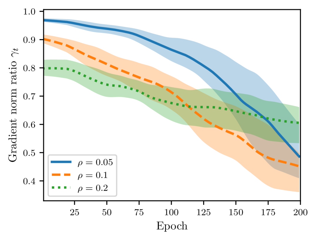
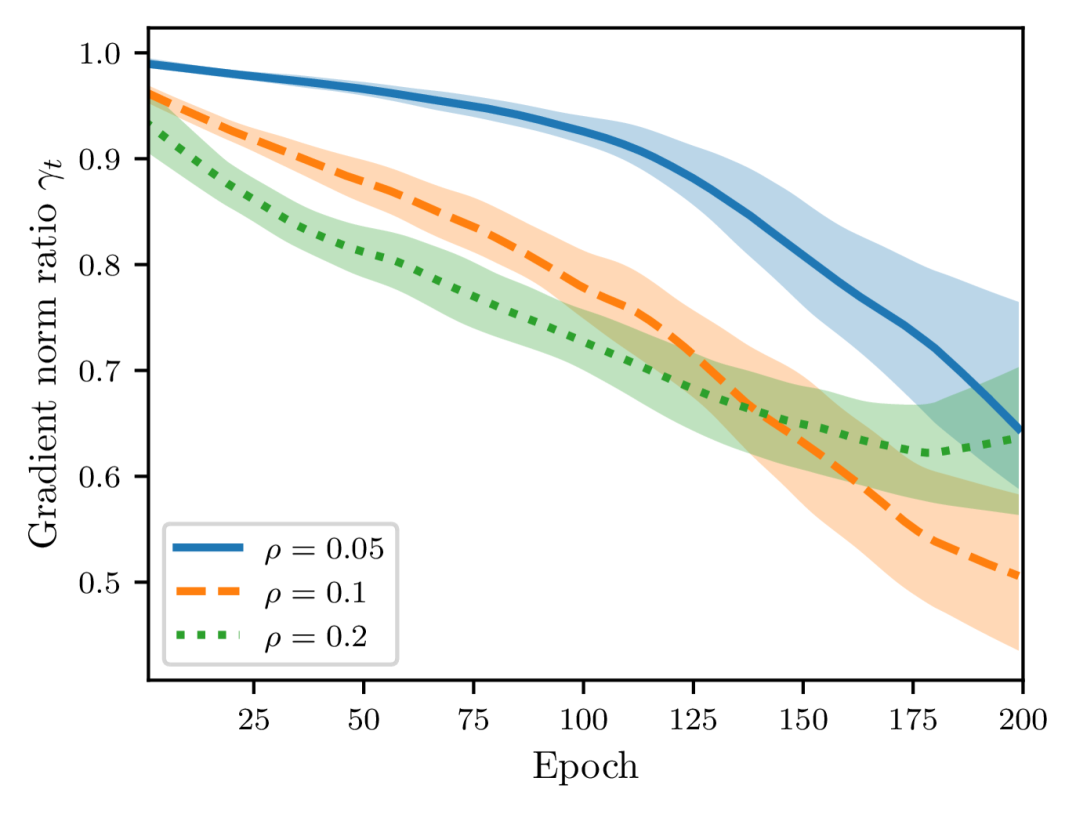
For a fixed perturbation radius $\rho$ , as shown in Figure 3, the renormalization factor $\gamma_{t}$ tends to decrease throughout training and is smaller than $1$ . Therefore, we can impose another assumption as follows.

Assumption 1

Suppose that there exist a constant $\gamma_{\mathrm{upp}}$ so that $\gamma_{t}$ is bounded for all $1\leq t\leq T$

0<\gamma_{t}\leq\gamma_{\mathrm{upp}}<1.

Notice that the constant $\gamma_{\mathrm{upp}}$ is not universal but problem-specific. Under this assumption, we can derive a similar growth rate of $\|\boldsymbol{v}_{t}-\boldsymbol{w}_{t}\|_{2}$ as Lemma 2.

Lemma 11

Let Assumption 1 hold and assume that the per-example loss function $f(\boldsymbol{w},z)$ is $\mu$ -strongly convex, $L$ -smooth and $G$ -Lipschitz continuous with respect to the first argument $\boldsymbol{w}$ . Suppose that at step $t$ , the examples selected by SSAM are the same in $S$ and $S^{\prime}$ and the corresponding update rules are denoted by $\boldsymbol{w}_{t+1}=\boldsymbol{w}_{t}-\eta\gamma_{t}\nabla f(\boldsymbol{w}_{t}^{asc},z)$ and $\boldsymbol{v}_{t+1}=\boldsymbol{v}_{t}-\eta\gamma_{t}\nabla f(\boldsymbol{v}_{t}^{asc},z)$ , respectively. Then, it follows that for all $1\leq t\leq T$

\|\boldsymbol{v}_{t+1}-\boldsymbol{w}_{t+1}\|_{2}\leq\left(1-\left(1+\mu\rho\right)\frac{\gamma_{t}\eta\mu L}{\mu+L}\right)\|\boldsymbol{v}_{t}-\boldsymbol{w}_{t}\|_{2},

(4)

where the learning rate $\eta$ satisfies that

\eta\leq\frac{1}{\gamma_{\mathrm{upp}}}\left[\frac{2}{\mu+L}-\frac{\mu+L}{2\mu L(\mu/\rho L^{2}+1)}\right].

(5)

Proof The proof is similar to Lemma 2. According to the update rule of SSAM, we have

	$\displaystyle\\|\boldsymbol{v}_{t+1}-\boldsymbol{w}_{t+1}\\|_{2}^{2}={}\\|\boldsymbol{v}_{t}-\gamma_{t}\eta\nabla f(\boldsymbol{v}_{t}^{asc})-\left(\boldsymbol{w}_{t}-\gamma_{t}\eta\nabla f(\boldsymbol{w}_{t}^{asc})\right)\\|_{2}^{2}$
	$\displaystyle{}={}\\|\boldsymbol{v}_{t}-\boldsymbol{w}_{t}\\|_{2}^{2}-2\gamma_{t}\eta\left<\boldsymbol{v}_{t}-\boldsymbol{w}_{t},\nabla f(\boldsymbol{v}_{t}^{asc})-\nabla f(\boldsymbol{w}_{t}^{asc})\right>+\gamma_{t}^{2}\eta^{2}\\|\nabla f(\boldsymbol{v}_{t}^{asc})-\nabla f(\boldsymbol{w}_{t}^{asc})\\|_{2}^{2}$
	$\displaystyle=\begin{aligned} &\\|\boldsymbol{v}_{t}-\boldsymbol{w}_{t}\\|_{2}^{2}-2\gamma_{t}\eta\left<\boldsymbol{v}_{t}^{asc}-\boldsymbol{w}_{t}^{asc},\nabla f(\boldsymbol{v}_{t}^{asc})-\nabla f(\boldsymbol{w}_{t}^{asc})\right>\\ &\quad+2\gamma_{t}\rho\eta\left<\nabla f(\boldsymbol{v}_{t})-\nabla f(\boldsymbol{w}_{t}),\nabla f(\boldsymbol{v}_{t}^{asc})-\nabla f(\boldsymbol{w}_{t}^{asc})\right>+\gamma_{t}^{2}\eta^{2}\\|\nabla f(\boldsymbol{v}_{t}^{asc})-\nabla f(\boldsymbol{w}_{t}^{asc})\\|_{2}^{2}\end{aligned}$
	$\displaystyle\stackrel{{\scriptstyle①}}{{\leq}}\begin{aligned} &\left(1-2\left(1+\mu\rho\right)\frac{\gamma_{t}\eta\mu L}{\mu+L}\right)\\|\boldsymbol{v}_{t}-\boldsymbol{w}_{t}\\|_{2}^{2}-2\left(\frac{\mu\rho}{L^{2}}+\rho^{2}\right)\frac{\gamma_{t}\eta\mu L}{\mu+L}\\|\nabla f(\boldsymbol{v}_{t})-\nabla f(\boldsymbol{w}_{t})\\|_{2}^{2}\\ &\quad+2\gamma_{t}\rho\eta\left<\nabla f(\boldsymbol{v}_{t})-\nabla f(\boldsymbol{w}_{t}),\nabla f(\boldsymbol{v}_{t}^{asc})-\nabla f(\boldsymbol{w}_{t}^{asc})\right>+\left(\gamma_{t}^{2}\eta^{2}-\frac{2\gamma_{t}\eta}{\mu+L}\right)\\|\nabla f(\boldsymbol{v}_{t}^{asc})-\nabla f(\boldsymbol{w}_{t}^{asc})\\|_{2}^{2}\end{aligned}$
	$\displaystyle\stackrel{{\scriptstyle②}}{{\leq}}\begin{aligned} &\left(1-2\left(1+\mu\rho\right)\frac{\gamma_{t}\eta\mu L}{\mu+L}\right)\\|\boldsymbol{v}_{t}-\boldsymbol{w}_{t}\\|_{2}^{2}+\left[\frac{\rho^{2}\gamma_{t}\eta}{\frac{2}{\mu+L}-\gamma_{t}\eta}-2\left(\frac{\mu\rho}{L^{2}}+\rho^{2}\right)\frac{\gamma_{t}\eta\mu L}{\mu+L}\right]\\|\nabla f(\boldsymbol{v}_{t})-\nabla f(\boldsymbol{w}_{t})\\|_{2}^{2}\\ &\quad+\left(\gamma_{t}^{2}\eta^{2}-\frac{2\gamma_{t}\eta}{\mu+L}\right)\left[\left(\nabla f\left(\boldsymbol{v}_{t}^{asc}\right)-\nabla f\left(\boldsymbol{w}_{t}^{asc}\right)\right)-\frac{\rho}{\frac{2}{\mu+L}-\gamma_{t}\eta}\left(\nabla f\left(\boldsymbol{v}_{t}\right)-\nabla f\left(\boldsymbol{w}_{t}\right)\right)\right]^{2}\end{aligned}$
	$\displaystyle\stackrel{{\scriptstyle③}}{{\leq}}{}\left(1-2\left(1+\mu\rho\right)\frac{\gamma_{t}\eta\mu L}{\mu+L}\right)\\|\boldsymbol{v}_{t}-\boldsymbol{w}_{t}\\|_{2}^{2},$

where $①$ is due to the coercivity of the loss function (cf. Appendix B) that

\left<\nabla f(\boldsymbol{v}_{t}^{asc})-\nabla f(\boldsymbol{w}_{t}^{asc}),\boldsymbol{v}_{t}^{asc}-\boldsymbol{w}_{t}^{asc}\right>\geq\frac{\mu L}{\mu+L}\|\boldsymbol{v}_{t}^{asc}-\boldsymbol{w}_{t}^{asc}\|_{2}^{2}+\frac{1}{\mu+L}\|\nabla f(\boldsymbol{v}_{t}^{asc})-\nabla f(\boldsymbol{w}_{t}^{asc})\|_{2}^{2}.

Moreover, ③ holds since the last two terms of ② are smaller than zero provided that the learning rate $\eta$ satisfies the given condition. Consequently, we have

\|\boldsymbol{v}_{t+1}-\boldsymbol{w}_{t+1}\|_{2}\leq\left(1-2\left(1+\mu\rho\right)\frac{\gamma_{t}\eta\mu L}{\mu+L}\right)^{1/2}\|\boldsymbol{v}_{t}-\boldsymbol{w}_{t}\|_{2}\leq\left(1-\left(1+\mu\rho\right)\frac{\gamma_{t}\eta\mu L}{\mu+L}\right)\|\boldsymbol{v}_{t}-\boldsymbol{w}_{t}\|_{2},

where the last inequality is due to the fact that $\sqrt{1-x}\leq 1-x/2$ holds for all $x\in[0,1]$ .
On the other hand, when the examples selected from $S$ and $S^{\prime}$ are different, we can obtain a similar result as Lemma 4.

Lemma 12

Assume the same settings as in Lemma 11. For the $t$ -th iteration, suppose that the examples selected by SSAM are different in $S$ and $S^{\prime}$ and that $\boldsymbol{w}_{t+1}=\boldsymbol{w}_{t}-\eta\gamma_{t}\nabla f(\boldsymbol{w}_{t}^{asc},z)$ and $\boldsymbol{v}_{t+1}=\boldsymbol{v}_{t}-\eta\gamma_{t}\nabla f(\boldsymbol{v}_{t}^{asc},z^{\prime})$ . Consequently, we obtain

\|\boldsymbol{v}_{t+1}-\boldsymbol{w}_{t+1}\|_{2}\leq\left(1-\left(1+\mu\rho\right)\frac{\gamma_{t}\eta\mu L}{\mu+L}\right)\|\boldsymbol{v}_{t}-\boldsymbol{w}_{t}\|_{2}+2\eta\gamma_{t}G.

Proof The proof is straightforward. It follows immediately from

	$\displaystyle\\|\boldsymbol{v}_{t+1}-\boldsymbol{w}_{t+1}\\|_{2}$	$\displaystyle=\\|\boldsymbol{v}_{t}-\eta\gamma_{t}\nabla f(\boldsymbol{v}_{t}^{asc},z^{\prime})-\left(\boldsymbol{w}_{t}-\eta\gamma_{t}\nabla f(\boldsymbol{v}_{t}^{asc},z^{\prime})\right)-\eta\gamma_{t}\left(\nabla f(\boldsymbol{v}_{t}^{asc},z^{\prime})-\nabla f(\boldsymbol{w}_{t}^{asc},z)\right)\\|_{2}$
		$\displaystyle\leq\\|\boldsymbol{v}_{t}-\eta\gamma_{t}\nabla f(\boldsymbol{v}_{t}^{asc},z^{\prime})-\left(\boldsymbol{w}_{t}-\eta\gamma_{t}\nabla f(\boldsymbol{v}_{t}^{asc},z^{\prime})\right)\\|_{2}+\eta\gamma_{t}\\|\nabla f(\boldsymbol{v}_{t}^{asc},z^{\prime})-\nabla f(\boldsymbol{w}_{t}^{asc},z)\\|_{2}$
		$\displaystyle\leq\left(1-\left(1+\mu\rho\right)\frac{\gamma_{t}\eta\mu L}{\mu+L}\right)\\|\boldsymbol{v}_{t}-\boldsymbol{w}_{t}\\|_{2}+2\eta\gamma_{t}G,$

thus concluding the proof.
With the above two lemmas, we can show that SSAM consistently performs better than SAM in terms of the generalization error. Before that, we need to introduce an auxiliary lemma as follows.

Lemma 13

Consider a sequence $\gamma_{1},\ldots,\gamma_{T}$ , where $0<\gamma_{k}<1$ for any $1\leq k\leq T$ . Denote the maximum of the first $k$ elements by $\gamma_{max}^{k}$ . Then, for any constants $\alpha>0$ , $0<\beta<1/\gamma_{max}^{T}$ , and $i=1,2,\ldots$ , the following inequality holds

\left(1-\gamma_{k+1}\beta\right)\Psi(k)+\left(\gamma_{k+1}\right)^{i}\alpha\leq\Psi(k+1),

where

\Psi(k)=\left[\left(1-\gamma_{max}^{k}\beta\right)^{k-1}+\ldots+\left(1-\gamma_{max}^{k}\beta\right)+1\right]\left(\gamma_{max}^{k}\right)^{i}\alpha.

Proof To prove this result, we only need to substitute $\Psi(k)$ in. In the case of $\gamma_{k+1}\geq\gamma_{max}^{k}$ , we have

		$\displaystyle\Psi(k+1)-\left(1-\gamma_{k+1}\beta\right)\Psi(k)-\left(\gamma_{k+1}\right)^{i}\alpha$
		$\displaystyle=\frac{\alpha}{\beta}\left(1-\gamma_{k+1}\beta\right)\left\{\left(\gamma_{k+1}\right)^{i-1}\left[1-\left(1-\gamma_{k+1}\beta\right)^{k}\right]-\left(\gamma_{max}^{k}\right)^{i-1}\left[1-\left(1-\gamma_{max}^{k}\beta\right)^{k}\right]\right\}\geq 0.$

In the case of $\gamma_{k+1}\leq\gamma_{max}^{k}$ , we also have

\displaystyle\Psi(k+1)-\left(1-\gamma_{k+1}\beta\right)\Psi(k)-\left(\gamma_{k+1}\right)^{i}\alpha\geq\alpha\gamma_{k+1}\left[\left(\gamma_{max}^{k}\right)^{i-1}-\left(\gamma_{k+1}\right)^{i-1}\right]\geq 0,

thus concluding the proof.

Theorem 14

Under assumptions and parameter settings in Lemmas 11 and 12. Suppose we run the SSAM iteration with constant learning rate $\eta$ satisfying (5) for $T$ steps. Then, SSAM satisfies uniform stability with

\varepsilon_{\mathrm{gen}}^{\mathrm{ssam}}\leq\frac{2G^{2}(\mu+L)}{n\mu L(1+\mu\rho)}\left\{1-\left[1-\left(1+\mu\rho\right)\frac{\gamma_{\mathrm{upp}}\eta\mu L}{\mu+L}\right]^{T}\right\}.

Proof Define $\delta_{t}=\|\boldsymbol{w}_{t}-\boldsymbol{v}_{t}\|_{2}$ to denote the Euclidean distance between $\boldsymbol{w}_{t}$ and $\boldsymbol{v}_{t}$ as training continues. Observe that at any step $t\leq T$ , with a probability $1-1/n$ , the selected examples from $S$ and $S^{\prime}$ are the same. In contrast, with a probability of $1/n$ , the selected examples are different. This is because $S$ and $S^{\prime}$ only differ by one example. Therefore, from Lemmas 11 and 12, we conclude that

	$\displaystyle\mathbb{E}[\delta_{t}]$	$\displaystyle\leq\left(1-\frac{1}{n}\right)\left(1-\left(1+\mu\rho\right)\frac{\gamma_{t}\eta\mu L}{\mu+L}\right)\mathbb{E}[\delta_{t-1}]+\frac{1}{n}\left(1-\left(1+\mu\rho\right)\frac{\gamma_{t}\eta\mu L}{\mu+L}\right)\mathbb{E}[\delta_{t-1}]+\frac{2\eta\gamma_{t}G}{n}$
		$\displaystyle=\left(1-\left(1+\mu\rho\right)\frac{\gamma_{t}\eta\mu L}{\mu+L}\right)\mathbb{E}[\delta_{t-1}]+\frac{2\eta\gamma_{t}G}{n}.$

Write $\beta=\eta\mu L\left(1+\mu\rho\right)/\left(\mu+L\right)$ and $\alpha=2\eta G/n$ , we then unravel the above recursion and obtain from Lemma 13 that

\mathbb{E}[\delta_{T}]\leq\gamma_{\mathrm{upp}}\alpha\sum_{t=0}^{T-1}\left(1-\gamma_{\mathrm{upp}}\beta\right)^{t}=\frac{2G(\mu+L)}{n\mu L(1+\mu\rho)}\left\{1-\left[1-\left(1+\mu\rho\right)\frac{\gamma_{\mathrm{upp}}\eta\mu L}{\mu+L}\right]^{T}\right\}.

Plugging this inequality into (1), we complete the proof.

Remark 15

Compared to SAM, this theorem indicates that the bound over generalization error can be further reduced by SSAM because the extra term $\gamma_{\mathrm{upp}}$ is smaller than $1$ .

4.3.2 Convergence

Similar to Theorem 8, we show that SSAM also converges to a noisy ball when the learning rate $\eta$ is fixed.

Theorem 16

Let Assumption 1 hold and suppose the loss function $f(\boldsymbol{w},z)$ is $\mu$ -strongly convex, $L$ -smooth, and $G$ -Lipschitz continuous with respect to the first argument $\boldsymbol{w}$ . Consider the sequence $\boldsymbol{w}_{0},\boldsymbol{w}_{1},\cdots,\boldsymbol{w}_{T}$ generated by running SSAM with a constant learning rate $\eta$ for $T$ steps. Let $\boldsymbol{w}^{*}\in\arg\inf_{\boldsymbol{w}}F_{S}(\boldsymbol{w})$ , it follows that

\displaystyle\varepsilon_{\mathrm{opt}}^{\mathrm{ssam}}=\mathbb{E}\left[F_{S}(\boldsymbol{w}_{T})-F_{S}(\boldsymbol{w}^{*})\right]\leq\left[1-\gamma_{\mathrm{upp}}\eta\mu\rho(\mu+L)\right]^{T}\mathbb{E}\left[F_{S}(\boldsymbol{w}_{0})-F_{S}(\boldsymbol{w}^{*})\right]+\frac{LG^{2}\left(\rho^{2}L+\gamma_{\mathrm{upp}}\eta\right)}{4\mu\rho(\mu+L)}.

Proof The proof follows the same steps as Theorem 10. From Taylor’s theorem, there exists a $\widehat{\boldsymbol{w}}_{t}$ such that

	$\displaystyle F_{S}(\boldsymbol{w}_{t+1})$	$\displaystyle=F_{S}\left(\boldsymbol{w}_{t}-\gamma_{t}\eta\nabla f(\boldsymbol{w}_{t}^{asc})\right)$
		$\displaystyle=F_{S}(\boldsymbol{w}_{t})-\gamma_{t}\eta\left<\nabla f(\boldsymbol{w}_{t}^{asc}),\nabla F_{S}(\boldsymbol{w}_{t})\right>+\frac{\gamma_{t}^{2}\eta^{2}}{2}\nabla f(\boldsymbol{w}_{t}^{asc})^{T}\nabla^{2}F_{S}(\widehat{\boldsymbol{w}}_{t})\nabla f(\boldsymbol{w}_{t}^{asc})$
		$\displaystyle\leq F_{S}(\boldsymbol{w}_{t})-\gamma_{t}\eta\left<\nabla f(\boldsymbol{w}_{t}^{asc}),\nabla F_{S}(\boldsymbol{w}_{t})\right>+\frac{\gamma_{t}^{2}\eta^{2}L}{2}\\|\nabla f(\boldsymbol{w}_{t}^{asc})\\|_{2}^{2}$
		$\displaystyle\leq F_{S}(\boldsymbol{w}_{t})-\gamma_{t}\eta\left<\nabla f(\boldsymbol{w}_{t}^{asc}),\nabla F_{S}(\boldsymbol{w}_{t})\right>+\frac{\gamma_{t}^{2}\eta^{2}LG^{2}}{2}.$

According to Lemma 7, it follows that

	$\displaystyle\mathbb{E}\left<\nabla f(\boldsymbol{w}_{t}^{asc}),\nabla F_{S}(\boldsymbol{w}_{t})\right>$	$\displaystyle\geq\rho(\mu+L)\left\\|\nabla F_{S}(\boldsymbol{w}_{t})\right\\|_{2}^{2}-\frac{\rho^{2}L^{2}G^{2}}{2}$
		$\displaystyle\geq 2\mu\rho(\mu+L)\left[F_{S}(\boldsymbol{w}_{t})-F_{S}(\boldsymbol{w}^{*})\right]-\frac{\rho^{2}L^{2}G^{2}}{2},$

\displaystyle\mathbb{E}\left[F_{S}(\boldsymbol{w}_{t+1})-F_{S}(\boldsymbol{w}^{*})\right]\leq\left[1-\gamma_{t}\eta\mu\rho(\mu+L)\right]\mathbb{E}\left[F_{S}(\boldsymbol{w}_{t})-F_{S}(\boldsymbol{w}^{*})\right]+\frac{\gamma_{t}\eta\rho^{2}L^{2}G^{2}}{2}+\frac{\gamma_{t}^{2}\eta^{2}G^{2}L}{2}.

Recursively applying Lemma 13 and summing up the geometric series yields

\displaystyle\mathbb{E}\left[F_{S}(\boldsymbol{w}_{T})-F_{S}(\boldsymbol{w}^{*})\right]\leq\left[1-\gamma_{\mathrm{upp}}\eta\mu\rho(\mu+L)\right]^{T}\mathbb{E}\left[F_{S}(\boldsymbol{w}_{0})-F_{S}(\boldsymbol{w}^{*})\right]+\frac{LG^{2}\left(\rho^{2}L+\gamma_{\mathrm{upp}}\eta\right)}{4\mu\rho(\mu+L)},

thus concluding the proof.

Remark 17

Since we require that $\gamma_{\mathrm{upp}}$ is smaller than $1$ , compared to SAM, this theorem suggests that SSAM nevertheless slows down the training process.

Combining these results, we can present an upper bound over the expected excess risk of the SSAM algorithm as follows.

Theorem 18

Under assumptions and parameter settings in Theorems 14 and 16, the expected excess risk $\varepsilon_{\mathrm{exc}}^{\mathrm{ssam}}$ of the output $\boldsymbol{w}_{T}$ obeys $\varepsilon_{\mathrm{exc}}^{\mathrm{ssam}}\leq\varepsilon_{\mathrm{opt}}^{\mathrm{ssam}}+\varepsilon_{\mathrm{gen}}^{\mathrm{ssam}}$ , where $\varepsilon_{\mathrm{opt}}^{\mathrm{ssam}}$ and $\varepsilon_{\mathrm{gen}}^{\mathrm{ssam}}$ are given by Theorems 14 and 16, respectively. Furthermore, as $T$ tends to infinity, we have

\varepsilon_{\mathrm{exc}}^{\mathrm{ssam}}\leq\frac{2G^{2}(\mu+L)}{n\mu L(1+\mu{\rho})}+\frac{LG^{2}\left(\rho^{2}L+\gamma_{\mathrm{upp}}\eta\right)}{4\mu\rho(\mu+L)}.

Proof This result follows immediately as $T\to\infty$ .

Remark 19

This theorem implies that SSAM would eventually achieve a tighter bound over the expected excess risk than SAM when the model is trained for a sufficiently long time.

5 Experiments

In this section, we present the empirical results on a range of tasks. From the perspective of algorithmic stability, we first investigate how SSAM ameliorates the issue of training instability with realistic data sets. We then provide the convergence results on a quadratic loss function. To demonstrate that the increased stability does not come at the cost of performance degradation, we also evaluate it on tasks such as training deep classifiers from scratch. The results suggest that SSAM can achieve comparable or even superior performance compared to SAM. For completeness, sometimes we also include the results of the standard formulation of SAM proposed by Foret et al. (2021) and denote it by $\mathrm{SAM}^{\ast}$ .

5.1 Algorithmic Stability

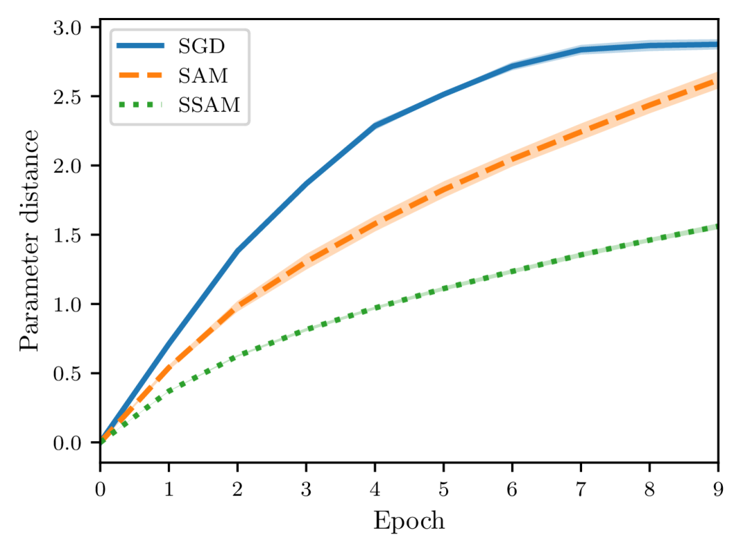
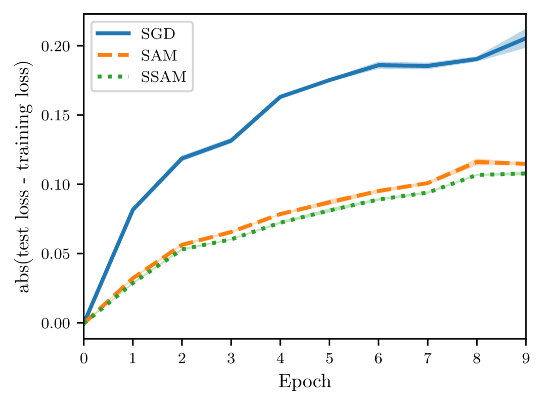
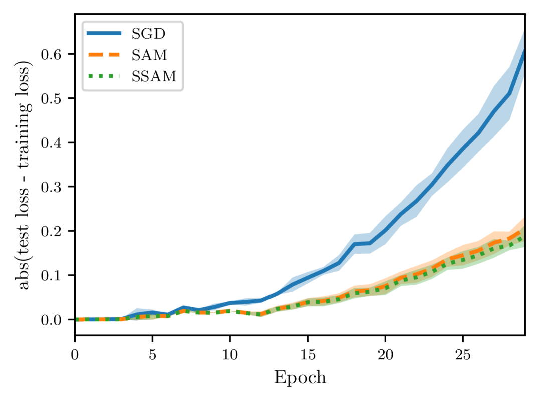
In Section 4.3, we showed that SSAM can consistently perform better than SAM in terms of generalization error (see Theorems 5 and 14 for a comparison). To verify this claim empirically, we follow the experimental settings of Hardt et al. (2016) and consider two proxies to measure the algorithmic stability. The first is the Euclidean distance between the parameters of two identical models, namely, with the same architecture and initialization. The second proxy is the generalization error which measures the difference between the training error and the test error.

To construct two training sets $S$ and $S^{\prime}$ that differ in only one example, we first randomly remove an example from the given training set, and the remaining examples naturally constitute one set $S$ . Then we can create another set $S^{\prime}$ by replacing a random example of $S$ with the one previously deleted. We restrict our attention to the task of image classification and adopt two different neural architectures: a simple fully connected neural network (FCN) trained on MNIST, and a LeNet (LeCun et al., 1998) trained on CIFAR-10. The FCN model consists of two hidden layers of 500 neurons, each of which is followed by a ReLU activation function. To make our experiments more controllable, we exclude all forms of regularization such as weight decay and dropout. We use the vanilla SGD (namely, mini-batch size is $1$ ) without momentum acceleration as the default base optimizer and train each model with a constant learning rate. Of course, we also fix the random seed at each epoch to ensure that the order of examples in two training sets remains the same. Additionally, we do not use data augmentation so that the distribution shift between training data and test data is minimal. Moreover, we record the Euclidean distance and the generalization error once per epoch.

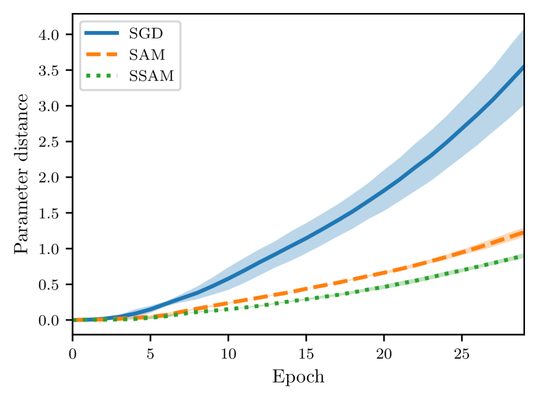
As shown in Figures 4 and 5, there is a close correspondence between the parameter distance and the generalization error. These two quantities often move in tandem and are positively correlated. Moreover, when starting from the same initialization, models trained by SGD quickly diverge, whereas models trained by SAM and SSAM change slowly. By comparing the training curves, we can further observe that SSAM is significantly less sensitive than SAM when the training set is modified.

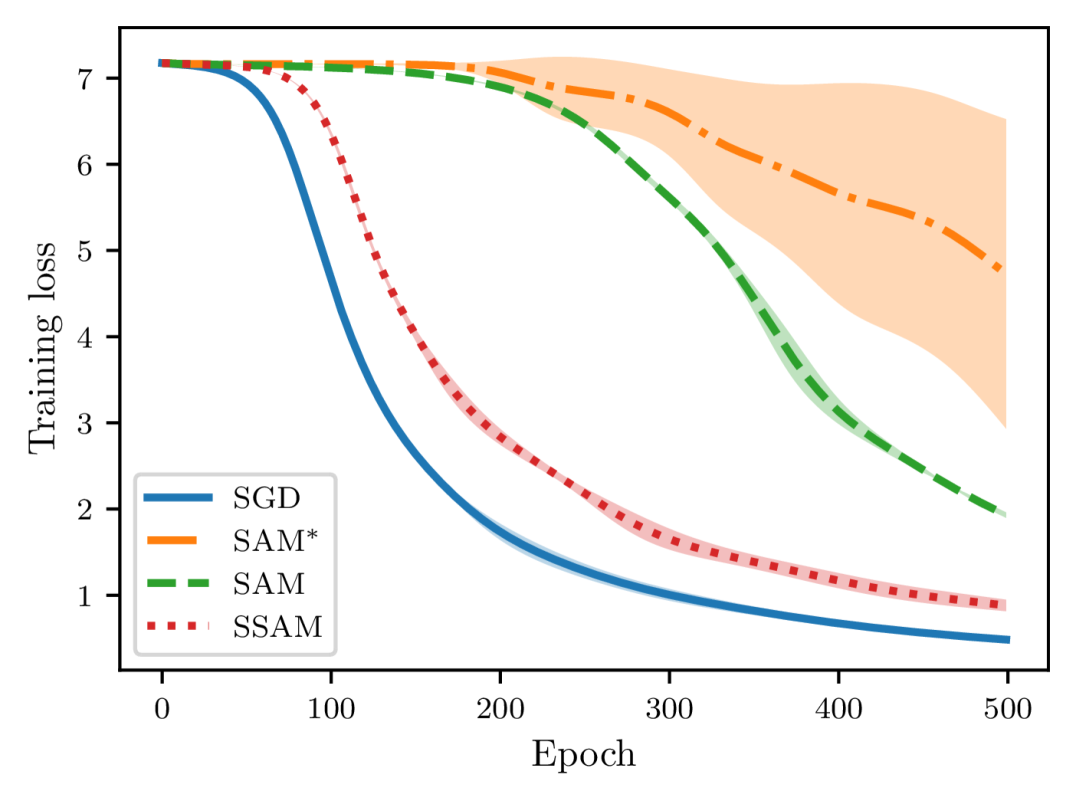
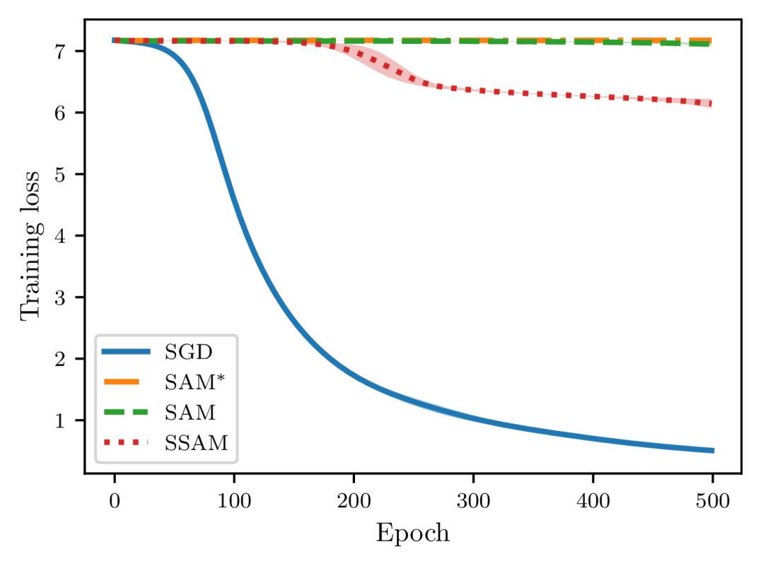
5.2 Convergence Results

To empirically validate the convergence results of SAM and SSAM, here we consider a quadratic loss function of dimension $d=20$ ,

f(x)=\frac{1}{2}x^{T}({AA^{T}}/{2d}+\delta\mathbb{I})x,

where $A\in\mathbb{R}^{d\times 2d}$ is a random matrix with elements being standard Gaussian noise and $\delta$ is a small positive coefficient to ensure that the loss function is strongly convex. Starting from a point sampled according to $\mathcal{N}(0,\mathbb{I})$ , we optimize the loss function for one million steps with a constant learning rate of $1.0e^{-3}$ . To introduce stochasticity, we also perturb the gradient at each step with random noise from $\mathcal{N}(0,1.0e^{-4})$ .

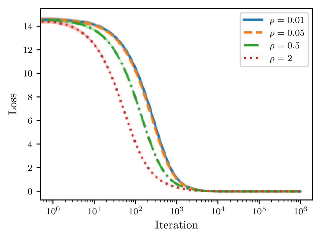
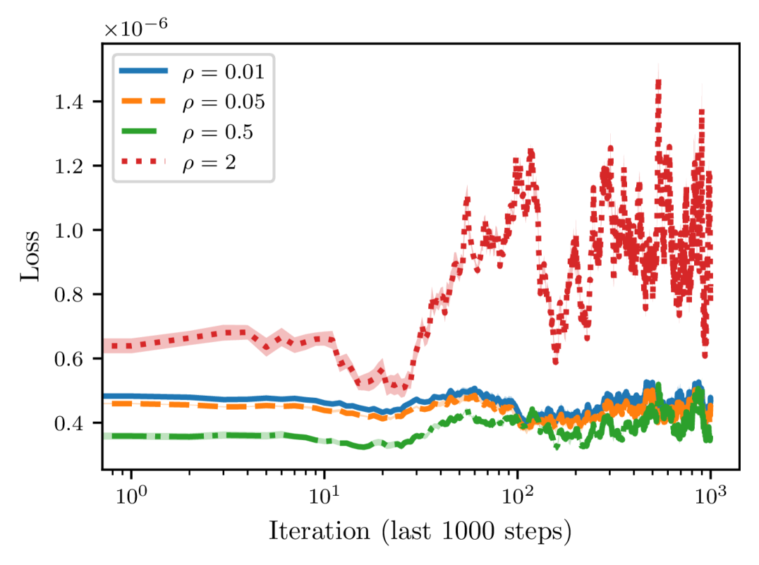
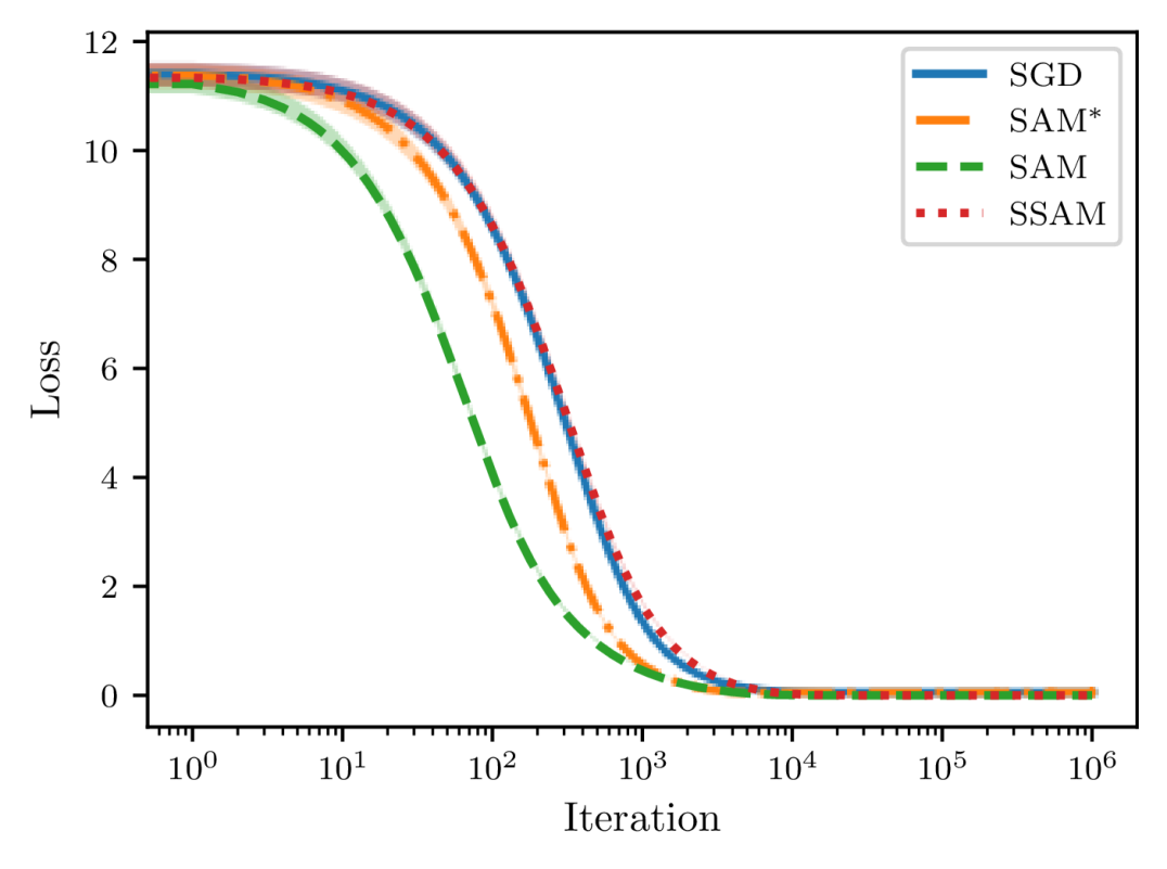
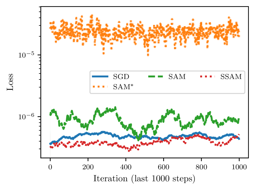
As depicted in Figure 6, we can observe that the convergence speed of SAM grows with the perturbation radius $\rho$ . More importantly, as we gradually increase $\rho$ from $0.01$ to $2$ , the loss at the end of training first decreases and then starts to increase, suggesting that there indeed exists a tradeoff between $\rho^{2}L$ and the learning rate $\eta$ as predicted by Theorem 8. We then compare SSAM against SAM and SGD in Figure 7 and find that SSAM indeed slows down the convergence speed. But, just as implied by Theorem 16, it is able to achieve a lower loss than SAM when trained for a sufficiently long period. Meanwhile, although SAM converges faster than SGD, it nevertheless converges to a larger noisy ball than SGD, which once again suggests that a careful choice of $\rho$ is critical to achieving a better generalization performance. From Figure 7(b), we can also observe that $\mathrm{SAM}^{\ast}$ seems to be more unstable than SAM because of the normalization step.

5.3 Image Classification from Scratch

We now continue to investigate how SSAM performs on real-world image classification problems. The baselines include SGD, SAM (Andriushchenko and Flammarion, 2022), $\mathrm{SAM}^{\ast}$ (Foret et al., 2021), ASAM (Kwon et al., 2021), and one-step GASAM (Zhang et al., 2022) that attempts to stabilize the training dynamics as well.

Table 1: Results on CIFAR-10 and CIFAR-100. We run each model with three different random seeds and report the mean test accuracy (%) along with the standard deviation. Text marked as bold indicates the best result.

ResNet-20 ResNet-56 ResNext-29-32x4d WRN-28-10 PyramidNet-110 CIFAR-10 SGD 92.78 $\pm$ 0.11 93.99 $\pm$ 0.19 95.47 $\pm$ 0.06 96.08 $\pm$ 0.16 96.02 $\pm$ 0.16 $\mathrm{SAM}^{\ast}$ 93.39 $\pm$ 0.14 94.93 $\pm$ 0.21 96.30 $\pm$ 0.01 96.91 $\pm$ 0.12 96.95 $\pm$ 0.06 SAM 93.43 $\pm$ 0.24 94.92 $\pm$ 0.22 96.20 $\pm$ 0.08 96.55 $\pm$ 0.17 96.91 $\pm$ 0.16 SSAM 93.46 $\pm$ 0.22 95.01 $\pm$ 0.19 96.33 $\pm$ 0.16 96.65 $\pm$ 0.18 97.04 $\pm$ 0.09 ASAM 93.11 $\pm$ 0.23 94.51 $\pm$ 0.34 95.74 $\pm$ 0.06 96.24 $\pm$ 0.08 96.39 $\pm$ 0.14 GASAM 92.96 $\pm$ 0.14 94.18 $\pm$ 0.31 93.66 $\pm$ 0.92 95.75 $\pm$ 0.34 81.83 $\pm$ 1.58 CIFAR-100 SGD 69.11 $\pm$ 0.11 72.38 $\pm$ 0.17 79.93 $\pm$ 0.15 80.42 $\pm$ 0.06 81.39 $\pm$ 0.31 $\mathrm{SAM}^{\ast}$ 70.30 $\pm$ 0.32 74.81 $\pm$ 0.07 81.09 $\pm$ 0.37 83.23 $\pm$ 0.19 84.03 $\pm$ 0.27 SAM 70.77 $\pm$ 0.24 75.02 $\pm$ 0.19 81.25 $\pm$ 0.14 82.94 $\pm$ 0.35 83.68 $\pm$ 0.10 SSAM 70.48 $\pm$ 0.18 75.11 $\pm$ 0.14 81.35 $\pm$ 0.13 82.80 $\pm$ 0.15 83.78 $\pm$ 0.17 ASAM 69.57 $\pm$ 0.12 72.82 $\pm$ 0.32 80.01 $\pm$ 0.14 81.34 $\pm$ 0.31 82.04 $\pm$ 0.09 GASAM 69.02 $\pm$ 0.13 72.05 $\pm$ 1.09 77.81 $\pm$ 1.52 81.48 $\pm$ 0.31 45.59 $\pm$ 3.03

CIFAR-10 and CIFAR-100. Here we adopt several popular backbones, ranging from basic ResNets (He et al., 2016) to more advanced architectures such as WideResNet (Zagoruyko and Komodakis, 2016), ResNeXt (Xie et al., 2017), and PyramidNet (Han et al., 2017). To increase reproductivity, we decide to employ the standard implementations of these architectures that are encapsulated in a Pytorch package⁴⁴4Details can be found at https://pypi.org/project/pytorchcv.. Beyond the training and test set, we also construct a validation set containing 5000 images out of the training set. Moreover, we only employ basic data augmentations such as horizontal flip, random crop, and normalization. We set the mini-batch size to be 128 and each model is trained up to 200 epochs with a cosine learning rate decay (Loshchilov and Hutter, 2016). The default base optimizer is SGD with a momentum of 0.9. To determine the best choice of hyper-parameters for each backbone, slightly different from Kwon et al. (2021); Kim et al. (2022), we first use SGD to grid search the learning rate and the weight decay coefficient over {0.01, 0.05, 0.1} and {1.0e-4, 5.0e-4, 1.0e-3}, respectively. For SAM and the variants, these two hyper-parameters are then fixed. As suggested by Kwon et al. (2021), the perturbation radius $\rho$ of ASAM needs to be much larger, and we thus range it from {0.5, 1.0, 2.0}. In contrast, we sweep the perturbation radius $\rho$ of other optimizers over {0.05, 0.1, 0.2}. We run each model with three different random seeds and report the mean and the standard deviation of the accuracy on the test set.

As shown in Table 1, apart from GASAM that even fails to converge for PyramidNet-110, both SAM and its variants are able to consistently perform better than the base optimizer SGD. Meanwhile, it is worth noting that there is no significant difference between SAM (Andriushchenko and Flammarion, 2022) and $\mathrm{SAM}^{\ast}$ (Foret et al., 2021), suggesting that the normalization term is not necessary for promoting generalization performance. Focusing on the rows of SSAM and SAM, we further observe that SSAM can achieve a higher test accuracy than SAM on most backbones, though the improvements may not be significant.

ImageNet-1K (Deng et al., 2009). To investigate the performance of the renormalization strategy on a larger scale, we further evaluate it with the ImageNet-1K data set. We only employ basic data augmentations, namely, resizing and cropping images to 224-pixel resolution and then normalizing them. We adopt several typical architectures⁵⁵5Both models are trained with the timm library that is available at https://github.com/huggingface/pytorch-image-models., including two ResNets (ResNet-18/50), and two vision transformers (ViT-S-16/32) (Dosovitskiy et al., 2021). ResNet-18 and ResNet-50 are trained for 90 and 100 epochs, respectively. The default base optimizer is SGD with momentum acceleration, the peak learning rate is 0.1, and the weight decay coefficient is 1.0e-4. According to Foret et al. (2021), the perturbation radius $\rho$ is set to be 0.05. For the vision transformer, the two models are trained up to 300 epochs and the default base optimizer is switched to AdamW. The peak learning rate is 3.0e-4 and the weight decay coefficient is 0.3. The value of $\rho$ is 0.2 because the vision transformer favors larger $\rho$ than ResNet does (Chen et al., 2022). For both models, we use a constant mini-batch size of 256, and the cosine learning rate decay schedule is also employed. As shown in Table 2, the renormalization strategy remains effective on the ImageNet-1K data set. After applying the renormalization strategy to SAM, we can observe an improved top-1 accuracy on the validation set for all models, though the improvement is more pronounced for the two vision transformers.

Table 2: Top-1 accuracy (%) on ImageNet-1K validation set with Inception-style data augmentation only. The base optimizer for ResNet is SGD with a momentum of 0.9. In contrast, the base optimizer for the vision transformer is AdamW.

SGD/AdamW $\mathrm{SAM}^{\ast}$ SAM SSAM ResNet-18 70.56 $\pm$ 0.03 70.74 $\pm$ 0.02 70.66 $\pm$ 0.12 70.76 $\pm$ 0.09 ResNet-50 77.09 $\pm$ 0.12 77.81 $\pm$ 0.04 77.82 $\pm$ 0.08 77.89 $\pm$ 0.13 ViT-S-32 65.42 $\pm$ 0.12 67.42 $\pm$ 0.21 69.98 $\pm$ 0.11 71.15 $\pm$ 0.18 ViT-S-16 72.25 $\pm$ 0.09 73.81 $\pm$ 0.06 76.88 $\pm$ 0.25 77.41 $\pm$ 0.13

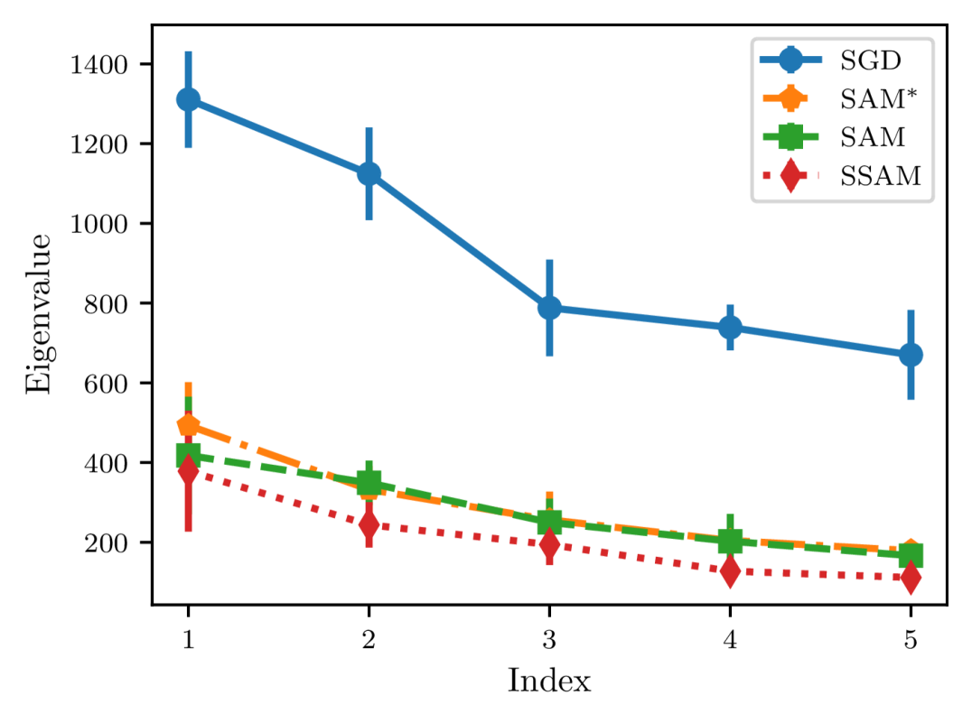
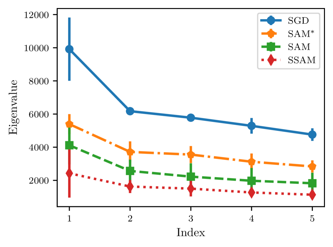
5.4 Minima Analysis

Finally, to gain a better understanding of SSAM, we further compare the differences in the sharpness of the minima found by different optimizers, which can be described by the dominant eigenvalue of the Hessian of the loss function (Foret et al., 2021; Zhuang et al., 2022; Kaddour et al., 2022). For this purpose, we train a ResNet-20 on CIFAR-10 and a ResNet-56 on CIFAR-100 using the same hyper-parameters and then estimate the top five eigenvalues of the Hessian.

From Figure 8, we can observe that compared to SGD, SAM significantly reduces the sharpness of the minima. Meanwhile, it also can be observed that SSAM achieves the lowest eigenvalue, suggesting that the renormalization strategy is indeed beneficial in escaping saddle points and finding flatter regions of the loss landscape.

6 Conclusion

In this paper, we proposed a renormalization strategy to mitigate the issue of instability in sharpness-aware training. We also evaluated its efficacy, both theoretically and empirically. Following this line, we believe several directions deserve further investigation. Although we have verified that SSAM and SAM both can greatly improve the generalization performance over SGD, it remains unknown whether they converge to the same attractor of minima, properties of which might significantly differ from those found by SGD (Kaddour et al., 2022). Moreover, probing to what extent the renormalization strategy reshapes the optimization trajectory or the parameter space it explores is also of interest. Another intriguing direction involves controlling the renormalization factor during the training process, for example, by imposing explicit constraints on its bounds or adjusting the perturbation radius according to the gradient norm of the ascent step. Finally, the influence of renormalization strategy on adversarial robustness should also be investigated (Wei et al., 2023).

Acknowledgments

This work is supported in part by the National Key Research and Development Program of China under Grant 2020AAA0105601, in part by the National Natural Science Foundation of China under Grants 12371512 and 62276208, and in part by the Natural Science Basic Research Program of Shaanxi Province 2024JC-JCQN-02.

A Training Instability on Realistic Neural Networks

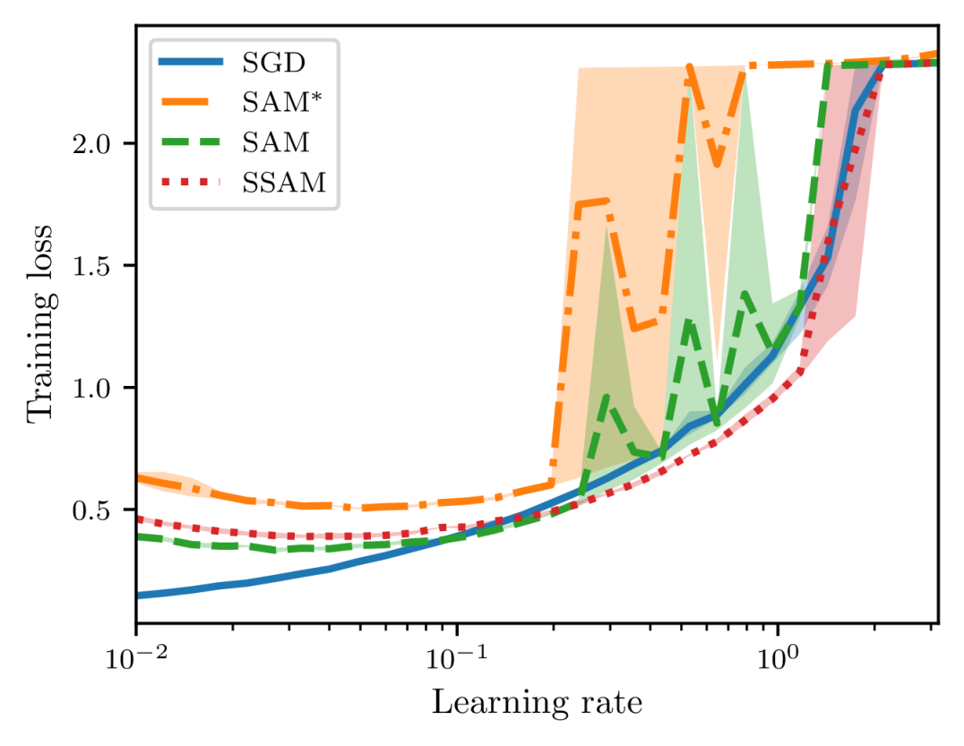
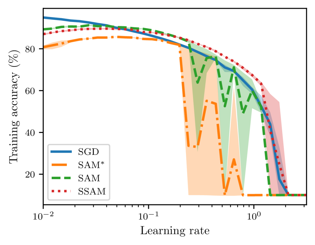
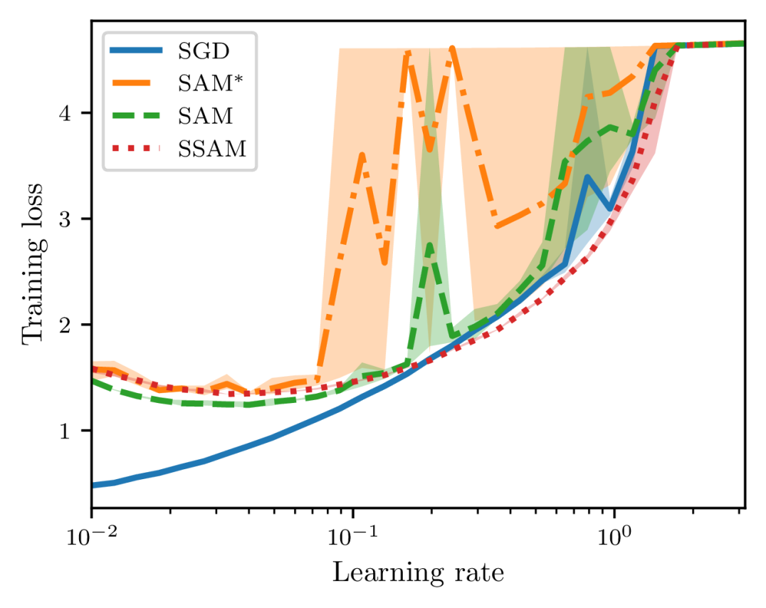
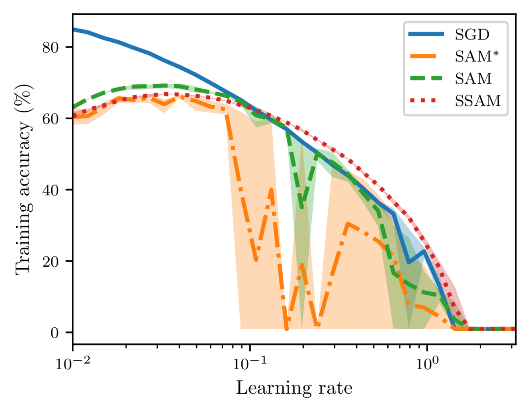
To examine the training stability on real-world applications, we also train a ResNet-20 on CIFAR-10 and a ResNet-56 on CIFAR-100 with different learning rates that are equispaced between 0.01 and 3.16 on the logarithm scale. The default optimizer is SGD with a mini-batch size of $128$ and each model is trained up to $200$ epochs. To make the difference more significant, we use a relatively large value of $\rho=1.0$ , and the learning rate is not decayed throughout training.

In Figures 9 and 10, we report the metrics of loss and accuracy on the training set at the end of training. When the learning rate is small, we can observe that SGD attains the lowest loss and SAM performs better than SSAM. As we continue to increase the learning rate, however, SAM becomes highly unstable and finally fails to converge. As a comparison, we can observe that SSAM is more stable than SAM and even can achieve a lower loss and a higher accuracy than SGD in a relatively large range of learning rates. Notice that SAM^∗ is still much more unstable than SAM because of the normalization step.

B Coercivity of Strongly Convex Function

Lemma 20

A function $f(\boldsymbol{w}):\mathbb{R}^{d}\mapsto\mathbb{R}_{+}$ is $\mu$ -strongly convex and $L$ -smooth, for all $\boldsymbol{w}$ , $\boldsymbol{v}\in\mathbb{R}^{d}$ , we have

\left<\nabla f(\boldsymbol{v})-\nabla f(\boldsymbol{w}),\boldsymbol{v}-\boldsymbol{w}\right>\geq\frac{\mu L}{\mu+L}\|\boldsymbol{v}-\boldsymbol{w}\|_{2}^{2}+\frac{1}{\mu+L}\|\nabla f(\boldsymbol{v})-\nabla f(\boldsymbol{w})\|_{2}^{2}.

Proof Consider the function $\varphi(\boldsymbol{w})=f(\boldsymbol{w})-\frac{\mu}{2}\|\boldsymbol{w}\|_{2}^{2}$ , which is convex with $(L-\mu)$ -smooth by appealing to the fact that $f(\boldsymbol{w})$ is $\mu$ -strongly convex and $L$ -smooth. Therefore, it follows that

\left<\nabla\varphi(\boldsymbol{v})-\nabla\varphi(\boldsymbol{w}),\boldsymbol{v}-\boldsymbol{w}\right>\geq\frac{1}{L-\mu}\|\nabla\varphi(\boldsymbol{v})-\nabla\varphi(\boldsymbol{w})\|_{2}^{2}.

On the other hand,

\left<\nabla\varphi(\boldsymbol{v})-\nabla\varphi(\boldsymbol{w}),\boldsymbol{v}-\boldsymbol{w}\right>=\left<\nabla f(\boldsymbol{v})-\nabla f(\boldsymbol{w}),\boldsymbol{v}-\boldsymbol{w}\right>-\mu\left<\boldsymbol{v}-\boldsymbol{w},\boldsymbol{v}-\boldsymbol{w}\right>.

Substituting the preceding inequality in, we have

\displaystyle\left<\nabla f(\boldsymbol{v})-\nabla f(\boldsymbol{w}),\boldsymbol{v}-\boldsymbol{w}\right>

\displaystyle\geq\frac{1}{L-\mu}\|\nabla f(\boldsymbol{v})-\nabla f(\boldsymbol{w})-\mu(\boldsymbol{v}-\boldsymbol{w})\|_{2}^{2}+\mu\|\boldsymbol{v}-\boldsymbol{w}\|_{2}^{2}.

Expanding the first term on the right side, it follows that

\left<\nabla f(\boldsymbol{v})-\nabla f(\boldsymbol{w}),\boldsymbol{v}-\boldsymbol{w}\right>\geq\frac{\mu L}{\mu+L}\|\boldsymbol{v}-\boldsymbol{w}\|_{2}^{2}+\frac{1}{\mu+L}\|\nabla f(\boldsymbol{v})-\nabla f(\boldsymbol{w})\|_{2}^{2},

thus concluding the proof.

References

Andriushchenko and Flammarion (2022) Maksym Andriushchenko and Nicolas Flammarion. Towards understanding sharpness-aware minimization. In Proceedings of the 43rd International Conference on Machine Learning, pages 639–668, 2022.
Bahri et al. (2022) Dara Bahri, Hossein Mobahi, and Yi Tay. Sharpness-aware minimization improves language model generalization. In Proceedings of the 60th Annual Meeting of the Association for Computational Linguistics, volume 1, pages 7360–7371, 2022.
Bartlett et al. (2023) Peter L Bartlett, Philip M Long, and Olivier Bousquet. The dynamics of sharpness-aware minimization: Bouncing across ravines and drifting towards wide minima. Journal of Machine Learning Research, 24(316):1–36, 2023.
Bisla et al. (2022) Devansh Bisla, Jing Wang, and Anna Choromanska. Low-pass filtering SGD for recovering flat optima in the deep learning optimization landscape. In Proceedings of the 25th International Conference on Artificial Intelligence and Statistics, pages 8299–8339, 2022.
Bottou et al. (2018) Léon Bottou, Frank E Curtis, and Jorge Nocedal. Optimization methods for large-scale machine learning. SIAM Review, 60(2):223–311, 2018.
Bousquet and Elisseeff (2002) Olivier Bousquet and André Elisseeff. Stability and generalization. The Journal of Machine Learning Research, 2:499–526, 2002.
Bubeck et al. (2015) Sébastien Bubeck et al. Convex optimization: Algorithms and complexity. Foundations and Trends® in Machine Learning, 8(3-4):231–357, 2015.
Chaudhari et al. (2019) Pratik Chaudhari, Anna Choromanska, Stefano Soatto, Yann LeCun, Carlo Baldassi, Christian Borgs, Jennifer Chayes, Levent Sagun, and Riccardo Zecchina. Entropy-SGD: Biasing gradient descent into wide valleys. Journal of Statistical Mechanics: Theory and Experiment, 2019(12):124018, 2019.
Chen et al. (2022) Xiangning Chen, Cho-Jui Hsieh, and Boqing Gong. When vision Transformers outperform Resnets without pretraining or strong data augmentations. In Proceedings of the 10th International Conference on Learning Representations, pages 1–20, 2022.
Choi et al. (2019) Dami Choi, Christopher J Shallue, Zachary Nado, Jaehoon Lee, Chris J Maddison, and George E Dahl. On empirical comparisons of optimizers for deep learning. arXiv preprint arXiv:1910.05446, 2019.
Compagnoni et al. (2023) Enea Monzio Compagnoni, Luca Biggio, Antonio Orvieto, Frank Norbert Proske, Hans Kersting, and Aurelien Lucchi. An SDE for modeling SAM: Theory and insights. In Proceedings of the 44th International Conference on Machine Learning, pages 25209–25253, 2023.
Dahl et al. (2023) George E Dahl, Frank Schneider, Zachary Nado, Naman Agarwal, Chandramouli Shama Sastry, Philipp Hennig, Sourabh Medapati, Runa Eschenhagen, Priya Kasimbeg, Daniel Suo, et al. Benchmarking neural network training algorithms. arXiv preprint arXiv:2306.07179, 2023.
Dai et al. (2024) Yan Dai, Kwangjun Ahn, and Suvrit Sra. The crucial role of normalization in sharpness-aware minimization. In Proceedings of 37th Conference on Neural Information Processing Systems, pages 1–13, 2024.
Dai et al. (2019) Zihang Dai, Zhilin Yang, Yiming Yang, Jaime G Carbonell, Quoc Le, and Ruslan Salakhutdinov. Transformer-XL: Attentive language models beyond a fixed-length context. In Proceedings of the 57th Annual Meeting of the Association for Computational Linguistics, pages 2978–2988, 2019.
Davies et al. (2021) Alex Davies, Petar Veličković, Lars Buesing, Sam Blackwell, Daniel Zheng, Nenad Tomašev, Richard Tanburn, Peter Battaglia, Charles Blundell, András Juhász, et al. Advancing mathematics by guiding human intuition with AI. Nature, 600(7887):70–74, 2021.
Deng et al. (2009) Jia Deng, Wei Dong, Richard Socher, Li-Jia Li, Kai Li, and Li Fei-Fei. Imagenet: A large-scale hierarchical image database. In Proceedings of the 25th IEEE/CVF Conference on Computer Vision and Pattern Recognition, pages 248–255, 2009.
Dinh et al. (2017) Laurent Dinh, Razvan Pascanu, Samy Bengio, and Yoshua Bengio. Sharp minima can generalize for deep nets. In Proceedings of the 34th International Conference on Machine Learning, pages 1019–1028, 2017.
Dosovitskiy et al. (2021) Alexey Dosovitskiy, Lucas Beyer, Alexander Kolesnikov, Dirk Weissenborn, Xiaohua Zhai, Thomas Unterthiner, Mostafa Dehghani, Matthias Minderer, Georg Heigold, Sylvain Gelly, et al. An image is worth 16x16 words: Transformers for image recognition at scale. In Proceedings of the International Conference on Learning Representations, pages 1–21, 2021.
Du et al. (2022a) Jiawei Du, Hanshu Yan, Jiashi Feng, Joey Tianyi Zhou, Liangli Zhen, Rick Siow Mong Goh, and Vincent Tan. Efficient sharpness-aware minimization for improved training of neural networks. In Proceedings of the 10th International Conference on Learning Representations, pages 1–18, 2022a.
Du et al. (2022b) Jiawei Du, Daquan Zhou, Jiashi Feng, Vincent Tan, and Joey Tianyi Zhou. Sharpness-aware training for free. In Proceedings of the 36th Conference on Neural Information Processing Systems, volume 35, pages 23439–23451, 2022b.
Du et al. (2017) Simon S Du, Chi Jin, Jason D Lee, Michael I Jordan, Aarti Singh, and Barnabas Poczos. Gradient descent can take exponential time to escape saddle points. In Proceedings of 31st Conference on Neural Information Processing Systems, pages 1–19, 2017.
Duchi et al. (2011) John Duchi, Elad Hazan, and Yoram Singer. Adaptive subgradient methods for online learning and stochastic optimization. Journal of Machine Learning Research, 12(7), 2011.
Foret et al. (2021) Pierre Foret, Ariel Kleiner, Hossein Mobahi, and Behnam Neyshabur. Sharpness-aware minimization for efficiently improving generalization. In Proceedings of the 9th International Conference on Learning Representations, pages 1–20, 2021.
Han et al. (2017) Dongyoon Han, Jiwhan Kim, and Junmo Kim. Deep pyramidal residual networks. In Proceedings of the 33rd IEEE/CVF Conference on Computer Vision and Pattern Recognition, pages 5927–5935, 2017.
Hardt et al. (2016) Moritz Hardt, Ben Recht, and Yoram Singer. Train faster, generalize better: Stability of stochastic gradient descent. In Proceedings of the 37th International Conference on Machine Learning, pages 1225–1234, 2016.
Haruki et al. (2019) Kosuke Haruki, Taiji Suzuki, Yohei Hamakawa, Takeshi Toda, Ryuji Sakai, Masahiro Ozawa, and Mitsuhiro Kimura. Gradient noise convolution: Smoothing loss function for distributed large-batch SGD. arXiv preprint arXiv:1906.10822, 2019.
He et al. (2019) Fengxiang He, Tongliang Liu, and Dacheng Tao. Control batch size and learning rate to generalize well: Theoretical and empirical evidence. In Proceedings of 33rd Conference on Neural Information Processing Systems, volume 32, pages 1–10, 2019.
He et al. (2016) Kaiming He, Xiangyu Zhang, Shaoqing Ren, and Jian Sun. Deep residual learning for image recognition. In Proceedings of the 32nd IEEE Conference on Computer Vision and Pattern Recognition, pages 770–778, 2016.
Hinton and van Camp (1993) Geoffrey E Hinton and Drew van Camp. Keeping neural networks simple. In Proceedings of the International Conference on Artificial Neural Networks, pages 11–18, 1993.
Jastrzębski et al. (2018) Stanisław Jastrzębski, Zachary Kenton, Devansh Arpit, Nicolas Ballas, Asja Fischer, Yoshua Bengio, and Amos Storkey. Three factors influencing minima in SGD. Artificial Neural Networks and Machine Learning, pages 1–14, 2018.
Jastrzebski et al. (2021) Stanislaw Jastrzebski, Devansh Arpit, Oliver Astrand, Giancarlo B Kerg, Huan Wang, Caiming Xiong, Richard Socher, Kyunghyun Cho, and Krzysztof J Geras. Catastrophic Fisher explosion: Early phase fisher matrix impacts generalization. In Proceedings of the 38th International Conference on Machine Learning, pages 4772–4784, 2021.
Jiang et al. (2023) Weisen Jiang, Hansi Yang, Yu Zhang, and James Kwok. An adaptive policy to employ sharpness-aware minimization. In Proceedings of the 11st International Conference on Learning Representations, pages 1–19, 2023.
Jiang et al. (2020) Yiding Jiang, Behnam Neyshabur, Hossein Mobahi, Dilip Krishnan, and Samy Bengio. Fantastic generalization measures and where to find them. In Proceedings of the 8th International Conference on Learning Representations, pages 1–33, 2020.
Jumper et al. (2021) John Jumper, Richard Evans, Alexander Pritzel, Tim Green, Michael Figurnov, Olaf Ronneberger, Kathryn Tunyasuvunakool, Russ Bates, Augustin Žídek, Anna Potapenko, et al. Highly accurate protein structure prediction with AlphaFold. Nature, 596(7873):583–589, 2021.
Kaddour et al. (2022) Jean Kaddour, Linqing Liu, Ricardo Silva, and Matt J Kusner. When do flat minima optimizers work? In Proceedings of the 36th Conference on Neural Information Processing Systems, volume 35, pages 16577–16595, 2022.
Keskar et al. (2017) Nitish Shirish Keskar, Dheevatsa Mudigere, Jorge Nocedal, Mikhail Smelyanskiy, and Ping Tak Peter Tang. On large-batch training for deep learning: Generalization gap and sharp minima. In Proceedings of the 5th International Conference on Learning Representations, pages 1–16, 2017.
Kim et al. (2023) Hoki Kim, Jinseong Park, Yujin Choi, and Jaewook Lee. Stability analysis of sharpness-aware minimization. arXiv preprint arXiv:2301.06308, 2023.
Kim et al. (2022) Minyoung Kim, Da Li, Shell X Hu, and Timothy Hospedales. Fisher SAM: Information geometry and sharpness aware minimisation. In Proceedings of the 43rd International Conference on Machine Learning, pages 11148–11161, 2022.
Kingma and Ba (2014) Diederik P Kingma and Jimmy Ba. Adam: A method for stochastic optimization. arXiv preprint arXiv:1412.6980, 2014.
Kleinberg et al. (2018) Bobby Kleinberg, Yuanzhi Li, and Yang Yuan. An alternative view: When does SGD escape local minima? In Proceedings of the 35th International Conference on Machine Learning, pages 2698–2707, 2018.
Kunin et al. (2019) Daniel Kunin, Jonathan Bloom, Aleksandrina Goeva, and Cotton Seed. Loss landscapes of regularized linear autoencoders. In Proceedings of the 36th International Conference on Machine Learning, pages 3560–3569, 2019.
Kwon et al. (2021) Jungmin Kwon, Jeongseop Kim, Hyunseo Park, and In Kwon Choi. ASAM: Adaptive sharpness-aware minimization for scale-invariant learning of deep neural networks. In Proceedings of the 42nd International Conference on Machine Learning, pages 5905–5914, 2021.
LeCun et al. (1998) Yann LeCun, Léon Bottou, Yoshua Bengio, and Patrick Haffner. Gradient-based learning applied to document recognition. Proceedings of the IEEE, 86(11):2278–2324, 1998.
Liu et al. (2022a) Yong Liu, Siqi Mai, Xiangning Chen, Cho-Jui Hsieh, and Yang You. Towards efficient and scalable sharpness-aware minimization. In Proceedings of the 38th IEEE/CVF Conference on Computer Vision and Pattern Recognition, pages 12360–12370, 2022a.
Liu et al. (2022b) Yong Liu, Siqi Mai, Minhao Cheng, Xiangning Chen, Cho-Jui Hsieh, and Yang You. Random sharpness-aware minimization. In Proceedings of the 36th Conference on Neural Information Processing Systems, volume 35, pages 24543–24556, 2022b.
Long and Bartlett (2024) Philip M Long and Peter L Bartlett. Sharpness-aware minimization and the edge of stability. Journal of Machine Learning Research, 25(179):1–20, 2024.
Loshchilov and Hutter (2016) Ilya Loshchilov and Frank Hutter. SGDR: Stochastic gradient descent with warm restarts. arXiv preprint arXiv:1608.03983, 2016.
Lucchi et al. (2021) Aurelien Lucchi, Antonio Orvieto, and Adamos Solomou. On the second-order convergence properties of random search methods. In Proceedings of the 35th Conference on Neural Information Processing Systems, volume 34, pages 25633–25645, 2021.
Mi et al. (2022) Peng Mi, Li Shen, Tianhe Ren, Yiyi Zhou, Xiaoshuai Sun, Rongrong Ji, and Dacheng Tao. Make sharpness-aware minimization stronger: A sparsified perturbation approach. In Proceedings of the 36th Conference on Neural Information Processing Systems, volume 35, pages 30950–30962, 2022.
Ni et al. (2022) Renkun Ni, Ping-yeh Chiang, Jonas Geiping, Micah Goldblum, Andrew Gordon Wilson, and Tom Goldstein. K-SAM: Sharpness-aware minimization at the speed of SGD. arXiv preprint arXiv:2210.12864, 2022.
Redmon et al. (2016) Joseph Redmon, Santosh Divvala, Ross Girshick, and Ali Farhadi. You only look once: Unified, real-time object detection. In Proceedings of the 31st IEEE/CVF Conference on Computer Vision and Pattern Recognition, pages 779–788, 2016.
Tan et al. (2024) Chengli Tan, Jiangshe Zhang, Junmin Liu, and Yihong Gong. Sharpness-aware Lookahead for accelerating convergence and improving generalization. IEEE Transactions on Pattern Analysis and Machine Intelligence, pages 1–14, 2024.
Wei et al. (2023) Zeming Wei, Jingyu Zhu, and Yihao Zhang. Sharpness-aware minimization alone can improve adversarial robustness. In New Frontiers in Adversarial Machine Learning Workshop of the 40th International Conference on Machine Learning, pages 1–12, 2023.
Wen et al. (2022) Kaiyue Wen, Tengyu Ma, and Zhiyuan Li. How does sharpness-aware minimization minimizes sharpness? In Optimization for Machine Learning Workshop of 35th Conference on Neural Information Processing Systems, pages 1–94, 2022.
Wen et al. (2024) Kaiyue Wen, Zhiyuan Li, and Tengyu Ma. Sharpness minimization algorithms do not only minimize sharpness to achieve better generalization. In Proceedings of 38th Conference on Neural Information Processing Systems, pages 1–12, 2024.
Wilson et al. (2017) Ashia C Wilson, Rebecca Roelofs, Mitchell Stern, Nati Srebro, and Benjamin Recht. The marginal value of adaptive gradient methods in machine learning. In Proceedings of 31st Conference on Neural Information Processing Systems, volume 30, pages 1–10, 2017.
Xie et al. (2017) Saining Xie, Ross Girshick, Piotr Dollár, Zhuowen Tu, and Kaiming He. Aggregated residual transformations for deep neural networks. In Proceedings of the 33rd IEEE/CVF Conference on Computer Vision and Pattern Recognition, pages 1492–1500, 2017.
Yao et al. (2020) Zhewei Yao, Amir Gholami, Kurt Keutzer, and Michael W Mahoney. Pyhessian: Neural networks through the lens of the Hessian. In Proceedings of the IEEE International Conference on Big Data, pages 581–590, 2020.
Yue et al. (2023) Yun Yue, Jiadi Jiang, Zhiling Ye, Ning Gao, Yongchao Liu, and Ke Zhang. Sharpness-aware minimization revisited: Weighted sharpness as a regularization term. In Proceedings of the 29th ACM SIGKDD Conference on Knowledge Discovery and Data Mining, pages 1–10, 2023.
Zagoruyko and Komodakis (2016) Sergey Zagoruyko and Nikos Komodakis. Wide residual networks. arXiv preprint arXiv:1605.07146, 2016.
Zhang et al. (2022) Zhiyuan Zhang, Ruixuan Luo, Qi Su, and Xu Sun. GA-SAM: Gradient-strength based adaptive sharpness-aware minimization for improved generalization. In Proceedings of the Conference on Empirical Methods in Natural Language Processing, pages 3888–3903, 2022.
Zhao et al. (2022a) Yang Zhao, Hao Zhang, and Xiuyuan Hu. Penalizing gradient norm for efficiently improving generalization in deep learning. In Proceedings of the 43rd International Conference on Machine Learning, pages 26982–26992, 2022a.
Zhao et al. (2022b) Yang Zhao, Hao Zhang, and Xiuyuan Hu. Randomized sharpness-aware training for boosting computational efficiency in deep learning. arXiv preprint arXiv:2203.09962, 2022b.
Zhou et al. (2020) Pan Zhou, Jiashi Feng, Chao Ma, Caiming Xiong, Steven Chu Hong Hoi, et al. Towards theoretically understanding why SGD generalizes better than Adam in deep learning. In Proceedings of 34th Conference on Neural Information Processing Systems, volume 33, pages 21285–21296, 2020.
Zhou et al. (2022) Wenxuan Zhou, Fangyu Liu, Huan Zhang, and Muhao Chen. Sharpness-aware minimization with dynamic reweighting. In Findings of the Association for Computational Linguistics, pages 5686–5699, 2022.
Zhuang et al. (2022) Juntang Zhuang, Boqing Gong, Liangzhe Yuan, Yin Cui, Hartwig Adam, Nicha C Dvornek, James s Duncan, Ting Liu, et al. Surrogate gap minimization improves sharpness-aware training. In Proceedings of the 10th International Conference on Learning Representations, pages 1–24, 2022.

	$\displaystyle\\|\boldsymbol{v}_{t}^{asc}-\boldsymbol{w}_{t}^{asc}\\|_{2}^{2}$	$\displaystyle=\\|\boldsymbol{v}_{t}-\boldsymbol{w}_{t}\\|_{2}^{2}+2\rho\left<\boldsymbol{v}_{t}-\boldsymbol{w}_{t},\nabla f(\boldsymbol{v}_{t})-\nabla f(\boldsymbol{w}_{t})\right>+\rho^{2}\\|\nabla f(\boldsymbol{v}_{t})-\nabla f(\boldsymbol{w}_{t})\\|_{2}^{2}$
		$\displaystyle\geq(1+2\mu\rho)\\|\boldsymbol{v}_{t}-\boldsymbol{w}_{t}\\|_{2}^{2}+\rho^{2}\\|\nabla f(\boldsymbol{v}_{t})-\nabla f(\boldsymbol{w}_{t})\\|_{2}^{2}$
		$\displaystyle\geq(1+\mu\rho)\\|\boldsymbol{v}_{t}-\boldsymbol{w}_{t}\\|_{2}^{2}+({\mu\rho}/{L^{2}}+\rho^{2})\\|\nabla f(\boldsymbol{v}_{t})-\nabla f(\boldsymbol{w}_{t})\\|_{2}^{2}.$

	$\displaystyle\\|\boldsymbol{v}_{t+1}-\boldsymbol{w}_{t+1}\\|_{2}^{2}={}\\|\boldsymbol{v}_{t}-\eta\nabla f(\boldsymbol{v}_{t}^{asc})-\left(\boldsymbol{w}_{t}-\eta\nabla f(\boldsymbol{w}_{t}^{asc})\right)\\|_{2}^{2}$
	$\displaystyle{}={}\\|\boldsymbol{v}_{t}-\boldsymbol{w}_{t}\\|_{2}^{2}-2\eta\left<\boldsymbol{v}_{t}-\boldsymbol{w}_{t},\nabla f(\boldsymbol{v}_{t}^{asc})-\nabla f(\boldsymbol{w}_{t}^{asc})\right>+\eta^{2}\\|\nabla f(\boldsymbol{v}_{t}^{asc})-\nabla f(\boldsymbol{w}_{t}^{asc})\\|_{2}^{2}$
	$\displaystyle=\begin{aligned} &\\|\boldsymbol{v}_{t}-\boldsymbol{w}_{t}\\|_{2}^{2}-2\eta\left<\boldsymbol{v}_{t}^{asc}-\boldsymbol{w}_{t}^{asc},\nabla f(\boldsymbol{v}_{t}^{asc})-\nabla f(\boldsymbol{w}_{t}^{asc})\right>\\ &\quad+2\rho\eta\left<\nabla f(\boldsymbol{v}_{t})-\nabla f(\boldsymbol{w}_{t}),\nabla f(\boldsymbol{v}_{t}^{asc})-\nabla f(\boldsymbol{w}_{t}^{asc})\right>+\eta^{2}\\|\nabla f(\boldsymbol{v}_{t}^{asc})-\nabla f(\boldsymbol{w}_{t}^{asc})\\|_{2}^{2}\end{aligned}$
	$\displaystyle\stackrel{{\scriptstyle①}}{{\leq}}\begin{aligned} &\left(1-2\left(1+\mu\rho\right)\frac{\eta\mu L}{\mu+L}\right)\\|\boldsymbol{v}_{t}-\boldsymbol{w}_{t}\\|_{2}^{2}-2\left(\frac{\mu\rho}{L^{2}}+\rho^{2}\right)\frac{\eta\mu L}{\mu+L}\\|\nabla f(\boldsymbol{v}_{t})-\nabla f(\boldsymbol{w}_{t})\\|_{2}^{2}\\ &\quad+2\rho\eta\left<\nabla f(\boldsymbol{v}_{t})-\nabla f(\boldsymbol{w}_{t}),\nabla f(\boldsymbol{v}_{t}^{asc})-\nabla f(\boldsymbol{w}_{t}^{asc})\right>+\left(\eta^{2}-\frac{2\eta}{\mu+L}\right)\\|\nabla f(\boldsymbol{v}_{t}^{asc})-\nabla f(\boldsymbol{w}_{t}^{asc})\\|_{2}^{2}\end{aligned}$
	$\displaystyle\stackrel{{\scriptstyle②}}{{\leq}}\begin{aligned} &\left(1-2\left(1+\mu\rho\right)\frac{\eta\mu L}{\mu+L}\right)\\|\boldsymbol{v}_{t}-\boldsymbol{w}_{t}\\|_{2}^{2}+\left[\frac{\rho^{2}\eta}{\frac{2}{\mu+L}-\eta}-2\left(\frac{\mu\rho}{L^{2}}+\rho^{2}\right)\frac{\eta\mu L}{\mu+L}\right]\\|\nabla f(\boldsymbol{v}_{t})-\nabla f(\boldsymbol{w}_{t})\\|_{2}^{2}\\ &\quad+\left(\eta^{2}-\frac{2\eta}{\mu+L}\right)\left[\left(\nabla f\left(\boldsymbol{v}_{t}^{asc}\right)-\nabla f\left(\boldsymbol{w}_{t}^{asc}\right)\right)-\frac{\rho}{\frac{2}{\mu+L}-\eta}\left(\nabla f\left(\boldsymbol{v}_{t}\right)-\nabla f\left(\boldsymbol{w}_{t}\right)\right)\right]^{2}\end{aligned}$
	$\displaystyle\stackrel{{\scriptstyle③}}{{\leq}}{}\left(1-2\left(1+\mu\rho\right)\frac{\eta\mu L}{\mu+L}\right)\\|\boldsymbol{v}_{t}-\boldsymbol{w}_{t}\\|_{2}^{2},$

	$\displaystyle\\|\boldsymbol{v}_{t+1}-\boldsymbol{w}_{t+1}\\|_{2}$	$\displaystyle=\\|\boldsymbol{v}_{t}-\eta\nabla f(\boldsymbol{v}_{t}^{asc},z^{\prime})-\left(\boldsymbol{w}_{t}-\eta\nabla f(\boldsymbol{w}_{t}^{asc},z^{\prime})\right)-\eta\left(\nabla f(\boldsymbol{w}_{t}^{asc},z^{\prime})-\nabla f(\boldsymbol{w}_{t}^{asc},z)\right)\\|_{2}$
		$\displaystyle\leq\\|\boldsymbol{v}_{t}-\eta\nabla f(\boldsymbol{v}_{t}^{asc},z^{\prime})-\left(\boldsymbol{w}_{t}-\eta\nabla f(\boldsymbol{w}_{t}^{asc},z^{\prime})\right)\\|_{2}+\eta\\|\nabla f(\boldsymbol{w}_{t}^{asc},z^{\prime})-\nabla f(\boldsymbol{w}_{t}^{asc},z)\\|_{2}$
		$\displaystyle\leq\left(1-\left(1+\mu\rho\right)\frac{\eta\mu L}{\mu+L}\right)\\|\boldsymbol{v}_{t}-\boldsymbol{w}_{t}\\|_{2}+2\eta G,$

	$\displaystyle\mathbb{E}\left<\nabla f(\widehat{\boldsymbol{w}}_{t}^{asc}),\nabla F_{S}(\boldsymbol{w}_{t})\right>$	$\displaystyle=\left<\nabla F_{S}(\widehat{\boldsymbol{w}}_{t}^{asc}),\nabla F_{S}(\boldsymbol{w}_{t})\right>$
		$\displaystyle=\left<\nabla F_{S}(\widehat{\boldsymbol{w}}_{t}^{asc})-\nabla F_{S}(\boldsymbol{w}_{t}),\nabla F_{S}(\boldsymbol{w}_{t})\right>+\left\\|\nabla F_{S}(\boldsymbol{w}_{t})\right\\|_{2}^{2}$
		$\displaystyle=\frac{1}{\rho}\left<\nabla F_{S}(\boldsymbol{w}+\rho\nabla F_{S}(\boldsymbol{w}_{t}))-\nabla F_{S}(\boldsymbol{w}_{t}),\rho\nabla F_{S}(\boldsymbol{w}_{t})\right>+\left\\|\nabla F_{S}(\boldsymbol{w}_{t})\right\\|_{2}^{2}$
		$\displaystyle\geq\left(1+\mu\rho\right)\left\\|\nabla F_{S}(\boldsymbol{w}_{t})\right\\|_{2}^{2}.$

	$\displaystyle\\|\boldsymbol{v}_{t+1}-\boldsymbol{w}_{t+1}\\|_{2}^{2}={}\\|\boldsymbol{v}_{t}-\gamma_{t}\eta\nabla f(\boldsymbol{v}_{t}^{asc})-\left(\boldsymbol{w}_{t}-\gamma_{t}\eta\nabla f(\boldsymbol{w}_{t}^{asc})\right)\\|_{2}^{2}$
	$\displaystyle{}={}\\|\boldsymbol{v}_{t}-\boldsymbol{w}_{t}\\|_{2}^{2}-2\gamma_{t}\eta\left<\boldsymbol{v}_{t}-\boldsymbol{w}_{t},\nabla f(\boldsymbol{v}_{t}^{asc})-\nabla f(\boldsymbol{w}_{t}^{asc})\right>+\gamma_{t}^{2}\eta^{2}\\|\nabla f(\boldsymbol{v}_{t}^{asc})-\nabla f(\boldsymbol{w}_{t}^{asc})\\|_{2}^{2}$
	$\displaystyle=\begin{aligned} &\\|\boldsymbol{v}_{t}-\boldsymbol{w}_{t}\\|_{2}^{2}-2\gamma_{t}\eta\left<\boldsymbol{v}_{t}^{asc}-\boldsymbol{w}_{t}^{asc},\nabla f(\boldsymbol{v}_{t}^{asc})-\nabla f(\boldsymbol{w}_{t}^{asc})\right>\\ &\quad+2\gamma_{t}\rho\eta\left<\nabla f(\boldsymbol{v}_{t})-\nabla f(\boldsymbol{w}_{t}),\nabla f(\boldsymbol{v}_{t}^{asc})-\nabla f(\boldsymbol{w}_{t}^{asc})\right>+\gamma_{t}^{2}\eta^{2}\\|\nabla f(\boldsymbol{v}_{t}^{asc})-\nabla f(\boldsymbol{w}_{t}^{asc})\\|_{2}^{2}\end{aligned}$
	$\displaystyle\stackrel{{\scriptstyle①}}{{\leq}}\begin{aligned} &\left(1-2\left(1+\mu\rho\right)\frac{\gamma_{t}\eta\mu L}{\mu+L}\right)\\|\boldsymbol{v}_{t}-\boldsymbol{w}_{t}\\|_{2}^{2}-2\left(\frac{\mu\rho}{L^{2}}+\rho^{2}\right)\frac{\gamma_{t}\eta\mu L}{\mu+L}\\|\nabla f(\boldsymbol{v}_{t})-\nabla f(\boldsymbol{w}_{t})\\|_{2}^{2}\\ &\quad+2\gamma_{t}\rho\eta\left<\nabla f(\boldsymbol{v}_{t})-\nabla f(\boldsymbol{w}_{t}),\nabla f(\boldsymbol{v}_{t}^{asc})-\nabla f(\boldsymbol{w}_{t}^{asc})\right>+\left(\gamma_{t}^{2}\eta^{2}-\frac{2\gamma_{t}\eta}{\mu+L}\right)\\|\nabla f(\boldsymbol{v}_{t}^{asc})-\nabla f(\boldsymbol{w}_{t}^{asc})\\|_{2}^{2}\end{aligned}$
	$\displaystyle\stackrel{{\scriptstyle②}}{{\leq}}\begin{aligned} &\left(1-2\left(1+\mu\rho\right)\frac{\gamma_{t}\eta\mu L}{\mu+L}\right)\\|\boldsymbol{v}_{t}-\boldsymbol{w}_{t}\\|_{2}^{2}+\left[\frac{\rho^{2}\gamma_{t}\eta}{\frac{2}{\mu+L}-\gamma_{t}\eta}-2\left(\frac{\mu\rho}{L^{2}}+\rho^{2}\right)\frac{\gamma_{t}\eta\mu L}{\mu+L}\right]\\|\nabla f(\boldsymbol{v}_{t})-\nabla f(\boldsymbol{w}_{t})\\|_{2}^{2}\\ &\quad+\left(\gamma_{t}^{2}\eta^{2}-\frac{2\gamma_{t}\eta}{\mu+L}\right)\left[\left(\nabla f\left(\boldsymbol{v}_{t}^{asc}\right)-\nabla f\left(\boldsymbol{w}_{t}^{asc}\right)\right)-\frac{\rho}{\frac{2}{\mu+L}-\gamma_{t}\eta}\left(\nabla f\left(\boldsymbol{v}_{t}\right)-\nabla f\left(\boldsymbol{w}_{t}\right)\right)\right]^{2}\end{aligned}$
	$\displaystyle\stackrel{{\scriptstyle③}}{{\leq}}{}\left(1-2\left(1+\mu\rho\right)\frac{\gamma_{t}\eta\mu L}{\mu+L}\right)\\|\boldsymbol{v}_{t}-\boldsymbol{w}_{t}\\|_{2}^{2},$

Stabilizing Sharpness-aware Minimization Through A Simple Renormalization Strategy

Abstract

1 Introduction

2 Related Works

3 Methodology

4 Theoretical Analysis

4.1 Notations and Preliminaries

Theorem 1 (Generalization error under ε\varepsilon-uniformly stability)

4.2 Expected Excess Risk Analysis of SAM

4.2.1 Stability

Lemma 2

Remark 3

Lemma 4

Theorem 5

Corollary 6

4.2.2 Convergence

Lemma 7

Theorem 8

Remark 9

Theorem 10

4.3 Expected Excess Risk Analysis of SSAM

4.3.1 Stability

Assumption 1

Lemma 11

Lemma 12

Lemma 13

Theorem 14

Remark 15

4.3.2 Convergence

Theorem 16

Remark 17

Theorem 18

Remark 19

5 Experiments

5.1 Algorithmic Stability

5.2 Convergence Results

5.3 Image Classification from Scratch

5.4 Minima Analysis

6 Conclusion

A Training Instability on Realistic Neural Networks

B Coercivity of Strongly Convex Function

Lemma 20

References

Theorem 1 (Generalization error under $\varepsilon$ -uniformly stability)