Stable massless scalar polarization of gravity
Abstract
Polarization is a prominent feature of gravitational wave observation, and it can be used to distinguish different modified gravities. Compared to General Relativity, gravity has an additional polarization coming from scalar field, which is a mix of the longitudinal and the breathing modes. When the scalar mass of is zero, the mixed mode will reduce to a pure breathing mode with the disappearance of the longitudinal mode. However, the reducing seems not to be allowed because a positive scalar mass is often needed to maintain the stability of the cosmological perturbation. In fact, the massless case is possible to lead to a stable perturbation, but more detailed constraints need to be considered. For the completeness of the polarization analysis, we explore the possibility that there is a stable massless scalar polarization in viable models for dark energy. We find that the existence of the massless scalar polarization depends not only on the number of free parameters but also on the model structure.
I Introduction
All kinds of cosmological observations have indicated that our Universe is expanding at an accelerating rate [1, 2, 3]. In order to explain the accelerating expansion, there are two main solutions: introducing dark energy and modifying Einstein’s General Relativity [4]. The latter corresponds to the modified gravity theories, which include theory [5, 6], Brans-Dicke theory [7, 8], scalar-tensor theory [9, 10] and so on. For theory, its way to modify General Relativity is to change the Ricci scalar in the Einstein-Hilbert action into an arbitrary function of , namely . When the field equations are derived from the action in gravity, two formalisms need to be distinguished. The first is the metric formalism, where the connections are set to be metric dependent. The second is the Palatini formalism [11], where the metric and the connections are assumed to be independent of each other. In this paper, viable dark energy models will be studied in the metric formalism.
Gravitational waves have been successfully observed [12, 13], and more and more gravitational-wave events are expected to be detected with the development of various gravitational wave detectors [14, 15, 16]. Therefore, it is possible to test different models of modified gravity according to the observations of gravitational waves. One of the most significant properties of gravitational waves is the polarization, which can be applied to test gravity theories effectively [17, 18, 19]. General Relativity has two independent polarizations coming from tensor field, while general four-dimensional modified gravity theories have up to six independent polarizations [17]. There are various methods for polarization analysis, mainly including geodesic deviation [20, 21], Newman-Penrose formalism [17, 22], extended Newman-Penrose formalism [23] and gauge invariants [24, 25, 26]. In the following section, geodesic deviation will be used to analyze polarizations.
For gravity, its propagating degree of freedom is three, and it has an additional polarization coming from scalar field besides the two same tensor polarizations as General Relativity [21]. The scalar polarization of is a mix of the longitudinal and the breathing modes, and the longitudinal mode will disappear when the scalar mass of is zero [21]. In other words, the massless scalar polarization of is a pure breathing mode rather than a mixed mode [27]. However, a positive value of scalar mass is often required to maintain the stability of the cosmological perturbation [28, 29], so that the massless case should seemingly be removed. In fact, the massless case is possible to lead to a stable perturbation, but more detailed constraints need to be considered [30]. In order to building a complete polarization analysis for gravity, it is necessary for us to give these detailed constraints and reexplore the possibility of existence of stable massless scalar polarization in gravity.
It is interesting to note that the massless scalar polarization is allowed to appear in the scalar-tensor theory [26] and the Brans-Dicke theory [31], but gravity, which is largely equivalent to the formers [32, 33], rarely has the massless scalar polarization. This inconsistency also prompts us to study the massless scalar polarization of gravity. Although relevant examples have been researched in [27, 34], some problems remain unresolved. In [27], a special power law model is considered, but it lacks the main features of viable models. In [34], the massless scalar polarization is given by directly setting the scalar mass to zero, but more detailed constraints for a stable perturbation are not involved, so that the de sitter point in the picture of effective potential might be an inflection point or a local maximum point instead of an expected local minimum point.
Our paper is organized as follows: in section II, we introduce the polarizations of general gravity and three viable models for dark energy. Particularly, the expression of scalar mass of is given. In section III, necessary constraints for stable massless scalar polarization are shown, and they come from the requirements of cosmology and effective potential. In section IV, the updated constraints are used to retest viable models whether they can reflect stable massless scalar polarization. In section V, discussions and conclusions are made. In this paper, the geometrized units are employed.
II Polarizations and gravity
In this section, we are going to introduce the gravitational wave polarizations of gravity and the specific models of viable individually. The polarization analysis will focus on a particular model () for a simple process, because the results of general model are similar to that of the particular model but require more complex calculations.
II.1 General results of polarizations
The action of gravity is as follows:
| (1) |
where , is the Ricci scalar, is an arbitrary function of , and is the matter action. In order to study gravitational wave in the absence of matter, we let for the vacuum field. In the metric formalism, the vacuum field equation of eq. (1) is obtained by varying its action:
| (2) |
where and . Taking the trace of eq. (2), we have:
| (3) |
For gravity, its de Sitter stage corresponds to a vacuum solution with a positive constant background curvature [29]. By perturbing eq. (3) with the de Sitter background curvature , the wave equation for the scalar field can be yielded:
| (4) |
Here the de Sitter stage is viewed as homogeneous and static, and is defined as:
| (5) |
According to [35], should meet the following condition:
| (6) |
At the scale size of gravitational wave detectors, the background metric can be nearly approximated to the Minkowski metric [26, 29]. Adding a perturbation to the background metric, one has:
| (7) |
where and is the Minkowski metric. From here on, the subsequent discussion is based on the particular model () for the simplicity of process [21]. A new tensor is introduced:
| (8) |
Following [21], the transverse traceless gauge conditions are allowed to use:
| (9) |
Combining eqs. (7), (8) and (9), the Ricci tensor under the perturbation of the metric becomes:
| (10) |
For the particular model , under the first-order perturbation of the metric, eq. (2) becomes:
| (11) |
Comparing eq. (10) with eq. (11), one gets:
| (12) |
where is obtained from eq. (5) for . According to eq. (3) and , one has and eq. (12) can be reduced to:
| (13) |
which is the wave equation for the tensor field. Eq. (13) is consistent with the wave equation of General Relativity, and it means that their tensor polarizations are the same (including the plus and the cross modes) [36]. Moreover, general model will also lead to the same tensor polarizations, see [29] for more details.
The scalar polarization in gravity is an extra polarization that General Relativity does not have, and let us start with the wave equation eq. (4) for the scalar field. For the plane wave traveling along the direction, the solution to eq. (4) is:
| (14) |
where is the complex conjugation, is the amplitude, and [21, 36]. Keep to remove the tensor part of eq. (8) and can be rewritten as the function of :
| (15) |
where . The following linear approximation is applied:
| (16) |
Bring eq. (15) into eq. (16) to obtain:
| (17) |
and hence the geodesic deviation can be turned into:
| (18) |
| (19) |
| (20) |
where for the particular model , eqs. (18) and (19) together stand for the breathing mode, and eq. (20) represents the longitudinal mode. It is shown that the scalar polarization of is a mix of the longitudinal and the breathing modes [21]. And the mixed mode will be reduced to a pure breathing mode when the scalar mass of (defined in eq. (5)) vanishes. Although the above discussions are nearly based on the particular model , some similar results have been given in general gravity [26] and even in other extended gravity theories which includes gravity [25, 26].
II.2 Specific models of gravity
In order to explore the possibility of massless scalar polarization in gravity, we are going to discuss several specific viable models including Hu-Sawicki [37], Starobinsky [38] and Gogoi-Dev [34]:
| (21) |
| (22) |
| (23) |
where is the inverse function of , and () are positive dimensionless parameters, while is a parameter in unit of curvature and roughly corresponds to the order of present Ricci scalar [6]. These above models are proposed for constructing viable dark energy models, and they all satisfy two assumptions: and as [38]. Here is the traditional CDM model, is the effective cosmological constant, and is considered to be unrelated to the quantum vacuum energy in above models [38]. Moreover, it should be noted that only 3-parameter models are involved. This is because that the subsequent constraints in section III will contain three independent equations and the models with 2 parameters or less should be naturally excluded.
In the following part, we will first show a series of substitutions and calculation results for the simplification of the subsequent processes. Let us make the following definitions:
| (24) |
| (25) |
| (26) |
where . It is worth noting that because the scalar mass in eq. (5) is defined by , the following stability conditions almost based on instead of . According to eq. (25) and eq. (26), ones have:
| (27) |
| (28) |
| (29) |
| (30) |
where , , and the same goes for higher derivatives. An agreement is made in our follow-up parts: the object of derivation depends on what the variable is in the parentheses behind the function. Besides, when the variable is changed to a specific value with a subscript ‘’, it means taking the derivative of the variable at its specific value such as (although is also a variable). Bring eqs. (21), (22) and (23) into eq. (26) to individually get:
| (31) |
| (32) |
| (35) |
III Constraints for stable massless scalar polarization
In this section, we will show the detailed constraint conditions for stable massless scalar polarization in gravity, and these constraints mainly come from two aspects: one is the cosmology, and the other one is the effective potential that can be used to represent a settled perturbation of space-time.
III.1 Constraints from cosmology
For , the necessary stability conditions for need to be met:
| (36) |
| (37) |
where stands for the Ricci scalar in the infinite future [38]. The first condition eq. (36) guarantees that the graviton is not a ghost [39]. If eq. (36) is violated, the homogeneity and isotropy of the Universe would be lost [40, 41]. The second condition eq. (37) is provided to avoid the Dolgov-Kawasaki instability [39, 42]. Besides, eq. (37) was also considered to prevent the scalaron from being a tachyon and a ghost [38]. Employing eqs. (27) and (28), we can turn eqs. (36) and (37) into:
| (38) |
| (39) |
where and . For the de Sitter curvature, we have , and hence the above inequations lead to:
| (40) |
| (41) |
What needs to be distinguished is: eqs. (40) and (41) will be applied first to check the stability at the curvature point, and if they are met, eqs. (38) and (39) will be applied later to check the stability in the curvature range.
In addition to the basic settings (), the parameter constraints of from cosmology are provided by:
| (42) |
and
| (43) |
Eq. (42) is given by considering the violations of the weak and strong equivalence principles, whose constraint range is stricter than the solar system constraints [43]. Eq. (43) is given by using the gravitational wave event GW170817 [34, 44]. The parameter can be expressed by and according to eq. (35). Substitute eqs. (31), (32) and (33) into eq. (35) to gain:
| (44) |
| (45) |
| (46) |
It is important to point out that are just the values determined by rather than the functions of , and in cannot be treated as a variable in the process of taking the all-order derivatives of at (namely for: , , , ). In addition, it should be noted that eq. (35) is satisfied naturally when eqs. (44), (45) and (46) are used. In other words, using them will remove the need of considering eq. (35).
III.2 Constraints from effective potential
Following [29, 45], by regarding eq. (3) as a Klein-Gordon equation in vacuum for an effective scalar field, we are allowed to define the scalar field and the effective potential as follows:
| (47) |
| (48) |
In order to keep a settled perturbation of space-time, the background scalar is strongly required to stay at a local minimum of the effective potential [29, 46]. The most direct and simple constraints to satisfy this requirement are:
| (49) |
| (50) |
where and eq. (49) is actually equivalent to eq. (6). Due to eq. (5), one has , so eq. (50) means , agreeing with most suggestions for restricting the scalar mass squared of [21, 28, 29]. As a result, the massless scalar polarization of gravity seems to be excluded.
However, eqs. (49) and (50) are overly strict conditions for local minimum. For some specific models, a local minimum is also able to be reached in the case of [30]. Let us give more general constraints for building a local minimum in the effective potential:
| (51) |
| (52) |
where and the superscript stands for the th derivative of at . When , eqs. (51) and (52) can return to the original constraints eqs. (49) and (50). As increases, there are more and more constraints for to satisfy, and it means that more and more free parameters needs to be included in . In order to make it easier for to survive in above constraints, the constraints of effective potential in the case of will be discussed:
| (53) |
| (54) |
where the subscript is added to represent for different effective potential coming from . The above constraints gives three independent equations, so models need at least 3 parameters to satisfy them. That is why 3-parameter models are shown in subsection II.2 for subsequent testing. Take eqs. (25), (26) and (27) into eqs. (47) and (48) to obtain:
| (55) |
| (56) |
For , the above equations lead to:
| (57) |
| (58) |
| (59) |
| (60) |
By bringing eqs. (57), (58), (59) and (60) into the constraints of effective potential eqs. (53) and (54) and considering eqs. (34), (40) and (41), we have:
| (61) |
| (62) |
| (63) |
| (64) |
where eq. (64) is obtained under the premise . Eq. (61) indicates that the de Sitter points are stationary points and it is equal to eq. (35); eq. (62) is used to build up the massless case of ; eq. (63) is applied to ensure that stationary points are extreme points instead of inflection points; eq. (64) is given to make sure that extreme points are local minimum points instead of local maximum points. In addition, the above constraints can be converted to the forms described by if eqs. (24), (26), (27), (28), (29) and (30) are used.
IV Retesting gravity with the updated constraints
First of all, the special point should be discussed, because the de Sitter point might become a local minimum point at although the constraints eqs. (63) and (64) are not all satisfied. Due to , the special point should be removed from our following discussions. Even if , the stability condition eq. (41) would be violated: (), and ( in eq. (46)). For these reasons, the special point is an impracticable point and needs to be eliminated.
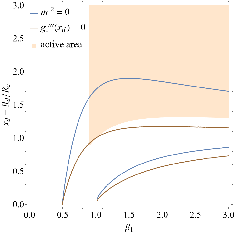
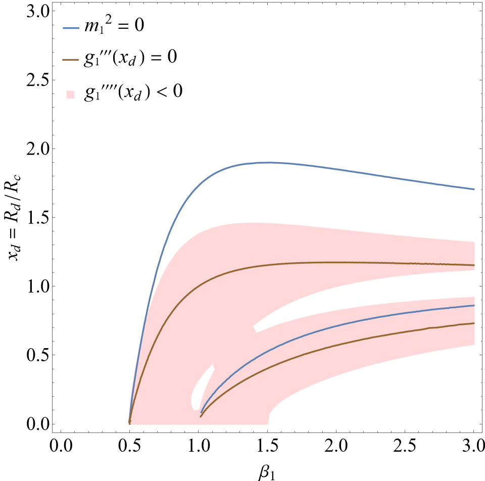
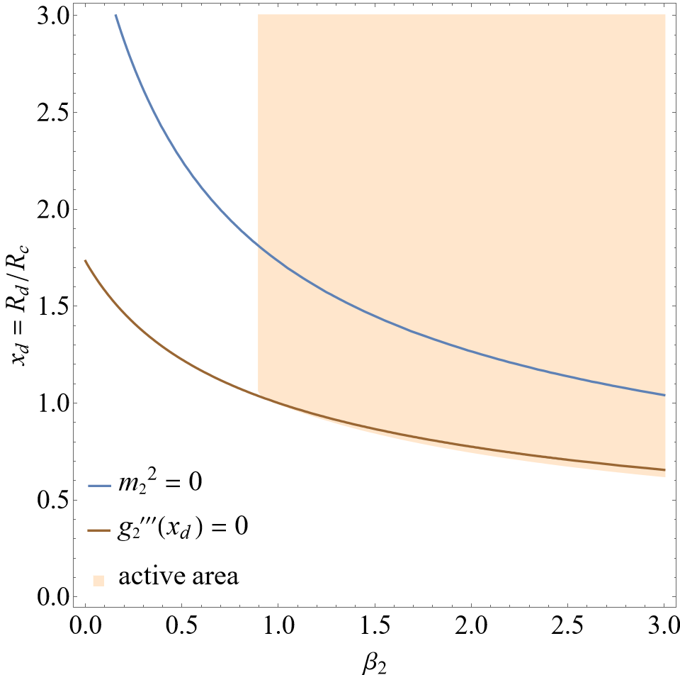
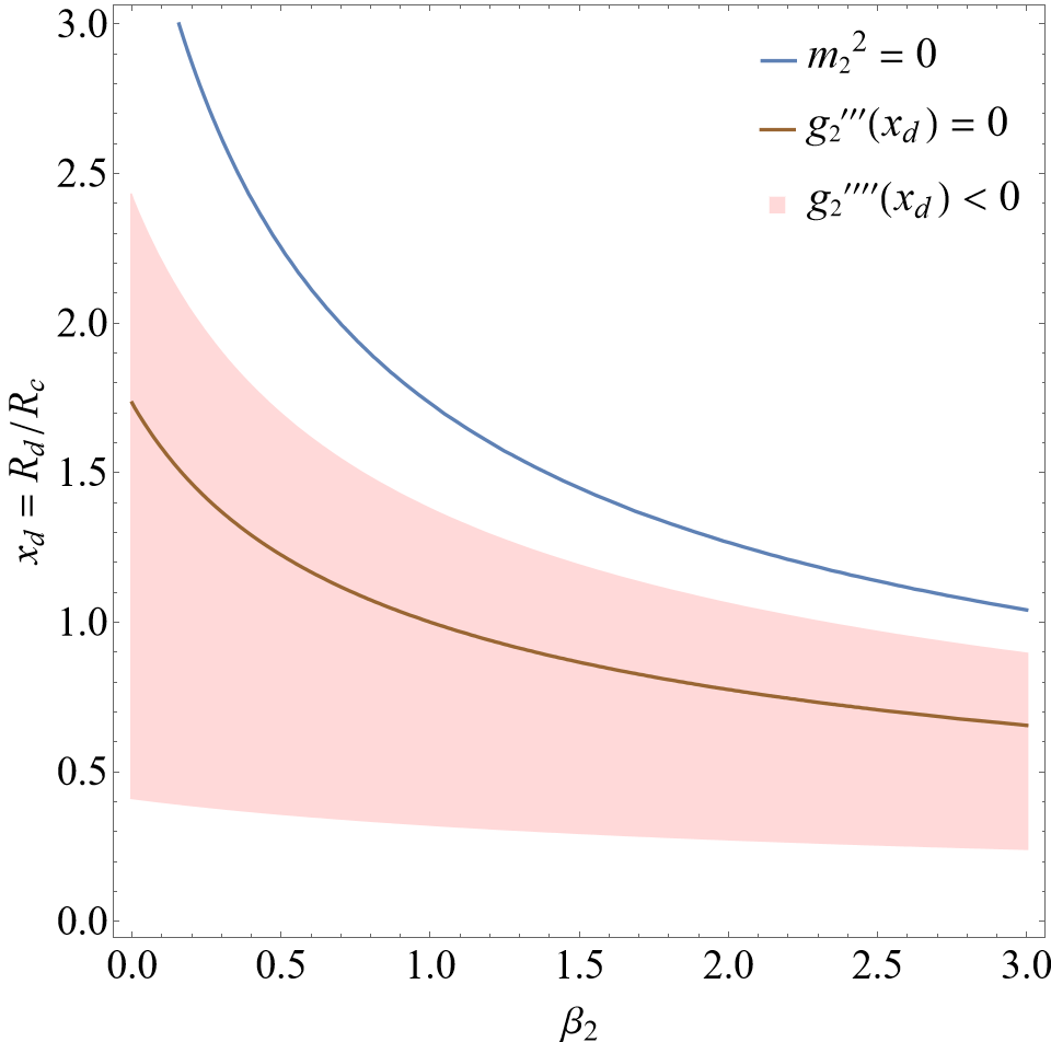
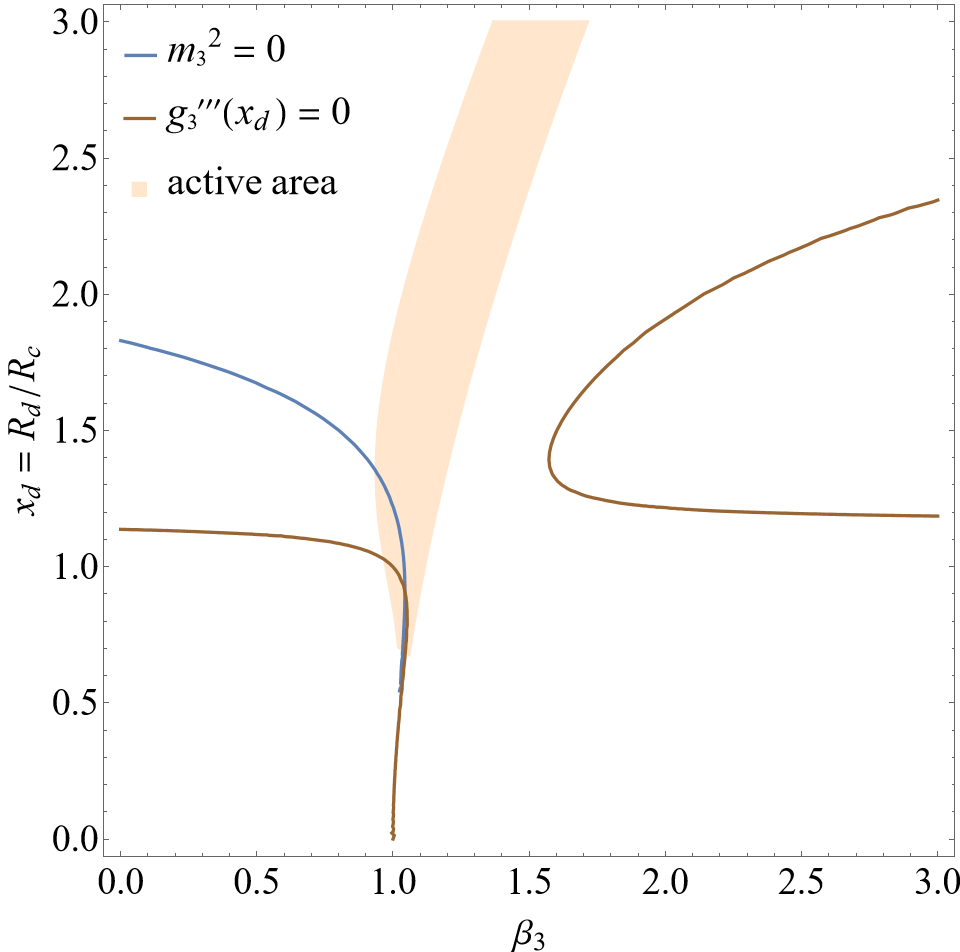
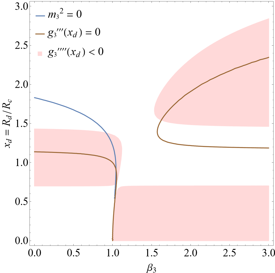
In this section, the constraints provided by section III are going to be taken into account in the specific models from Hu-Sawicki eq. (31), Starobinsky eq. (32) and Gogoi‑Dev eq. (33). The parameter spaces of and are applied, in which two viable areas are defined: one light orange area (active area) is described by the constraints from cosmology eqs. (40), (41), (42) and (43), while the other light red area is described by the constraint from effective potential eq. (64). Besides, two lines are defined: one blue solid line presents the solutions of , and the other brown solid line presents the solutions of . Only when the intersection of the two lines occurs in both the colored areas at the same time, will all the constraints be met, so that the de Sitter point of can become an active local minimum point to construct a stable massless scalar polarization.
IV.1 Active local minimum points
In figure 1, a possible intersection of and sits in the light red area, but it is definitely outside the light orange area. It implies that the constraints cannot be met concurrently, and hence the Hu-Sawicki model is inapplicable for a stable massless scalar polarization. In figure 2, it can be seen that the light orange area wraps and while the light red area wraps . Because there is no intersection between the two lines (even for ), the Starobinsky model is also inapplicable for a stable massless scalar polarization.
In figure 3, there is an intersection between and , and its coordinate is around (, ). By using eq. (46), one obtains , agreeing with the required range . Different from figure 1 and figure 2, the intersection occurs in both the light red and the light orange areas at the same time, which means that all constraint conditions can be met and an active local minimum point can be reached. Therefore, the Gogoi-Dev model is feasible for a stable massless scalar polarization.
The results indicate that the models of Hu-Sawicki and Starobinsky cannot be used to build up a stable massless scalar polarization, while Gogoi-Dev model can do that. Because these involved models have the same freedom degree, the reason for the difference should lie in the model structure rather than the number of free parameters. Obvious evidence can be seen in the active areas constructed by a series of inequalities. The active areas in figures 1, 2 and 3 visibly own different shapes, and these shapes are drawn by the derivatives and parameter bounds of . In the next subsection, we are going to examine the feasibility of Gogoi-Dev model in massless case in more detail.
IV.2 Satisfied constraint conditions
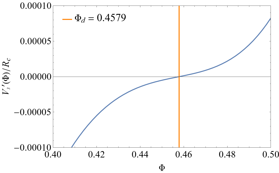
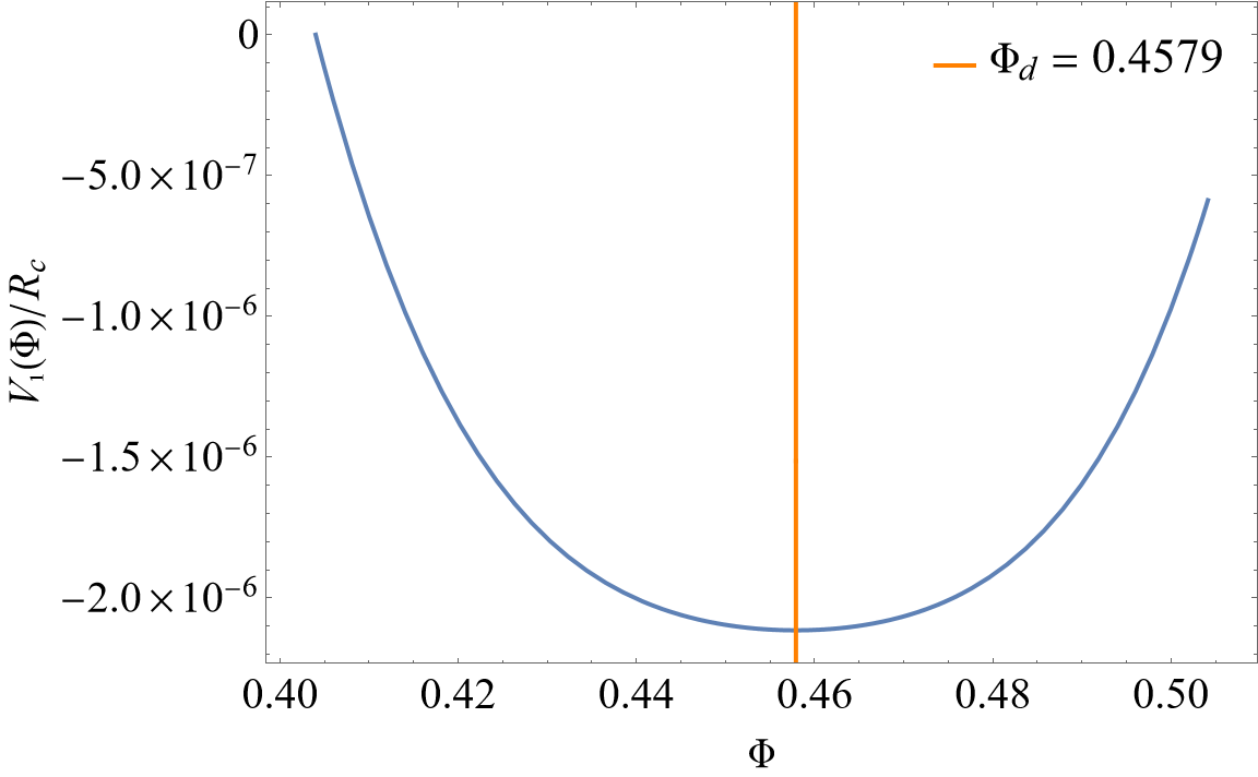
The constraint conditions eqs. (61), (62), (63) and (64) are aimed at giving a local minimum of the effective potential . In order to show this clearly, some figures will be drawn for Gogoi-Dev model to reflect how change with . To start with, based on the intersection coordinate given in subsection IV.1, the model parameters and are determined. After that, we apply eqs. (55), (56) and (57) to convert , and to the functions described by the parameter , so that the figures of parametric functions about and versus can be drawn with the change of . In figure 4, there is a zero value for at , and on the left-hand side of while on the right-hand side of . Thus, has a local minimum at , agreeing with the result of the picture of . Here is drawn by integrating from to () for avoiding the effect of extreme points.
Eqs. (40) and (41), the stability conditions for at , have been satisfied for Gogoi-Dev model. Therefore, eqs. (38) and (39), the stability conditions for in , should be checked in the following part. Because , both and need to be met in and . The range of will not be strictly defined, since its range depends on the different values of the model parameter . In other words, if there is a continuous range tightly attached to the left-hand side of , and and are met in this continuous range, we believe that these stability conditions could be satisfied in . In figure 5, we can see that in , so the stability condition eq. (39) is true for Gogoi-Dev model. On the other hand, there are in () and . Because can be regarded as with the adjustable parameter , the stability condition eq. (38) is also true for Gogoi-Dev model. To sum up, the stability in the curvature range is not violated for Gogoi-Dev model.
V Discussions and conclusions
The additional polarization of gravity is the scalar polarization, which is a mix of the longitudinal and the breathing modes. When the scalar mass given by eq. (5) vanishes, the massless scalar polarization will correspond to a pure breathing mode. However, in order to keep a settled perturbation of space-time, the constraints for effective potential eqs. (49) and (50) are used to make the scalar mass always positive, so that the massless scalar polarization seems to be excluded from . But we indicate that the constraints should be changed to more general forms eqs. (51) and (52), and the original constraints are just the special examples of eqs. (51) and (52) for . Under the more general constraints, the scalar mass are allowed to be zero, and the case of is studied in our paper.
In 3-parameter models eqs. (21), (22) and (23) which are regarded as viable dark energy models, we have analyzed the possibility of the existence of stable massless scalar polarizations. To get a stable massless scalar polarization in gravity, the constraints from two aspects need to be considered: one is the cosmology in subsection III.1, and the other one is the effective potential in subsection III.2. The results show that both Hu-Sawicki and Starobinsky models fail to build up a stable massless scalar polarization. On the contrary, Gogoi-Dev model can meet all kinds of constraints and lead to a stable massless scalar polarization. Therefore, the existence of stable massless scalar polarization in gravity should not be ignored. In other words, if a massless scalar polarization (or pure breathing mode) is observed, gravity should not be removed from these selectable modified gravity models.
The tested models all have 3 parameter degrees of freedom, but their abilities to maintain stable massless scalar polarizations are obviously different. It means that the model structure (or function expression) of gravity could influence the results of scalar polarization. That is to say, the scalar polarization is model-dependent for gravity. It is possible for us to distinguish various models by examining whether they have stable massless scalar polarizations. For those feasible models, when a massless scalar polarization is observed, some strict parameter constraints would be imposed on them. Under these constraints, every free parameter coming from 3-parameter models could only take a fixed value (here parameter will be determined if the de Sitter background curvature is fixed). For multi-parameter models, these constraints might be loosened, but they are still considerable to help us limit the ranges of free parameters. To sum up, the massless scalar polarization can be used to distinguish different models, and is expected to provide effective observation constraints on model parameters. We hope to study its role in other modified gravity theories in the future.
Acknowledgements.
We are grateful to Bao-Min Gu for helpful discussions. The work is in part supported by NSFC Grant No.12205104, “the Fundamental Research Funds for the Central Universities” with Grant No. 2023ZYGXZR079, the Guangzhou Science and Technology Project with Grant No. 2023A04J0651 and the startup funding of South China University of Technology.References
- [1] A.G. Riess, et al., Observational Evidence from Supernovae for an Accelerating Universe and a Cosmological Constant, The Astronomical Journal, 116 (1998) 1009.
- [2] M. Tegmark, et al., Cosmological parameters from SDSS and WMAP, Physical Review D, 69 (2004) 103501.
- [3] D.N. Spergel, et al., Three-Year Wilkinson Microwave Anisotropy Probe (WMAP) Observations: Implications for Cosmology, The Astrophysical Journal Supplement Series, 170 (2007) 377.
- [4] E.J. Copeland, M. Sami, S. Tsujikawa, DYNAMICS OF DARK ENERGY, International Journal of Modern Physics D, 15 (2006) 1753-1935.
- [5] T.P. Sotiriou, V. Faraoni, theories of gravity, Reviews of Modern Physics, 82 (2010) 451-497.
- [6] A. De Felice, S. Tsujikawa, f(R) Theories, Living Reviews in Relativity, 13 (2010) 3.
- [7] A. De Felice, S. Tsujikawa, Generalized Brans-Dicke theories, Journal of Cosmology and Astroparticle Physics, 2010 (2010) 024.
- [8] A. Avilez, C. Skordis, Cosmological Constraints on Brans-Dicke Theory, Physical Review Letters, 113 (2014) 011101.
- [9] R.V. Wagoner, Scalar-Tensor Theory and Gravitational Waves, Physical Review D, 1 (1970) 3209-3216.
- [10] M. Crisostomi, K. Koyama, G. Tasinato, Extended scalar-tensor theories of gravity, Journal of Cosmology and Astroparticle Physics, 2016 (2016) 044.
- [11] A.S. Sefiedgar, K. Atazadeh, H.R. Sepangi, Generalized virial theorem in Palatini gravity, Physical Review D, 80 (2009) 064010.
- [12] L.S. Collaboration, et al., Observation of Gravitational Waves from a Binary Black Hole Merger, Physical Review Letters, 116 (2016) 061102.
- [13] L.S. Collaboration, et al., GW170817: Observation of Gravitational Waves from a Binary Neutron Star Inspiral, Physical Review Letters, 119 (2017) 161101.
- [14] J. Luo, et al., TianQin: a space-borne gravitational wave detector, Classical and Quantum Gravity, 33 (2016) 035010.
- [15] G. Wang, W.-B. Han, Observing gravitational wave polarizations with the LISA-TAIJI network, Physical Review D, 103 (2021) 064021.
- [16] T. Liu, X. Lou, J. Ren, Pulsar Polarization Arrays, Physical Review Letters, 130 (2023) 121401.
- [17] D.M. Eardley, D.L. Lee, A.P. Lightman, Gravitational-Wave Observations as a Tool for Testing Relativistic Gravity, Physical Review D, 8 (1973) 3308-3321.
- [18] L.S.C. The, et al., Tests of general relativity with the binary black hole signals from the LIGO-Virgo catalog GWTC-1, Physical Review D, 100 (2019) 104036.
- [19] P.T.H. Pang, R.K.L. Lo, I.C.F. Wong, T.G.F. Li, C. Van Den Broeck, Generic searches for alternative gravitational wave polarizations with networks of interferometric detectors, Physical Review D, 101 (2020) 104055.
- [20] F.A.E. Pirani, Republication of: On the physical significance of the Riemann tensor, General Relativity and Gravitation, 41 (2009) 1215-1232.
- [21] D. Liang, Y. Gong, S. Hou, Y. Liu, Polarizations of gravitational waves in gravity, Physical Review D, 95 (2017) 104034.
- [22] M.E.S. Alves, O.D. Miranda, J.C.N. de Araujo, Probing the f(R) formalism through gravitational wave polarizations, Physics Letters B, 679 (2009) 401-406.
- [23] Y.-H. Hyun, Y. Kim, S. Lee, Exact amplitudes of six polarization modes for gravitational waves, Physical Review D, 99 (2019) 124002.
- [24] É.É. Flanagan, S.A. Hughes, The basics of gravitational wave theory, New Journal of Physics, 7 (2005) 204.
- [25] Y.-Q. Dong, Y.-Q. Liu, Y.-X. Liu, Polarization modes of gravitational waves in general modified gravity: General metric theory and general scalar-tensor theory, Physical Review D, 109 (2024) 044013.
- [26] M.E.S. Alves, Testing gravity with gauge-invariant polarization states of gravitational waves: Theory and pulsar timing sensitivity, Physical Review D, 109 (2024) 104054.
- [27] D.J. Gogoi, U. Dev Goswami, Gravitational waves in gravity power law model, Indian Journal of Physics, 96 (2022) 637-646.
- [28] S. Tsujikawa, Observational signatures of dark energy models that satisfy cosmological and local gravity constraints, Physical Review D, 77 (2008) 023507.
- [29] Y. Louis, L. Chung-Chi, G. Chao-Qiang, Gravitational waves in viable f(R) models, Journal of Cosmology and Astroparticle Physics, 2011 (2011) 029.
- [30] V. Müller, H.J. Schmidt, A.A. Starobinsky, The stability of the de Sitter space-time in fourth order gravity, Physics Letters B, 202 (1988) 198-200.
- [31] X. Zhang, J. Yu, T. Liu, W. Zhao, A. Wang, Testing Brans-Dicke gravity using the Einstein telescope, Physical Review D, 95 (2017) 124008.
- [32] T. Faulkner, M. Tegmark, E.F. Bunn, Y. Mao, Constraining gravity as a scalar-tensor theory, Physical Review D, 76 (2007) 063505.
- [33] J. Lu, Y. Wu, W. Yang, M. Liu, X. Zhao, The generalized Brans-Dicke theory and its cosmology, The European Physical Journal Plus, 134 (2019) 318.
- [34] D.J. Gogoi, U. Dev Goswami, A new f(R) gravity model and properties of gravitational waves in it, The European Physical Journal C, 80 (2020) 1101.
- [35] J.D. Barrow, A.C. Ottewill, The stability of general relativistic cosmological theory, Journal of Physics A: Mathematical and General, 16 (1983) 2757.
- [36] Y. Gong, S. Hou, The Polarizations of Gravitational Waves, in: Universe, 2018.
- [37] W. Hu, I. Sawicki, Models of cosmic acceleration that evade solar system tests, Physical Review D, 76 (2007) 064004.
- [38] A.A. Starobinsky, Disappearing cosmological constant in f(R) gravity, JETP Letters, 86 (2007) 157-163.
- [39] S.A. Appleby, R.A. Battye, A.A. Starobinsky, Curing singularities in cosmological evolution of F(R) gravity, Journal of Cosmology and Astroparticle Physics, 2010 (2010) 005.
- [40] H. Nariai, Gravitational Instability of Regular Model-Universes in a Modified Theory of General Relativity, Progress of Theoretical Physics, 49 (1973) 165-180.
- [41] V.T. Gurovich, A.A. Starobinskii, Quantum effects and regular cosmological models, Zh. Eksp. Teor. Fiz. (USSR), 77 (1979) 1683-1700.
- [42] A.D. Dolgov, M. Kawasaki, Can modified gravity explain accelerated cosmic expansion?, Physics Letters B, 573 (2003) 1-4.
- [43] S. Capozziello, S. Tsujikawa, Solar system and equivalence principle constraints on gravity by the chameleon approach, Physical Review D, 77 (2008) 107501.
- [44] S. Jana, S. Mohanty, Constraints on theories of gravity from GW170817, Physical Review D, 99 (2019) 044056.
- [45] S. Capozziello, A. Stabile, A. Troisi, Spherically symmetric solutions in f(R) gravity via the Noether symmetry approach, Classical and Quantum Gravity, 24 (2007) 2153.
- [46] M.M. Ivanov, A.V. Toporensky, STABLE SUPER-INFLATING COSMOLOGICAL SOLUTIONS IN f(R)-GRAVITY, International Journal of Modern Physics D, 21 (2012) 1250051.