STAR DISCREPANCY BOUNDS BASED ON HILBERT SPACE FILLING CURVE STRATIFIED SAMPLING AND ITS APPLICATIONS
Abstract.
In this paper, we consider the upper bound of the probabilistic star discrepancy based on Hilbert space filling curve sampling. This problem originates from the multivariate integral approximation, but the main result removes the strict conditions on the sampling number of the classical grid-based jittered sampling. The main content has three parts. First, we inherit the advantages of this new sampling and achieve a better upper bound of the random star discrepancy than the use of Monte Carlo sampling. In addition, the convergence order of the upper bound is improved from to . Second, a better uniform integral approximation error bound of the function in the weighted space is obtained. Third, other applications will be given. Such as the sampling theorem in Hilbert spaces and the improvement of the classical Koksma-Hlawka inequality. Finally, the idea can also be applied to the proof of the strong partition principle of the star discrepancy version.
Key words and phrases:
Star discrepancy; Stratified sampling; Hilbert space filling curve; Integral approximation.2020 Mathematics Subject Classification:
11K38, 65D30.1. Introduction
Many problems in industry, statistics, physics and finance need to introduce multivariable integrals. In order to effectively represent, analyze and process these integrals on the computer, it is necessary to discretize the sample points. A natural problem is whether these discrete sampling values can achieve the optimal fast convergence approximation of multivariable integrals. This is investigated by the discrepancy function method and sampling theory. And which also makes it a popular research topic in applied mathematics and engineering science.
For the multivariate function integral defined on a dimensional unit cube, if a discrete sampling point set is selected, it can be approximated by the sample mean . Then the approximation error can be calculated by:
Among various techniques to estimate the error of , star discrepancy has proven to be among the most efficient approaches. Star discrepancy was first used to measure the irregularity of the point distribution. For a point set , the star discrepancy is defined as follows:
| (1.1) |
where denotes the -dimensional Lebesgue measure, and denotes the characteristic function defined on the -dimensional rectangle .
A well-known result in discrepancy theory is the Koksma-Hlawka inequality [1, 2]. It shows that the integral approximation error of any multivariate function can be separated into two parts, one is the star discrepancy of the defined point set , and the other is the total variation of the function (under the definition of Hardy and Krause), i.e,:
| (1.2) |
The equation (1.2) indicates that when is a function of bounded variation, a smaller upper bound on the star discrepancy yields a more accurate approximation error of the integration. Therefore, we focus on the research of the star discrepancy in the following.
There are many kinds of constructive sampling sets, also known as low discrepancy point sets [3], which obtain a satisfactory convergence rate of star discrepancy bound. For a fixed dimension , it can reach , where is a constant that depends only on the dimension . This kind of point set is widely used in many fields, such as colored noise, learning theory and finance [4, 5, 6, 7], but this kind of point set also has some limitations. First of all, the convergence rate is strongly dependent on the dimensions. For high dimensional space, the convergence rate becomes slower, even worse than the convergence rate obtained by classical Monte Carlo in some cases. While the classical Monte Carlo sampling method is independent of the dimensions, so it has strong applicability for especially large-dimensional data. Secondly, because the low discrepancy point set is a constructive sampling, it is difficult to deal with a large number of point sets generated by random sampling in real life, such as the processing of noise-contaminated signals. Therefore, it is necessary to explore a new sampling method that inherits the fast convergence characteristics of low discrepancy point sets in moderate dimensions and the strong applicability of Monte Carlo point sets to high dimensions.
In order to achieve a better approximation effect for multivariate integrals in higher dimensions, a large number of points must be sampled if we use the low discrepancy point sets. Which loses information about the moderate sample size. In other words, if it is required to find the optimal upper bound of the star discrepancy in the higher dimensional space under the moderate sample size, the low discrepancy point set is not applicable. Therefore, in recent years, many scholars have carried out a series of studies on this problem and tried to use the appropriate sampling point set. This study is called the search for the optimal pre-asymptotic star discrepancy bound. In 2001, Heinrich, Novak [8] et al. proved that the optimal pre-asymptotic upper bound can be obtained as long as the number of sampling points linearly depends on the dimension, and the upper bound is , where is an unknown positive constant. In 2011, Aistleitner [9] calculated that is at most 10. This constant has been improved to 2.53 [10] so far. From a practical point of view, the following probabilistic pre-asymptotic upper bound [11] can be obtained, that is,
| (1.3) |
holds with probability at least for the Monte Carlo point set .
Combined with the K-H inequality, it is easy to achieve the optimal probability approximation of the bounded variation function on the dimensional unit cube. Especially for high-dimensional data, this approximation overcomes some disadvantages of the traditional deterministic low discrepancy point sets, and gives a good approximation with a moderate sample size.
| (1.4) |
holds with probability at least for the Monte Carlo point set .
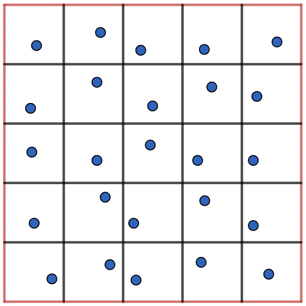
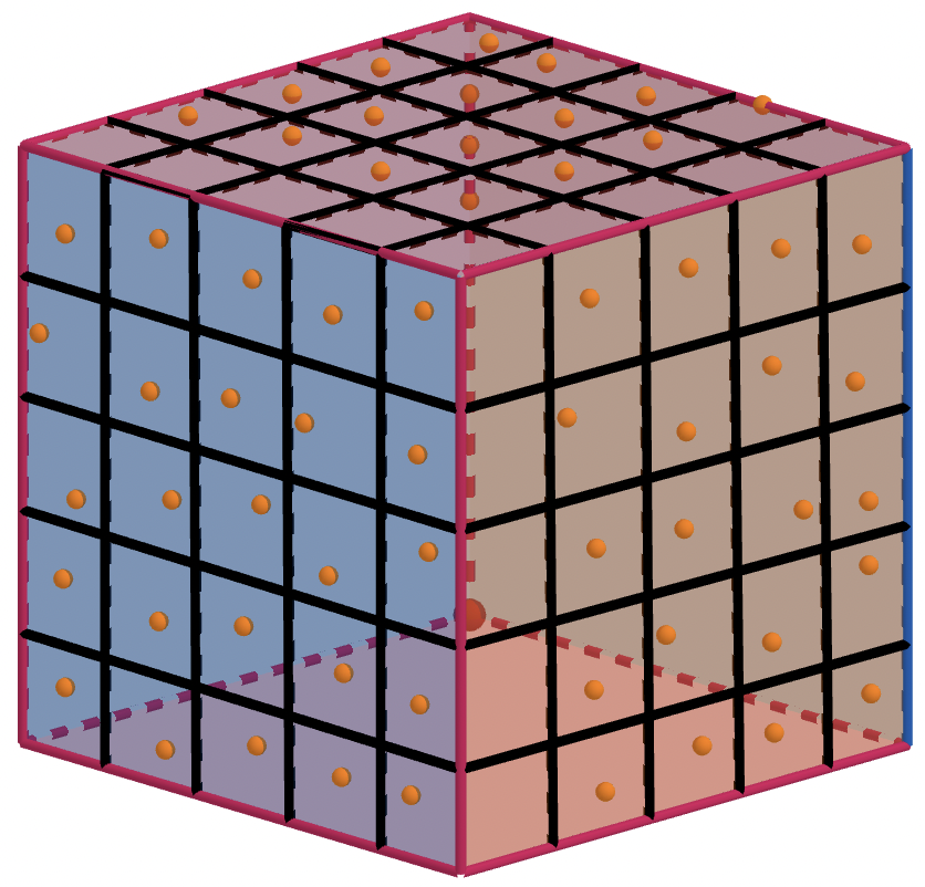
It is worth mentioning that the above pre-asymptotic star discrepancy bounds and the optimal probability approximation bounds are all obtained by using the Monte Carlo point set. Although the Monte Carlo method can get better approximation for high dimensional data, the convergence speed is slow, and the convergence speed is . How to improve this convergence speed and make the original approximation still applied to moderate sample size is a concern of scholars in recent years. Some scholars have noticed that the main reason for the slow convergence of the Monte Carlo method is the large variance of the sample mean function. Therefore, they have focused on the variance reduction technique and tried to use some new sampling methods to improve the approximation effect. For example, the probabilistic star discrepancy bound using Latin hypercube sampling [10] and the expected bound [12, 13] obtained by using jittered sampling. Jittered sampling is formed by isometric grid partition, and is divided into small sub-cubes each with side length Figures 1 and 2 give -dimensional and -dimensional illustrations.
Moreover, although the classical jittered sampling inherits some advantages of stratified sampling, it is more demanding for the number of sampling points, i.e., . The exponential dependence of the sampling number on , which will inevitably lead to the curse of dimensionality, so it is difficult to obtain the pre-asymptotic star discrepancy bound. However, jittered sampling retains the value of theoretical and numerical research, such as, it can achieve a faster convergence rate than the Monte Carlo sampling in a relatively low-dimensional space. While Latin hypercube sampling overcomes the dimensionality problem and reduces the variance of the sample mean, the star discrepancy convergence order is still , see [10].
If the problem is to reduce the error of the (1.2) under suitable sampling number, then for a class of bounded variation function spaces, there is
| (1.5) |
holds with probability at least .
So how to improve the convergence speed of the approximation error in (1.5) and preserve approximation information under the appropriate sampling number, based on the above introduction and discussion, there are two main ideas: one is to use the low discrepancy point sets, but note that the convergence order is , where is a constant that depends on the dimension . Generally for different point sets, is at least , so for high-dimensional space, the number of samples required is particularly large; the other is to use the idea of stratified sampling, but for classical jittered sampling, the disadvantage is that sampling points are required, and for high-dimensional space, it faces the curse of dimensionality. Therefore, it is necessary to return to the general stratified sampling method. We try to use a sampling method that combines the advantages of low discrepancy point sets and stratified sampling, and to overcome the dimension problem to a certain extent.
The Hilbert space filling curve sampling method coincidentally inherits many advantages of general stratified sampling, and we describe it in detail below. This method was developed by A. B. Owen, Z. He et al. to study the variance of the sample mean function [14, 15]. In our main result, we use Hilbert space filling curve sampling to obtain an improved upper bound of probability star discrepancy, and we give
| (1.6) |
holds with probability at least for the Hilbert space filling curve sampling set , where is an explicit and computable constant depending on and .
We can easily derive the probability star discrepancy bounds to the weighted form, and give the uniform probability approximation error in the weighted function space, that is, for a function in the weighted Sobolev space , the following
| (1.7) |
holds with probability at least for the Hilbert space filling curve sampling set .
The strong partition principle for the star discrepancy version is an open question mentioned in [12, 20], we use the probabilistic results to prove the following conclusion:
| (1.8) |
where is an arbitrary equivolume partition and is the corresponding stratified sampling set, and is simple random dimensional samples.
We also apply the main result to give explicit bounded expressions for a set of sampling inequalities in the general Hilbert space.
We prove:
holds with probability at least ( the probability that must hold), where , and belongs to Hilbert space.
In the end, we use the variant K-H inequality, combined with the obtained probabilistic star discrepancy bound, to give an approximation error for the piecewise smooth function defined on a Borel convex subset of .
We prove:
| (1.9) |
holds with probability at least , where is the star discrepancy of Hilbert space filling curve sampling and denotes the probability that the upper bound must hold. Besides,
| (1.10) |
The symbol is the partial derivative of with respect to those components of with index in .
2. Hilbert space filling curve sampling and some estimations
1. Hilbert space filling curve sampling
We first introduce Hilbert space filling curve sampling, which is abbreviated as HSFC sampling. We mainly adopt the definitions and symbols in [14, 15]. HSFC sampling is actually a stratified sampling formed by a special partition method.
Let be the first points of the van der Corput sequence(van der Corput 1935) in base . The integer is written in base as
| (2.1) |
for . Then, is defined by
| (2.2) |
The scrambled version of is written as
| (2.3) |
where are defined through random permutations of the . These permutations depend on for More precisely, and generally for
| (2.4) |
Each random permutation is uniformly distributed over the permutation of , and is mutually independent of the others. Thanks to the nice property of nested uniform scrambling, the data values in the scrambled sequence can be reordered such that
| (2.5) |
independently with
for .
Let
where is a mapping.
Then
is the corresponding stratified samples. Set be the diameter of , according to the property of HSFC sampling, the following estimation holds,
| (2.6) |
2. Minkowski content
We use the definition of Minkowski content in [16], which provides convenience for analysing the boundary properties of the test set in (1.1). For a set , define
| (2.7) |
where . If exists and is finite, then is said to admit dimensional Minkowski content. If is a convex set, then it is easy to see that admits dimensional Minkowski content. Furthermore, as the outer surface area of a convex set in is bounded by the surface area of the unit cube , which is .
3. -covers
To discretise the star discrepancy, we use the definition of covers as in[17].
Definition 2.1.
For any , a finite set of points in is called a –cover of , if for every , there exist such that and . The number denotes the smallest cardinality of a –cover of .
From [18], combined with Stirling’s formula, the following estimate holds for , that is, for any and ,
| (2.8) |
Furthermore, the following lemma provides a convenient way to estimate the star discrepancy with covers.
4. Bernstein inequality
At the end of this section, we will restate the Bernstein inequality which will be used in the estimation of star discrepancy bounds.
Lemma 2.3.
[19] Let be independent random variables with expected values and variances for . Assume (C is a constant) for each and set , then for any ,
3. Probabilistic star discrepancy bound for HSFC sampling
Theorem 3.1.
For integer number , and , then for the well defined dimensional stratified samples in Section 2, we have
| (3.1) |
holds with probability at least , where
Remark 3.2.
Theorem 3.1 improves the convergence order of the probabilistic star discrepancy bound. It is improved from to . Which can be compared to that of (1.3) and the part of the star discrepancy bound in (1.5). Secondly, the theorem is not as demanding as classical jittered sampling (i.e., it requires the number of sampling points to depend exponentially on the dimension, i.e., . In fact the number of sampling points in HSFC sampling method does not depend on the dimensions). Therefor, it gives a better integral approximation error in the pre-asymptotic case, which can be obtained by using the K-H inequality.
Proof.
Let be a subset of , then according to , it follows that
| (3.2) |
Now, for an arbitrary dimensional rectangle with diameter . When passes through the unit cube , we can choose two points such that and . Let and , then we have
and
| (3.3) |
We know that has a smaller diameter than , so we set it to , and has a larger diameter than , so we set it to . This forms a bracketing cover for the set , and from (2.8) and (3.3), we can derive the upper bound for the bracketing cover pair . It has a cardinality at most . Therefore, from the lemma 2.2, we obtain
| (3.4) |
For an anchored box in , it is easy to check that is representable as a disjoint union of entirely contained in and the union of pieces which are the intersections of some and , i.e,
| (3.5) |
where denote the index-sets.
By the definition of Minkowski content, for any , there exists such that whenever .
From (2.6), the diameter for each is at most . We can assume , then and ; thus
Without loss of generality, we can set , and combined with the fact that , it follows that
| (3.6) |
The same argument (3.6) applies to test sets and .
For or , set
| (3.7) |
is also a test rectangle, which can be divided into two parts
| (3.8) |
and the cardinality of is at most according to the estimate.
Let
| (3.9) |
If we define new random variables as follows
| (3.10) |
then from the above discussions, we have
| (3.11) | ||||
Since
| (3.12) |
hence
| (3.13) |
| (3.14) |
Let and , then we have
| (3.15) |
Therefore, from Lemma 2.3, for every , we have,
| (3.16) |
Let
| (3.17) |
Then using covering numbers, we have
| (3.18) |
Let , and we choose
| (3.19) |
By substituting into (3.18), we have
| (3.20) |
Combining above and (3.14), we obtain
| (3.21) | ||||
holds with probability at least .
Thus, obviously, we have
| (3.22) | ||||
holds with probability at least .
| (3.23) | ||||
where
| (3.24) |
The proof is completed. ∎
4. Applications of the main result
The following will give three applications of the theorem 3.1. One is the application of uniform integral approximation in weighted function space, and the other is to prove the strong partition principle of star discrepancy version. The strong partition principle is the problem proposed by [20, 21], which has been perfectly solved for the discrepancy, but remains to be solved for the star discrepancy version. The third is the sampling theorem in general Hilbert space. Finally, it is applied to the integral approximation problem on the Borel convex subset in .
4.1. Uniform integral approximation for functions in weighted function space
Many high-dimensional problems in practical applications have low effective dimension [22], that is, they have different weights for the function values of different components. Therefore, the problem is abstracted as finding the uniform integral approximation error in weighted Sobolev space.
Let be a Sobolev space, for functions , is differentiable for any variable and has a finite module for its first-order differential. For , the norm in is defined as
where and .
Then for weighted Sobolev space , its norm is
| (4.1) |
Considering the problem of function approximation in space. The sample mean method can still be used, for
and sample mean function
We consider the worst-case error
Then according to Hlawka and Zaremba identity [23], we have
For uniform integral approximation in weighted Sobolev spaces, we have the following theorem:
Theorem 4.1.
Let be functions in Sobolev sapce. Let integer , and . Let be some integers, be constants such that holds for all , and . Then for dimensional Hilbert space filling curve samples , we have
| (4.2) | ||||
holds with probability at least , where
Proof.
In theorem 3.1, we choose the probability . Which holds for some positive constant and for all , where is constant such that holds for all , and we choose
and .
Let
For a given number of sample points and dimension , we consider the following set
where . In addition, for , we define
Then we have
Hence,
According to and , for all and , we have and . Thus, , then
Based on this inequality, we obtain a formula that holds for all
Thus for every , we get
holds with probability at least .
The proof is completed. ∎
4.2. Strong partition principle for star discrepancy
For stratified sampling, [13] proves that the classical jittered sampling can obtain a better expected star discrepancy bound than the traditional Monte Carlo sampling. Which means that the jittered sampling is the optimization of Monte Carlo sampling when the number of sampling points is . Then the problem is how to directly compare the size of the expected star discrepancy under different sampling methods, rather than the optimization of the bound. It refers to how to prove the partition principle of star discrepancy. That is, the expected star discrepancy of the HSFC stratified sampling( here is no longer limited to the jittered case) must be smaller than the expected star discrepancy of simple random sampling.
Theorem 4.2.
For integers , and . For well-defined Hilbert space filling curve samples , and simple random dimensional samples , then
| (4.3) |
Proof.
For arbitrary test set , we unify a label . Which is the sampling point sets formed by different sampling models, and we consider the following discrepancy function,
| (4.4) |
For an equivolume partition , we divide the test set into two parts, one being the disjoint union of completely contained by , and the other being the union of the remaining parts which are the intersections of some and , i.e.,
| (4.5) |
where are two index sets.
We set
Furthermore, for the equivolume partition of and the corresponding stratified sampling set , we have
| (4.6) | ||||
For sampling sets and , we have
| (4.7) |
and
| (4.8) |
Hence, we have
| (4.9) |
Now we exclude the case of equality in (4.9), which means that the following formula holds,
| (4.10) |
for and for almost all .
Hence,
| (4.11) |
for almost all and all , which implies . This is not impossible for
For set , we have
| (4.12) |
The same analysis for the set as , we have
| (4.13) |
For the test set , we choose and such that and , then (,) form the covers. For and , we can divide them into two parts as we did for (4.5). Let
and
We have the same result for and . To unify the two cases and (because and are generated from two test sets with the same cardinality, and the cardinality is the covering numbers), we consider a set which can be divided into two parts
| (4.14) |
where are two index sets. In addition, we set the cardinality of to be at most (the covering numbers, where we choose ), and we let
We define new random variables , as follows
Then,
| (4.15) | ||||
Since
we get
| (4.16) |
| (4.17) |
Let
Therefore, from Lemma 2.3, for every , we have,
Let then using cover numbers, we have
| (4.18) |
Combining with (4.17), we get
| (4.19) | ||||
For point sets and , if we let
Then (4.13) implies
Besides, as (4.19), we have
| (4.20) | ||||
and
Suppose , and we substitute
into (4.20), then we have
| (4.21) |
Therefore, from (4.21), it can be easily verified that
| (4.22) |
holds with probability at least .
Combined with covering numbers(where ), we get,
| (4.23) | ||||
holds with probability at least . The last inequality in (4.23) holds because holds for all .
Same analysis with point set , we have
| (4.24) | ||||
holds with probability at least .
Now we fix a probability value in (4.23), i.e. we assume that (4.23) holds with probability exactly , where . If we choose this in (4.24), we have
holds with probability
Therefore from , we obtain,
| (4.25) |
holds with probability where .
We use the following fact to estimate the expected star discrepancy
| (4.26) |
where denotes the star discrepancy of point set .
By substituting into (4.23), we obtain
| (4.27) |
holds with probability . Then (4.27) is equivalent to
Now releasing and let
| (4.28) |
| (4.29) |
and
| (4.30) |
Then
| (4.31) |
Thus from (4.26) and , we have
| (4.32) | ||||
Furthermore, from (4.25), we have
From we obtain
Hence,
| (4.33) |
∎
Corollary 4.3.
For any equivolume partitions and the corresponding stratified sampling set . For simple random dimensional samples , we have
| (4.34) |
Proof.
For and , it follows that
| (4.35) | ||||
For simple random sampling set , we have
| (4.36) |
According to the proof process of Theorem 4.2, we have
| (4.37) |
and the desired result. ∎
Remark 4.4.
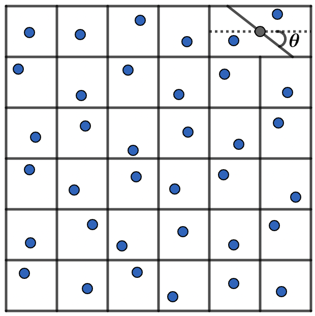
An example: For a grid-based equivolume partition in two dimensions, the two squares in the upper right corner are merged to form a rectangle
where are three positive constants.
For the merged rectangle , we use a series of straight-line partitions to divide the rectangle into two equal-volume parts, which will be converted to a one-parameter model if we set the angle between the dividing line and the horizontal line across the center , where we suppose that . From simple calculations, we can conclude that the arbitrary straight line must pass through the center of the rectangle. For convenience of notation, we set this partition model in the two-dimensional case, see Figure 3.
Now, we consider the dimensional cuboid
| (4.38) |
and its partitions into two closed, convex bodies with
| (4.39) |
We choose in , which is denoted by , and obtain
| (4.40) |
Then, we have the following result.
Corollary 4.5.
For any . For the class of equivolume partitions and the corresponding stratified sampling set . For simple random samples , we have
| (4.41) |
4.3. Sampling theorem in Hilbert space
The sampling problem attempts to reconstruct or approximate a function from its sampled values on the sampling set [24]. To solve this problem, it is necessary to specify the function space, since the theoretical and numerical analysis may differ for different function spaces. Common sampling function spaces are: (i)band-limited signals [25]; (ii)signals in some shift-invariant spaces [34, 32, 33, 26, 30, 31]; (iii)non-uniform splines [28, 29]; (iv)sum of some of the above signals [27], and so on.
Well-posedness of the sampling problem implies that the following inequalities must hold:
| (4.42) |
where and are some positive constants. The inequalities (4.42) indicate that a small change in a sampled value causes only a small change in . This implies that the sampling is stable, or equivalently, that the reconstruction of from its samples is continuous. Due to the randomness in the choice of the sampling points, our goal is to choose the following probability estimate:
| (4.43) |
where can be taken as arbitrarily small.
In this subsection, we study the problem of stratified sampling sets, and give explicit bounded expressions for a set of sampling inequalities in general Hilbert spaces.
Theorem 4.6.
For integers , and . Then for well-defined dimensional Hilbert space filling curve samples , we have
holds with probability at least , where , belongs to Hilbert space.
Proof.
Consider the following kernel function,
It is not realistic to measure exactly for samples , see discussions in [34]. A better assumption is that the sampling number has the following form:
| (4.44) |
where belongs to Hilbert space. For samples is a set of functionals acting on the function to produce the data . The functionals can reflect the characteristics of the sampling devices.
Therefore, we have
| (4.45) | ||||
and
| (4.46) | ||||
Therefore, according to (4.44), we obtain where .
∎
4.4. Application on Koksma–Hlawka inequality
The classical K-H inequality is not suitable for functions with simple discontinuities. While [35] proposes a variant K-H type inequality that is suitable for piecewise smooth functions of , where is smooth and is a Borel convex subset of . In this subsection, we will use the star discrepancy upper bound of Hilbert space filling curve sampling to give an approximation error in the piecewise smooth function space. First of all, there is the following lemma:
Lemma 4.7.
[35] Let be a piecewise smooth function on , and be a Borel subset of . Then for in , we have
| (4.48) |
where
| (4.49) |
and
| (4.50) |
The symbol is the partial derivative of with respect to those components of with index in , and the supremum is taken over all axis-parallel boxes .
Theorem 4.8.
For integers , and . Let be a piecewise smooth function on , and be a Borel convex subset of . Then for well-defined dimensional Hilbert space filling curve samples , we have
| (4.51) |
where was obtained in Theorem 3.1.
Where
| (4.52) |
The symbol is the partial derivative of with respect to those components of with index in .
Proof.
Because is a convex set, and in (4.49), is a convex set, so the test set is a convex set and . In addition, for the set and , and which satisfy , then and constitute cover. Through , we can obtain the cover number. Furthermore, according to the idea of the proof of theorem 3.1, we get the desired result. ∎
An example: For , let be the simplex
Define
Then one can show that
By theorem 4.8, for Hilbert space filling curve samples , and all convex sets contained in , we have
| (4.53) |
5. Conclusions
The convergence of the star discrepancy bound for HSFC-based sampling is , which matches the rate using jittered sampling sets and improves the rate using the classical MC method. The strict condition for the sampling number in the jittered case is removed, and the applicability of the new stratified sampling method for higher dimensions is improved. Although a faster convergence of the upper bound leads to a faster integration approximation rate, the strict comparison of the size of random star discrepancy under different stratified sampling models remains unresolved.
References
- [1] E. Hlawka, Funktionen von beschränkter variatiou in der theorie der gleichverteilung, Annali di Matematica Pura ed Applicata, 54(1961), 325-333.
- [2] JF. Koksma, Een algemeene stelling uit de theorie der gelijkmatige verdeeling modulo 1, Mathematica B (Zutphen), 11(1942/1943), 7-11.
- [3] J. Dick and F. Pillichshammer, Digital nets and sequences: Discrepancy theory and quasi-Monte Carlo integration, Cambridge University Press, 2010.
- [4] A. G. M. Ahmed, H. Perrier and D. Coeurjolly, et al, Low-discrepancy blue noise sampling, ACM Trans. Graph., 35(6)(2016), 1-13.
- [5] C. Cervellera and M. Muselli, Deterministic design for neural network learning: An approach based on discrepancy, IEEE Trans. Neural Netw., 15(3)(2004), 533-544.
- [6] Y. Lai, Monte Carlo and Quasi-Monte carlo methods and their applications, Ph.D. Dissertation, Department of Mathematics, Claremont Graduate University, California, USA, 1998.
- [7] Y. Lai, Intermediate rank lattice rules and applications to finance, Appl. Numer. Math., 59(2009), 1-20.
- [8] S. Heinrich, E. Novak, G. W. Wasilkowski and H. Woźniakowski, The inverse of the star-discrepancy depends linearly on the dimension, Acta Arith., 96(3)(2001), 279-302.
- [9] C. Aistleitner, Covering numbers, dyadic chaining and discrepancy, J. Complexity, 27(6)(2011), 531-540.
- [10] M. Gnewuch, N. Hebbinghaus, Discrepancy bounds for a class of negatively dependent random points including Latin hypercube samples, Ann. Appl. Probab., 31(4)(2021), 1944-1965.
- [11] C. Aistleitner and M. Hofer, Probabilistic discrepancy bound for Monte Carlo point sets, Math. Comp., 83(2014), 1373-1381.
- [12] F. Pausinger and S. Steinerberger, On the discrepancy of jittered sampling, J. Complexity, 33(2016), 199-216.
- [13] B. Doerr, A sharp discrepancy bound for jittered sampling, Math. Comp., 91(2022), 1871-1892.
- [14] Z. He, A. B. Owen, Extensible grids: uniform sampling on a space filling curve, J. R. Stat. Soc. Ser. B, 78(2016), 917-931.
- [15] Z. He, L. Zhu, Asymptotic normality of extensible grid sampling, Stat. Comput., 29(2019), 53-65.
- [16] L. Ambrosio, A. Colesanti, and E. Villa, Outer Minkowski content for some classes of closed sets, Math. Ann., 342(4)(2008), 727–748.
- [17] B. Doerr, M. Gnewuch, A. Srivastav, Bounds and constructions for the star-discrepancy via covers, J. Complexity, 21(2005), 691-709.
- [18] M. Gnewuch, Bracketing numbers for axis-parallel boxes and applications to geometric discrepancy, J. Complexity, 24(2)(2008), 154-172.
- [19] F. Cucker and D. X. Zhou, Learning theory: an approximation theory viewpoint, Cambridge University Press., 2007.
- [20] M. Kiderlen and F. Pausinger, On a partition with a lower expected -discrepancy than classical jittered sampling, J. Complexity 70(2022), https://doi.org/10.1016/j.jco.2021.101616.
- [21] M. Kiderlen and F. Pausinger, Discrepancy of stratified samples from partitions of the unit cube, Monatsh. Math., 195(2021), 267-306.
- [22] F. Y. Kuo and I. H. Sloan, Lifting the curse of dimensionality, Notices of the American Mathematical Society, 52(11)(2005), 1320–1328.
- [23] E. Novak and H. Woźniakowski, Tractability of Multivariate Problems, Volume II: Standard Information for Functionals, European Mathematical Society, 2010.
- [24] R. F. Bass and K. Gröchenig, Random sampling of bandlimited functions, Israel J. Math., 177(2010), 1-28.
- [25] R. F. Bass and K. Gröchenig, Relevant sampling of band-limited functions, Illinois J. Math., 57(2013), 43-58.
- [26] K. Gröchenig and H. Schwab, Fast local reconstruction methods for nonuniform sampling in shift-invariant spaces, SIAM J. Matrix Anal. Appl., 24(2003), 899-913.
- [27] Q. Y. Sun, Frames in spaces with finite rate of innovation, Adv. Comput. Math., 28(2008), 301-329.
- [28] W. C. Sun, Local sampling theorems for spaces generated by splines with arbitrary knots, Math. Comput., 78(2009), 225-239.
- [29] W. C. Sun and X. W. Zhou, Characterization of local sampling sequences for spline subspaces, Adv. Comput. Math., 30(2009), 153-175.
- [30] J. Xian and S. Li, Sampling set conditions in weighted finitely generated shift-invariant spaces and their applications, Appl. Comput. Harmon. Anal., 23(2007), 171-180.
- [31] J. B. Yang, Random sampling and reconstruction in multiply generated shift-invariant spaces, Anal. Appl., 17(2019), 323-347.
- [32] H. Fhr and J. Xian, Quantifying invariance properties of shift-invariant spaces, Appl. Comput. Harmon. Anal., 36(2014), 514-521.
- [33] H. Fhr and J. Xian, Relevant sampling in finitely generated shift-invariant spaces, J. Approx. Theory, 240(2019), 1-15.
- [34] A. Aldroubi and K. Gröchenig, Nonuniform sampling and reconstruction in shift-invariant spaces, SIAM Rev., 43(2001), 585-620.
- [35] G. Gigante, L. Brandolini, L. Colzani and G. Travaglini, On the koksma–hlawka inequality, J. Complexity, 29(2)(2013), 158–172.