Star graphs induce tetrad correlations:
for Gaussian as well as for binary variables
Abstract
Tetrad correlations were obtained historically for Gaussian distributions when tasks are designed to measure an ability or attitude so that a single unobserved variable may generate the observed, linearly increasing dependences among the tasks. We connect such generating processes to a particular type of directed graph, the star graph, and to the notion of traceable regressions. Tetrad correlation conditions for the existence of a single latent variable are derived. These are needed for positive dependences not only in joint Gaussian but also in joint binary distributions. Three applications with binary items are given.
keywords:
[class=AMS]keywords:
T1The work (also on ArXiv 1307.5396) reported in this paper was undertaken during the first author’s tenure of a Senior Visiting Scientist Award by the International Agency of Research on Cancer, Lyon.
, and
1 Introduction
Since the seminal work by Bartlett (1935) and Birch (1963), viewed in a larger perspective by Cox (1972), correlation coefficients were barely used as measures of dependence for categorical data. Instead, functions of the odds-ratio emerged as the relevant parameters in log-linear probability models for joint distributions and in logistic models, that is for regressions with a binary response. Compared with other possible measures of dependence, the outstanding advantage of functions of the odds-ratio is their variation independence of the marginal counts: odds-ratios are unchanged under different types of sampling schemes that result by fixing either the total number, , of observed individuals or the counts at the levels of one of the variables; see Edwards (1963).
As one consequence of the importance of odds-ratios for discrete random variables, it is no longer widely known that Pearson’s simple, observed correlation coefficient, say, coincides in contingency tables with the so-called Phi-coefficient, so that is, asymptotically and under independence of the two binary variables, a realization of a standard Gaussian distribution. As we shall see, some properties of correlation coefficients for binary variables, make them important for data generating processes that incorporate many conditional independences.
In particular, we look here at directed star graphs such as the one shown in Figure 1(a). Such graphs have one inner node, , from which arrows start and point to the uncoupled, outer nodes . To simplify notation, the inner node denotes also the corresponding random variable and both, the node and the variable, are called root. The random variables corresponding to the outer nodes, also called the leaves of the graph, are identified just by their index taken from .
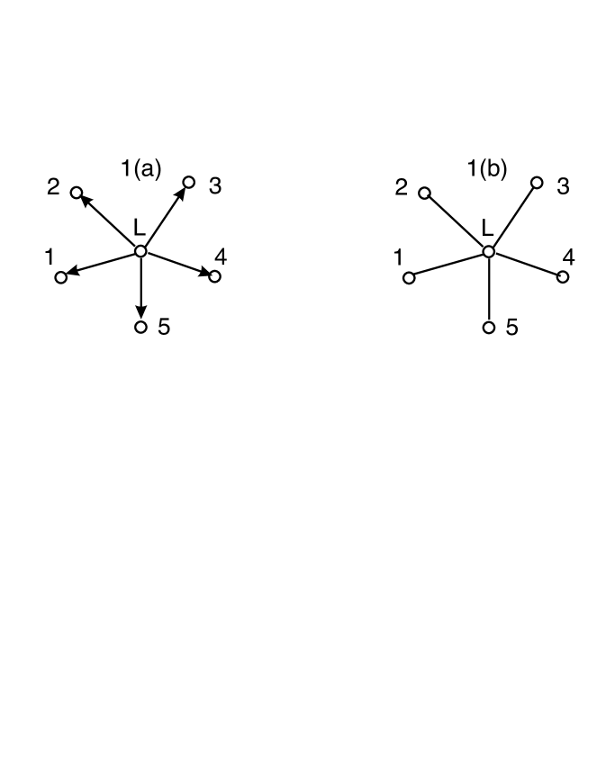
The independence structure of the directed star graph is mutual independence of the leaves given the root. In the condensed node notation, this is written as
| (1) |
In general, the types of variables can be of any kind. Densities, , that are said to be generated over the directed star graph with node set , may also be of any kind, provided that they have the above independence structure.
Each generated density is defined by conditional densities, , that are called regressions, and a marginal density, , of the root. In the condensed node notation, a joint density with the independence structure of a directed star graph, factorizes as
| (2) |
Directed star graphs belong to the class of regression graphs and to their subclass of directed acyclic graphs. Distributions generated over regression graphs have been named and studied as sequences of regressions and one knows when two regression graphs capture the same independence structure, that is when they are Markov equivalent, even though defined differently; see Theorem 1 in Wermuth and Sadeghi (2012). In particular, each directed star graph is Markov equivalent to an undirected star graph with the same node and edge set, such as in Figure 1(b), since it does not contain a collision V: , that is two uncoupled arrows meeting head-on.
Sequences of regressions are traceable if one can use the graph alone to trace pathways of dependence, that is to decide when a non-vanishing dependence is induced for an uncoupled node pair. For this, each edge present in the regression graph corresponds to a non-vanishing, conditional dependence that is considered to be strong in a given substantive context. In evolutionary biology, the required changes in dependences that are strong enough to lead to mutations, were for instance called ‘drastic’ by Neyman (1971). In general, special properties of the generated distributions are required in addition; see Wermuth (2012).
In the last century, regression graphs were not yet defined and properties of traceable regression unknown. Then, distributions generated over directed star graphs, in which the root corresponds to a variable that is never directly observed, have been studied separately under different distributional assumptions and with changing main objectives. Many of them were named item response models. In these contexts, the unobserved root is also called latent or hidden, the items are the observed variables.
For instance, Spearman (1904) suggested to measure general intelligence with similar quantitative tasks, a method now called factor analysis with a single latent variable. For confirmatory factor analyses, typically, a Gaussian distribution is assumed, after the observed variables are standardized to have mean zero and unit variance. Heywood (1931) and Anderson and Rubin (1956) derived necessary and sufficient conditions for the existence of one or more latent variables, without the constraint of non-vanishing, positive dependences of each item on the latent variables. The latter assumption arises however naturally when the items are to measure a specific latent ability or attitude or when they are the symptoms of a given disease.
For instance, when psychologists try to measure for children in a given age range, what is called the working memory capacity, then each item is the successful repetition – in reverse order – of a sequence of numbers. Typical tasks of the same difficulty are the sequences (3, 5, 7) and (2, 4, 6). The item difficulty increases, for instance, by presenting more numbers or numbers of two digits. For children with a higher capacity of the working memory, one expects more successes for tasks of the same difficulty as well as for tasks of increasing difficulty.
When instead, the leaves and the root of the star graph are both categorical, the resulting model is a latent class model, as proposed by Lazarsfeld (1950), again with an extensive follow-up literature. An important warning was given by Holland and Rosenbaum (1986): such a model can never be falsified when the number of levels of the latent variable is large compared to the number of cells in the observed contingency table. Expressed in other words, merely requiring conditional independence of categorical items given the latent variable imposes then no constraints on the observed distributions.
A general, testable constraint suggested by Holland and Rosenbaum (1986), that is now widely adopted in nonparametric item response theory, is to have a monotonically non-decreasing association of each item on ; see van der Ark (2012) or Mair and Hatzinger (2007). However, the underlying notion of ‘conditional association’, that had been proposed in probability theory, includes conditionally independent variables as being ‘conditionally associated’; see Esary, Proschan and Walkup (1967). By contrast, when one uses traceable regressions, each edge present in a graph excludes explicitly a corresponding conditional independence statement.
In this paper, we study similarities of joint Gaussian and of binary distributions generated over directed star graphs where all dependences of leaves, , on the root, , are positive and the root is unobserved but does not coincide with any leaf or with any combination of the leaves. In Section 2, we summarize results for star graphs and for their traceable regressions. In Section 3, we describe joint Gaussian distributions, so generated, and in Section 4, we study joint binary distributions, especially correlation constraints on the distribution of the leaves. Section 5, gives applications to binary distributions, Section 6 a general discussion. The Appendix contains a technical proof.
2 Marginalizing over the root in star graphs
A regression graph is said to be edge-minimal when each of its edges, that is present in the graph, indicates a non-vanishing dependence.
Definition 1.
Traceable regressions are generated over an edge-minmal, directed star graph, if (a) the density factorizes as in equation (2) and (b) is dependence-inducing by marginalizing over the root , that is yields for each pair of leaves a bivariate dependence, denoted by .
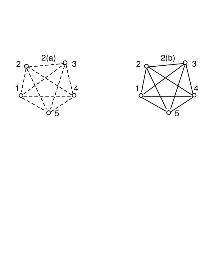
Thus, for traceable regressions with exclusively strong dependences, , in the generating star graph, each -edge in the induced complete covariance graph of the leaves, drawn as in Figure 2(a), indicates a non-vanishing dependence, . Probability distributions that do not induce such a dependence violate singleton-transitivity; see Table 1 in Wermuth (2012) for an example of such a family of distributions.
More consequences can be deduced, using strong dependences and the Markov equivalence of the directed to the undirected star graph with the same node and edge set, as in Figures 1(a) and 1(b). For a traceable distribution with an undirected star graph, such as in Figure 1(b), each edge in the induced complete concentration graph, obtained by marginalising over the root and drawn as in Figure 2(b), indicates a non-vanishing conditional dependence of each pair of leaves given the remaining leaves, denoted by .
In exponential family distributions, a covariance graph corresponds to bivariate central moments, a concentration graph to joint canonical parameters and a directed star graph to regression parameters. If Markov equivalent models are also parameter equivalent, then their parameter sets are in a one-to-one relation. This property does not hold in general, but for instance in joint Gaussian distribution, and in joint binary distributions that are quadratic exponential. More generally, Markov equivalence and parameter equivalence coincide when only a single parameter determines for each variable pair whether the pair is conditionally dependent or independent.
For traceability of a given sequence of regressions, the generated family of distributions needs to have three properties of joint Gaussian distributions, that are not common to all probability distributions. In addition to the dependence-inducing property (singleton-transitivity) stated in Definition 1, these are the intersection (downward combination) and the composition property (upward combination of independences); see Lněnička and Matúš (2007) equations (9) to (10) and Wermuth (2012) section 2.4.
Pairwise independences are said to combine downwards and upwards if
respectively, for any subset of the remaining nodes, of . Both of these properties are already needed if one is using graphs of mixed edges just to decide on implied independences; see Sadeghi and Lauritzen (2014).
In the context of directed star graphs, these two properties are a consequence of the special type of generating process. After removing any two arrows for , a directed star graph in arrows remains. Thus, by introducing two additional pairwise independences in a directed star graph, these independence statement combine downwards. The Markov equivalence of the directed to the undirected star graph implies that for any two nodes, the statement can be modified to with so that pairwise independences combine upwards.
3 Gaussian distributions generated over directed star graphs
In Gaussian distributions, each dependence is by definition linear and proportional to some (partial) correlation coefficient. Furthermore, there are no higher than two-factor interactions. In a traceable Gaussian distribution generated over a directed star graph, each directed edge indicates a simple, strong correlation, , called the loading of item on . Then for each item pair a simple correlation, is induced via
| (3) |
where denotes the partial correlation coefficient
In factor analysis, the latent root is assumed, without loss of generality, to have mean zero and unit variance. Typically, when the observed variances of the items are nearly equal, the items are transformed to have mean zero and unit variance, so that their correlation matrix is analyzed.
In general, the model parameters are known to be identifiable for ; see for instance Stanghellini (1997). For items, the positive loadings can be completely recovered using equations (3) for the positive, partial correlations of each leaf pair. The maximum-likelihood equations (Lawley, 1967) reduce to the same type of three equations so that a unique, closed form solution can be obtained, provided it exists, and be written as with
| (4) |
Clearly, these equations require for permissible estimates: . In that case, there can be no zero and no negative marginal or partial item correlation that cannot be removed by recoding some items. We give in Table 1 three examples of invertible correlation matrices, showing marginal correlations in the lower half and partial correlations in the upper half. The first two examples have no permissible solution for and illustrate so-called Heywood cases.
In the example on the left, . By equation (4), the estimated loading of item 1 is then equal to one, i.e. , so that item 1 cannot be distinguished from the latent variable itself. For the example in the middle, is larger than one, hence leads to an infeasible solution for a correlation coefficient. Thus even for a positive, invertible item correlation matrix, there may not exist a generating process via positive loadings on a single latent variable. The example on the right, has a perfect fit for the vector of estimated positive loadings in equation (4) as .
For items, proper positive loadings in equation (3), that is for all items , lead directly to a positive correlation matrix of the items, denoted in this paper by , that is to exclusively positive correlations, for in , and to a tetrad structure. Vanishing tetrads were defined by Spearman and coauthors and nowadays a popular search algorithm for models with possibly several latent variables is named Tetrad. This algorithm is based on and extends work by Spirtes, Glymour and Scheines (1993, 2001).
Definition 2.
A positive tetrad correlation matrix has dimension and elements such that for all item pairs and
| (5) |
Thus for any pair , the ratio of its correlations to variables in row of is the same as to variables in row , or, equivalently, there are vanishing tetrads: . Let denote a row vector of proper positive loadings, a diagonal matrix of elements , and a row vector of elements , where , then, as proven in the Appendix, the correlation matrix of the leaves and its inverse, the concentration matrix , are
| (6) |
Some important direct consequences of (6) are given next. Lemma 1 uses the notion of M(inkowski)-matrices that were named and studied by Ostrowski (1937, 1956) and discussed in connection to totally positive Gaussian distributions much later using the name MTP2 distributions; see e.g. Karlin and Rinott (1983). General MTP2 distributions are characterized by having no variable pair negatively associated given all remaining variables. We will use a more strict form of MTP2 that also excludes any variable pair being conditionally independent given all remaining variables.
Definition 3.
A square, invertible matrix is a complete M-matrix if all its diagonal elements are positive and all its off-diagonal elements are negative.
Lemma 1.
A positive tetrad correlation matrix, , generated over a star graph with proper positive loadings, , is invertible and is a symmetric, complete M-matrix with vanishing tetrads.
When we denote the elements of by , then by Lemma 1 and Definition 3, all the precisions, are positive and all concentrations are negative, that is , for all , if is a complete M-matrix. The following important properties of complete M-matrices result from Ostrowski (1956), Section 1.
Lemma 2.
A symmetric matrix , which has an inverse complete M-matrix,
has exclusively positive elements, that is , and
the inverse of every principal submatrix of is a complete M-matrix.
Thus, if the concentration matrix of observed Gaussian items has exclusively negative off-diagonal elements, then all concentrations in every marginal distribution of the items are negative as well and .
Lemma 3.
Partial correlations, of a positive tetrad correlation matrix, , generated over a star graph with proper positive loadings, are positive for every and form a positive tetrad matrix.
Proof.
The result follows with the following general relation of elements of a concentration matrix to partial correlations, together with Lemma 1 and Lemma 2.
| (7) |
see for instance Wermuth, Cox and Marchetti (2006), Section 2.3. ∎
Thus, for a complete concentration matrix of Gaussian items, negative concentrations mean positive dependence and every item pair is positively dependent, no matter which conditioning set is chosen. Now, a known rank-one condition for the existence of a Gaussian item correlation matrix of a single factor simplifies as follows.
Proposition 1.
Equivalent necessary and sufficient conditions for a Gaussian distribution. For , the following statements are equivalent:
a is generated over a star graph and with proper positive loadings, ,
a minus a diagonal matrix, of elements with , has rank one,
a tetrad of the items is formed by proper positive loadings,
there is a concentration M-matrix of the items having vanishing tetrads,
there are item partial correlations, given the other items, which form a positive tetrad correlation matrix.
Proof.
In their terminology, Anderson and Rubin (1956) proved in their Theorem 4.1, without requiring proper positive loadings. They show also that the rank-one condition is equivalent to vanishing tetrads provided , that is for to , for all distinct items . For , this implies . By Lemma 3 and Lemma 1 above, , by equation (7), and equation (6) gives . ∎
Conditions to in Proposition 1 involve dependences of the items on the latent variable , that is the unobserved loadings. In some applications, prior knowledge may be so strong that a positive loading can be safely predicted for each selected item, but otherwise, these characterizations involve unknown parameters.
By contrast, conditions and in Proposition 1 concern directly the distribution of only the observed items. Equivalence to the former conditions for existence become possible by the added special properties of the concentration matrix being a complete M-matrix with vanishing tetrads.
The following example shows that a positive, tetrad correlation matrix alone, does not assure that its inverse is a M-matrix. The example is another Heywood case, conditions and of Proposition 1 are violated:
| (8) |
where the dot-notation indicates symmetric entries.
This correlation matrix cannot have been generated over a directed star graph with proper positive loadings. If these correlations were observed, one would get with equation that , that is not a permissible solution. By contrast, every that is a complete M-matrix with vanishing tetrads implies a positive tetrad correlation matrix.
4 Binary distributions generated over directed star graphs
When binary items are mutually independent given a binary variable and the factorization of the joint probability in equation (2) cannot be further simplified, since each item has a strong dependence on , then it is a traceable regression generated over a directed star graph. The reason is that binary distributions are, just like Gaussian distributions via equation (3), dependence-inducing, that is
The property assures for star graphs with the independences of equation (1), , that is implied for each item pair. In applications, strong dependences of each item on are needed to obtain relevant dependences for each leaf pair .
The joint binary distribution generated over a directed star graph is quadratic exponential since the largest cliques in this type of a decomposable graph contain just two nodes, an item and . Expressed equivalently, in the log-linear model of an undirected star graph, as in Figure 1(b), the largest, non-vanishing log-linear interactions are positive 2-factor terms, . These are canonical parameters in the generated binary quadratic exponential family. Marginalizing over in such distributions with gives a tetrad form for the canonical parameters in the observed item distribution; see Cox and Wermuth (1994), Section 3:
| (9) |
With for all , the joint binary distributions of the items have exclusively positive dependences. In general, the parameters are identifiable for , see Stanghellini and Vantaggi (2013). But equation (9) does not lead to a an explicit form of the induced bivariate dependences for the item pairs.
For this, we write for instance for any two items , , and , each with levels or ,
as well as
There are three equivalent expressions of Pearson’s correlation coefficient for the binary items 1 and 2. To present these, we use and abbreviate the operation of taking a determinant by :
| (10) | |||||
| (11) | |||||
| (12) |
Equation (10) shows that the correlation is given by the cross-product difference, that it is zero if and only if the odds-ratio, defined as the cross-product ratio, equals one and that a positive correlation is equivalent to a positive log-odds ratio. Equation (11) gives as numerator the covariance and as denominator the product of two standard deviations. This is the usual definition of Pearson’s correlation coefficient, here for binary variables, and it implies that together with the one-dimensional frequencies of items 1 and 2 give the counts in their table. Equation (12) leads best to our main new result.
From equations (2) and (12), we have for each source V of the star graph, that is for each configuration , a trivariate binary distribution with and
| (13) |
Hence, the existence of a correlation matrix becomes relevant for binary variables.
Proposition 2.
Equivalent necessary conditions for
joint binary distributions. For items to be generated over a directed star graph with a binary root
there is a tetrad correlation matrix formed by proper positive loadings, ,
there are item partial correlations, given the other items, which form a positive tetrad correlation matrix.
Proof.
Premultiplying equation (13) by and post-multiplying it by gives, for for all , with equation (12), that is after taking determinants, Since this holds for all item pairs,
| (14) |
and the positive tetrad correlation matrix is a consequence of the generating process. The same arguments as in Proposition 1 give the equivalence of the two statements. ∎
This result corrects a claim in Cox and Wermuth (2002) that a tetrad condition does not show in correlations of binary items but only in their canonical parameters in the induced distribution for the items: just as in Gaussian distributions, a positive, invertible tetrad correlation matrix, , is induced for binary items if the dependence of each item on the latent binary is positive, that is if for all .
Nevertheless, the directly relevant dependences for the induced, complete concentration graph model are the canonical parameters, the log-linear interaction terms that are functions of the odds-ratios. For instance, for a binary distribution generated over a star graph to have a general MTP2 distribution, the condition is , while for a strictly positive subclass, the condition is for all items .
Necessary and sufficient conditions, that a density of equation (2) has generated the observed distribution of items, have been derived as nine inequality constraints on the probabilities of the item by Allman et al. (2013) without noting their relation to MTP2 distributions. For , the first three reduce to
so that for each leaf, the odds for level 1 to 0 when the levels of the other two leaves match at level 0 do not exceed those with matches at level 1. Their last six constraints require nonnegative odds-ratios for each leaf pair, that is a binary MTP2 distribution.
It can be shown that the above three inequalities are satisfied, whenever each leaf pair has a positive conditional dependence given the remaining leaves, that is if the leaves have a strictly positive distribution. Therefore, this strict form of a MTP2 binary distribution of the leaves is also sufficient for just leaves to have been generated over a star graph with positive dependences of the leaves on the root. This implies but is not equivalent to having exclusively negative off-diagonal elements.
More complex characterizing inequality constraints on probabilities of the leaves for categorical variables, when leaves and root have the same number of levels, are due to Zwiernik and Smith (2011). It remains to be seen how they simplify for binary MTP2 distributions of the leaves or with a complete, tetrad .
5 Applications
We use here three sets of binary items. The first is a medical data set, the last two are psychometric data sets where the questions were chosen to expect strong positive dependences of each item on a latent variable. As discussed above, to check conditions for the existence of a single latent variable, that might have generated the observed item dependences, we use here mainly the observed item correlation matrices and the observed marginal tables of all item triples. In the first two cases, no violations are detected. In the third case, item correlation matrices alone provide already enough evidence against the hypothesized generating process. Algorithms to compute maximum-likelihood estimates for latent class models, are widely available; see for instance Linzer and Lewis (2011).
5.1 Binary items indicating gestosis that may arise during pregnancy
Worldwide, EPH-gestosis is still the main cause for a woman’s death during childbirth and a major risk for death of the child during birth or within a week after birth. It is until today not a well-understood illness, rather it is characterized by the occurrence of two or more symptoms, of edema (E:=high body water retention), proteinuria (P:=high amounts of urinary proteins) and hypertension (H:=elevated blood pressure).
Little research into causes of EPH-gestosis appears to have been undertaken during the last 50 years, possibly because in higher developed countries its worst negative consequences are avoided by intervening when two of the symptoms are observed. Our data are from the prospective study ‘Pregnancy and Child Development’ in Germany, see the research report of the German Research Foundation (DFG, 1977). The symptoms were recorded before birth for 4649 pregnant women.
As a convention, we order in this paper counts reported in vectors such that the levels change from 0 to 1 and the levels of the first variable changes fastest, those of the second change next and so on. The observed counts for the gestosis data are then
There are exclusively positive conditional dependences for the symptom pairs since all odds-ratios are larger than 1; with values of 4.4 and 5.1 for E,P, of 2.7 and 3.2 for E,H and of 1.8 and 2.1 for P,H, where the given level of the third symptom changes from 0 (absence) to 1. Except for P,H at level 1 of E, the corresponding confidence intervals exclude negative dependences. The observed relative frequencies satisfy the relations of equation (4) directly. Thus, the above observed counts support the hypothesis of a generating directed star graph with a latent binary root.
Some additional features of the data are given next. The first symptom (E) is present for 3.7%, the second (P) for 4.2% and the third (H) for 24.8% of the women. Of the symptom pairs, E,P are seen for 65, E,H for 181 and P,H for 166 of 1000 women and all three symptoms for 41 of 1000 women. The bivariate dependences are strong and positive; with values for the odds-ratios of 5.5 for E,P, 3.0 for E,H and 2.0 for P,H.
The corresponding correlations look smaller than expected for quantitative features because E and P are rare symptoms. They have values 0.13 for E,P, 0.11 for E,H, and 0.07 for P,H and the inverse of the observed correlation matrix is a complete M-matrix.
By equating the standardized central moments to the observed correlations, the estimates are added in the last row to the observed correlations in Table 2; used is the order E,P,H,. The identity matrix within the matrix of partial correlations given the remaining two variables indicates the perfect fit of the correlations to the hypothesized generating process via a star graph.
5.2 Binary items in a small depression scale
From an evaluation study of a short depression scale developed by Hardt (2008), we use four binary items. The answers (no:=0, yes:=1) are to the questions: feeling hopeless (item 1, with 35.1% yes), dispirited (item 2, with 27.6% yes), empty inside (item 3, with 24.2% yes), loss of happiness (item 4, with 33.0% yes). The observed row vector of counts is, again ordered as described in section 5.1,
All conditional odds-ratios for items 1 and 2 are positive, with values 12.6, 1.9, 17.3, 6.0, respectively for levels (00, 10, 01,11) of items 3 and 4. Even though there are 1008 respondents, some subtables contain only small numbers. Especially for many items, tests in such tables have little power and may therefore not be very informative. We therefore concentrate on trivariate subtables.
For each triple of the items, we show in Table 3 studentized log-linear interaction parameters for the 2-factor terms and the 3-factor term. Each is a log-linear term estimated under the hypothesis that it is zero and divided by an estimate of its standard deviation; see for instance Andersen and Skovgaard (2010). To simplify the display, we list the involved item numbers, but use the same notation for interaction terms, for instance is for the first two listed items, for items 1,2 in the triple 1,2,3 but for items 2,3 in the triple 2,3,4.
The 3-factor interactions for items 1,2,3 and for 1,3,4 are not negligible but all interaction terms are positive and the 3-factor term is always smaller than any of the 2-factor terms.
The similarity of the positive dependences at each level of the third variable shows here best in the two conditional relative risks for the first pair in each item triple:
The marginal observed correlations, are shown next with Table 4(a), in the lower triangle, and the partial correlations computed with equation (7) in the upper triangle. The same type of display is used in Table 4(b) with an estimated vector of loadings, , added in the last row, computed as if the correlation matrix were a sample from a Gaussian distribution.
All marginal correlations are positive and strong in the context of binary answers to questions concerning feelings. All partial correlation given the remaining two items are also positive. Thus, these two necessary conditions for the existence of a single latent variable are satisfied by the given counts. With added in Table 4(b), the partial correlations for each item pair, given the remaining two items and the latent variable, are quite close to zero, as they should be under the model.
5.3 Binary items in a failed attempt to construct a scale
In the same study of the previous section, the participants were asked whether their parents fought often. For 538 respondents who answered yes, answers to reasons of the fighting were (no:=0, yes:=1) to: hot temper (item 1, with 50.0% yes), money (item 2, with 46.5% yes), alcohol (item 3, with 36.1% yes), jealousy (item 4, with 24.3% yes). The observed vector of counts is, again ordered as described in section 5.1,
Tables 5(a) and 5(b) contain marginal correlations in the lower half of a matrix; Table 5(a) for all four items and Table 5(b) for items 1 to 3. In the upper half are the partial correlations, computed with equation (7) from the corresponding overall concentration matrices.
In Table 5(a), item 1 has negative dependences on items 2 and 3, the one on item 3 is strong (). This correlation cannot result even when , let alone when . For the three remaining items, the correlations in Table 5(b) are all positive, but too small to support the hypothesized generating process with a useful indicator variable .
6 Discussion
6.1 Factor analysis applied to data with concentration M-matrices
After Spearman had introduced factor analysis in 1904, he and others claimed that the vanishing of the tetrads is necessary and sufficient for the existence of a single latent factor. It was Heywood (1931) who proved that the condition was only necessary when negative correlations (marginal or partial) are also permitted. His results implied that for all distinct item triples is needed, in addition to vanishing tetrads, for a necessary and sufficient condition, in general. The same result was proven by Andersen and Rubin (1956) using a rank condition.
Heywood mentions that under some sort of strict positivity, a vanishing of tetrads may indeed give a necessary and sufficient condition, but the relevant properties of a M-matrix were unknown at the time. These relevant features, used here in Proposition 1 , were derived by Ostrowski (1956) without having any applications in statistics in mind. The connection of M-matrices to Gaussian concentration matrices was only recognized much later by Bolviken (1982). It may also be checked that Spearman’s (1904) applications lead to complete concentration M-matrices.
For Gaussian distributions, complete concentration M-matrices define a subclass that is even more constrained than the one that is MTP2, where off-diagonal zeros may arise and indicate conditional independence; see e.g. Karlin and Rinott (1983).
Proposition 1 concerns a generating process via a directed star graph for a Gaussian correlation matrix. Important are the two equivalent constraints, and , on only the observable distribution: the concentration matrix of the leaves is a complete M-matrix with vanishing tetrads and partial correlations of leaf-pairs , given the remaining leaves form a positive tetrad correlation matrix. The second of these two is easier to recognize due to the scaling of correlations.
6.2 Applications of binary star graphs
Joint binary distributions generated over general directed star graphs are extremely constrained; see Figure 1 in Allman et al. (2013) and even more for strictly positive conditional dependences of the leaves on the root, as these define a special subclass of the general binary MTP2 family, studied by Bartolucci and Forcina (2000).
Nevertheless, the structure in the medical and in one psychometric data set of Section 5.3 can be explained by such a generating process. There, strong prior knowledge about , based on observing many patients, permits to select suitable sets of symptoms or items: these are three symptoms for EPH-gestosis and four suitable binary items that may indicate depression.
Inequality constraints on probabilities of the joint distribution of the leaves have been given by Zwiernik and Smith (2011) in their Proposition 2.5, restated in simplified form for and by Allman et al (2013). The latter are discussed here using equation (4). Compared to Gaussian distributions, Proposition 2 contains the same conditions on the correlations of the leaves and on the partial correlations of the leaves. The latter are easy to check but they are for general types of binary variables only necessary conditions.
Applications of phylogenetic star graphs and trees, as started by Lake (1994), were based on incomplete characterizations that have been completed only recently by Zwiernik and Smith (2011). It is still unclear whether the history of factor analysis may repeat itself in this context: the current applications are plagued by infeasible solutions, but possibly there are unknown characterizing features for some situations, under which these problems are always avoided.
Though Lake’s ‘paralinear distance measure’ reduces to for Gaussian and for binary variables, little is known about the distribution of the corresponding random variables. Even for a Gaussian parent distribution, the variance in the asymptotic Gaussian distribution of involves the unknown unless . To construct confidence intervals for , one uses Fisher’s z-tranformation, which lacks this undesirable feature. However, for other than Gaussian parent distributions, even the z-transformed, correlation coefficient estimator depends in general on the unknown ; see Hawkins (1989).
Sometimes, as for the data in Section 5.3 above, the absolute value of an observed negative simple or partial correlation is so large that it clearly contradicts the existence of a generating star graph with only proper positive dependences on the root. But, correlations alone or constraints on the population probabilities alone, such as in equations (4), cannot help to decide whether an observed negative dependence, , may arise from a population in which .
6.3 Machine learning procedures for star graphs with a latent root
In the machine learning literature, it is considered to be one of the simpler tasks to decide whether a joint binary distribution has been generated over a directed star graph.
However, when a learning strategy is based on only the bivariate binary distributions, no joint distribution may exist for a set of given bivariate distributions. In the spirit of Zentgraf’s (1975) example, we take tables of counts for variable pairs ; ; ; again with the levels of the first variable changing fastest:
| (15) |
The odds-ratios are 4.1, 7.8, and 1.4, respectively. These are marginal tables of the following table of counts
The conditional odds-ratio of given , at level 0 of 0.13 and given at level 1 of 53.1, show qualitatively strongly different dependences of given . When inference is based only on the bivariate tables, one implicitly sets the third-order central moment to zero and keeps all others unchanged. Transforming this vector back to probabilities gives negative entries and hence shows that no joint binary distribution exists when the log-linear, three-factor interaction is falsely taken to be zero.
7 Appendix: The inverse of a positive tetrad correlation matrix
It was known already to Bartlett (1951), that an invertible tetrad correlation matrix implies a tetrad concentration matrix. His proof is in terms of the general form of the inverse of sums of matrices. It is more direct to give the overall concentration matrix in explicit form.
For this, we use the partial inversion operator of Wermuth, Wiedenbeck and Cox (2006), described in the context of Gaussian parameter matrices in Marchetti and Wermuth (2009). It can be viewed as a Gaussian elimination technique (for some history see Grcar, 2011) and as a minor extension of the sweep operator for symmetric matrices discussed by Dempster (1972). This extension is to invertible, square matrices so that an operation is undone by just reapplying the operator to the same set.
Let be a square matrix of dimension for which all principal submatrices are invertible. To describe partial inversions on , we partition into a matrix of dimension , column vector , row vector and scalar
| (16) |
The transformation of is also known as the vector form of a Schur complement; see Schur (1917). For a covariance matrix, contains linear, least-squares regression coefficients and is a residual covariance matrix.
For partial inversion on a set , one may conceptually apply equation (16) repeatedly for each index of : one first reorders the matrix so that is the last row and column, applies equation (16) and returns to the original ordering. Several useful and nice properties of this operator have been derived, such as commutativity and symmetric difference.
For leaves and the correlation matrices of a star graph models, more detail is
| (17) |
where the -notation indicates an entry that is symmetric, the -notation an entry that is symmetric up to the sign.
For items, a single root and denoting their joint correlation matrix, we have for instance
For , the structure of these matrices is preserved in the sense that there is a diagonal matrix containing as elements, a row vector with loadings , the precision of as , and a row vector with elements .
For the correlation matrix of the items that are uncorrelated given , one gets as the submatrix of rows and columns of
and as the submatrix of rows and columns of so that
Thus, for a complete M-matrix with vanishing tetrads, has tetrad form.
Acknowledgement. We thank referees and colleagues, especially D.R. Cox and P. Zwiernik, for their constructive comments and J. Hardt for letting us analyze his data. We used MATLAB for the computations.
References
- [1] Allman, E.S., Rhodes, J..A., Sturmfels, B. and Zwiernik, P. (2013). Tensors of nonnegative rank two. ArXiv:1305.0539 and Lin. Algeb. & Appl. To appear 2014.
- [2] Andersen P.K. and Skovgaard L.T. (2010). Regression with linear predictors. Springer, New York.
- [3] Anderson, T.W. and Rubin H. (1956). Statistical inference in factor analysis. In: Proceedings of the 3rd Berkeley Symposium on Mathematical Statistics and Probability, 5, University of California Press, Berkeley, 111–150.
- [4] Bartlett, M.S. (1935). Contingency table interactions. Supplem. J. Roy. Statist. Soc. 2, 248-252.
- [5] Bartlett, M.S. (1951). An inverse matrix adjustment arising in discriminant analysis. Ann. Math. Statist. 22, 107–111.
- [6] Bartolucci, F. and Forcina, A. (2000). A likelihood ratio test for MTP2 within binary variables. Ann. Statist. 28, 1206–1218.
- [7] Bolviken, E. (1982). Probability inequalities for the multivariate normal with non-negative partial correlations, Scand. J. Statist. 9, 49–58.
- [8] Cox, D.R. (1972). The analysis of multivariate binary data. J. Roy. Statist. Soc. C 21, 113–120.
- [9] Cox, D.R. and Wermuth, N. (1994). A note on the quadratic exponential binary distribution. Biometrika 81, 403–406.
- [10] Cox, D.R. and Wermuth, N. (2002). On some models for multivariate binary variables parallel in complexity with the multivariate Gaussian distribution. Biometrika 89, 462–469.
- [11] Dempster, A.P. (1972). Covariance selection. Biometrics 28, 157–175.
- [12] DFG-Forschungsbericht (1977). Schwangerschaftsverlauf und Kindesentwicklung. Boldt, Boppard.
- [13] Edwards, A. W. F. (1963). The measure of association in a 2 2 table. J. Roy. Statist. Soc. A 126, 109–114.
- [14] Esary, J.D., Proschan F. and Walkup, D.W. (1967). Association of random variables, with applications. Ann. Math. Statist. 38, 1466–1474.
- [15] Grcar, J. F. (2011). Mathematicians of Gaussian elimination. Notices Amer. Math. Soc. 58, 782–792.
- [16] Hardt, J. (2008). The symptom checklist-27-plus (SCL-27-plus): a modern conceptualization of a traditional screening instrument. GMS Psycho-Soc-Medicine 5.
- [17] Hawkins, D.L. (1989). Using U statistics to derive the asymptotic distribution of Fisher’s z-statistic. Amer. Statist. 43, 235–237.
- [18] Heywood, H.B. (1931). On finite sequences of real numbers. Proc. Roy. Soc. London A 134, 486–501.
- [19] Holland P.W. and Rosenbaum, P.R. (1986). Conditional association and unidimensionality in monotone latent variable models. Ann. Statist. 14, 1523–1543.
- [20] Karlin, S. and Rinott, Y (1983). M-matrices as covariance matrices of multinormal distributions. Linear Algebra Appl. 52, 419–438.
- [21] Lake A. (1994). Reconstructing evolutionary trees from DNA and protein sequences: paralinear distances. Proc. National Acad. Sci. USA 91, 1455–1459.
- [22] Lawley, D.N. (1967). Some new results in maximum likelihood factor analysis. Proc. Roy. Soc. Edinb. A 67, 256–264.
- [23] Lazarsfeld, P.F. (1950). The logical and mathematical foundation of latent structure analysis. Measurement Prediction 4, 362–412.
- [24] Linzer, D.A. and Lewis J.B. (2011). poLCA: An R package for polytomous variable latent class analysis J. Statist. Softw. 42.
- [25] Mair, P. and Hatzinger, R. (2007) Extended Rasch modeling: the eRm package for the implication of IRT models in R. J. Statist. Softw., 20, 9
- [26] Marchetti, G.M. and Wermuth, N. (2009). Matrix representations and independencies in directed acyclic graphs. Ann. Statist. 47, 961–978.
- [27] Neyman, J. (1971). Molecular studies of evolution: a source of novel statistical problems. In Statistical decision theory and related topics, Gupta, S.S. and Yackel, J. (eds). Academic Press, New York, 1–27.
- [28] Ostrowski, A. (1937). Über die Determinanten mit überwiegender Hauptdiagonale. Commentarii Mathematici Helvetici 10, 69-96.
- [29] Ostrowski, A. (1956). Determinanten mit überwiegender Hauptdiagonale und die absolute Konvergenz von linearen Iterationsprozessen. Commentarii Mathematici Helvetici 29 175 – 210
- [30] Rubin, D.B. and Thayer, D.T. (1982). EM algorithms for ML factor analysis. Psychometrika 47, 69–76.
- [31] Sadeghi, K. and Lauritzen, S.L. (2014). Markov properties for mixed graphs. Bernoulli 20, 395–1028.
- [32] Schur, I. (1917). Über Potenzreihen, die im Innern des Einheitskreises beschränkt sind. J. Reine Angew. Mathem. 147, 205–232.
- [33] Spearman C. (1904). General intelligence, objectively determined and measured. American Journal of Psychology 15, 201–293.
- [34] Spirtes, P., Glymour, C. and Scheines R. (1993). Causation, prediction and search. Springer, New York. (2nd ed., 2001, MIT Press, Cambridge)
- [35] Stanghellini, E. (1997). Identification of a single-factor model using graphical Gaussian rules. Biometrika 84, 241–244.
- [36] Stanghellini E. and Vantaggi, B. (2013) Identification of discrete concentration graph models with one hidden binary variable. Bernoulli. 19, 1920–1937.
- [37] Van der Ark, L.A. (2012). New developments in Mokken scale analysis in R. J. Statist. Software 48,5
- [38] Wermuth, N. (2012). Traceable regressions. International Statistical Review. 80, 415–438.
- [39] Wermuth, N., Cox, D.R. and Marchetti, G.M. (2006). Covariance chains. Bernoulli, 12, 841–862.
- [40] Wermuth, N., Marchetti, G.M. and Cox, D.R. (2009). Triangular systems for symmetric binary variables. Electr. J. Statist. 3, 932–955.
- [41] Wermuth N. and Sadeghi, K. (2012). Sequences of regressions and their independences (with discussion). TEST 21, 215-279.
- [42] Wermuth, N., Wiedenbeck, M. and Cox, D.R. (2006). Partial inversion for linear systems and partial closure of independence graphs. BIT, Numerical Mathematics 46, 883–901.
- [43] Zentgraf, R. (1975). A note on Lancaster’s definition of higher-order interactions. Biometrika 62, 375–378.
- [44] Zwiernik, P. and Smith, J.Q. (2011). Implicit inequality constraints in a binary tree model. Electr. J. Statist. 5, 1276–1312.