State Compensation Linearization and Control
Abstract
The linearization method builds a bridge from mature methods for linear systems to nonlinear systems and has been widely used in various areas. There are currently two main linearization methods: Jacobian linearization and feedback linearization. However, the Jacobian linearization method has approximate and local properties, and the feedback linearization method has a singularity problem and loses the physical meaning of the obtained states. Thus, as a kind of complementation, a new linearization method named state compensation linearization is proposed in the paper. Their differences, advantages, and disadvantages are discussed in detail. Based on the state compensation linearization, a state-compensation-linearization-based control framework is proposed for a class of nonlinear systems. Under the new framework, the original problem can be simplified. The framework also allows different control methods, especially those only applicable to linear systems, to be incorporated. Three illustrative examples are also given to show the process and effectiveness of the proposed linearization method and control framework.
Index Terms:
State compensation linearization; additive state decomposition; stabilization; tracking.I Introduction
Linearization, aiming to extract a linear relation from a nonlinear dynamical system, is a common process in control designs. This is on one hand caused by the fact that most of the dynamical systems are nonlinear in nature, and is incentivized by the rich results of linear control theories and methodologies. On the other hand, humans are more used to dealing with linear systems especially when deploying and tuning controllers on real systems. The internal model hypothesis suggests that the central nervous system constructs models of the body and the physical world, and that humans use approximate feedforward plant inversion to interact with linear systems [1], whereas experiments in [2] showed that such a linear plant inversion in humans’ brains may be less precise when directly dealing with nonlinear systems. Therefore, linearization is important in both systematic control design [3, 4, 5] and facilitating human-machine interaction. In the control community, linear systems are regarded as a class of standard and fundamental systems, where theories have been nearly fully developed. Although more advanced nonlinear control methods have been developed rapidly in recent years, compared with linear methods, they are more difficult to apply in practice. Linearization thus allows mature results of linear systems, for example, frequency-domain methods [6], to be applied for nonlinear systems. In engineering practice, linearization can be considered as an intermediate step, and the subsequent analysis and design in the linear domain will become much easier to implement and understand [7, 8].
There are two main linearization methods: Jacobian linearization (i.e., linearization by Taylor’s expansion) and feedback linearization [3],[4],[9]. Jacobian linearization is the most popular one because it is simple, intuitive, and easy-to-use. However, the Jacobian linearization method is an approximate linearization method, which neglects higher-order nonlinearity terms in Taylor’s expansion directly. Moreover, Taylor’s expansion holds locally, and thus the Jacobian linearization has a local property. Different from the Jacobian linearization, feedback linearization is an accurate linearization method, which transforms a nonlinear system into an equivalent linear system of the Brunowski form, namely multiple chains of integrators. Nevertheless, feedback linearization is somewhat difficult to apply directly in some situations [4]. Full state measurement is also required for implementing feedback linearization, and robustness may not be guaranteed when there exist uncertain parameters or unmodelled dynamics [3]. Moreover, feedback linearization may lead to a singularity problem, i.e., a vanishing denominator, which makes the system uncontrollable [4, pp.213-216]. In order to avoid the singularity condition, the working state of the system must be restricted [10]. In order to improve the robustness property of classical feedback linearization, robust feedback linearization [11, 12, 13] has been developed. It brings the original nonlinear system into the Jacobian approximation around the origin rather than in the Brunowski form. In this case, the original nonlinear system is only partially transformed, which allows to preserve the good robustness property obtained by a linear control law which it is associated with. However, other disadvantages of feedback linearization still remain in robust feedback linearization. There are also some other linearization methods, for example, the feedback linearization using Gaussian processes to predict the unknown functions [14].
To complement the existing linearization methods, a new linearization method named state compensation linearization, which is based on the additive state decomposition, is proposed in this paper. The idea of compensation has already existed in active disturbance rejection control (ADRC) [15],[16], which can also be used to accomplish linearization, although it mainly aims to compensate for disturbances. The nonlinear part of a dynamical system has been forced to be a part of lumped disturbances, which can be compensated via a feedforward strategy based on the estimates from an extended state observer (ESO) [17],[18]. The final linearized system is a cascade integral plant. The significant feature of ADRC is that it requires minimum information about a dynamic system except for the relative degree of the system. However, for most physical systems, the nonlinear dynamics may be known or at least partially known. The control effect can be improved if the known nonlinear dynamics could be exploited in design. Besides, how to select the relative degree for non-minimum phase (NMP) systems is still an open problem in ADRC [16].
Additive state decomposition [19],[20] is a kind of generalization of the superposition principle in linear systems to nonlinear systems. As a task-oriented problem decomposition, additive state decomposition can reduce the complexity of a task, which is the addition of several subtasks. The essential idea of additive state decomposition can be expressed by the following equation
| (1) |
where is the original system/task/problem, is the primary system/task/problem, and represents the secondary system/task/problem. It is obvious that the equality holds. In order to accomplish linearization, the linear system (primary system ) can be obtained by compensating for the nonlinearity of the original system using the secondary system . This can be described as
| (2) |
The secondary system can be designed as a system without any uncertainties. On the other hand, because the sum of the primary system and the secondary system is the original system, all the uncertainties, such as the higher-order unmodeled dynamics of the real system, are left in the primary system (the linear system). Based on the proposed state compensation linearization method, a state-compensation-linearization-based control framework is then established. The basic idea is to decompose an original system into several subsystems taking charge of simpler subtasks. Then one can design controllers for these subtasks and finally combine them to achieve the original control task. Such control methods were also proposed in our previous work in [19],[21]. However, the method was only applied to the control problem for some special systems. In this paper, the state-compensation-linearization-based control framework is proposed for more general systems.
The main contributions of this paper are twofold.
(i) A new linearization method called state compensation linearization is proposed. It is a linearization method complementary to the Jacobian linearization method and the feedback linearization method. Unlike the existing two linearization methods, the state compensation linearization method uses a compensation strategy. The linear system (primary system) can be obtained by compensating for the nonlinearity of the original system using the secondary system and its controller. This makes state compensation linearization flexible and combines the advantages of Jacobian linearization and feedback linearization.
(ii) A state-compensation-linearization-based control framework is established. Because the primary system is linear, the classical frequency-domain and time-domain methods for linear systems can be applied. In this new framework, the nonlinearity of the original system is compensated by the nonlinear secondary system and its stabilizing controller. Then, the original stabilization/tracking problem for the nonlinear system is simplified to a stabilization/tracking problem for the linear primary system, and different control methods are allowed to be applied to the system.
The remaining parts of this paper are organized as follows. In Section II, necessary preliminaries are introduced. Next, Section III details a new linearization method called state compensation linearization, which is followed by state compensation linearization applications to control design in Section IV. Three illustrative examples are provided in Section V to show the effectiveness of the proposed method. Section VI concludes the paper.
II Preliminaries: Additive state decomposition
Additive state decomposition has already appeared in some other domains. The additive state decomposition mentioned here is limited to the meaning in the author’s paper [19]. Consider the following class of differential dynamic systems
| (3) |
where is the state, is the input, is the output, denotes the disturbance, functions and . There is no restriction on functions and . For the system (3), we make
Assumption 1. For a given external input , the system (3) with the initial value has a unique solution on .
Noteworthy, most systems in practice satisfy Assumption 1, i.e., the uniqueness of solutions.
First, a primary system is brought in, having the same dimension as the original system:
| (4) |
where , , and . Functions and are determined by the designer. From the original system (3) and the primary system (4), the following secondary system is derived:
New variables are defined as follows
| (5) |
Then, the secondary system can be further written as follows
| (6) |
From the definition (5), it follows
| (7) |
Now we can state
Lemma 1. Under Assumption 1, suppose and are the solutions of the system (4) and system (6) respectively, and the initial conditions of (3), (4) and (6) satisfy . Then .
Proof. See reference [22].
Additive state decomposition is applicable not only to the above class of differential dynamic systems but also to almost any dynamic or static systems. As for a concrete decomposition process, it requires a specific analysis for a specific problem.
III A new linearization method: State compensation linearization
In this section, two existing linearization methods are recalled firstly. Then, as a new linearization method, state compensation linearization is proposed. Finally, the comparison of the three linearization methods is summarized.
For clarification, the following general nonlinear system is considered
| (8) |
where is the state, is the input, denotes the disturbance, is the initial state, and . For simplicity, let which implies that the origin is the equilibrium point of the nominal system (8) with .
Assumption 2. The state is measurable.
Assumption 3. The function is continuously differentiable relative to and around the equilibrium point.
III-A Existing linearization methods
There are currently two main linearization methods: Jacobian linearization (i.e., linearization by Taylor’s expansion) and feedback linearization.
III-A1 Jacobian linearization
Jacobian linearization is based on the equilibrium point of the considered system. Considering that, when , the equilibrium point of system (8) is the origin, the nonlinear system is linearized as
| (9) |
where . The detailed conditions for Jacobian linearization can be seen in [4]. Then, a controller is often designed as , where is a linear function, and the feedback state is that of the real system (8).
Jacobian linearization is the most widely-used method to deal with nonlinear systems in practice. It is simple and intuitive. Moreover, this linearization method is easy-to-use because it can be applied to most nonlinear functions and the linearization process can be implemented by a program automatically. After Jacobian linearization, the physical meaning of states remains the same as before so that it can be easily understood. However, this method has only a local property. This implies that linearization may cause worse performance, or even instability of the resulting closed-loop system when the states are far away from the equilibrium points (trim states). In order to reduce approximation error, the number of equilibrium points required for the entire space has to be increased. It may be particularly large. As a result, this will result in a large number of linear models [23]. Then, the controller gains need to be scheduled according to the linear models [24]. Trajectory linearization is a special kind of Jacobian linearization that linearizes the system at every point on the nominal trajectory [25]. In essence, the obtained linearized systems are time-varying, and time-varying analysis and control design are necessary.
III-A2 Feedback linearization
First, it should be pointed out that the feedback linearization method is only applicable to precisely known systems without disturbances and uncertainties. Thus, it is assumed that in the following discussion. Note that the following affine nonlinear systems are often considered in feedback linearization
| (10) |
where and are smooth vector fields. The detailed conditions for feedback linearization can been seen in [4]. Find a state transformation and an input transformation so that the system (8) can be converted into the following form [4]
| (11) |
where . For system (11), the controller is designed as . The feedback control is based on the variable after the coordinate transformation. Finally, the actual control input can be obtained by .
After feedback linearization, system (11) no longer has multiple equilibrium points and has a linear property in the entire transformed space. However, the coordinate transformation is complicated. There are often many situations where feedback linearization is difficult to apply: (i) the exact model of the nonlinear system is not available, and no robustness is guaranteed in the presence of parameter uncertainties or unmodeled dynamics; (ii) the control law is not defined at singularity points; (iii) it is not easy to use for NMP systems, which may lead to unstable control; (iv) the physical meaning of new states differs from that of the original system, which makes the controller parameter adjustment difficult.
To avoid the disadvantages of the two existing linearization methods, a new linearization method named state compensation linearization, which is based on the additive state decomposition, is proposed as a kind of complementation in the next subsection.
III-B State compensation linearization as a kind of complementation
In this part, the additive state decomposition is applied to linearization, which leads to a new linearization method named state compensation linearization. For the original nonlinear system (8), denoted as , the primary system is chosen as
| (12) |
which is a linear system and denoted as . Here, , which are the same as in (9). Then, the secondary system is determined by the original system and the primary system using the rule (6), namely , that
| (13) |
which can be then written as
| (14) |
where
| (15) |
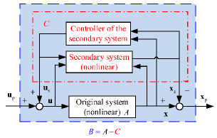
In order to accomplish linearization, the linear system (12) () can be obtained by compensating for the nonlinearity of the original system () using the secondary system () and its controller as shown in Fig. 1. The system from the input to the state is linear. In the subsystems (12) and (13), the secondary system (13) is a virtual exact system, which exists only in design. On the other hand, since the sum of the primary system and the secondary system is the original system, all the uncertainties, such as the higher-order unmodeled dynamics of the real system, are left in the primary system. After state compensation linearization, the controller for the linear primary system (12) can be designed as .
Based on the above content, the following theorem about the conditions for state compensation linearization can be stated.
Theorem 1. System (8) can be linearized by state compensation linearization if
i). in the entire space , Assumption 1 is satisfied.
ii). it can be linearizable by Jacobian linearization.
Proof. First, if Condition i) is met, according to Lemma 1, additive state decomposition holds. Next, if system (8) can be linearizable by Jacobian linearization, then the matrices can be obtained, and thus the primary system (12) can be determined. Then, according to additive state decomposition, the secondary system (13) is determined by the original system and the primary system using the rule (6), namely . Next, one can design a controller to stabilize the secondary system. Consequently, by compensating for the nonlinearity of the original system using the secondary system and its controller, the linear system (i.e., the primary system (12)) can be obtained.
State compensation linearization no longer has multiple equilibrium points. Moreover, in state compensation linearization, there are no coordinate transformation or unit transformation. In some sense, can be considered as a part of , and they have the same dimension and unit. Thus, the physical meaning of the states remains the same after state compensation linearization. This property of state compensation linearization is similar to that of Jacobian linearization. In contrast, the new states obtained from feedback linearization have different physical meanings with the original states because of coordinate transformation.
Remark 1. In state compensation linearization, one keeps both ‘linear primary’ and ‘nonlinear secondary’ component systems. Furthermore, it is not necessarily assumed that the secondary system is ‘small’ in some sense. The secondary system may be significant when the original system has a strong nonlinearity. However, what we often do is to stabilize the secondary system so that it does become ‘small’ eventually, leaving one free to work with the primary system. and are said to be equivalent if the nonlinear secondary system can be stabilized by a controller. Then, checking the equivalence means checking whether the system can be stabilized. In that case a nonlinear system is equivalent to the linear system for which can be stabilized. The difference between state compensation linearization and Jacobian linearization is that state compensation linearization does not throw the ‘error’ system in Jacobian linearization away.
Remark 2. In state compensation linearization, one often needs to construct a stabilizing controller for a nonlinear secondary system. Although designing a stabilizing controller may cost some effort, the benefit is also attractive. The nonlinearity in the secondary system can be better considered, and thus better performance can be expected. Besides, because all the uncertainties and the initial value are considered in the primary system, the stabilizing control problem for the secondary system is a stabilizing control problem of an exact nonlinear system with zero initial states, which is often not complicated.
III-C Comparison of the three linearization methods
Although the linearized systems (12) and (9) have the same , the state and input in (12) are and instead of the real state and input and in (9).
Under some specific conditions, state compensation linearization can be transformed into Jacobian linearization. Considering the original system (8) with . In state compensation linearization, let , , then the resulting linearized system is the same as that of Jacobian linearization, namely .
State compensation linearization seems similar to Jacobian linearization. The difference is that the latter drops the higher-order small nonlinear terms directly and Taylor’s expansion holds locally, which determines its approximate and local properties. In contrast, state compensation linearization uses a compensation strategy, which makes state compensation linearization extend to the whole space and become a kind of accurate linearization method. This property is similar to that of feedback linearization. Thus, state compensation linearization combines the advantages of the two linearization methods in some sense.
Along with state compensation linearization, an original control task can be assigned to the linearized primary system and nonlinear secondary system by dividing the original control task into two simpler control tasks. From this perspective, additive state decomposition is also a task-oriented problem decomposition that offers a general way to decompose an original system into several subsystems in charge of simpler subtasks. Thanks to task decomposition, one can design controllers for simpler subtasks more easily than designing a controller for the original task. These controllers can finally be combined to accomplish the original control task. In the following, state compensation linearization applications to nonlinear control design are discussed.
IV State compensation linearization applications to nonlinear control design
Based on the state compensation linearization method in the previous section, a state-compensation-linearization-based control framework for a class of nonlinear systems is proposed in this subsection. State-compensation-linearization-based stabilizing control is discussed in the following for illustration.
IV-A Problem formulation
IV-B Observer design
It should be pointed out that the primary system and the secondary system are virtual systems, which do not exist in practice and just exist in the analysis. Thus, an observer is necessary to provide the variables of the primary system and the secondary system for the later control design. By using the state compensation linearization method, the unknown disturbance and the initial value are assigned in the primary system, and the secondary system is an exact nonlinear system. Thus, the following observer is built based on the secondary system to observe states [19],[21].
Theorem 2. Suppose that is stable, and an observer is designed to estimate , in (12) and (13) as
| (16) | ||||
| (17) |
where and are the estimation of and . Then , .
Proof. Subtracting (16) from (13) results in and , where . Then, considering that is stable, , which implies that . Consequently, by (15), it can be obtained that .
Remark 3. The designed observer is an open-loop observer, in which must be stable. Otherwise, state feedback is needed to obtain a stable . If a closed-loop observer is adopted here, it will be rather difficult to analyze the stability of the closed-loop system consisting of a nonlinear controller and the observer because separation principle does not hold in nonlinear systems.
Remark 4. The initial values and are both assigned as and . If there is an initial value measurement error, it will be assigned to and considered in the primary system in the form of disturbances.
IV-C State-compensation-linearization-based control framework
Based on state compensation linearization, the original system (8) is decomposed into two systems: an LTI system including all disturbances as the primary system, together with the secondary system whose equilibrium point is the origin. Since the states of the primary system and the secondary system can be observed, the original stabilizing problem for the system (8) is correspondingly decomposed into two problems: a stabilizing problem for the nonlinear secondary system (for the nonlinearity compensation objective) and a stabilizing problem for an LTI primary system (for the control objective). Because the primary system is linear, the classical frequency-domain and time-domain methods can be applied, such as lead-lag compensation. Therefore, the original problem turns into two simpler subproblems. The final objective is achieved once the objectives of the two subproblems are achieved.
-
•
Problem 1 Consider the secondary system (13). Design the secondary controller as
(18) such that as , where is a nonlinear function.
After the compensation of the secondary system and its controller (18), one can get a linear system (primary system). Next, just a stabilizing problem for a linear system needs to be considered.
-
•
Problem 2 Consider the primary system (12). Design the primary controller as
(19) such that or as , where H(s) is a stable transfer function, denotes the inverse Laplace transformation, and state feedback matrix .
Remark 5. In the controller (18), the state feedback matrix can be determined by the linear quadratic regulator (LQR) method or the “PID Tuner App” in the Matlab software. Besides, one can use some kind of robust methods to construct a controller for the primary system.
The controller of the original system can be obtained by combing the controllers of the primary system and the secondary system. With the solutions to the two problems in hand, we can state
Theorem 3. For system (8) under Assumptions 1-3, suppose (i) is stable; (ii) Problems 1-2 are solved; (iii) the controller for system (8) is designed as
| (20) |
Then, the state of system (8) satisfies or as .
Proof. It is easy to obtain that and with the observer (16)-(17). Then, since Problem 1 is solved, as . Furthermore, or as with Problem 2 solved. By additive state decomposition, we have or as .
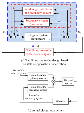
In this new framework, the original problem is simplified, and different control methods are allowed to be applied to the systems. The closed-loop system is shown in Fig. 2. The controller based on state compensation linearization includes three parts: the controller of the primary system, the controller of the secondary system and the observer. In practice, the primary system and the secondary system do not need to have physical status. They are only the models existing in the design.
Remark 6. The basic idea of the state-compensation-linearization-based tracking control framework is similar to that of the state-compensation-linearization-based stabilizing control framework. The most significant difference is that a tracking control problem rather than a stabilizing control problem needs to be specified to the linear primary system.
V Simulation study
In the following, three examples are given to illustrate and compare different linearization methods for control design.
V-A Example 1: A bilinear system
Consider a bilinear system as follows
| (21) |
where represent the state, output, input and disturbance, respectively. It is assumed that . The tracking control goal is to make as .
V-A1 Jacobian-linearization-based-control (JLC) and feedback-linearization-based control (FLC)
The two existing linearization methods are attempted to linearize system (21) so that the given tracking control goal can be achieved by using linear control methods. When the Jacobian linearization method is applied, the first thing is to obtain equilibrium points of system (21). Unfortunately, the stability property of the nonlinear system (21) is affected by the disturbance , which is unknown. Additionally, can be arbitrary values when . This implies that equilibrium points of system (21) cannot be obtained. Without equilibrium points, it is impossible to linearize system (21) by Taylor’s expansion. When the feedback linearization method is applied, let . Then, . There exists a singularity problem that system (21) becomes uncontrollable [26] when . Thus, neither of the two existing linearization methods is suitable for the bilinear system.
V-A2 State-compensation-linearization-based control (SCLC)
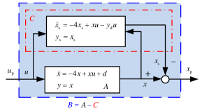
Considering the two existing linearization methods are not readily applicable to system (21), the state compensation linearization method is then adopted. First, a linear primary system () is designed as follows
| (22) |
where let , is the desired output. In the linearization process, because the desired input is unknown, is chosen for simplicity. Then, the following secondary system () is determined by subtracting the primary system (22) from the original system (21) with rule (6)
| (23) |
According to additive state decomposition, it follows
| (24) |
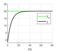
Then, the linear system (22) () can be obtained by compensating for the nonlinearity of the original system (21) () using the secondary system (). The structure is displayed in Fig. 3. If the controller for the primary system (22) is well designed, namely , . Then, the secondary system is approaching the dynamics of which implies that as long as . The final linear system (22) is independent of system (23). The remaining problem is to design a controller for the linear system (22), for which any linear control methods can be utilized. Noteworthy, the proposed state compensation linearization method can avoid the equilibrium point problem of the Jacobian linearization method and the singularity problem of the feedback linearization method. Let , , A proportional-integral-differential (PID) controller is designed for the primary system (22), and the PID parameters are , which is tuned by the “PID Tuner App” in the Matlab software. The simulation result is displayed in Fig. 4. The output can track the reference output well. It is noticed that due to continuity, goes from to , namely at a certain time. This will make feedback linearization fail.
V-B Example 2: An NMP system with saturation
Consider an NMP system with input saturation as follows
| (25) |
with
The saturation function sat is defined as
The system state is measurable. The control objective is to design such that tracks . Next, SCLC is adopted. System (25) can be decomposed into a linear primary system
| (26) |
and a nonlinear secondary system
| (27) |
where let . According to additive state decomposition, it follows
| (28) |
Then, the linear system (26) () can be obtained by compensating for the nonlinearity of the original system (25) () using the secondary system (). If the controller for the primary system (26) is well designed, sat, , which also implies . Then, sat. In this case, since is stable, the secondary system (27) can stabilize itself. The remaining problem is to design a tracking controller for (26) without saturation. By using state compensation linearization and the remaining tracking controller for (26), can hold globally. Let and
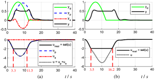
With a PID controller (the PID parameters are , which is tuned by the “PID Tuner App” in the Matlab software) designed for the primary system (26), the simulation result is displayed in Fig. 5(a). The simulation result of JLC is shown in Fig. 5(b) for comparison. For the SCLC, the system undergoes input saturation from s to s (7.2s duration); for the JLC, with the same PID controller, the system undergoes input saturation from s to s (12.7s duration). It can be seen that the SCLC can exit saturation earlier than the JLC and can achieve better tracking performance. In terms of FLC, because the saturation function is irreversible, the real input cannot be obtained. Moreover, because system (25) is an NMP system, FLC may lead to an unstable controller.
V-C Example 3: A mismatched nonlinear system
Consider a mismatched nonlinear system as follows
| (29) |
where is the state, is the input, is the initial state value, and represents the unknown uncertainties.
V-C1 SCLC
Based on the proposed state compensation linearization, for the original system (29), the linear primary system (12) is chosen as
| (30) |
Its state-space form is with
Then, the secondary system (13) can be obtained as
| (31) |
Next, controller design is carried out. For (30), the LQR method is employed to calculate a feedback matrix , and a controller is designed as
For (31), a backstepping controller is designed as
where , , are parameters to be specified later. By combining the two controllers, the final controller follows
V-C2 JLC for comparison
By using Jacobian linearization, the following linearized system is obtained
| (32) |
Its state-space form is with
Based on the linear system (32), a controller is designed as
V-C3 FLC for comparison
By using feedback linearization, the following linearized system is obtained
| (33) |
where , is the virtual input. Its state-space form is with
Based on the linear system (33), a controller is designed as
Then
A singularity problem may be encountered that the system becomes uncontrollable and the control input tends to infinity when ···, i.e., .
V-C4 Robust-Feedback-linearization-based control (RFLC) for comparison
By using robust feedback linearization, the following linearized system is obtained
| (34) |
where . Its state-space form is with
Based on the linear system (34), a controller is designed as
Then
Note that, similarly to FLC, a singularity problem may be encountered.
V-C5 ADRC for comparison [27, 28]
By using ADRC, the following linearized system is obtained
| (35) |
where is the estimation of . Its state-space form is with
The extended state is
An linear extended state observer (LESO) is designed as
where the parameter can be specified later. Then, a controller is designed as
| (36) |
where is designed based on (35) as
It can be seen from (35) that must be reversible. However, in this example, is the estimation of , and thus is irreversible when ···, i.e., . It can be concluded that, similarly to FLC and RFLC, a singularity problem may also be encountered.
V-C6 Simulation results
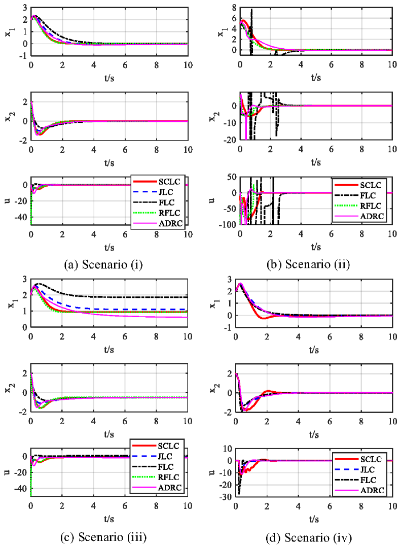
The LQR method is utilized to determine the feedback matrix for all the five control design methods and the parameters are all selected as , . Besides, let , , .
The following four scenarios are presented in the simulation to evaluate and compare the performance of our approach with other linearization methods.
(i) , .
(ii) , .
(iii) , .
(iv) , , a time delay is added into the input channel of the system (29).
Two commonly-used performance indices: the integral absolute error (IAE) and the integral of time-weighted absolute error (ITAE) are used to evaluate the performance of the above five methods quantitatively. Please refer to [29] to find the computation method of IAE and ITAE.
In Scenario (i), the corresponding state and input response is depicted in Fig. 6(a), which shows that all the five methods can achieve stabilization control. Note that the inputs of FLC and RFLC have large initial values. From Tab. I, it can be seen that RFLC has the smallest IAE and ITAE values, which is followed by SCLC in the second place. In Scenario (ii), when the initial state is increased to , the corresponding state and input response is displayed in Fig. 6(b). JLC causes instability and is thus not included in the figure. It can be found that a singularity phenomenon is incurred by FLC, while SCLC still works well. RFLC still has large initial input values. In Scenario (iii), a constant disturbance is considered. From Fig. 6(c) and Tab. I, one can observe that ADRC has the best performance. SCLC also performs well. In Scenario (iv), RFLC causes instability because of the singularity problem and thus do not included in Fig. 6(d). Tab. I shows that SCLC has the best performance.
It can be concluded that, for system (29), JLC has a local property, and causes instability under large initial state values. FLC has a singularity problem and does not have enough robustness. In order to avoid the singularity condition, the working state of the system must be restricted. RFLC has better robustness than FLC. ADRC can tackle unknown disturbances better. However, RFLC and ADRC also have a singularity problem (Some other simulations have also be done where instability is incurred by the singularity problem in RFLC and ADRC, especially when the initial values are large). By contrast, SCLC avoids the local property of JLC, has better robustness than FLC, and avoids the singularity problem in FLC, RFLC, and ADRC. Besides, SCLC can accommodate the input time delay better. This is because all the input time delay is allocated into the primary system by using state compensation linearization. The secondary system deals with the known nonlinearity without the effect of the input time delay. The special strategy mitigates the effect of input time delay on the system. Thus, state compensation linearization can be complementary to the existing linearization methods. For some control problems, if the existing linearization methods do not work well, SCLC is worth trying. The simulation results verify the theoretical conclusion well.
| Sce. | Index | SCLC | JLC | FLC | RFLC | ADRC |
| (i) | IAE | 1.915 | 2.495 | 3.485 | 1.762 | 2.788 |
| ITAE | 1.055 | 1.851 | 3.842 | 0.947 | 4.719 | |
| (ii) | IAE | 5.026 | - | 12.438 | 3.695 | 5.409 |
| ITAE | 2.866 | - | 16.546 | 1.960 | 6.840 | |
| (iii) | IAE | 10.908 | 13.129 | 20.027 | 10.485 | 9.626 |
| ITAE | 48.440 | 57.575 | 95.280 | 47.286 | 36.893 | |
| (iv) | IAE | 2.324 | 2.906 | 2.765 | - | 3.466 |
| ITAE | 1.445 | 2.223 | 2.577 | - | 6.018 |
VI Conclusions
By virtue of additive state decomposition, this paper proposes a new linearization process for control design, namely state compensation linearization. The nonlinear terms can be removed from the original system through the compensation at the input and state so that a linear primary system can be obtained. For some control problems like flight control design with challenging aircraft dynamics, the state compensation linearization may offer some advantages over traditional Jacobian linearization and feedback linearization by bridging the gap between linear control theories and nonlinear systems. Based on the proposed state compensation linearization, this paper proposes a control framework for a class of nonlinear systems so that their closed-loop behavior can follow a specified linear system. Three examples are provided to show the concrete design procedure. Simulation results have illustrated that state-compensation-linearization-based control outperforms Jacobian-linearization-based control and feedback-linearization-based control in some challenging cases. In future research, state-compensation-linearization-based stability margin analysis for nonlinear systems would be considered.
References
- [1] D. M. Wolpert, R. C. Miall, and M. Kawato, “Internal models in the cerebellum,” Trends in Cognitive Sciences, vol. 2, no. 9, pp. 338–347, 1998.
- [2] M. Seigler, S. Wang, S. Koushkbaghi, and J. B. Hoagg, “On the control strategies that humans use to interact with linear systems with output nonlinearities,” in 2018 IEEE International Conference on Systems, Man, and Cybernetics (SMC). IEEE, 2018, pp. 3732–3737.
- [3] H. K. Khalil, Nonlinear systems. Upper Saddle River, NJ: Prentice hall, 2002.
- [4] J.-J. E. Slotine and W. Li, Applied nonlinear control. Englewood Cliffs, NJ: Prentice hall, 1991.
- [5] B. Jakubczyk, W. Respondek et al., “On linearization of control systems,” Bull.acad.pol.sci.ser.sci.math, vol. 28, no. 9-10, pp. 517–522, 1980.
- [6] C.-T. Chen, Introduction to linear system theory. Holt, Rinehart and Winston, 1970.
- [7] R. Chi, Y. Hui, B. Huang, and Z. Hou, “Adjacent-agent dynamic linearization-based iterative learning formation control,” IEEE Transactions on Cybernetics, vol. 50, no. 10, pp. 4358–4369, 2020.
- [8] Q. Gan and C. J. Harris, “Linearization and state estimation of unknown discrete-time nonlinear dynamic systems using recurrent neurofuzzy networks,” IEEE Transactions on Systems, Man, and Cybernetics, Part B (Cybernetics), vol. 29, no. 6, pp. 802–817, 1999.
- [9] X. Peng, K. Guo, X. Li, and Z. Geng, “Cooperative moving-target enclosing control for multiple nonholonomic vehicles using feedback linearization approach,” IEEE Transactions on Systems, Man, and Cybernetics: Systems, vol. 51, no. 8, pp. 4929–4935, 2021.
- [10] A. Alasty and H. Salarieh, “Nonlinear feedback control of chaotic pendulum in presence of saturation effect,” Chaos, Solitons and Fractals, vol. 31, no. 2, pp. 292–304, 2007.
- [11] H. Guillard and H. Bourles, “Robust feedback linearization,” in Proceedings of the 14th International Symposium on Mathematical Theory of Networks and Systems, 2000, pp. 1009–1014.
- [12] J. de Jesús Rubio, “Robust feedback linearization for nonlinear processes control,” ISA transactions, vol. 74, pp. 155–164, 2018.
- [13] A.-C. Huang and S.-Y. Yu, “Input-output feedback linearization control of uncertain systems using function approximation techniques,” in 2016 12th World Congress on Intelligent Control and Automation (WCICA). IEEE, 2016, pp. 132–137.
- [14] J. Umlauft, T. Beckers, M. Kimmel, and S. Hirche, “Feedback linearization using gaussian processes,” in 2017 IEEE 56th Annual Conference on Decision and Control (CDC). IEEE, 2017, pp. 5249–5255.
- [15] J. Han, “From PID to active disturbance rejection control,” IEEE Transactions on Industrial Electronics, vol. 56, no. 3, pp. 900–906, 2009.
- [16] W.-H. Chen, J. Yang, L. Guo, and S. Li, “Disturbance-observer-based control and related methods-An overview,” IEEE Transactions on Industrial Electronics, vol. 63, no. 2, pp. 1083–1095, 2015.
- [17] G. Qi, X. Li, and Z. Chen, “Problems of extended state observer and proposal of compensation function observer for unknown model and application in UAV,” IEEE Transactions on Systems, Man, and Cybernetics: Systems, vol. 52, no. 5, pp. 2899–2910, 2022.
- [18] A. Liu, W.-A. Zhang, L. Yu, H. Yan, and R. Zhang, “Formation control of multiple mobile robots incorporating an extended state observer and distributed model predictive approach,” IEEE Transactions on Systems, Man, and Cybernetics: Systems, vol. 50, no. 11, pp. 4587–4597, 2020.
- [19] Q. Quan, K.-Y. Cai, and H. Lin, “Additive-state-decomposition-based tracking control framework for a class of nonminimum phase systems with measurable nonlinearities and unknown disturbances,” International Journal of Robust and Nonlinear Control, vol. 25, no. 2, pp. 163–178, 2015.
- [20] Z.-B. Wei, Q. Quan, and K.-Y. Cai, “Output feedback ILC for a class of nonminimum phase nonlinear systems with input saturation: An additive-state-decomposition-based method,” IEEE Transactions on Automatic Control, vol. 62, no. 1, pp. 502–508, 2016.
- [21] Q. Quan, H. Lin, and K.-Y. Cai, “Output feedback tracking control by additive state decomposition for a class of uncertain systems,” International Journal of Systems Science, vol. 45, no. 9, pp. 1799–1813, 2014.
- [22] Q. Quan and K.-Y. Cai, “Additive decomposition and its applications to internal-model-based tracking,” in Proceedings of the 48h IEEE Conference on Decision and Control (CDC) held jointly with 2009 28th Chinese Control Conference. IEEE, 2009, pp. 817–822.
- [23] R. A. Nichols, R. T. Reichert, and W. J. Rugh, “Gain scheduling for H-infinity controllers: A flight control example,” IEEE Transactions on Control Systems Technology, vol. 1, no. 2, pp. 69–79, 1993.
- [24] D. J. Leith and W. E. Leithead, “Survey of gain-scheduling analysis and design,” International Journal of Control, vol. 73, no. 11, pp. 1001–1025, 2000.
- [25] Y. Liu, J. J. Zhu, R. L. Williams II, and J. Wu, “Omni-directional mobile robot controller based on trajectory linearization,” Robotics and Autonomous Systems, vol. 56, no. 5, pp. 461–479, 2008.
- [26] L. Tie, “On controllability and near-controllability of discrete-time inhomogeneous bilinear systems without drift,” Automatica, vol. 50, no. 7, pp. 1898–1908, 2014.
- [27] Y. Huang and W. Xue, “Active disturbance rejection control: Methodology and theoretical analysis,” ISA transactions, vol. 53, no. 4, pp. 963–976, 2014.
- [28] Z. Gao, “Active disturbance rejection control: A paradigm shift in feedback control system design,” in 2006 American Control Conference. IEEE, 2006, pp. 2399–2405.
- [29] L. Oliveira, A. Bento, V. J. Leite, and F. Gomide, “Evolving granular feedback linearization: Design, analysis, and applications,” Applied Soft Computing, vol. 86, p. 105927, 2020.