Present address: ]Leibniz-Institut für Polymerforschung Dresden e. V., Institut Theorie der Polymere, Hohe Straße 6, 01069 Dresden, Germany.
Stationary mass distribution and nonlocality in models of coalescence and shattering
Abstract
We study the asymptotic properties of the steady state mass distribution for a class of collision kernels in an aggregation-shattering model in the limit of small shattering probabilities. It is shown that the exponents characterizing the large and small mass asymptotic behavior of the mass distribution depend on whether the collision kernel is local (the aggregation mass flux is essentially generated by collisions between particles of similar masses), or non-local (collision between particles of widely different masses give the main contribution to the mass flux). We show that the non-local regime is further divided into two sub-regimes corresponding to weak and strong non-locality. We also observe that at the boundaries between the local and non-local regimes, the mass distribution acquires logarithmic corrections to scaling and calculate these corrections. Exact solutions for special kernels and numerical simulations are used to validate some non-rigorous steps used in the analysis. Our results show that for local kernels, the scaling solutions carry a constant flux of mass due to aggregation, whereas for the non-local case there is a correction to the constant flux exponent. Our results suggest that for general scale-invariant kernels, the universality classes of mass distributions are labeled by two parameters: the homogeneity degree of the kernel and one further number measuring the degree of the non-locality of the kernel.
pacs:
82.30.Nr, 82.30.Lp, 47.57.eb, 05.70.LnI Introduction
Many-body systems controlled by coalescence arise in many branches of science. The microscopic particles constituting such systems have a tendency to merge irreversibly upon collision or contact. Some examples include hydrogels for biomedical applications Berger et al. (2004), supramolecular polymer gels Sangeetha and Maitra (2005), aerosol formation Friedlander (2000), cloud formation Falkovich et al. (2002); Horvai et al. (2008), ductile fracture Pineau et al. (2016), and charged biopolymers Tom et al. (2016, 2017). By understanding the kinetics of coalescence, the macroscopic properties of such systems can be related to the microphysics of the fundamental collision and merging processes. For more applications and known results see the reviews Leyvraz (2003); Connaughton et al. (2010). In some applications, colliding particles may also fragment or shatter into smaller particles. Whether the collision between particles will result in coagulation or fragmentation of the constituent particles depends on the energy of the colliding particles Wada et al. (2009); Brilliantov et al. (2009). Typically particles with higher kinetic energy fragment, while slow moving ones coalesce or rebound. The size distribution of the fragmented particles is typically a power law distribution Nakamura and Fujiwara (1991); Giblin et al. (1998); Arakawa (1999); Kun et al. (2006), reproducible in simple tractable models Spahn et al. (2014); Dhar (2015). Such fragmentation processes find application in geophysics Grady and Lipkin (1980), astrophysics Michel et al. (2003); Nakamura et al. (2008), glacier modeling Åström et al. (2014), etc.
In this paper we are interested in situations where both coalescence and collisional fragmentation are simultaneously relevant. Examples include the fluctuations of phase coherent domains in high-temperature superconductors Johnson et al. (2011), the statistical properties of insurgent conflicts Bohorquez et al. (2009), the dynamics of herding behavior in financial markets Teh and Cheong (2016), and the formation and stability of planetary rings Davis et al. (1984); Longaretti (1989) where a coalescence–fragmentation model has recently been proposed to explain the particle size distribution of Saturn’s rings over several orders of magnitude Brilliantov et al. (2009, 2015). When coalescence and fragmentation occur together, one might expect the system to reach a nonequilibrium steady state in which the depletion of smaller particles due to coalescence is balanced by the depletion of larger particles due to fragmentation. These nonequilibrium states are expected to be insensitive to fine details of aggregation-fragmentation processes provided that the mass scales at which fragmentation acts as an effective source of light particles and the sink of heavy particles are widely separated. The simplest model of fragmentation for which the described scale separation occurs naturally is such that all fragmented particles are of the size of the smallest possible particle Brilliantov et al. (2009, 2015). We refer to such extreme fragmentation as shattering and use to denote the mass of the smallest particles generated. The expected universality of coalescence-shattering models explains the diversity of their applications and motivates a parametric study of how the particle size distribution depends on the form of the collision kernel, . The kernel depends on the nature of particle motion and interaction and gives the dependence of the microscopic collision rate on the masses, and of the colliding particles.
A particularly important class of collision kernels are homogeneous functions describing collisions that do not have a characteristic mass scale. This class includes many scientifically relevant cases, including the previously mentioned examples. We therefore restrict our attention to homogeneous kernels and denote the degree of homogeneity by . Let us now consider how the stationary mass distribution should scale for a general homogeneous kernel. In the limit of small shattering probability , there is a divergent mass scale beyond which there are very few heavy particles due to a high cumulative probability of shattering. For a large range of masses , we expect to be such that the flux of mass due to coalescence is independent due to local mass conservation. In the well-mixed limit, the mass scaling of the flux can be determined from the following mean field scaling, (see Connaughton et al. (2004) for details):
Constant aggregation flux, , implies that
| (1) |
By analogy with wave turbulence, we refer to the scaling exponent as the Kolmogorov-Zakharov or constant flux exponent. It depends only on the kernel homogeneity, , and therefore possesses a high degree of universality. In particular, it will not change if we perturb the kernel while preserving the value of or change the nature of of sinks and sources (e. g., by removing heavy particles from the system once they become heavier than a fixed mass as in Connaughton et al. (2004) or removing colliding particles at a certain rate as in Connaughton et al. (2017)).
It is natural to ask when these constant flux solution is realized? This question can be answered by substituting the scaling solution as in Eq. (1) into the analytic integral expression for the flux and checking that it remains finite in the limit of small shattering probability (see Refs. Connaughton et al. (2004, 2008) for details of the derivation). It turns out that the realizability of constant flux solution depends on the locality of the collision mechanism. To characterize locality carefully, let us further reduce the class of kernels we are studying by assuming that in addition to having homogeneity degree , has the following asymptotic scaling when one of the colliding particles is much heavier than the other:
Clearly, . This second reduction of generality is as natural for scale-free kernels as the homogeneity. It turns out that the realizabiliity of the Kolmogorov-Zakharov scaling depends, not on , but on the difference
which we call the locality exponent. In Connaughton et al. (2004), we showed that for pure coalescence, the constant flux scaling (1) is realized if the locality exponent . Physically, kernels with lead to the flux of mass due to coalescence being dominated by collisions between similar mass particles. Hence the term “locality.” For pure coalescence, the scaling of the particle size distribution for local kernels is strongly universal: when the characteristic scales of the source and sink are widely separated, it becomes independent of their details and depends only on the degree of homogeneity, , of the collision kernel. We therefore expect intuitively that for the coalescence-fragmentation case with , the scaling of the particle size distribution in the limit of small shattering probability is given by the constant flux expression (1).
This paper confirms this intuition and addresses the nonlocal case, . We will use the simplest family of collision kernels labeled by two exponents and (or equivalently by and ):
| (2) |
Without loss of generality, we assume that . This family has been widely used in general studies of aggregation (see Refs. Leyvraz (2003); Connaughton et al. (2010) for a review). Furthermore, we will always assume that the mean field approximation is applicable, which will allow us to calculate the mass distribution by deriving and solving the corresponding Smoluchowski equation Smoluchowski (1917).
For the family of kernels (2) we will show that if , the scaling exponent of the mass distribution in the limit of small shattering probability is both - and dependent. Moreover, this dependence is different depending on whether (weak non-locality) or (strong non-locality). The amplitude of the mass distribution in the non-local regime is non-universal in the sense that it depends on the effective shattering scale and the mass of dust particles. It is interesting to note that these results for the aggregation-shattering model which conserves mass, parallel the answers for a non-conserved system with coalescence, input of small particles, and collision-dependent evaporation studied in Connaughton et al. (2017). It seems that fine details of the mechanisms leading to effective sources and sinks of particles are irrelevant for a large class of coalescent models even in the non-local regime. An important conclusion from our analysis is that the mass distribution for the model kernel (2) for is different from the mass distribution for the local kernel with the same degree of homogeneity.
The paper is organized as follows. In Sec. II we define the model precisely and state our main quantitative results. In Sec. III we discuss the numerical algorithm that we use to solve for the steady state mass distribution. It is an iterative procedure that we show to reproduce known exact solutions. In Sec. IV we solve the model exactly for two special cases: first when () and second the addition model in which two particles coalesce only when at least one particle is a monomer (). These exact solutions help us to benchmark the numerical algorithm. It is possible to obtain exact results for all integer ’s. This is discussed in Sec. V, where the presence of logarithmic corrections is established for some values of . In Sec. VI, the small mass behavior of the mass distribution is studied using the exact relations between different moments. This enables us to determine the exponents when the kernel is local, and relations between the exponents when the kernel is non-local. In Sec. VII, we analyze the large mass behavior of the mass distribution by studying the singularities of the generating functions. By stitching together the small and large mass behavior, we are able to determine both the small and large mass asymptotic behavior of the mass distribution. In Sec. VIII we discuss the implications of our findings for the specific case of planetary rings since it is an interesting example where both local and nonlocal cases may be relevant. Finally, we conclude with a overview of results and directions of future research in Sec. IX.
II Model
Consider a collection of particles, each characterized by a single scalar parameter, mass. The mass of particle will be denoted by , , and will be measured in terms of the smallest possible mass in the system , corresponding to the smallest possible dust particle, such that is an integer. Given a certain initial configuration, the system evolves in time via coagulation and collision-dependent fragmentation. Two particles of masses and collide at rate , where is the collision kernel. On collision, with probability , the two particles coalesce to form a particle of mass , and with probability , fragment into particles of mass . Note that both the dynamical processes conserve mass, so that total mass is a constant of motion. We would be interested in the limiting case when the fragmentation rate tends to zero, i.e., . Also, we will be considering the well-mixed mean field limit when the spatial correlations between the particles may be neglected.
Let denote the number of particles or mass per unit volume at time . In the well-mixed dilute limit, the time evolution of is described by the Smoluchowski equation:
| (3) |
The first term in the right hand side of Eq. (3) is a gain term that accounts for the number of ways a particle of mass may be created through a coalescence event. The second term is a loss term that accounts for the number of ways in which decreases due to coalescence or fragmentation. The last term describes the creation of particles of mass due to fragmentation events. It is easy to check that the mean mass density is conserved. In this paper, we will be interested in the steady state solution of Eq. (3) obtained by setting the time derivative to . We will denote the steady state solution by . satisfies the equation
| (4) |
We consider the general class of kernels given by
| (5) |
The kernel may also be classified using two other exponents. The first is the homogeneity exponent defined through :
| (6) |
The second is the nonlocality exponent defined as
| (7) |
When , the kernel is referred to as a gelling kernel and non-gelling otherwise. We will refer to kernels with as local kernels and non-local otherwise.
We also consider another kernel that corresponds to the so called addition model Hendriks and Ernst (1984); Brilliantov and Krapivsky (1991); Laurençot (1999); Ball et al. (2011); Blackman and Marshall (1994); Chávez et al. (1997) . Here collision events are allowed only if at least one of the particles has mass . The kernel for the addition model is
| (8) |
which is characterized by a single exponent . This kernel turns out to be exactly solvable (see Sec. IV.2).
In this paper, we will determine the asymptotic behavior of through analysis of the moments as well as the singularities. Moments and generating function are defined as:
| (9) | ||||
| (10) |
Clearly . Multiplying Eq. (4) by and summing over all , we obtain a relation between moments and generating functions,
| (11) |
We also define the exponents that characterize the mass distribution . We assume that the only relevant mass scale in the problem is the cutoff mass and hence has the scaling form:
| (12) |
where is an exponent and is a scaling function. denotes the cutoff scale below and above which behaves differently. There are two cutoff mass scales in the problem. One is the total mass in the system and the other is the scale introduced by fragmentation. We will be working in the limit when total mass is infinite, but mean density is finite, leaving only one cutoff scale. The divergence of the cutoff mass scale as the fragmentation rate is captured by
| (13) |
where the exponent will depend on the kernel. To characterize the scaling behavior for small and large masses, we introduce four new exponents , , and which are defined as:
| (14) | ||||
| (15) |
The exponential decay for large mass is a conjecture. For , the exponential decay with mass will be supported by exact solutions for special cases and numerical observation for more general cases. Further justification for arbitrary kernels follows from the additivity principle using which it has been argued that, for generic conserved mass models, the mass distribution has an exponential decay Chatterjee et al. (2014); Das et al. (2016). The four exponents are not independent. It is straightforward to obtain from Eq. (12) that
| (16) |
The results obtained in this paper for the different exponent as a function of the exponents and are summarized in Table. 1.
III Numerical Algorithm
In this section, we describe the numerical scheme for obtaining the steady state mass distribution . Solving Eq. (4) in the steady state for , we obtain
| (17) |
For , may be determined from Eq. (4) in the steady state, provided , , and all for are known:
| (18) |
Thus, and determine for .
Consider scaled variables and . In terms of these variables, Eqs. (17) and (18) reduce to
| (19) | |||||
| (20) |
and determine for . The two unknowns, and are not independent and related to each other through Eq. (19).
To determine , we follow an iterative procedure as summarized in the flowchart shown in Fig. 1. We start by assigning a numerical value (close to ) for . is determined from Eq. (19). We then solve for up to a value of for which is larger than a predetermined value ( in our analysis), setting for larger values of . We then check for self consistency, i.e whether is equal to the preassigned value of . We increment in small steps until the self-consistency condition is satisfied to the required precision. In our numerical analysis, we demand that the difference between the assumed and calculated values of should be smaller than .
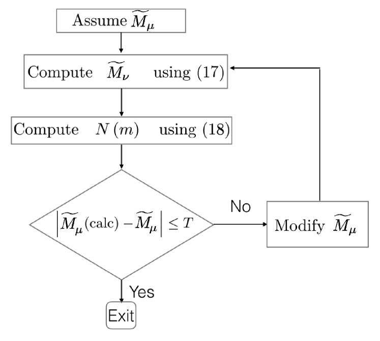
To determine the unscaled variables , we use the fact that mass is conserved: , where will be treated as a parameter. We then scale all by the same factor so that the desired mass density is achieved, thereby determining . In our numerical measurements, we set . There is no proof that the algorithm will result in the convergence of to its correct value. However, we verify the convergence for special solvable kernels (see Sec. IV), leading us to expect that the mass distribution converges to its correct value for more general kernels.
From the numerically computed , we observe that, for all values of and that we have studied, decays exponentially at large masses [as in Eq. (15)]. The exponential cutoff mass is determined by solving for the three parameters (, , and ) in Eq. (15) using for three consecutive ’s and extrapolating to large . Once is determined, the compensated mass distribution is a power law with exponent , allowing us to verify the theoretical results for the exponents at large mass.
IV Exact solutions
The steady state mass distribution may be determined exactly for two cases: (1) when and (2) the addition model (defined in Sec. IV.2).
IV.1 Multiplicative kernel: ()
When , the kernel Eq. (5) reduces to the multiplicative kernel. In this case, Eq. (II) for the generating function reduces to the quadratic equation
| (21) |
which may be solved to yield
| (22) |
where
| (23) |
and the sign of the square root of the discriminant is fixed by the constraint . The coefficient of is the Taylor expansion of is and is:
| (24) |
where
| (25) |
For large , the factorials may be approximated using Stirling formula, and the asymptotic behavior of for large may be derived to be
| (26) |
where
| (27) |
or equivalently the exponent .
In Eq. (26), is determined by the condition that is a constant. It is not possible to find a closed form expression for for arbitrary , however, when is an integer, it is possible to determine it by differentiating or integrating Eq. (22) with respect to and setting . It is then straightforward to obtain for , and for . For generic , we use the asymptotic form Eq. (26) to obtain the dependence of on the cutoff, thus determining . We thus obtain
| (28) |
In the limit of , tends to a finite limit only when the kernel is gelling, i.e., . For non-gelling kernels with , the prefactor tends to zero with decreasing fragmentation rate . This observation may be rationalized by the fact the mass capacity of gelling kernels is finite and infinite for non-gelling kernels. Summarizing the results for , we have derived the results
| (29a) | |||
| (29b) | |||
| (29c) | |||
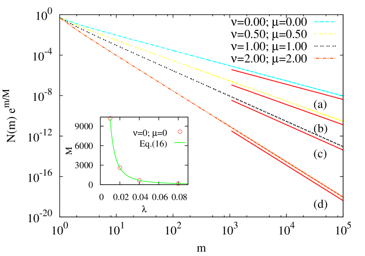
The exact solution for the case can be used to benchmark the numerical scheme described in Sec. III. In Fig. 2, we plot the numerical solution to Eq. (4), obtained using the aforementioned algorithm, for four different values of . The numerically determined cutoff scale is in excellent agreement with the exact solution (see inset of Fig. 2). The data for the compensated mass distribution are power laws with exponents matching the ones obtained from the exact solution (see Fig. 2). We thus conclude that the numerical scheme is accurate and stable.
IV.2 Addition model with fragmentation
In this section, we calculate for the addition model. In this case, collisions between particles are allowed only if at least one of the masses is one, and the resulting collision kernel is as in Eq. (8). While this model is expected to mimic the kernel Eq. (5) with when collisions between dissimilar masses dominate, the exact regime of applicability will become clear only on comparing with the full solution for . For the addition model, the Smoluchowski equation Eq. (4) in the steady state is
| (30) |
This is easily solved to give
| (31) |
which in the limit of large mass and vanishing reduces to
| (32) |
where . The unknown parameter is determined by the constraint that mass is conserved: . We thus obtain
| (33) |
To summarize, we have obtained
| (34a) | |||
| (34b) | |||
| (34c) | |||
for the addition model.
V Mass distribution for integer
It is possible to obtain exact results for the case when the locality exponent is an integer, namely , is an integer. The starting point is Eq. (II). If , where , Eq. (II) reduces to a closed differential equation for :
| (35) |
We expect the singularities to occur at the points in the complex -plane where the coefficient in front of the highest order term is zero. Therefore, at the singular point , satisfies
| (36) |
Introduce new variables as follows:
| (37) | |||||
| (38) |
where and . Then Eq. (V) may be rewritten as
| (39) |
Equation (39) becomes more tractable under the following transformations:
| (40) | |||||
| (41) |
such that we obtain
| (42) |
where
| (43) |
We note that . We now analyze Eq. (42) for specific integer values of .
V.1
When , near the critical point Eq. (42) reduces to
| (44) |
since . Solving for , we obtain
| (45) |
The generating function must be real for , . Therefore we must have or in terms of the original variables,
| (46) |
We conclude that for ,
| (47) |
where the amplitude is
| (48) |
We conclude that in the limit of large masses,
| (49) | |||||
| (50) |
Equivalently,
| (51) |
V.2
When , near the critical point Eq. (42) reduces to
| (54) |
which has a solution given by
where is a positive constant which sets a reference scale in -space. Notice that the solution depends on an arbitrary constant , which is consistent with the solution of a second order ordinary differential equation subject to a single boundary condition . In principle, may be determined by matching this singularity dominated solution with the solution far from the singular point. In the original variables this reads as
| (55) |
where , and
| (56) |
Calculating the jump over the branch cut singularity of , we find that
| (57) |
Changing variables and taking the large- limit of the integral we obtain
| (58) |
where is a reference scale in the mass space.
V.3
Finally, we analyze Eq. (42) for . Near the critical point,
| (61) |
We try the family of solutions:
| (62) |
where is a polynomial of -st degree such that ,
| (63) |
Note that Eq. (62) depends on arbitrary constants [before we impose the condition ], which makes it a good candidate for a general solution. Differentiating the above ansatz, we find:
| (64) |
Substituting this into Eq. (61) gives an answer for the amplitude:
| (65) |
The coefficient can be expressed in terms of : it follows from the definition of that
| (66) |
Applying the inversion formula and using the fact that the analytic part of does not contribute to the large mass asymptotic, one finds that
| (67) |
For small ’s,
| (68) |
The logarithmic corrections to the mass distribution for integer , calculated in this section may be summarized as follows:
| (69) |
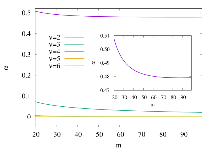
where for and zero otherwise. We also note that these results coincide with the results obtained using analysis of singularities for non-integer [see Eq. (107)]. The solution (69) is now verified using the numerical solution for for integer . Equation (69) has three unknown parameters , , and . These parameters are determined as a function of by using for three consecutive . The variation of with is shown in Fig. 3. In these data, a large value of () is chosen so that the small mass regime is suppressed and the large mass regime is exaggerated. It can be seen from Fig. 3 that the exponents converge, albeit slowly, to their predicted theoretical values [see Eq. (69)].
VI Moment analysis
An exact solution is possible only when . In this section, we use moment analysis to determine some of the exponents characterizing for general and . In particular, we study the small mass behavior of the mass distribution as described by Eq. (14). Our aim is to determine the exponents , , and as a function of and . For this, we will require the equations satisfied by the different moments of . These may be obtained by differentiating Eq. (II) with respect to or by multiplying Eq. (4) by and summing over from to . Doing so gives
| (70) |
which for may be explicitly written as
| (71a) | ||||
| (71b) | ||||
Given the small mass behavior of as in Eq. (14), the dependence of the -th moment of mass on the cutoff mass may be determined as:
| (72) |
where by , we mean that when . There is no divergence at small masses as the integral is cut off at the smallest mass . Thus, we obtain
| (73) |
We first derive upper and lower bounds for the exponent . We first show that . Assume that . We immediately obtain from Eq. (73) that . In this case, Eq. (71a) simplifies to or equivalently . But, is a parameter which tends to 0, hence, we arrive at a contradiction. Hence, . We now show that . Assume . We immediately obtain from Eq. (73) that , and . It is then straightforward to obtain from Eq. (71a) that . Knowing that , Eq. (71b) simplifies to or , in contradiction with the earlier result . Hence, we conclude that .
We now show that . Suppose . Then, from Eq. (73), and for . In this case, Eq. (71b) simplifies to or . But, is a parameter which tends to 0, hence we arrive at a contradiction. Hence, . We now show that . In this case, from Eq. (73), it follows that , , and for . It is straightforward to show that substituting into Eq. (71a) gives , while substituting into Eq. (71b) gives , leading to a contradiction. We thus obtain . Combining the two bounds,
| (74) |
The equations for moments [see Eq. (71)] may be further simplified if only the order of magnitude of the different terms is considered. Consider Eq. (71a). We will argue that the left hand side of Eq. (71a) is dominated by the second term. Let . If the integral (72) determining does not diverge, then neither will the integral for diverge, implying that . Then, . Since , clearly where . On the other hand, if the integral for diverges, then . Then, . Since can diverge utmost as , we again obtain where . Equation (71a) then reduces to , or, equivalently, .
The same reasoning may be used to argue that the left hand side of Eq. (71b) is dominated by the second term. The left hand side is then , where we substituted for . Since [see Eq. (74)], , and the left hand side simplifies to . The right hand side of Eq. (71b) has to be then dominated by . The equations for moments [see Eq. (71)] may then be rewritten as
| (75a) | |||||
| (75b) | |||||
| (75c) | |||||
where Eq. (75b) follows from conservation of mass.
We can now derive , , and in terms of the known parameters. We have already shown that [see Eq. (74)]. For this range of , and applying Eq. (73), we obtain
| (76a) | |||||
| (76b) | |||||
| (76c) | |||||
| (76d) | |||||
Substituting Eq. (76) into Eq. (75), we obtain
| (77a) | ||||
| (77b) | ||||
| (77c) | ||||
To make further progress, we consider different regimes of . Consider first . Equation (77) implies that
| (78a) | |||
| (78b) | |||
| (78c) | |||
where we obtained the constraint on from requiring that a non-zero interval should exist for the inequality satisfied by in Eq. (78c). Note that the values of and cannot be determined using moment analysis alone.
Consider now the second case: . In this regime, Equation (77a) implies that , while Eq. (77c) reduces to
| (79) |
If , then Eq. (79) implies that but we had assumed that . Therefore, we conclude that . This, in conjunction with the assumption , implies that , i.e., the kernel is local. We immediately obtain from Eq. (79) that . Knowing allows to derive all the exponents. To summarize,
| (80a) | |||||
| (80b) | |||||
| (80c) | |||||
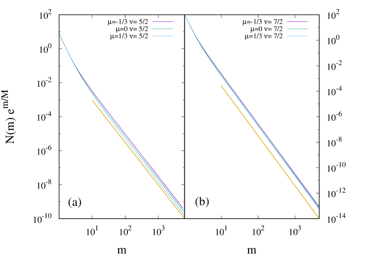
We now verify numerically that the correctness of Eq. (80a) for . In Fig. 4, we show the variation of with for two different values of , and varying . The data for for small masses are independent of , and are consistent with a power law with exponent given by Eq. (80a).
.
Thus when the kernel is local, all exponents describing the small mass behavior of the mass distribution can be obtained using moment analysis, unlike the case when the kernel is non-local. However, the analysis of singularities will enable us to determine the unknown exponents.
We now study the case when , the boundary between the kernel being local or non-local. For this special case, we expect that the power laws will be modified by additional logarithmic corrections Connaughton et al. (2017). We assume the following form for :
| (81) |
where the cutoff mass scale could have a logarithmic dependence on , and and are new exponents that characterize the logarithmic corrections. The choice of is motivated from behavior of Eq. (80a). It is then straightforward to obtain , , and . For , Eq. (75c) reduces to . Substituting for the moments, we immediately obtain
| (82) |
For this choice of , Eq. (75a) immediately yields or
| (83) |
Substituting for the different moments into Eq. (75b), it is straightforward to derive
| (84) | |||||
| (85) |
VII Singularity analysis
In this section, we analyze the equation [see Eq. (II)] satisfied by the generating functions and , based on their singular behavior. This will allow us to determine the exponents and [see Eq. (15) for definition]. This, in turn, will allow us to determine the exponents and characterizing the small mass behavior of for non-local kernels.
Let the singularity of closest to the origin be denoted by . Comparing with Eq. (15), we immediately obtain
| (86) |
Consider , . If the large behavior of is as in Eq. (15), then the leading singular behavior of the generating functions and close to the singular point is proportional to and , respectively. Depending on the value of , or may diverge or tend to a constant as .
Expressing in terms of from Eq. (II), we obtain
| (87) |
We now claim that . Suppose this were not the case and . Then, the denominator in Eq. (87) may be set to a constant when expanding about , and it follows that has the same singular behavior as near . This implies that . When , we have determined the generating function exactly (see Sec. IV), and it is easily seen from Eq. (22) that . This contradicts our initial assumption that . When , and should have different singular singular behavior near , again leading to a contradiction. We therefore conclude that
| (88) |
Expanding the generating functions about , we obtain
| (89a) | |||
| (89b) | |||
where ’s are regular in , , and . Also,
| (90) |
so that Eq. (88) is satisfied. We now examine the numerator of Eq. (87) when . On simplifying by using Eq. (88), it reduces to . However, when . We have shown earlier that for [see Eqs. (78a) and (80c)]. Thus, the numerator of Eq. (87) is non-zero and equal to , when , , and . Substituting the expansions [Eq. (89)] into Eq. (87) we obtain
| (91) |
Since [see Eq. (90)], the right hand side of Eq. (91) diverges. This implies that
| (92) |
and the left hand side of Eq. (91) is dominated by the first term. We can now compare the leading singular behavior on both sides of Eq. (91). There are two possible cases: and .
VII.1
First consider the regime . The denominator of Eq. (91) is dominated by , and comparing the singular terms on both sides, we obtain
| (93) |
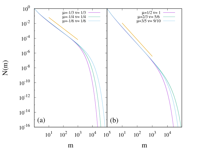
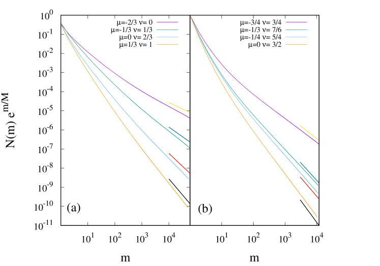
where we obtain the constraint on from our assumption . We now verify numerically that the correctness of Eq. (93) for . In Fig. 5, we show the variation of with for two values of , one between zero and one and the other between one and two, and varying . The data for compensated mass distribution for large masses are consistent with a power law with exponent given by Eq. (93).
Comparing now the coefficients of the leading singular terms we obtain
| (94) |
Once , and are known, and may be obtained from and by doing inverse Laplace transforms. Thus
| (95) | |||||
| (96) |
where is the Gamma function. Multiplying together Eqs. (95), and (96), setting [see Eq. (93)], and using the property
| (97) |
we obtain
| (98) |
for . The prefactor depends on and , which are determined by the behavior of at small masses. Their dependence on the cutoff [see Eq. (76)] will determine :
| (99) |
Knowing [see Eq. (93)], the relation [see Eq. (16)] reduces to
| (100) |
We consider the two cases and separately.
Case I: . In this case, Eq. (100) immediately gives . To satisfy the inequality , we require that . This result for is consistent with what we derived earlier for the local kernel using moment analysis [see Eq. (80a)]. Knowing and [see Eq. (80b)], we obtain from Eq. (99)
| (101) |
Case II: . In this case, Eq. (100) immediately gives
| (102) |
where the constraint on is obtained from the inequality . This result for is consistent with the inequality derived for using moment analysis [see Eq. (78c)], Knowing , , and may be derived from the Eqs. (78b) and (99) to be
| (103) | |||||
| (104) |
For , then there is the possibility of logarithmic corrections.
Thus, we have derived all the exponents characterizing both the small and large mass behavior of when .
VII.2
Consider now the second case when . The denominator of Eq. ((91)) is dominated by . Again comparing the singular terms on both sides of Eq. (91), we obtain
| (105) |
where we obtain the constraint in from our assumption . Comparing the coefficients of the leading singular terms we obtain
| (106) |
It is easy to see that . Doing an inverse Laplace transform, we obtain
| (107) |
The dependence of on may be determined as follows. The integral for has two power laws:
| (108) |
Using the bound Eq. (78c), it is straightforward to argue that to leading order . Substituting and into Eq. (106), we immediately obtain
| (109) |
We consider the two cases and separately.
Case I: . From Eq. (109), we obtain
| (110) |
where the constraint on is obtained from the assumption that . Equation (16) then yields . Therefore, Eqs. (105) and (78b) imply that
| (111) | |||||
| (112) | |||||
| (113) |
Case II: : From Eq. (109), we obtain
| (114) |
This solution in conjunction with our assumption that imply that . But, the solution Eq. (105) is valid only for . Hence there is no solution for this case. We note that the results for and coincide with those for the addition model when [see Eq. (33)] .
We now verify numerically that the correctness of Eq. (111) for . In Fig. 6, we show the variation of with for two values of , for different values of . The data for compensated mass distribution for large masses are consistent with a power law with exponent given by Eq. (111).
VIII Aggregation-fragmentation models for planetary rings
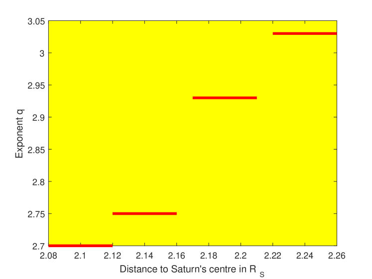
When background stars are occulted by the rings of Saturn, the properties of the scattered light depend on the particle size distribution of the rings. Observation of such occultations suggests a power law distribution of particle sizes. The exponent describing the distribution of particle sizes near the outer edge of the -ring of Saturn extracted from Cassini data in Ref. Becker et al. (2016) varies between and depending on the star occulted. Simple particle models of coalescence and shattering have been proposed to explain the power law scaling. Model-based extractions Zebker et al. (1985) of the scaling exponent suggest an increase in steepness of the distribution with distance to Saturn (see Fig. 7). The graph shows an almost linear increase of the scaling exponent with distance (see Ref. Cuzzi et al. (2010) for an overview and Refs. Brilliantov et al. (2009, 2015) for recent theoretical work). In this section, we discuss the implications of our results for these efforts. In the simplest model it is supposed that binary collisions dominate the dynamics and the collision kernel, depends on the velocity distribution of particles within the rings. The colliding particles coalesce into a single particle of mass with probability and shatter with probability to create ‘dust’ - particles of the smallest mass present in the system. For example, the collision kernel obtained under the assumption of energy equipartition of particles constituting Saturn’s ring is
| (115) |
where is a positive constant. The first mass-dependent factor accounts for the relative particle velocity and the second - for the area of collisional cross section. The homogeneity degree of the kernel (115) is . The rings of Saturn are a non-equilibrium system, therefore, the equipartition of energy does not follow from any general principles. As is suggested in Brilliantov et al. (2015), the whole range of velocity distributions from equipartition of energy to mass-independent root mean square velocity might be present across the different subrings. The latter extreme leads to the following kernel:
| (116) |
which is just proportional to the geometrical cross section. This kernel is also homogeneous with . The kernels (115) and (116) belong to the class of homogeneous kernels described in the Introduction - their asymptotic behavior is captured by exponents and . Studying these kernels when gives and for the kernel (115) and and for the kernel (116). Therefore, for the energy equipartition kernel (115) and for the constant root mean square velocity kernel (116).
Kernel (116) is local and the corresponding distribution of particle masses scales as . This implies that the distribution of particle is given by . The exponent is consistent with the upper range of scaling exponents describing the distribution of constituent sizes in Saturn’s rings Jerousek et al. (2016). On the other hand, the energy equipartition kernel (115) is not local: the substitution of (1) with into the corresponding formula for the flux will lead to a divergence in the limit of small shattering probability. Correspondingly, a conclusion of Brilliantov et al. (2009, 2015) that the mass distribution of particles in the coalescence-shattering model with the kernel (115) scales as (equivalently, the distribution of particle sizes scales as ) is probably incorrect 111The ‘experimental’ curve plotted in Fig. from Brilliantov et al. (2015) does not show raw ‘data from Voyager RSS’. It was obtained in Zebker et al. (1985) using model-based analysis of Voyager occultation data based on a number of assumed model parameters such as the particle’s density. Moreover, the curve does not pertain to the whole A-ring, but just one of its sub-regions (A) where the inferred exponent happens to be . and there is no constant-flux scaling in this case. According to the analysis of Secs. VI and VII in the regime of weak non-locality (), the correct answer for the mass distribution is
| (117) |
Weak non-locality results in -dependent correction to the Kolmogorov-Zakharov exponent. For the kernel (115), this answer means that , or the distribution of particle sizes scales as .
Of course, the exponents and are indistinguishable from the observational point of view given that (i) there are no precise measurements of the spectral exponents for Saturn’s rings (ii) there is no way to fix the parameters of the collision kernel from the existing data on the statistics of particles constituting the rings. By looking at a range of reasonable distributions of velocities of particles in the ring and solving the corresponding Smoluchowski equations the authors of Brilliantov et al. (2015) found the range of scaling exponents describing the distribution of particle sizes to be , which agrees with the numbers accepted by planetary scientists, see e. g. Becker et al. (2016); Jerousek et al. (2016); Colwell et al. (2018). Accounting for the non-locality of the kernel (115), which corresponds to the left boundary of the range, the interval should change to . This is neither here nor there, as the observational knowledge of the exponents is not good enough to distinguish between these predictions. Our conclusions are therefore of a more qualitative nature: the distribution of particles for coalescence-shattering models with homogeneous kernels possessing a well-defined locality exponent is indeed universal in the limit of small shattering probabilities. However, the universality classes are labeled by both the homogeneity degree and the locality exponent rather than by alone as suggested in Brilliantov et al. (2009, 2015). In the local regime, , the dependence of the mass distribution on disappears and we are left with the constant flux distributions (1). For the mass distribution scales with an exponent, which depends on both and . We note that we only describe the universality classes of scaling . The of for non-local kernels is non-universal and depends explicitly on the position of sources and sinks in mass space.
IX Conclusion
In this paper, we determined the steady state mass distribution for a system of particles that on undergoing two-body collisions either coalesce into a single particle or fragment into dust (particles of the smallest mass). The total mass is conserved by the dynamics. Fragmentation acts as a source of particles of small mass while coagulation depletes smaller particles and creates particles of larger mass. We considered a class of homogeneous collision kernels modeled by with , characterized by the homogeneity exponent and non-locality exponent . The results for the exponents characterizing the small and large mass distributions, obtained through a combination of moment analysis, singularity analysis, and exact solutions for special cases, are summarized in Table 1 for different and .
The presence of a non-zero fragmentation rate introduces a cutoff scale beyond which the mass distribution crosses over from a power law behavior to an exponential decay with increasing mass . Thus, a non-zero is a useful regularization scheme by which instantaneous gelation is prevented for kernels that are gelling () and one may study the behavior as the regularization is removed by taking the limit . Here, we find that the form of depends only on whether the kernel is local () or non-local () and not on whether it is gelling or non-gelling.
We find two distinct non-local regimes corresponding to and . When , the distribution is universal in the sense that the small mass behavior does not depend on the source or sink. Thus, the limit is well defined. In the regime, the mass distribution depends on the sink scale but is independent of the source scale, . In the regime , depends on both source and sink. Logarithmic corrections are found at the boundaries between regimes. These are similar to the two non-local regimes that we found for the non-conserved model driven by input of particles at small masses and collision-dependent evaporation Connaughton et al. (2017). The logarithmic corrections are also analogous to the correction proposed by Kraichnan Kraichnan (1971) to account for the marginal non-locality of the enstrophy cascade in two-dimensional fluid turbulence.
As we saw in Sec. VIII, the study of Saturn rings provides examples of both local and non-local kernels. Clearly, there are many open questions relating to the size distribution of ring particles. Can we determine the kernels describing particle collisions in different parts of Saturn’s rings so that more quantitative predictions of particle size distributions can be made? In particular, can the dependence in Fig. 7 be confirmed theoretically? Can one predict regions within the rings of Saturn, where the scaling is of Kolmogorov-Zakharov or constant flux type? Are there regions dominated by weak non-locality or regions correctly described by the addition model? Answering these questions could open up interesting new avenues of research into coalescence-fragmentation models.
Our results also have implications for the addition model in which clusters grow only through reactions with the monomer. The addition model has been studied both as a model for island diffusion though desorption and adsorption of monomers as well as a solvable approximation for more complicated collision kernels Hendriks and Ernst (1984); Brilliantov and Krapivsky (1991); Laurençot (1999); Ball et al. (2011); Blackman and Marshall (1994); Chávez et al. (1997). While the time-dependent as well as steady state solutions have been determined for the addition model, in the latter case, it is not clear when this approximation of restricting collisions only with monomers reproduces the same result as the original kernel. The results of this paper show that for the exponents characterizing the mass distribution for the general kernel coincide with that for addition model for the same . Thus, we conclude that the addition model is a good description of systems with .
In this paper, we studied the steady state but not the dynamics leading to it. This question is important to consider. Even in the local case, , the dynamics leading to the steady state must be very different for gelling () and non-gelling () kernels. Furthermore, in the non-local case, evidence from closely related models Ball et al. (2012, 2011) suggests that the steady state could become unstable for . Such an instability would result in persistent oscillatory kinetics. Indeed, such oscillations have been seen in a recent paper Matveev et al. (2017). This would have interesting consequences for the mass distribution in Saturn rings which could be experimentally verifiable.
In other models of aggregation and fragmentation, where fragmentation occurs spontaneously and not due to a collision, an interesting phase transition occurs when the fragmentation is limited to a finite mass chipping off to a neighbor Majumdar et al. (1998, 2000); Krapivsky and Redner (1996); Rajesh and Majumdar (2001); Rajesh and Krishnamurthy (2002); Rajesh et al. (2002). This model undergoes a nonequilibrium phase transition from a phase in characterized by an exponential mass distribution to a phase characterized by power law mass distribution in the presence of a condensate. The condensate is one single mass which carries a finite fraction of the total mass. It would be interesting to see whether the model considered in the paper exhibits a similar transition in some parameter regimes.
In this paper, we have assumed that the system is well mixed, and hence it was possible to ignore spatial variations in the densities. Also, the effects of stochasticity were completely ignored. Introducing stochasticity, even at the level of zero dimensions, can give rise to new phenomenology like an absorbing-active phase transition in the -density plane. This is because, if total mass is small enough, then the system has a finite probability of getting stuck in an absorbing state where all particles have coalesced into one particle. Including spatial variation would make the problem even richer. This is a promising area for future study.
Acknowledgements.
C.C. and A.D. acknowledge funding from the EPSRC (Grant No. EP/M003620/1). A.D. also thanks the International Centre for Theoretical Sciences (ICTS) for support during a visit for participating in the program -Bangalore School On Statistical Physics - VII (Code No. ICTS/Prog-bssp/2016/07).References
- Berger et al. (2004) J. Berger, M. Reist, J. Mayer, O. Felt, and R. Gurny, Euro. J. Pharma. Biopharma. 57, 35 (2004).
- Sangeetha and Maitra (2005) N. M. Sangeetha and U. Maitra, Chem. Soc. Rev. 34, 821 (2005).
- Friedlander (2000) S. Friedlander, Smoke, Dust, and Haze: Fundamentals of Aerosol Dynamics, Topics in chemical engineering (Oxford University Press, 2000).
- Falkovich et al. (2002) G. Falkovich, A. Fouxon, and M. G. Stepanov, Nature 419, 151 (2002).
- Horvai et al. (2008) P. Horvai, S. V. Nazarenko, and T. H. M. Stein, J. Stat. Phys. 130, 1177 (2008).
- Pineau et al. (2016) A. Pineau, A. A. Benzerga, and T. Pardoen, Acta Mater. 107, 424 (2016).
- Tom et al. (2016) A. M. Tom, R. Rajesh, and S. Vemparala, J. Chem. Phys. 144, 034904 (2016).
- Tom et al. (2017) A. M. Tom, R. Rajesh, and S. Vemparala, J. Chem. Phys. 147, 144903 (2017).
- Leyvraz (2003) F. Leyvraz, Phys. Rep. 383, 95 (2003).
- Connaughton et al. (2010) C. Connaughton, R. Rajesh, and O. Zaboronski, in Handbook of Nanophysics: Clusters and Fullerenes, edited by K. D. Sattler (Taylor and Francis, 2010).
- Wada et al. (2009) K. Wada, H. Tanaka, T. Suyama, H. Kimura, and T. Yamamoto, Astrophys. J. 702, 1490 (2009).
- Brilliantov et al. (2009) N. V. Brilliantov, A. S. Bodrova, and P. L. Krapivsky, J. Stat. Mech. 2009, P06011 (2009).
- Nakamura and Fujiwara (1991) A. Nakamura and A. Fujiwara, Icarus 92, 132 (1991).
- Giblin et al. (1998) I. Giblin, G. Martelli, P. Farinella, P. Paolicchi, M. Di Martino, and P. Smith, Icarus 134, 77 (1998).
- Arakawa (1999) M. Arakawa, Icarus 142, 34 (1999).
- Kun et al. (2006) F. Kun, F. Wittel, H. Herrmann, B. Kröplin, and K. Måløy, Phys. Rev. Lett. 96, 025504 (2006).
- Spahn et al. (2014) F. Spahn, E. V. Neto, A. H. F. Guimarães, A. N. Gorban, and N. V. Brilliantov, New J. Phys. 16, 013031 (2014).
- Dhar (2015) D. Dhar, J. Phys. A 48, 175001 (2015).
- Grady and Lipkin (1980) D. Grady and J. Lipkin, Geophys. Res. Lett. 7, 255 (1980).
- Michel et al. (2003) P. Michel, W. Benz, and D. C. Richardson, Nature 421, 608 (2003).
- Nakamura et al. (2008) A. Nakamura, T. Michikami, N. Hirata, A. Fujiwara, R. Nakamura, M. Ishiguro, H. Miyamoto, H. Demura, K. Hiraoka, T. Honda, C. Honda, J. Saito, T. Hashimoto, and T. Kubota, Earth Planets Space 60, 7 (2008).
- Åström et al. (2014) J. A. Åström, D. Vallot, M. Schäfer, E. Z. Welty, S. O’neel, T. Bartholomaus, Y. Liu, T. Riikilä, T. Zwinger, J. Timonen, and J. C. Moore, Nat. Geosci. 7, 874 (2014).
- Johnson et al. (2011) N. F. Johnson, J. Ashkenazi, Z. Zhao, and L. Quiroga, AIP Advances 1, 012114 (2011).
- Bohorquez et al. (2009) J. C. Bohorquez, S. Gourley, A. R. Dixon, M. Spagat, and N. F. Johnson, Nature 462, 911 (2009).
- Teh and Cheong (2016) B. K. Teh and S. A. Cheong, PloS one 11, e0163842 (2016).
- Davis et al. (1984) D. R. Davis, S. J. Weidenschilling, C. R. Chapman, and R. Greenberg, Science 224, 744 (1984).
- Longaretti (1989) P.-Y. Longaretti, Icarus 81, 51 (1989).
- Brilliantov et al. (2015) N. Brilliantov, P. Krapivsky, A. Bodrova, F. Spahn, H. Hayakawa, V. Stadnichuk, and J. Schmidt, Proc. Nat. Acad. Sci. 112, 9536 (2015).
- Connaughton et al. (2004) C. Connaughton, R. Rajesh, and O. Zaboronski, Phys. Rev. E 69, 061114 (2004).
- Connaughton et al. (2017) C. Connaughton, A. Dutta, R. Rajesh, and O. Zaboronski, Euro. Phys. Lett. 117, 10002 (2017).
- Connaughton et al. (2008) C. Connaughton, R. Rajesh, and O. Zaboronski, Phys. Rev. E 78 (2008).
- Smoluchowski (1917) M. V. Smoluchowski, Z. Phys. Chem. 92, 129 (1917).
- Hendriks and Ernst (1984) E. Hendriks and M. Ernst, J. Coll. Inter. Sci. 97, 176 (1984).
- Brilliantov and Krapivsky (1991) N. V. Brilliantov and P. L. Krapivsky, J. Phys. A 24, 4789 (1991).
- Laurençot (1999) P. Laurençot, Nonlinearity 12, 229 (1999).
- Ball et al. (2011) R. C. Ball, C. Connaughton, T. H. M. Stein, and O. Zaboronski, Phys. Rev. E 84, 011111 (2011).
- Blackman and Marshall (1994) J. Blackman and A. Marshall, J. Phys. A 27, 725 (1994).
- Chávez et al. (1997) F. Chávez, M. Moreau, and L. Vicente, J. Phys. A 30, 6615 (1997).
- Chatterjee et al. (2014) S. Chatterjee, P. Pradhan, and P. Mohanty, Phys. Rev. Lett. 112, 030601 (2014).
- Das et al. (2016) A. Das, S. Chatterjee, and P. Pradhan, Phys. Rev. E 93, 062135 (2016).
- Becker et al. (2016) T. M. Becker, J. E. Colwell, L. W. Esposito, and A. D. Bratcher, Icarus 279, 20 (2016), planetary Rings.
- Zebker et al. (1985) H. A. Zebker, E. A. Marouf, and G. L. Tyler, Icarus 64, 531 (1985).
- Cuzzi et al. (2010) J. N. Cuzzi et al., Science 327, 1470 (2010).
- Jerousek et al. (2016) R. G. Jerousek, J. E. Colwell, L. W. Esposito, P. D. Nicholson, and M. M. Hedman, Icarus 279, 36 (2016).
- Colwell et al. (2018) J. Colwell, L. Esposito, and J. Cooney, Icarus 300, 150 (2018).
- Kraichnan (1971) R. H. Kraichnan, J. Fluid. Mech. 47, 525 (1971).
- Ball et al. (2012) R. C. Ball, C. Connaughton, P. P. Jones, , R. Rajesh, and O. Zaboronski, Phys. Rev. Lett. 109, 168304 (2012).
- Matveev et al. (2017) S. A. Matveev, P. L. Krapivsky, A. P. Smirnov, E. E. Tyrtyshnikov, and N. V. Brilliantov, Phys. Rev. Lett. 119, 260601 (2017).
- Majumdar et al. (1998) S. N. Majumdar, S. Krishnamurthy, and M. Barma, Phys. Rev. Lett 81, 3691 (1998).
- Majumdar et al. (2000) S. N. Majumdar, S. Krishnamurthy, and M. Barma, J. Stat. Phys. 99, 1 (2000).
- Krapivsky and Redner (1996) P. Krapivsky and S. Redner, Phys. Rev. E 54, 3553 (1996).
- Rajesh and Majumdar (2001) R. Rajesh and S. Majumdar, Phys. Rev. E 63, 036114 (2001).
- Rajesh and Krishnamurthy (2002) R. Rajesh and S. Krishnamurthy, Phys. Rev. E 66, 046132 (2002).
- Rajesh et al. (2002) R. Rajesh, D. Das, B. Chakraborty, and M. Barma, Phys. Rev. E 66, 056104 (2002).