Stationary subsonic boundary layer in the regions of local heating of surface

Let us consider the stationary problem. Then (2.2) may be transformed as follows

$$\frac{\partial u_{b}}{\partial x_{b}}+\frac{\partial v_{b}}{\partial y_{b}}=0,$$

$$u_{b}\frac{\partial u_{b}}{\partial x_{b}}+v_{b}\frac{\partial u_{b}}{\partial y_{b}}+T_{b}\frac{\partial p_{b}}{\partial x_{b}}=\frac{\partial^{2}u_{b}}{\partial y_{b}^{2}}$$

(3.1)

$$u_{b}\frac{\partial T_{b}}{\partial x_{b}}+v_{b}\frac{\partial T_{b}}{\partial y_{b}}=\frac{\partial^{2}T_{b}}{\partial y_{b}^{2}}$$

Assume that the temperature disturbances are small i.e., $\Delta T<<T\sim O(1)$. Then the solution of (3.1) may be constructed by expanding the flow functions in the main undisturbed part of the boundary layer. Let us introduce the small parameter $\lambda=\Delta T$ and represent the flow functions as follows

$$u_{b}=y_{b}+\lambda U+O(\lambda^{2}),\quad v_{b}=\lambda V+O(\lambda^{2}),\quad\mathcal{A}_{1b}=\lambda\mathcal{A}_{1}+O(\lambda^{2})$$

$$T_{b}=1+\lambda T+O(\lambda^{2}),\quad p_{b}=\lambda P+O(\lambda^{2}),\quad\mathcal{A}_{b}=\lambda\mathcal{A}+O(\lambda^{2})$$

as $\lambda\to 0$. Substitution of these expansions in (3.1) and boundary condition and equalization of the terms with the same powers of $\lambda$ yield the set

$$\frac{\partial U}{\partial x_{b}}+\frac{\partial V}{\partial y_{b}}=0,$$

$$y_{b}\frac{\partial U}{\partial x_{b}}+V+\frac{\partial P}{\partial x_{b}}=\frac{\partial^{2}U}{\partial y_{b}^{2}}$$

$$y_{b}\frac{\partial T}{\partial x_{b}}=\frac{\partial^{2}T}{\partial y_{b}^{2}}$$

The boundary conditions take the form

$$U(x_{b},0)=V(x_{b},0)=0,T(x_{b},0)=T_{w}(x_{b}),$$

$$U\to\mathcal{A}(x_{b}),\quad\mathcal{A}_{1}(x_{b})=\int_{0}^{+\infty}Td\eta+\mathcal{A}(x_{b}),\quad T(x_{b},\infty)\to 0,y_{b}\to\infty$$

$$\mathcal{A}(-\infty)=0,\quad\mathcal{A}^{\prime\prime}_{1}(x_{b})=-\int\limits_{-\infty}^{+\infty}\frac{P^{\prime}(\xi)}{x_{b}-\xi}d\xi$$

Applying Fourier transform with respect to $x_{b}$ to the last set, we obtain

$$i\xi\tilde{U}+\tilde{V}^{\prime}=0,$$

$$i\xi y_{b}\tilde{U}+\tilde{V}+i\xi\tilde{P}=\tilde{U}^{\prime\prime},$$

(3.2)

$$i\xi y_{b}\tilde{T}=\tilde{T}^{\prime\prime}$$

Consider the last equation of (3.2). Set $Y=(i\xi)^{1/3}y_{b}$ and $y_{b}>0$. Then the equation becomes

$$\tilde{T}^{\prime\prime}=Y\tilde{T},$$

where primes denote differentiating with respect to $Y$. Thus, in the result of variable changing the variable $Y$ is complex and the equation for Fourier image is Airy equation. To determine the values of $Y$ uniquely it is necessary to specify the branch of multi-valued function $(i\xi)^{1/3}$. Let us consider the complex plane $\omega=\eta+i\xi$. We find for Airy function $\operatorname{Ai}(\omega^{1/3}y_{b})$. Cut the plane $\omega$ along the negative part of real half axis. In the plane with the cut the function $\omega^{1/3}$ allows to specify regular branches. Then take the branch of cubic root such that at $\omega=1$ we have $\omega^{1/3}=1$. In the following consideration we will use the consequence of previous procedure, that for the branch under consideration $\operatorname{Ai}((i\xi)^{1/3}y_{b})=\operatorname{Ai}(\xi^{1/3}y_{b}\operatorname{e}^{i\pi/6})$ as $\xi>0$ and $\operatorname{Ai}((i\xi)^{1/3}y_{b})=\operatorname{Ai}(\xi^{1/3}y_{b}\operatorname{e}^{-i\pi/6})$ as $\xi<0$.

The boundary condition at infinity is derived from those for (2.2) and has the form $\tilde{T}(\infty)=0$. The second boundary condition is set using the temperature distribution on the wall and taking into account its Fourier transform and has the form $\tilde{T}(\xi)=\tilde{f}(\xi)$. Using the new variable $Y$ the equation for Fourier images of temperature becomes Airy equation. The boundary condition at infinity shows the solution of Airy equation must be chosen recessive at infinity. This solution depends on $Y$ complex plane segment under consideration. However, the above suggested specification of the branch shows that in the case under consideration the argument of Airy functions is located in the segment defined by $\left|(\right|argY)<\pi/3$ where the recessive solution is represented by means of $Ai(Y)$ and hence the solution is given by

$$\tilde{T}(\xi,y_{b})=K(\xi)\operatorname{Ai}(Y).$$

The boundary condition in zero point gives

$$K(\xi)=\frac{\tilde{f}(\xi)}{\operatorname{Ai}(0)},$$

and we obtain the solution for the images of the temperature.

Consider two other equations of (3.2). Differentiating the second one with respect to $y_{b}$ and substituting the result in the first equation we obtain

$$\tilde{U}^{\prime\prime\prime}=-i\xi y_{b}\tilde{U}^{\prime}.$$

Introducing notation $\tilde{U}^{\prime}=F$ and changing variables as above, i.e. $Y=(i\xi)^{1/3}y_{b}$, we arrive at Airy equation

$$F^{\prime\prime}=YF.$$

In the last equation the primes imply differentiation with respect to $Y$. The boundary condition for this equation follows from the asymptotic relation for the longitudinal velocity as $y_{b}\to+\infty$. The solution of the equation satisfying the boundary condition is represented by Airy function $\operatorname{Ai}(Y)$. The solution also depends on the complex plane segments as in the case of the temperature equation and we do not repeat the above analysis. Notice that the velocity distributions are not crucial functions in the problem under consideration. It is necessary to obtain the wall-shear and the pressure in the viscous sublayer. Thus, we find

$$\tilde{U}^{\prime}(\xi,y_{b})=M(\xi)\operatorname{Ai}(Y).$$

(3.3)

To determine $M(\xi)$ we observe that the longitudinal impulse equation yields at $y_{b}=0$

$$\frac{\partial{P}}{\partial{x_{b}}}=\frac{\partial^{2}{U}}{\partial{y_{b}^{2}}}(x_{b},0).$$

For the pressure derivative we denote $P^{\prime}_{x_{b}}=G(x_{b})$. Then the equation for images takes the form

$$\tilde{G}=\tilde{U}^{\prime\prime}(\xi,0)$$

(3.4)

Differentiating (3.3) with respect to $y_{b}$, evaluating it at $y_{b}=0$ and substituting in (3.4), we have

$$\tilde{G}=M(\xi)(i\xi)^{1/3}\operatorname{Ai}^{\prime}(0).$$

The second necessary relation for evaluating $\tilde{G}$ and $M(\xi)$ follows from the interaction condition and has the form

$$U^{\prime\prime}(x_{b},\infty)+\int\limits_{0}^{+\infty}T^{\prime\prime}d\eta=-\int\limits_{-\infty}^{+\infty}\frac{P^{\prime}(\zeta)}{x_{b}-\zeta}d\zeta$$

Applying the Fourier transform to the last equality, we obtain

$$(i\xi)^{2}\tilde{U}(\xi,\infty)+(i\xi)^{2}\int\limits_{0}^{+\infty}\tilde{T}(\xi,\eta)d\eta=-\int\limits_{-\infty}^{+\infty}\operatorname{e}^{-i\xi x_{b}}dx_{b}\int\limits_{-\infty}^{+\infty}\frac{P^{\prime}(\zeta)}{x_{b}-\zeta}d\zeta=$$

$$=-i\pi\frac{\left|\xi\right|}{\xi}\int\limits_{-\infty}^{+\infty}\operatorname{e}^{-i\xi\zeta}P^{\prime}(\zeta)d\zeta=i\pi\frac{\left|\xi\right|}{\xi}\hat{G}$$

Next, observe that from the foregoing analysis follows

$$\tilde{U}(\xi,\infty)=\frac{M(\xi)}{(i\xi)^{1/3}}\int\limits_{0}^{+\infty}\operatorname{Ai}(z)dz,\quad\tilde{T}=\tilde{f}\frac{\operatorname{Ai}(Y)}{\operatorname{Ai}(0)},$$

we arrive at the following condition

$$\left(i\pi\frac{\left|\xi\right|}{\xi}+\frac{(i\xi)^{4/3}}{k^{4/3}}\right)\tilde{G}=\frac{(i\xi)^{5/3}\tilde{f(\xi)}}{\operatorname{Ai}(0)}\int\limits_{0}^{+\infty}\operatorname{Ai}(z)dz,$$

where we use the notation $k=(-\operatorname{Ai}^{\prime}(0)/\int_{0}^{+\infty}\operatorname{Ai}(z)dz)^{3/4}=0.827$[12]. Here it is necessary to return to the problem of Airy function argument choosing. The last discussion arrive at improper integral of $\operatorname{Ai}(Y)$ calculation which converges as $\left|arg(Y)\right|<\pi/3$[11]. The branch of $\omega^{1/3}$ must be specified to provide the convergence of the integral both as $\xi>0$ and $\xi<0$. The above specified branch provides this convergence.

Taking into account two conditions for $\tilde{G}$ and $M(\xi)$ we obtain

$$\tilde{G}=-\frac{\operatorname{Ai}^{\prime}(0)}{\operatorname{Ai}(0)}\frac{(i\xi)^{5/3}\tilde{f}(\xi)}{\left(i\pi\frac{\left|\xi\right|}{\xi}k^{4/3}+(i\xi)^{4/3}\right)}$$

$$M(\xi)=-\frac{1}{\operatorname{Ai}(0)}\frac{(i\xi)^{4/3}\tilde{f}(\xi)}{\left(i\pi\frac{\left|\xi\right|}{\xi}k^{4/3}+(i\xi)^{4/3}\right)}.$$

Lastly, for the Fourier images of the shear we find from the previous relation

$$\tilde{\tau}=\tilde{U}^{\prime}_{y_{b}}(\xi,0)=M(\xi)\operatorname{Ai}(0)=-\frac{(i\xi)^{4/3}\tilde{f}(\xi)}{\left(i\pi\frac{\left|\xi\right|}{\xi}k^{4/3}+(i\xi)^{4/3}\right)}.$$

In all above formulas the plus is chosen at $\xi>0$ and the minus at $\xi<0$.

The relations for the functions $M(\xi)$ and $\tilde{G}$ show that in the case under consideration the influence of the function $\tilde{f}(\xi)$ on convergence of integrals for the wall-shear and the pressure is more significant than in the supersonic case[13]. It follows that the shape of local heating region has more influence on the functions in the lower-deck than in the supersonic case. Let us note the properties of $\tilde{f}(\xi)$ to be used below. Since we consider the local regions of heating, we assume this function to be Fourier transform of some finite function. Then, the original finite function is assumed to be even, implying its Fourier transform to be a real function. We consider the pressure case in more detail for the below analysis is similar for the wall-shear.

The pressure gradient on the wall is given by

$$P^{\prime}_{x_{b}}=G(x_{b})=-\frac{1}{2\pi}\int\limits_{-\infty}^{+\infty}\tilde{G}(\xi)\operatorname{e}^{i\xi x_{b}}d\xi=$$

$$=-\frac{1}{2\pi}\frac{\operatorname{Ai}^{\prime}(0)}{\operatorname{Ai}(0)}\left[\int\limits_{-\infty}^{0}\frac{(i\xi)^{5/3}\tilde{f}(\xi)}{-i\pi k^{4/3}+(i\xi)^{4/3}}\operatorname{e}^{i\xi x_{b}}d\xi+\int\limits_{0}^{+\infty}\frac{(i\xi)^{5/3}\tilde{f}(\xi)}{i\pi k^{4/3}+(i\xi)^{4/3}}\operatorname{e}^{i\xi x_{b}}d\xi\right].$$

Accomplishing the simple transformations and using the results of §3.1, introducing the variable $r>0$ such that as $\xi>0$ we have $i\xi=r\operatorname{e}^{i\pi/2}$ and as $\xi<0$ $i\xi=r\operatorname{e}^{-i\pi}$, we obtain

$$G(x_{b})=-\frac{1}{2\pi}\frac{\operatorname{Ai}^{\prime}(0)}{\operatorname{Ai}(0)}\left[\int\limits_{0}^{+\infty}\frac{\operatorname{e}^{-i5\pi/6}r^{5/3}\tilde{f}(-r)}{-i\pi k^{4/3}+\operatorname{e}^{-i2\pi/3}r^{4/3}}\operatorname{e}^{-irx_{b}}dr\right.+$$

$$+\left.\int\limits_{0}^{+\infty}\frac{\operatorname{e}^{i5\pi/6}r^{5/3}\tilde{f}(r)}{i\pi k^{4/3}+\operatorname{e}^{i2\pi/3}r^{4/3}}\operatorname{e}^{irx_{b}}dr\right].$$

(3.5)

The heating region of the surface has some length, therefore to estimate the shear and the pressure we set the temperature on the wall by means of the following finite even function

$$T(x_{b},0)=\left\{\begin{aligned} 0.2,&\left|x_{b}\right|\leq 0.5\\ 0,&\left|x_{b}\right|>0.5.\\ \end{aligned}\right.$$

Fourier transform of this function yields

$$\tilde{f}(\xi)=\frac{0.4}{\xi}\sin\left(\frac{\xi}{2}\right).$$

It follows that $\tilde{f}(\xi)\to 0$ as $\xi\to\infty$ and even. In addition, it is easily seen that in (3.5) we obtain the sum of two conjugate functions. Substituting the last relation in (3.5) and taking into account the complex conjugation, we obtain the integral representation of the general solution in the sublayer for the pressure

$$P^{\prime}(x_{b})=-\frac{0.4}{\pi}\frac{\operatorname{Ai}^{\prime}(0)}{\operatorname{Ai}(0)}\int\limits_{0}^{+\infty}\frac{r^{2/3}\sin(rx_{b}-\psi)\sin(r/2)dr}{\sqrt{\pi^{2}k^{8/3}+\sqrt{3}\pi k^{4/3}r^{4/3}+r^{8/3}}},$$

(3.6)

where $\psi$ is determined by

$$\psi=\arctan\left(\frac{\pi k^{4/3}+\sqrt{3}r^{4/3}}{r^{4/3}+\sqrt{3}\pi k^{4/3}}\right)$$

In the similar way for the shear we obtain

$$\frac{\partial{U}}{\partial{y_{b}}}(x_{b},0)=-\frac{0.4}{\pi}\int\limits_{0}^{+\infty}\frac{r^{1/3}\sin(rx_{b}-\phi)\sin(r/2)dr}{\sqrt{\pi^{2}k^{8/3}+\sqrt{3}\pi k^{4/3}r^{4/3}+r^{8/3}}},$$

where

$$\phi=\arctan\left(\frac{\frac{\sqrt{3}}{2}\pi k^{4/3}+r^{4/3}}{\frac{1}{2}\pi k^{4/3}}\right)$$

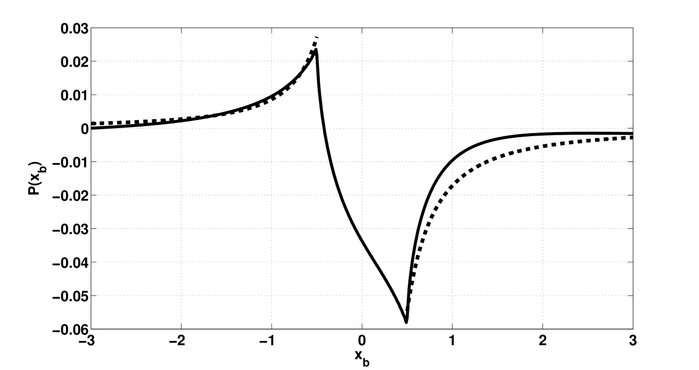
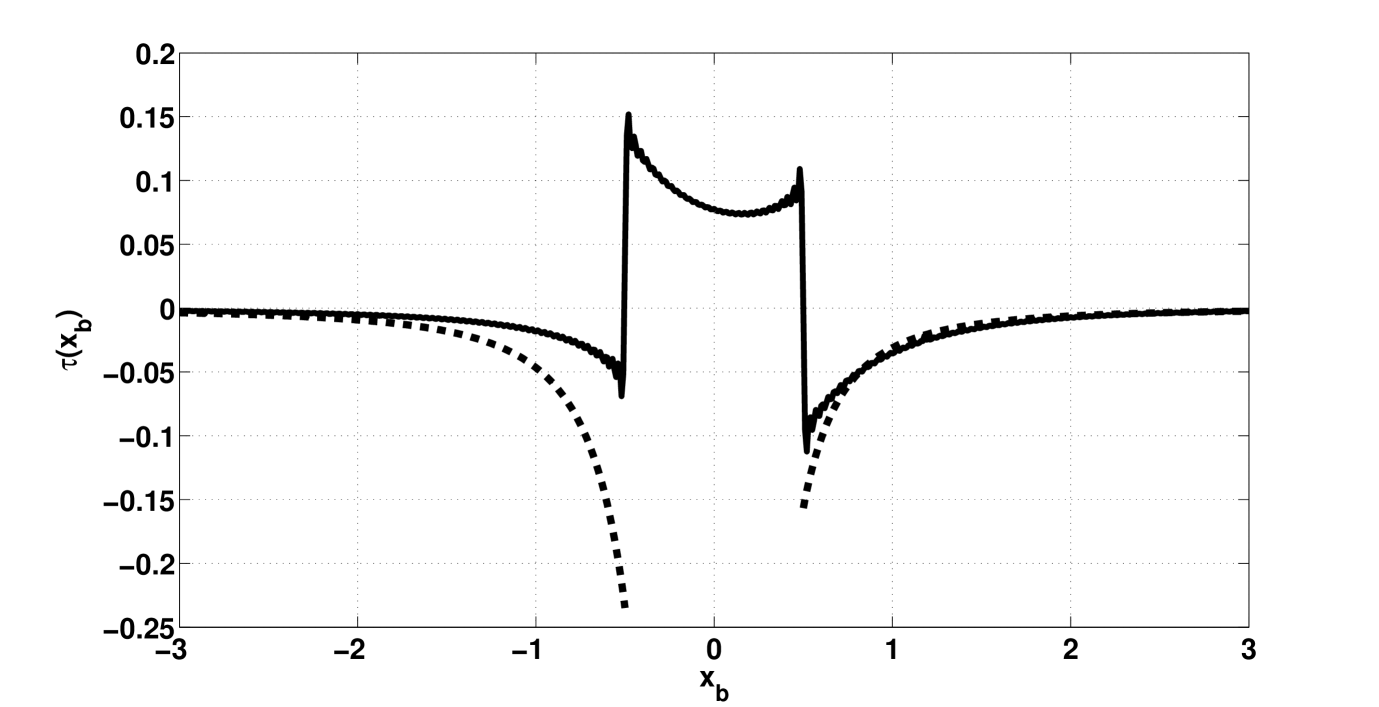
The results of pressure estimation are depicted in fig. 1, and the wall-shear, in fig. 2. The pressure estimation is obtained by means of integration of (3.6).

Let us consider the asymptotic behaviour of flow functions and firstly consider the wall-shear case. The main relation we represent as the sum of integrals as follows

$$\frac{\partial{U}}{\partial{y_{b}}}(x_{b},0)=-\frac{0.4}{\pi}\int\limits_{0}^{+\infty}\frac{r^{1/3}\left(\frac{\sqrt{3}}{2}\pi k^{4/3}+r^{4/3}\right)\sin(r/2)\cos(rx_{b})dr}{\pi^{2}k^{8/3}+\sqrt{3}\pi k^{4/3}r^{4/3}+r^{8/3}}+$$

$$+\frac{0.4}{\pi}\int\limits_{0}^{+\infty}\frac{r^{1/3}\frac{1}{2}\pi k^{4/3}\sin(r/2)\sin(rx_{b})dr}{\pi^{2}k^{8/3}+\sqrt{3}\pi k^{4/3}r^{4/3}+r^{8/3}}=$$

$$=-\frac{0.4}{\pi}\frac{1}{4i}\left[\int\limits_{0}^{+\infty}r^{1/3}h_{1}(r)\operatorname{e}^{ir(x_{b}+1/2)}dr+\int\limits_{0}^{+\infty}r^{1/3}h_{1}(r)\operatorname{e}^{-ir(x_{b}-1/2)}dr-\right.$$

$$-\left.\int\limits_{0}^{+\infty}r^{1/3}h_{1}(r)\operatorname{e}^{ir(x_{b}-1/2)}dr-\int\limits_{0}^{+\infty}r^{1/3}h_{1}(r)\operatorname{e}^{-ir(x_{b}+1/2)}dr\right]-$$

$$+\frac{0.4}{\pi}\frac{1}{4}\left[\int\limits_{0}^{+\infty}r^{1/3}h_{2}(r)\operatorname{e}^{ir(x_{b}+1/2)}dr-\int\limits_{0}^{+\infty}r^{1/3}h_{2}(r)\operatorname{e}^{-ir(x_{b}-1/2)}dr-\right.$$

$$-\left.\int\limits_{0}^{+\infty}r^{1/3}h_{2}(r)\operatorname{e}^{ir(x_{b}-1/2)}dr+\int\limits_{0}^{+\infty}r^{1/3}h_{2}(r)\operatorname{e}^{-ir(x_{b}+1/2)}dr\right],$$

where we use the following notation

$$h_{1}(r)=\frac{\frac{\sqrt{3}}{2}\pi k^{4/3}+r^{4/3}}{\pi^{2}k^{8/3}+\sqrt{3}\pi k^{4/3}r^{4/3}+r^{8/3}},\quad h_{2}(r)=\frac{\frac{1}{2}\pi k^{4/3}}{\pi^{2}k^{8/3}+\sqrt{3}\pi k^{4/3}r^{4/3}+r^{8/3}}.$$

Observe that

$$h_{1}(0)=\frac{\sqrt{3}}{2}\pi k^{4/3},\quad h_{2}(0)=\frac{1}{2}\pi k^{4/3},\quad h^{\prime}_{1}(0)=h^{\prime}_{2}(0)=0.$$

For the above integrals the asymptotic relations as $x_{b}\to+\infty$ can be given being the specific case of relations described in [14], namely

$$\int\limits_{0}^{+\infty}r^{1/3}h(r)\operatorname{e}^{\pm ir\xi}dr\sim\sum\limits_{k=0}^{\infty}K_{-k-1}(\xi,0)h^{(k)}(0),\xi\to+\infty$$

where

$$K_{-k-1}(\xi,0)=\frac{(-1)^{k+1}}{k!}\operatorname{e}^{\pm i\frac{\pi}{2}(k+\frac{4}{3})}\Gamma\left(k+\frac{4}{3}\right)\xi^{-k-\frac{4}{3}},$$

and represent the integrated kernels of the main kernel $K_{0}(\xi,r)=r^{1/3}\operatorname{e}^{\pi ir\xi}$. Even though the main kernels $K_{0}(\xi,r)$ are different for each of the integrals but being of oscillatory type they allow to construct the asymptotic expansion[14]. Applying the suggested expansion to each of the above integrals, we obtain the following estimation of the downstream wall-shear

$$\frac{\partial{U}}{\partial{y_{b}}}(x_{b},0)=-\frac{0.8}{9\pi^{2}k^{4/3}}\Gamma\left(\frac{1}{3}\right)\frac{1}{x_{b}^{7/3}}+O(x_{b}^{-7/3})),\quad x_{b}\to+\infty$$

As $x_{b}\to-\infty$ the slight modification of the analysis yields the following asymptotic relation

$$\frac{\partial{U}}{\partial{y_{b}}}(x_{b},0)=-\frac{0.4}{3\pi^{2}k^{4/3}}\Gamma\left(\frac{1}{3}\right)\frac{1}{(-x_{b})^{7/3}}+O((-x_{b})^{-7/3})),\quad x_{b}\to-\infty.$$

Thus, the wall-shear asymptotics upstream and downstream has the same order of vanishing differing this case from the supersonic one. The obtained asymptotic curves are depicted on the fig. 2, and fit well with the precise solution at large $x_{b}$. Note that in the above general asymptotic formula the function $h(r)$ is supposed to be infinite differentiable in zero, which can cause difficulties as e.g., in the case under consideration. However, the main formula relies on the integration by parts and therefore may be applied successively till the smoothness of $h(r)$ allows. Nevertheless, we also note that the smoothness conditions on $h(r)$ in zero may be significantly weakened, not affecting the obtained results.

The asymptotics of the pressure is estimated quite similarly to the case involved and we represent only the final results. Estimating in the similar way for (3.6) we obtain

$$P^{\prime}(x_{b})=-\frac{2\Gamma\left(\frac{2}{3}\right)}{9\pi^{2}k^{4/3}}\frac{\operatorname{Ai}^{\prime}(0)}{\operatorname{Ai}(0)}\frac{1}{x_{b}^{8/3}}+o\left(\frac{1}{x_{b}^{8/3}}\right),\quad x_{b}\to+\infty.$$

Since the integration of this asymptotic expansion is valid[11], we obtain the estimate

$$P(x_{b})=\frac{2\Gamma\left(\frac{2}{3}\right)}{15\pi^{2}k^{4/3}}\frac{\operatorname{Ai}^{\prime}(0)}{\operatorname{Ai}(0)}\frac{1}{x_{b}^{5/3}}+o\left(\frac{1}{x_{b}^{5/3}}\right),\quad x_{b}\to+\infty.$$

The similar consideration for the case $x_{b}\to-\infty$ gives the estimate

$$P(x_{b})=-\frac{\Gamma\left(\frac{2}{3}\right)}{15\pi^{2}k^{4/3}}\frac{\operatorname{Ai}^{\prime}(0)}{\operatorname{Ai}(0)}\frac{1}{(-x_{b})^{5/3}}+o\left(\frac{1}{(-x_{b})^{5/3}}\right),\quad x_{b}\to-\infty.$$

On the fig. 1 the curves of asymptotics and the precise solutions of the pressure are depicted.

References

- [1] L.A. Sokolov. To asymptotic theory of flat flows of laminar boundary layer with the temperature discontinuity on the body// Trans. TsAGI, 1975, - v. 1650. - P. 18-23,
- [2] V.V. Bogolepov, I.I. Lipatov, L.A. Sokolov. Structure of chemical unstable flows with temperature and catalytic propereties jumps on the surface// App. Math. Tech. Phys., 1990. - N3. - P. 30-41
- [3] I.I. Lipatov. On perturbated flow in the boundary layer with local nonstationary heating of the surface // Izv. RAS, MzhG, 2006. 5. P. 55-66,
- [4] V.V. Bogolepov, V.Ya. Neiland. Supersonic compressible gas flow over the local singularities on the body surface// Trans. TsAGI, 1971. - N. 1363,
- [5] F.T. Smith Laminar flow over a small hump on a flat plate, J. Fluid Mech, - v.57, part 4. - P.803-824.,
- [6] V.V. Bogolepov, V.Ya. Neiland. Investigation of local perturbations of viscous supersonic flows// Aeromechanics. M.: Nauka, 1976. - P. 104-118.,
- [7] V.Ya. Neiland, V.V. Bogolepov, G. N. Dudin, I.I. Lipatov. Asymptotic theory of viscous gas supersonic flows. - M. :Fizmatlit, 2003. - 456 p,
- [8] V.Ya. Neiland. To the laminar boundary layer separation in the supersonic flow // Izv. AN USSR, MZhG, 1969. - N4. - P. 53-57.
- [9] K. Stewartson. On the flow near the trailing edge of a flat plane // Matematika, 1969 - V.16, Pt.1. - N31. - P. 106-121.
- [10] A.F. Messiter. Boundary layer near the trailing edge of a flat plane //SIAM J. Appl. Math. 1970. - V.18. - N1. - P. 241-257.
- [11] F.W.J. Olver. Asymptotics and special functions. - NY.: Academic press, 1974. - 572 p.
- [12] M.J. Lighthill. On boundary layers and upstream influence II. Supersonic flow without separation. Proc. R. Soc. A, 1953; 217. P. 578-587.
- [13] M.V. Koroteev, I.I. Lipatov. Supersonic boundary layer in the regions with small temperature perturbations on the wall.(Submitted to SIAM J. Appl. Math.)
- [14] E.Ya. Riekstinsh. Asymptotic expansions of integrals. v.1. - Riga, Zinatne, 1974. - 392 p.