Statistical analysis of event classification
in experimental data
Abstract
The paper addresses general aspects of experimental data analysis, dealing with the separation of “signal vs. background”. It consists of two parts.
Part I is a tutorial on statistical event classification, Bayesian inference, and test optimization. Aspects of the base data sample if being created by Poisson processes are discussed, and a method for estimating the unknown numbers of signal and background events is presented. Data quality of the selected events sample is assessed by the expected purity and background contamination.
Part II contains a rigorous statistical analysis of the methods discussed in Part I. Both Bayesian and frequentist estimators of the unknown signal/background content are investigated. The estimates and their stochastic uncertainties are calculated for various conjugate priors in the Bayesian case, and for three choices of the virtual parent population in the frequentist case.
1 Introduction
The analysis of experimental data – e.g. events created at a particle collider and recorded in a detector – often requires selecting those rare events with a signature of interest (the “signal”) and rejecting the bulk of “background”. This is performed by some “test”, modelled according to the signature, in order to make a decision (positive or negative) of whether the hypothesis “event is signal” is true or false.
In practice, such a test is never perfect: some signal events may wrongly be rejected (error type I), and some background may wrongly be selected (error type II). It is therefore essential to know the fraction of “wrong events” in the selected and rejected data samples, which are characteristic values of the test being used.
These values are not known a priori, but may be obtained by applying the very same test on two samples of Monte Carlo generated data, simulating as accurate as possible pure signal and pure background, respectively. The test’s “characteristic values” (error types I and II and their complements: sensitivity and specificity) are conditional probabilities, represented by the “contingency matrix”.
The test criteria depend on parameters which influence the selection and rejection characteristics. Optimization may be achieved by defining an appropriate “figure of merit”, to be maximized by varying the test parameters.
The conditional posterior probabilitiy of a selected event being genuine signal, provided the test result is positive, can be calculated by Bayesian inference. It depends on the prior probability (prevalence) which is in general unknown, however, can be estimated by using Monte Carlo information together with real data.
Part I presents a tutorial on the basics (Section 2), the signal and background simulations for obtaining the test charcteristics as encoded in the contingency matrix (Section 3), and their use in Bayesian inference (Section 4). The scenario of the base sample being created by two independent Poisson processes for signal and background is regarded in Section 5. Postulating these numbers to be fixed, estimates for the number of selected and rejected events are given (Subsection 5.1); test optimization and the choice of a “figure of merit” are discussed in Subsection 5.2. Section 6 presents a method for estimating the unknown numbers of signal and background events from the known numbers of selected and rejected events, using Monte Carlo information; estimates of the Bayesian prior probabilities follow straight-forward. Section 7 shows how to assess the quality of selected data by its purity or its fraction of background contamination.
Part II follows up with a comprehensive and rigorous statistical analysis. Section 8 recapitulates the basic assumptions and the notation. Bayesian estimation is the topic of Section 9. The posterior distribution of the fraction of events classified as signal is computed for various conjugate priors, both “uninformative” and informative. A simple affine transformation yields the posterior mean and the posterior variance of the unknown signal content of the sample. Frequentist estimation, on the other hand, presupposes a virtual parent population from which the observed sample is drawn (Section 10). The frequentist estimators and their covariance matrices are calculated for three choices of the parent population: fixed sample size (Subsection 10.1), Poisson-distributed sample size (Subsection 10.2), and sample size drawn from a mixture of Poisson distribution (Subsection 10.3). The pros and cons of the two approaches are summarized in the final Section 11.
Part I: The tutorial
2 The basics
Given a finite data sample of random events,222 Aspects of if having emerged from two Poisson processes are in short discussed in Section 5, and a thorough analysis is presented in part II of this paper. where each element is theoretically classified as being either a “signal event” belonging to sub-sample , or a “background event” belonging to sub-sample , with the number of events being and , respectively. Then, trivially
| (1) |
For a particular element , define the “null hypothesis” as the event being signal, and the “alternative hypothesis” as it being background. The probabilities (in general unknown) of being either “signal” ( = true) or “background” ( = false) are the fractions
| (2) |
with their ratio being
| (3) |
If the SBR is a priori known (either from theory or from previous experiments) then the prior probabilities are trivially
| (4) |
but often the SBR may only be guessed by order of magnitude. In case of the signal consisting of rare events, .
It is assumed that some test is available which aims at determining, for each element , whether it does comply with hypothesis and therefore will be selected and put into sub-sample ; otherwise it will be rejected and put into sub-sample . The “positive test result” and the “negative test result” are defined accordingly.
However, any test is inherently not perfect but prone to errors of type I and II, the rates of which must be evaluated.
3 MC simulation
In order to achieve this, two separate samples are created by Monte Carlo simulation: containing pure signal events, and containing pure background events. Their ratio may be chosen arbitrarily; often .
The simulated to real background ratio is
| (5) |
and its inverse may serve as the normalization factor for scaling simulated to real background, as used in Section 7.
The test criteria are described by a set of parameters . Applying the test on the signal and background MC samples yield 333 Deliberately using the terms “right” and “wrong” instead of “true” and “false”.
-
= no. of signal MC events selected = right positives,
-
= no. of signal MC events rejected = wrong negatives,
-
= no. of background MC events selected = wrong positives,
-
= no. of background MC events rejected = right negatives,
| (6) |
| (7) |
defining the conditional probabilities 444 The term purity, which is often defined ambigously, will be used in Section 7.
| (8) | |||||
| (9) | |||||
| (10) | |||||
| (11) | |||||
| (12) | |||||
| (13) |
| (14) |
The Monte Carlo samples and contain randomly simulated events, hence the test’s characteristic values in Eqs. (8–11) are stochastic and represent empirical means. Their statistical errors and scale down with the sample sizes and increasing, thus may be neglected for big enough samples. However, improper simulation of reality can introduce systematic errors which are difficult to detect and may bias subsequent results.
4 Bayesian inference
The values , defined in (8–11), represent the conditional probabilities of the test being positive or negative, provided the hypothesis is true or false. Asking inversely: which are the conditional posterior probabilities of hypothesis being true or false, provided this test has been positive or negative?
| (17) | |||||
| (18) | |||||
| (19) | |||||
| (20) |
Focusing on Eq. (17), above question may be formulated as: when applying the test on a particular event of the real data sample, which is the conditional posterior probability of being signal ( = true) if the test result is positive ( = true)? The answer is provided by Bayes’ theorem [3, 4]
| (21) |
with the positive evidence being calculated by the law of total probability:
| (22) |
using the variables of Eqs. (2, 8, 10). Hence, from Eqs. (12, 21)
| (23) |
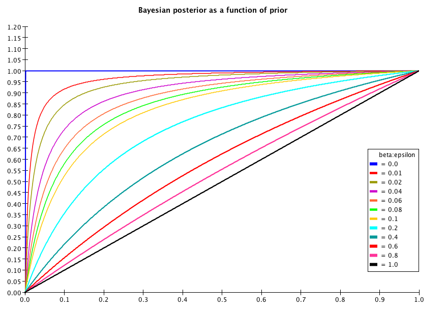
Clearly the posterior probability depends only on the prior probability and on the positive likelihood ratio . Fig. 1 plots for .
Similarly, Eq. (18) asks: when applying the test, which is the conditional posterior probability of being signal ( = true) if the test result is negative ( = false)? Applying Bayes’ theorem to this case yields:
| (24) |
| (25) |
Reverting to the variables of Eqs. (2, 9, 11, 13), Eq. (24) becomes
| (26) |
Similarly to above, the posterior probability depends only on the prior probability and on the negative likelihood ratio .
Calculation of the remaining conditional posterior probabilities and of being background ( = false) if the test result is positive ( = true) or negative ( = false), respectively, is trivial by using Eqs. (19–20).
A priori information are the likelihood ratios and which are obtained from the Monte Carlo simulations, see Section 3. The prior probabilities and are the signal and background fractions, Eq. (2). They are determined by Eq. (4) if the signal to background ratio is known; if not, estimates of them can be calculated from the real data sample by a method presented in Section 6.
5 Event selection
In many experiments, notably those performed by particle collisions, the real data sample has been stochastically accumulated by two independent Poisson processes for signal and background events, respectively.666 In real experiments, the raw data are further affected by triggers of data acquisition, the detector acceptance, reconstruction efficiencies, pre-selection for the analysis proper, etc. These complex aspects, which are beyond the scope of this paper, are discussed e.g. in [5, 6]. Thus, their numbers and behave as random variables with expectation values
| (27) |
where and are fixed values, determined only by the physics laws underlying the production of signal and background events; they are a-priori unknown, but their values can be estimated as shown in section 6.
The base sample thus obtained may be regarded, from a frequentist’s point-of-view, as one stochastic draw from a virtual population, consisting of many repetitions of the experiment at same conditions.
The marginal standard deviations and the correlation 777 The correlation is a characteristic of these distributions, hence it is a constant. It must not be confused with the empirical correlation which is a random variable, dependent on the actual draw, however with expectation value . As can be shown by simulation with an increasing number of draws, plots of the -distribution approach the Dirac function , thus illustrating the fact that is a consistent estimator of . of the bivariate distribution of and are as follows:
| (28) |
Hence, for the total number
| (29) |
However, for dealing with the following selection, is postulated to be a base sample of fixed albeit unknown sizes of (signal) and of (background), and their sum being the fixed and known size of .
A rigorous analysis is deferred to part II of this study.
5.1 Selection procedure
After having determined, with sufficient precision, the characteristic values (8–11) from the Monte Carlo samples and , the same test criteria are now applied on the full real data sample , yielding selected events to enter sub-sample and rejected events to enter sub-sample .
Since and are probabilities of selection and rejection, respectively, and are random variables resulting from two independent Bernoulli processes, with expectation values
| (30) |
| (31) |
Hence with Eq. (14) :
| (32) |
The postulated fixed event numbers “per draw”, and , imply maximal anti-correlation of selected and rejected events,888 A common mistake is tacitly assuming .
| (33) |
and error propagation yields .
5.2 Test optimization
Optimizing the test parameters requires a compromise between minimizing both (loss of genuine signals) and (contamination by genuine background) with regard to the sample of selected events. This can be formalized by defining an appropriate figure of merit (FOM) as a function , thus implicitely affecting the test criteria and , and tuning with the goal of maximizing the FOM fuction .
One might be tempted to base the FOM on real data, e.g. by using the purity , Eq. (51) of Section 7. However, this poses the danger of artificially enhancing a possible statistical fluctuation, hence it must strictly be avoided [7].
6 Estimation of and
The fractions and must be obtained from independent prior knowledge. If the signal to background ratio (SBR) is known, i.e. , their values are determined by Eq. (4), and error propagation yields
| (35) |
Estimates of and are derived straight-forward from Eq. (2).
In the following we assume that SBR is unknown. In this non-trivial case the fractions and are unknown parameters, however, their estimation is possible by using as prior knowledge the test’s characteristic values , applied to the real data sample at hand. The method is described in detail below.
The number of real data events selected and rejected are given by and , respectively, with . These numbers can be used for calculating estimates of the true number of signal and background events, and , respectively, by re-writing Eqs. (30–31) as
| (36) | |||||
| (37) |
or in matrix notation (see Eq. (15)) as
| (38) |
Using Eqs. (14, 16) yields the solutions 999 (see Eq. (16)) ensures non-singularity. The simpler formulae , , as often used instead, are valid only for a negligible contamination rate .
| (39) | |||
| (40) |
obeying . Error propagation, observing (see Eq. (33)), yields the corresponding standard deviations as
| (41) | |||
| (42) |
with given by Eq. (32) and approximately setting and . implies maximal anti-correlation:
| (43) |
and error propagation yields .
Note that the values of Eqs. (41–43) are derived empirically from the observed numbers and . They must not be confused with Eq. (28) which represents characteristics of the distributions determined by the data acquisition.
Estimates of the signal and background fractions, and , are derived straight-forward from Eqs. (39–40) with Eq. (2) as
| (44) |
with , implying maximal anti-correlation:
| (45) |
The estimated values of Eq. (44) can be used as prior probabilities in the Bayesian inference formulae, Eqs. (23, 26) of Section 4. Standard deviations are
| (46) |
7 Data quality
Investigation of the sample , containing selected real events, requires an accurate knowledge of the expected numbers of pure signal events and of contaminating background events within this sample.101010 Such an investigation would typically be summarized like “analysis performed on events, of which are expected to be background”.
Their fractions w.r.t. all selected events, purity 111111 The term “purity” is defined ambigously in the literature. and fraction of contamination, are relevant quantities for judging the data quality:
| (47) |
These fractions and are the probabilities of a selected event to be signal or background, respectively. The number () of signal (background) events within the sample of size is distributed according to the binomial pdf:
| (48) | |||
| (49) |
7.1 Purity
7.2 Fraction of contamination
An estimate of the expected number of background contamination within the selected sample , under the assumption of a non-zero contamination rate, i.e. , can be derived from Eqs. (30, 40), which yields
| (52) |
If knowing the normalization factor , Eq. (5), together with the expected number of wrong positives (simulated background passing the test, see Eq. (10)), above Eq. (52) is equivalent to
| (53) |
with signal to background ratio of real data, Eqs. (3, 39–40)
| (54) |
The fraction of contamination w.r.t. all selected events is
| (55) |
7.3 Zero “wrong positives”
If the test criteria are so tight that no simulated background event survives the test, i.e. implying , then the expectation value , and Eq. (52) and the approximate part of Eq. (53) are no longer valid.
In this case, an estimate of the expectation value follows Bayesian reasoning. Given the sample of simulated background events, and assuming a probability of such an event to pass the test, then the probability of observing events passing this test is given by the binomial pdf
| (56) |
Now we observe events to have passed the test, i.e. . This gives the posterior pdf . Normalization to 1 yields:
| (57) |
with the expectation value
| (58) |
being the probability of a background event to pass the test.
Regarding sample of real background events, Eq. (52) suggests
| (59) |
hence in the sample of real selected events, the expected number of background events is equal to the normalization factor. Inserting into Eq. (53) yields
| (60) |
hence the posterior expectation value of the number of simulated background events wrongly passing the test is one, while their observed number .
Part II: Statistical analysis
8 Assumptions and notation
Let be a data set consisting of recorded events . can be partitioned into the subsets containing the “signal” events and containing the “background” events:
| (61) |
The respective fractions of “signal”and “background” events are denoted by:
| (62) |
A binary indicator is attached to each event i such that
| (63) |
The actual values of the indicators are unknown a priori.
A binary classifier is a function that computes a function value . If , event is classified as “signal”; if , event is classified as “background”. Such a classifier cannot be expected to perform perfectly. The probabilities of correct and wrong decisions can be summarized as follows:
| (64) |
where is the probability of classifying a “signal” event as being “background” (type I error), and is the probability of classifying a “background” event as being “signal” (type II error). It is required that , see Eq. (16). The difference will be denoted by .
The probabilities and are unknown a priori, but can be estimated to arbitrary precision from an independent, sufficiently large simulated sample , for which the classification of events into “signal”and “background” is known, see Section 3. In the following, and will be considered as known constants.
The respective probabilities of classifying an arbitrary event as “signal” or “background” are given by:
| (65) |
The respective numbers and of events classified by as “signal” and “background” are given by:
| (66) |
9 Bayesian estimation
Conditional on , is distributed according to the binomial distribution Bino() with the probability function:
| (67) |
The posterior pdf of , given an observation , can be written down in closed form if the prior pdf is taken from the conjugate family of priors, which is the Beta family in this case [9].
If the prior distribution of is Beta(), the posterior pdf is given by:
| (68) |
The Bayes estimator, i.e., the posterior mean and its variance are equal to:
| (69) |
where is the expectation of the random variable and is its variance.
If no prior information on is available, there are three popular “uninformative” priors 121212 The maximum-entropy prior and Jeffrey’s prior are not really uninformative, as they assign a specific probability to any interval that is contained in , see [10]. Neither is Haldane’s improper prior, as it can be considered as the limit of Beta() for , thus in the limit assigning the probability of 0.5 to both and . in the unit interval:
-
1.
the maximum-entropy prior Beta()=Unif(): ;
-
2.
Jeffrey’s prior Beta(): ;
-
3.
Haldane’s improper prior Beta(): .
Prior knowledge about can be incorporated via an informative prior. For example, assume that it is known that is about 0.4, with a standard uncertainty of about 0.1. This information can be encoded by a Beta prior Beta() with mean 0.4 and variance 0.01:
| (70) |
Credible intervals for can be computed via quantiles of the posterior distribution. A symmetric credible interval with probability content of is given by , where is the -quantile of the posterior pdf in Eq. 68 and is the -quantile.
An HPD interval can be computed by solving the following system of non-linear equations:
| (71) | ||||
| (72) |
where is the posterior pdf in Eq. 68 and is its cumulative distribution function. A MATLAB code snippet that solves the system is shown in Fig. 2.
9.1 Transformation to and
Solving Eq. (65) for yields:
| (73) |
As this is an affine transformation, the posterior mean and variance of and are given by:
| (74) | |||
| (75) |
The bounds of credible and HPD intervals are transformed in the same way.
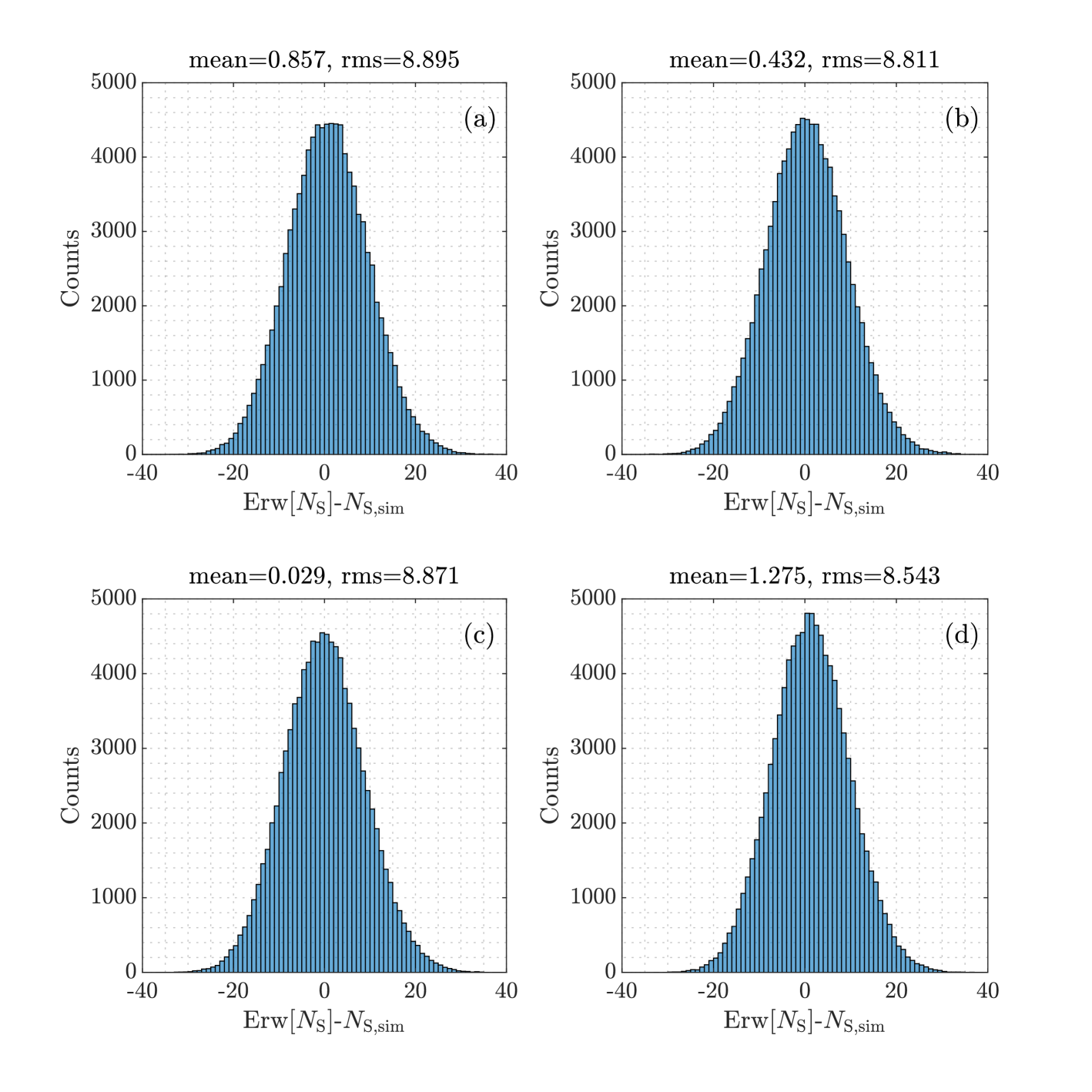
Example 1
Assume . Then Figure 3 shows histograms of the difference in simulated samples, with three non-informative priors and an informative prior. The informative prior Beta() in subplot (d) encodes the prior information with a standard uncertainty of 0.05 (). The estimates in (d) have the largest bias, but the smallest rms error.
10 Frequentist estimation
From a frequentist point of view, the observed data set is drawn at random from a (virtual or fictitious) parent population that has to be specified by the person(s) performing the data analysis. From now on, is a random variable that denotes the size of the elements of the population; the quantities are random variables, too. In contrast to the Bayesian viewpoint, the fraction of “signal” events is an unknown fixed parameters to be estimated. Of course it is assumed that all data sets in the parent population have the same average fraction of “signal” events. The size of the observed data set is denoted by the constant .
The specification of the parent population is neither unique nor always obvious, and each choice will lead to a different assessment of the unconditional moments of the estimates and . However, conditional on the observed size of the data set, the moments are always the same. This point is illustrated by three choices of parent populations, the first one with fixed (Subsection 10.1), the second one with Poisson-distributed (Subsection 10.2), the third one with drawn from a mixture of Poisson distributions (Subsection 10.3).
10.1 Data set size is fixed
If is fixed, the unconditional distribution of is the same as the conditional distribution, i.e., Bino(), and the distribution of is Bino(), with . It follows that:
| (76) | |||
| (77) |
where cov(X,Y) is the covariance of and and is their correlation. It follows that:
| (78) | |||
| (79) |
The relation between and can be written in the following way (see Eq. (65)):
| (80) |
Using Eq. (80), it is easy to show that
| (81) |
is an unbiased estimator of :
| (82) |
The joint variance-covariance matrix of can be computed from Eq. (81) by linear error propagation:
| (83) |
The relative frequencies and are estimated by:
| (84) |
These estimators are unbiased, and their expectation and variance-covariance matrix is equal to:
| (85) | ||||
| (86) | ||||
| (87) |
can also be written as:
| (88) |
Conditional on , the observable is the sum of two random variables and , where () is the number of signal (background) events classified as “signal”. The distribution of is therefore Bino(), and the distribution of is Bino(). It follows that:
| (89) | |||
| (90) | |||
| (91) |
Still conditional on , we have:
| (92) | |||
| (93) | |||
| (94) |
and are correlated. From Eq. (89) follows:
| (95) |
As , we finally obtain:
| (96) | ||||
| (97) |
It follows from Eq. (96) that and are uncorrelated:
| (98) |
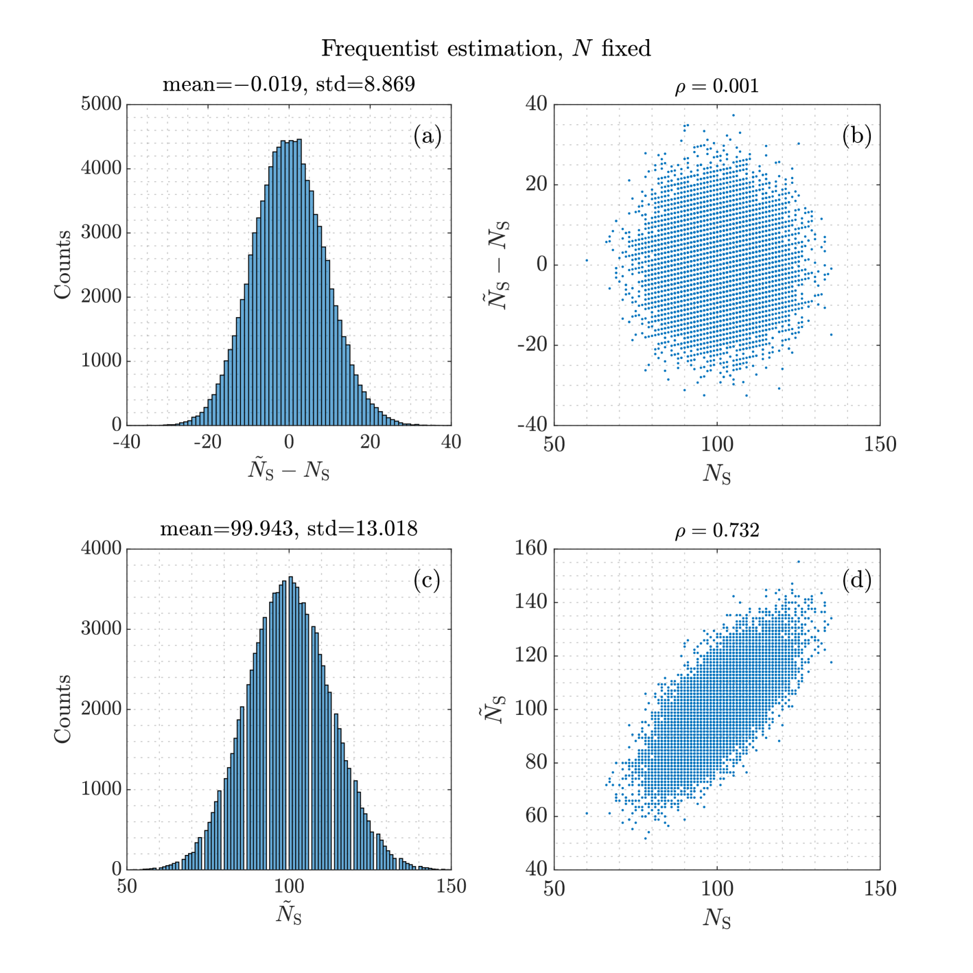
Example 2
Using the numerical values of Example 1, Table 1 shows the expectations, the standard deviations and the correlation of averaged over a simulated population with data sets. The exact values are shown as well. Figure Fig. 4 shows histograms and scatter plots of the estimates and .
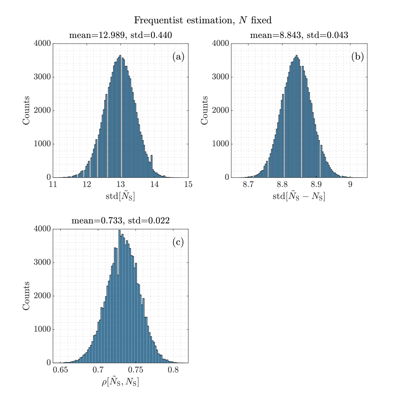
The variances and covariances derived in this subsection ultimately depend on the unknown parameter . In practice, has to be replaced by its estimated value, leading to a deviation from the exact theoretical value. The size of the deviations is illustrated in Fig. 5, which shows histograms of , and . The entries are the approximative standard deviations that use and instead of and .
10.2 Data set size is Poisson-distributed
Next it is assumed that
-
•
each data set in the population is the union of a set of size and a set of size ;
-
•
and are independent Poisson-distributed random variables with mean values and , respectively.
The data set size ist then Poisson distributed according to Pois(). In the absence of further external information, the obvious choice of the Poisson parameter is .
Conditional on , we have:
| (99) | |||
| (100) | |||
| (101) |
If are estimated via Eq. (81), their conditional expectation and variance-covariance matrix is given by:
| (102) | ||||
| (103) | ||||
| (104) |
The unknown fractions are estimated by:
| (105) |
Conditional on , these estimators are unbiased. Their expectation and conditional variance-covariance matrix is equal to:
| (106) | ||||
| (107) | ||||
| (108) |
The unconditional expectations and elements of the variance-covariance matrix can be calculated by taking the expectation with respect to the distribution of , which is Pois(). First, the conditional second moments around 0 (i.e., raw moments) are computed:
| (109) | |||
| (110) | |||
| (111) |
Taking the expectation of over Pois() yields:
| (112) | |||
| (113) | |||
| (114) | |||
| (115) |
The unconditional variance-covariance matrix is then given by:
| (116) | |||
| (117) | |||
| (118) | |||
| (119) |
Example 3
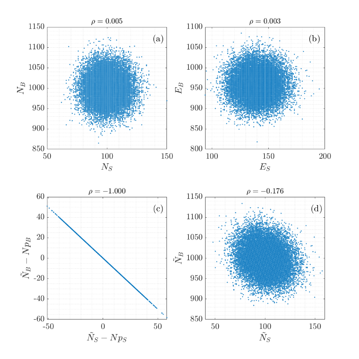
Using the numerical values of Example 1, the exact conditional expectations, standard deviations and correlation of are identical to the ones shown in Table 1. Table 2 shows the corresponding unconditional values with . Fig. 6 shows scatter plots of versus , versus , versus , and versus .
10.3 Data set size is drawn from a mixture
of Poisson distributions
An even more general parent distribution is obtained by assuming that the size of the data sets in the population is distributed according to a mixture of Poisson distributions. This means that the data set size is drawn from a Poisson distribution with mean , and is drawn from a mixing distribution with mean and variance . The results of the previous subsection show that conditional on :
| (120) |
This yields the following second raw moments:
| (121) |
The computation of the unconditional moments relies on the fact that the raw moments of a mixture are a mixture of the raw moments of the mixture components. It follows that:
| (122) | |||
where denotes the expectation with respect to the mixing distribution . The final step is the computation of the full unconditional variance-covariance matrix of :
| (123) | |||
Using Eq. (81) and linear error propagation, , their expectations and their joint variance-covariance matrix can be computed, see Subsection 3.2. The explicit formulas are too complicated to be spelled out here. Note that two mixing distributions with the same mean and variance give the same estimates.
The special case where is a Poisson distribution is of particular interest. As in this case, the following variance-covariance matrix of is obtained:
| (124) |
Linear error propagation gives the following joint variance-covariance matrix of :
| (125) | |||
| (126) |
In the absence of further external information, the obvious choice of the Poisson parameter is .
11 Discussion
Conditional on the data set size , the distribution of the estimates is always the same. The conditional estimates are identical to the Bayes estimate with Haldane’s prior, their conditional variance is, however, slightly different from the posterior variance of the Bayes estimator. The unconditional moments of depend of course on the assumptions about the parent population, so different data analysts may come to different conclusions. In addition, if only a single data set has been observed, the conditional moments are much more meaningful.
An advantage of the Bayesian approach is that prior information about the “signal” content of the data set can be easily incorporated into the Bayes estimator by a conjugate Beta prior. On the other hand, with the exception of Haldane’s prior, the Bayes estimators have a small bias when compared to the “truth” value used in the simulation, and different data analysts may prefer different priors, whether uninformative or informative.
References
-
[1]
F. James:
Statistical Methods in Experimental Physics, ed.
World Scientific, Singapore 2006 (ISBN 981-270-527-9). -
[2]
L. Lyons:
Statistics for Nuclear and Particle Physicists,
Cambridge University Press, 1992 (ISBN 0-521-37934-2). -
[3]
D.S. Sivia:
Data Analysis – A Bayesian Tutorial, ed.
Oxford University Press, 2008 (ISBN 978-0-19-856832-2). -
[4]
G. D’Agostini:
Bayesian Reasoning in High-Energy Physics,
Yellow Report CERN 99-03, Geneva 1999. -
[5]
R. Frühwirth, M. Regler, R.K. Bock, H. Grote, D. Notz:
Data Analysis Techniques for High-Energy Physics, ed.
Cambridge University Press, 2000 (ISBN 0-521-63548-9). -
[6]
C.W. Fabjan and H. Schopper (editors):
Particle Physics Reference Library, vol. 2.
Springer Open, Berlin 2020 (DOI: 10.1007/978-3-030-35318-6). -
[7]
F. Porter (editor):
The Physics of the B Factories, chapter 4,
Eur.Phys.J. C 74 (2014) 3026, pp. 59–66, and
Springer Open, Berlin 2014 (arXiv:1406.6311 [hep-ex]). -
[8]
P. Feichtinger et al.:
Punzi-loss,
Eur.Phys.J. C 82 (2022) 121 (arXiv:2110.00810 [hep-ex]). -
[9]
J.M. Bernardo and A.F.M. Smith:
Bayesian Theory.
John Wiley&Sons, Hoboken NJ, 1994 (ISBN 0-471-92416-4). -
[10]
P.B. Stark:
Constraints versus Priors,
SIAM/ASA J. Uncertainty Quantification 3 (2015) 586
(DOI: 10.1137/130920721).