mkchung@wisc.edu
Statistical Analysis on Brain Surfaces
Abstract
In this paper, we review widely used statistical analysis frameworks for data defined along cortical and subcortical surfaces that have been developed in last two decades. The cerebral cortex has the topology of a 2D highly convoluted sheet. For data obtained along curved non-Euclidean surfaces, traditional statistical analysis and smoothing techniques based on the Euclidean metric structure are inefficient. To increase the signal-to-noise ratio (SNR) and to boost the sensitivity of the analysis, it is necessary to smooth out noisy surface data. However, this requires smoothing data on curved cortical manifolds and assigning smoothing weights based on the geodesic distance along the surface. Thus, many cortical surface data analysis frameworks are differential geometric in nature (Chung, 2012). The smoothed surface data is then treated as smooth random fields and statistical inferences can be performed within Keith Worsley’s random field theory (Worsley et al., 1996, 1999). The methods described in this paper are illustrated with the hippocampus surface data set published in (Chung et al., 2011). Using this case study, we will determine if there is an effect of family income on the growth of hippocampus in children in detail. There are a total of 124 children and 82 of them have repeat magnetic resonance images (MRI) two years later.
1 Introduction
The cerebral cortex has the topology of a 2D convoluted sheet. Most of the features that distinguish these cortical regions can only be measured relative to the local orientation of the cortical surface (Dale & Fischl, 1999). As the brain develops over time, cortical surface area expands and its curvature changes (Chung, 2012). It is equally likely that such age-related changes with respect to the cortical surface are not uniform (Chung et al., 2003; Thompson et al., 2000). By measuring how geometric features such as the cortical thickness, curvature and local surface area change over time, statistically significant brain tissue growth or loss in the cortex can be detected locally at the vertex level.
The first obstacle in performing surface-based data analysis is a need for extracting cortical surfaces from MRI volumes. This requires correcting MRI field inhomogeneity artifacts. The most widely used technique is the nonparametric nonuniform intensity normalization method (N3) developed at the Montreal neurological institute (MNI), which eliminates the dependence of the field estimate on anatomy (Sled et al., 1988). The next step is the tissue classification into three types: gray matter, white matter and cerebrospinal fluid (CSF). This is critical for identifying the tissue boundaries where surface measurements are obtained. An artificial neural network classifier (Kollakian, 1996; Ozkan et al., 1993) or Gaussian mixture models (Good et al., 2001) can be used to segment the tissue types automatically. The Statistical Parametric Mapping (SPM) package111The SPM package is available at www.fil.ion.ucl.ac.uk/spm. uses a Gaussian mixture with a prior tissue density map.
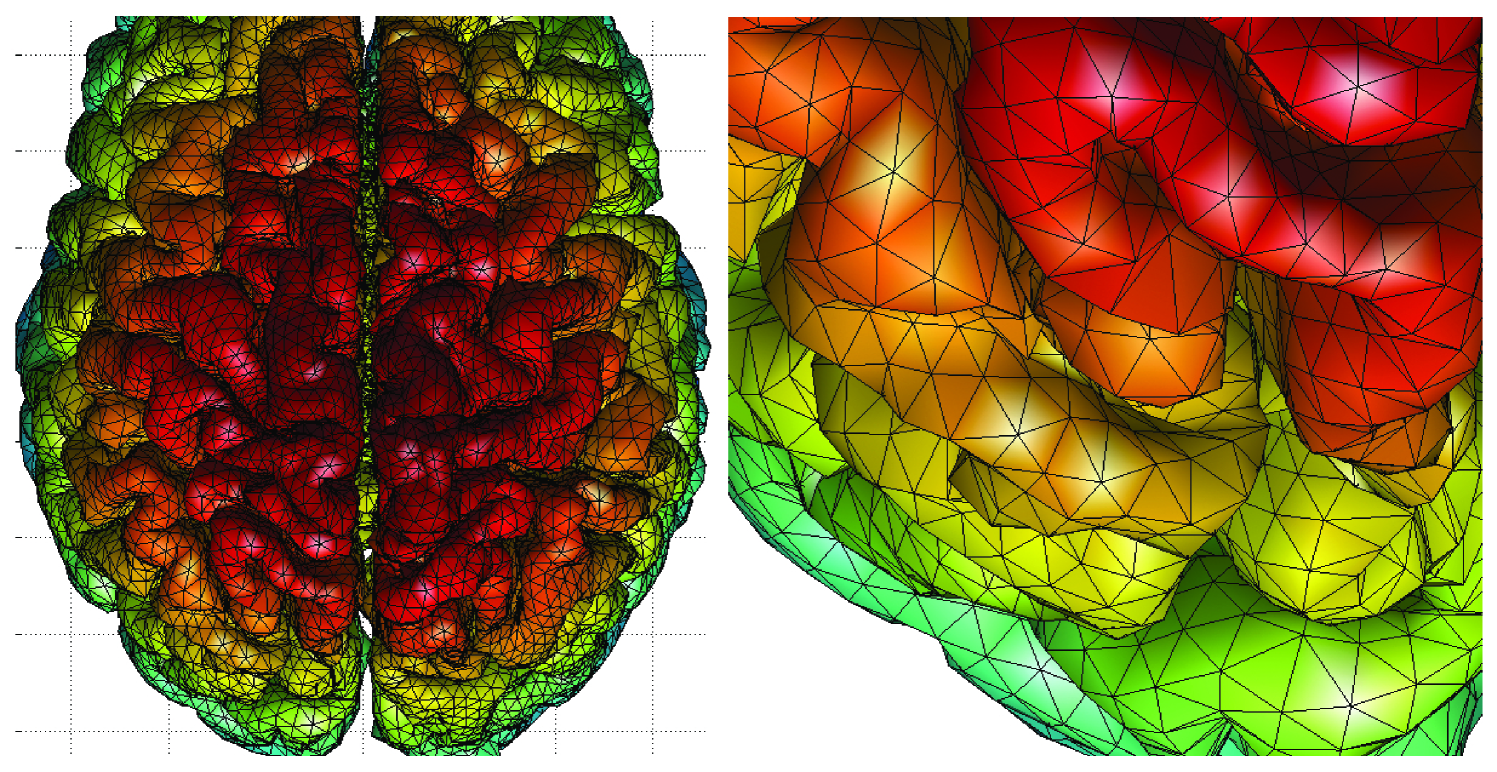
After the segmentation, the tissue boundaries are extracted as triangular meshes. In order to triangulate the boundaries, the marching cubes algorithm (Lorensen & Cline, 1987), level set method (Sethian, 2002), the deformable surfaces method (Davatzikos & Bryan, 1995) or anatomic segmentation using proximities (ASP) method (MacDonald et al., 2000) can be used. Brain substructures such as the brain stem and the cerebellum are usually automatically removed in the process. The resulting triangular mesh is expected to be topologically equivalent to a sphere. For example, the triangular mesh resulted from the ASP method consists of 40,962 vertices and 81,920 triangles with the average internodal distance of . Figure 1 shows a representative cortical mesh obtained from ASP. Surface measurements such as cortical thickness can be automatically obtained at each mesh vertex. Subcortical brain surfaces such as amygdala and hippocampus are extracted similarly, but often done in a semi-automatic fashion with the marching cubes algorithm on manual edited subcortical volumes. In the hippocampus case study, the left and right hippocampi were manually segmented in the template using the protocol outlined in (Rusch et al., 2001).
Comparing measurements defined across different cortical surfaces is not trivial due to the fact that no two cortical surfaces are identically shaped. In comparing measurements across different 3D whole brain images, 3D volume-based image registration such as Advanced Normalization Tools (ANTS) (Avants et al., 2008) is needed. However, 3D image registration techniques tend to misalign sulcal and gyral folding patterns of the cortex. Hence, 2D surface-based registration is needed in order to match measurements across different cortical surfaces. Various surface registration methods have been proposed (Chung et al., 2005; Chung, 2012; Thompson & Toga, 1996; Davatzikos, 1997; Miller et al., 1997; Fischl et al., 1999). Most methods solve a complicated optimization problem of minimizing the measure of discrepancy between two surfaces. A much simpler spherical harmonic representation technique provide a simple way of approximately matching surfaces without time-consuming numerical optimization (Chung, 2012).
Surface registration and the subsequent surface-based analysis usually require parameterizing surfaces. It is natural to assume the surface mesh to be a discrete approximation to the underlying cortical surface, which can be treated as a smooth 2D Riemannian manifold. Cortical surface parameterization has been done previously in (Thompson & Toga, 1996; Joshi et al., 1995; Chung, 2012). The surface parameterization also provides surface shape features such as the Gaussian and mean curvatures, which measure anatomical variations associated with the deformation of the cortical surface during, for instance, development and aging (Dale & Fischl, 1999; Griffin, 1994; Joshi et al., 1995; Chung, 2012).
2 Surface Parameterization
In order to perform statistical analysis on a surface, parameterization of the surface is often required (Chung, 2012). Brain surfaces are often mapped onto a plane or a sphere. Then surface measurements defined on mesh vertices are also mapped onto the new domain and analyzed. However, almost all surface parameterizations suffer metric distortions, which in turn influence the spatial covariance structure so it is not necessarily the best approach.
We model the cortical surface as a smooth 2D Riemannian manifold parameterized by two parameters and such that any point can be represented as
for some parameter space (Boothby, 1986; do Carmo, 1992; Chung et al., 2003; Kreyszig, 1959). The aim of the parameterization is estimating the coordinate functions as smoothly as possible.
Both global and local parameterizations are available. A global parameterization, such as tensor B-splines and spherical harmonic representation, are computationally expensive compared to a local surface parameterization. A local surface parameterization in the neighborhood of point can be obtained via the projection of the local surface patch onto the tangent plane (Chung, 2012; Joshi et al., 1995).
2.1 Local Parameterization by Quadratic Polynomial
A local parameterization is usually done by fitting a quadratic polynomial of the form
| (1) |
in . The data can be centered so there is no constant term in the quadratic form (1) (Chung, 2012). The coefficients are usually estimated by the least squares method (Joshi et al., 1995; Khaneja et al., 1998; Chung, 2012).
In estimating various differential geometric measures such as the Laplace-Beltrami operator or curvatures, it is not necessary to find global surface parameterization of . Local surface parameterization such as the quadratic polynomial fit is sufficient to obtain such geometric quantities (Chung, 2012). The drawback of the polynomial parameterization is that there is a tendency to weave the outermost mesh vertices to find vertices in the center. Therefore this is not advisable to directly fit (1) when one of the coordinate values rapidly changes.
2.2 Surface Flattening
Parameterizing cortical and subcortical surfaces with respect to simpler algebraic surfaces such as a unit sphere is needed to establish a standard coordinate system. However, polynomial regression type of local parameterization is ill-suited for this purpose. For the global surface parameterization, we can use surface flattening (Andrade et al., 2001; Angenent et al., 1999), which is nonparametric in nature. The surface flattening parametrizes a surface by either solving a partial differential equation or optimizing its variational form.
Deformable surface algorithms naturally provide one-to-one maps from cortical surfaces to a sphere since the algorithm initially starts with a spherical mesh and deforms it to match the tissue boundaries (MacDonald et al., 2000). The deformable surface algorithms usually start with the second level of triangular subdivision of an icosahedron as the initial surface. After several iterations of deformation and triangular subdivision, the resulting cortical surface contains very dense triangle elements. There are many surface flattening techniques such as conformal mapping (Angenent et al., 1999; Gu et al., 2004; Hurdal & Stephenson, 2004) quasi-isometric mapping (Timsari & Leahy, 2000), area preserving mapping (Brechbuhler et al., 1995), and the Laplace equation method (Chung, 2012).
For many surface flattening methods to work, the starting binary object has to be close to star-shape or convex. For shapes with a more complex structure, the methods may create numerical singularities in mapping to the sphere. Surface flattening can destroy the inherent geometrical structure of the cortical surface due to the metric distortion. Any structural or functional analysis associated with the cortex can be performed without surface flattening if the intrinsic geometric method is used (Chung, 2012).
2.3 Spherical Harmonic Representation
The spherical harmonic (SPHARM) representation
222The SPHARM package is available at
www.stat.wisc.edu/mchung/softwares/weighted-SPHARM/weighted-SPHARM.html
is a widely used subcortical surface parameterization technique (Chung et al., 2008; Chung, 2012; Gerig et al., 2001; Gu et al., 2004; Kelemen et al., 1999; Shen et al., 2004). SPHARM represents the coordinates of mesh vertices as a linear combination of spherical harmonics. SPHARM has been mainly used as a data reduction technique for compressing global shape features into a small number of coefficients. The main global geometric features are encoded in low degree coefficients while the noise are in high degree spherical harmonics (Gu et al., 2004). The method has been used to model various subcortical structures such as ventricles (Gerig et al., 2001), hippocampi (Shen et al., 2004) and cortical surfaces (Chung et al., 2008). The spherical harmonics have a global support. So the resulting spherical harmonic coefficients contain the global shape features and it is not possible to directly obtain local shape information from the coefficients only. However, it is still possible to obtain local shape information by evaluating the representation at each fixed vertex, which gives the smoothed version of the coordinates of surfaces. In this fashion, SPHARM can be viewed as mesh smoothing (Chung et al., 2008, n.d.). In this section, we present a brief introduction of SPHARM within a Hilbert space framework.
Suppose there is a bijective mapping between the cortical surface and a unit sphere obtained through a deformable surface algorithm (Chung, 2012). Consider the parameterization of by
with . The polar angle is the angle from the north pole and the azimuthal angle is the angle along the horizontal cross-section. Using the bijective mapping, we can parameterize functional data with respect to the spherical coordinates
| (2) |
where is a unknown smooth coordinate function and is a zero mean random field, possibly Gaussian. The error function accounts for possible mapping errors. The unknown signal is then estimated in the finite subspace of , the space of square integrable functions in , spanned by spherical harmonics in the least squares fashion (Chung et al., 2008).
Previous imaging and shape modeling literature have used the complex-valued spherical harmonics (Bulow, 2004; Gerig et al., 2001; Gu et al., 2004; Shen et al., 2004). In practice, however, it is sufficient to use only real-valued spherical harmonics (Courant & Hilbert, 1953; Homeier & Steinborn, 1996), which is more convenient in setting up a real-valued stochastic model (2). The relationship between the real- and complex-valued spherical harmonics is given in (Blanco et al., 1997; Homeier & Steinborn, 1996). The complex-valued spherical harmonics can be transformed into real-valued spherical harmonics using an unitary transform.
The spherical harmonic of degree and order is defined as
where and is the associated Legendre polynomial of order (Courant & Hilbert, 1953; Wahba, 1990), which is given by
The first few terms of the spherical harmonics are
The spherical harmonics are orthonormal with respect to the inner product
where and the Lebesgue measure . The norm is then defined as
| (3) |
The unknown mean function is estimated by minimizing the integral of the squared residual in , the space spanned by up to -th degree spherical harmonics:
| (4) |
It can be shown that the minimization is given by
| (5) |
the Fourier series expansion. The expansion (5) has been referred to as the spherical harmonic representation (Chung et al., 2008; Gerig et al., 2001; Gu et al., 2004; Shen et al., 2004; Shen & Chung, 2006). This technique has been used in representing various brain subcortical structures such as hippocampi Shen et al. (2004) and ventricles (Gerig et al., 2001) as well as the whole brain cortical surfaces (Chung et al., 2008; Gu et al., 2004). By taking each component of Cartesian coordinates of mesh vertices as the functional signal , surface meshes can be parameterized as a function of and .
The spherical harmonic coefficients can be estimated in least squares fashion. However, for an extremely large number of vertices and expansions, the least squares method may be difficult to directly invert large matrices. Instead, the iterative residual fitting (IRF) algorithm (Chung et al., 2008) can be used to iteratively estimate the coefficients by partitioning the larger problem into smaller subproblems. The IRF algorithm is similar to the matching pursuit method (Mallat & Zhang, 1993). The IRF algorithm was developed to avoid the computational burden of inverting a large linear problem while the matching pursuit method was originally developed to compactly decompose a time-frequency signal into a linear combination of a pre-selected pool of basis functions. Although increasing the degree of the representation increases the goodness-of-fit, it also increases the number of estimated coefficients quadratically. So it is necessary to stop the iteration at the specific degree , where the goodness-of-fit and the number of coefficients balance out. This idea was used in determining the optimal degree of SPHARM (Chung et al., 2008).
The limitation of SPHARM is that it produces the Gibbs phenomenon, i.e., ringing artifacts, for discontinuous and rapidly changing continuous measurements (Chung et al., 2008; Gelb, 1997). The Gibbs phenomenon can be effectively removed by weighting the spherical harmonic coefficients exponentially smaller, which makes the representation smooth out rapidly changing signals. The weighted version of SPHARM is related to isotropic diffusion smoothing (Andrade et al., 2001; Cachia, Mangin, Riviére, Kherif, Boddaert, Andrade, Papadopoulos-Orfanos, Poline, Bloch, Zilbovicius, Sonigo, Brunelle & Régis, 2003; Chung, 2012; Chung et al., 2005) as well as the diffusion wavelet transform (Chung et al., 2008, n.d.; Hosseinbor et al., 2014).
3 Surface Registration
To construct a test statistic locally at each vertex across different surfaces, one must register the surfaces to a common template surface. Nonlinear cortical surface registration is often performed by minimizing objective functions that measure the global fit of two surfaces while maximizing the smoothness of the deformation in such a way that the cortical gyral or sulcal patterns are matched smoothly (Chung et al., 2005; Robbins, 2003; Thompson & Toga, 1996). There is also a much simpler way of aligning surfaces using SPHARM representation (Chung et al., 2008). Before any sort of nonlinear registration is performed, an affine registration is performed to align and orient the global brain shapes.
3.1 Affine Registration
Anatomical objects extracted from 3D medical images are aligned using affine transformations to remove the global size differences. Affine registration requires identifying corresponding landmarks either manually or automatically. The affine transform of point to is given by
where the matrix corresponds to rotation, scaling and shear while corresponds to translation. Although the affine transform is not linear, it can be made into a linear form by augmenting the transform. The affine transform can be rewritten as
| (12) |
Let
Trivially, is linear a linear operator. The matrix is the most often used form for recording the affine registration.
Let be the -th landmark and its corresponding affine transformed points . Then we rewrite (12) as
Then the least squares estimation is given as
Then the points are mapped to , which may not coincide with in general. In practice, landmarks are automatically identified from T1-weighted MRI.
3.2 SPHARM Correspondence
Using SPHARM, it is possible to approximately register surfaces with different mesh topology without any optimization. The crude alignment can be done by coinciding the first order ellipsoid meridian and equator in the SPHARM representation (Gerig et al., 2001; Styner et al., 2006). However, this can be improved. Consider SPHARM representation of surface with spherical angles given by
where are the coordinates of mesh vertices and SPHARM coefficient . Consider another SPHARM representation obtained from mesh coordinate :
where . Suppose the surface is deformed to by the amount of displacement . We wish to find that minimizes the discrepancy between and in the subspace spanned using up to the -th degree spherical harmonics. It can be shown that
| (14) |
This implies that the optimal displacement of matching two surfaces is obtained by simply taking the difference between two SPHARM and matching coefficients of the same degree and order. Then a specific point in one surface corresponds to in the other surface. We refer to this point-to-point surface matching as the SPHARM correspondence (Chung et al., 2008). Unlike other surface registration methods (Chung et al., 2005; Robbins, 2003; Thompson & Toga, 1996), it is not necessary to consider an additional cost function that guarantees the smoothness of the displacement field since the displacement field is already a linear combination of smooth basis functions.
3.3 Diffeomorphic Registration
Diffeomorphic image registration is a recently popular technique for registering volume and surface data (Avants et al., 2008; Miller & Qiu, 2009; Vaillant et al., 2007; Qiu & Miller, 2008; Yang et al., 2011). From the affine transformed individual surfaces , an additional nonlinear surface registration to the template using the large deformation diffeomorphic metric mapping (LDDMM) framework can be performed (Miller & Qiu, 2009; Vaillant et al., 2007; Qiu & Miller, 2008; Yang et al., 2011). In LDDMM, given the template surface , the diffeomorphic transformations, which are one-to-one, smooth forward, and inverse transformation, are constructed as follows. We estimate the diffeomorphism between them as a smooth streamline given by the Lagrangian evolution:
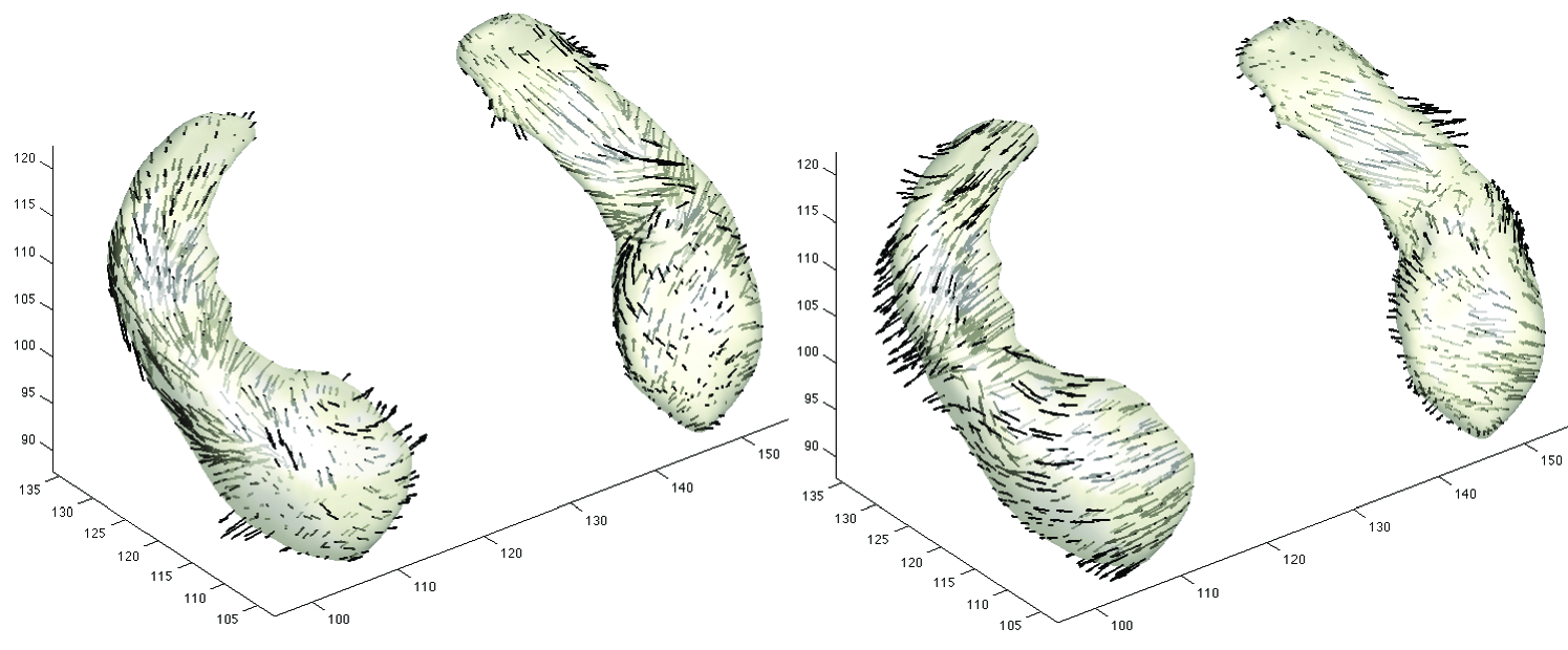
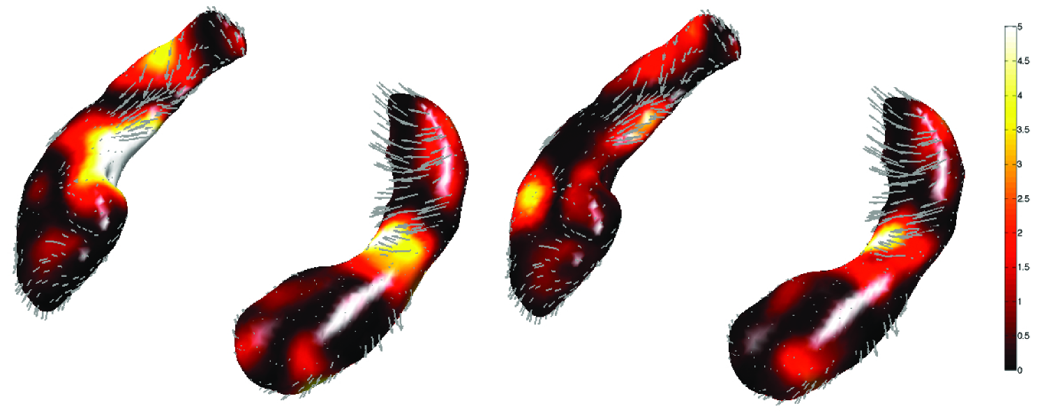
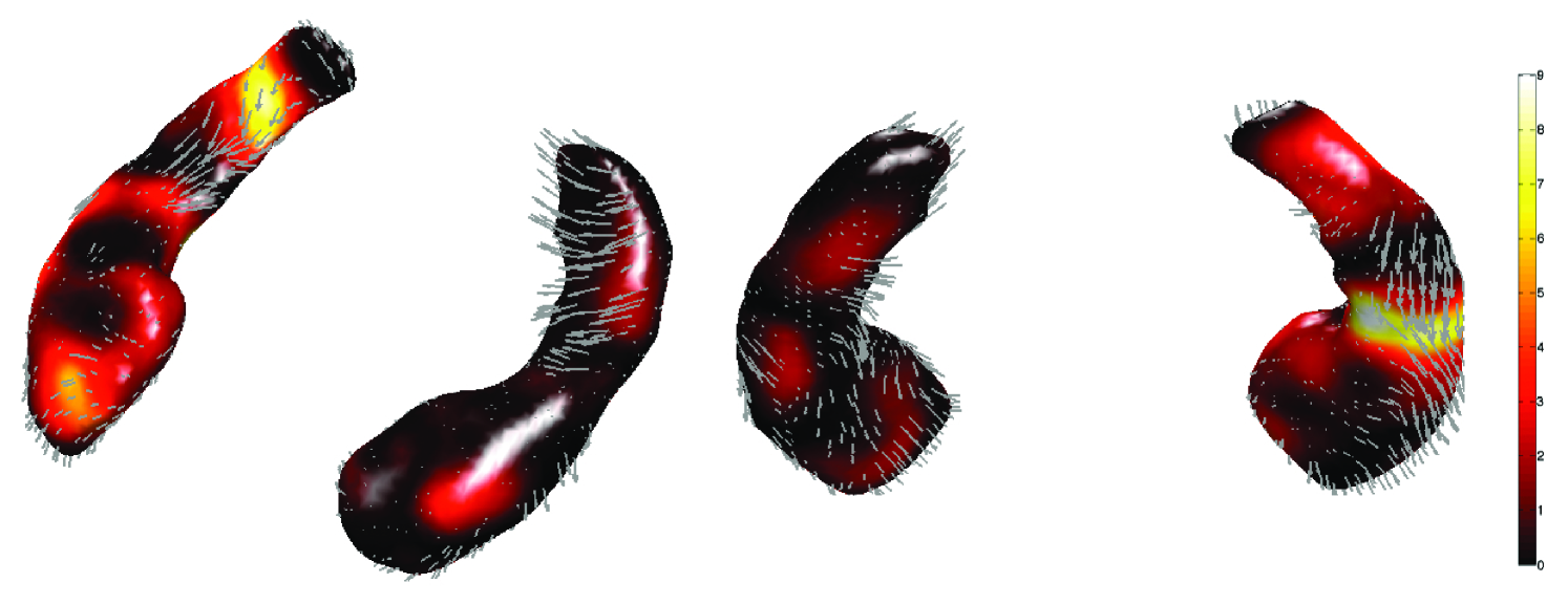
with for time-dependent velocity field . Note the surfaces and are the start and end points of the diffeomorphism, i.e. and . By solving the evolution equation numerically, we obtain the diffeomorphism. By averaging the inverse deformation fields from the template to individual subjects, we may obtain yet another final more refined template. The vector fields are constrained to be sufficiently smooth to generate diffeomorphic transformations over finite time (Dupuis et al., 1998). Figure 2 shows the resulting displacement vector fields of warping from the template to two hippocampal surfaces. In the deformation-based morphometry, variability in the displacement is used to characterize surface growth and differences (Chung, 2012).
4 Cortical Surface Features
The human cerebral cortex has the topology of a 2D highly convoluted grey matter shell with an average thickness of 3 mm (Chung, 2012; MacDonald et al., 2000). The outer boundary of the shell is called the outer cortical surface while the inner boundary is called the inner cortical surface. Various cortical surface features such as curvatures, local surface area and cortical thickness have been used in quantifying anatomical variations. Among them, cortical thickness has been more often analyzed than other features.
4.1 Cortical Thickness
Once we extract both the outer and inner cortical surface meshes, cortical thickness can be computed at each mesh vertex. The cortical thickness is defined as the distance between the corresponding vertices between the inner and outer surfaces (MacDonald et al., 2000). There are many different computational approaches in measuring cortical thickness. In one approach, the vertices on the inner triangular mesh are deformed to fit the outer surface by minimizing a cost function that involves bending, stretch and other topological constraints (Chung, 2012). There is also an alternate method for automatically measuring cortical thickness based on the Laplace equation (Jones et al., 2000).
The average cortical thickness for each individual is about 3 mm (Henery & Mayhew, 1989). Cortical thickness varies from 1 to 4 mm depending on the location of the cortex. In normal brain development, it is highly likely that the change of cortical thickness may not be uniform across the cortex. Since different clinical populations are expected to show different patterns of cortical thickness variations, cortical thickness has also been used as a quantitative index for characterizing a clinical population (Chung et al., 2005). Cortical thickness varies locally by region and is likely to be influenced by aging, development and disease (Barta et al., 2005). By analyzing how cortical thickness varies between clinical and non-clinical populations, we can locate regions on the brain related to a specific pathology.
4.2 Surface Area and Curvatures
As in the case of local volume changes in the deformation-based morphometry, the rate of cortical surface area expansion or reduction may not be uniform across the cortical surface (Chung, 2012). Suppose that cortical surface is parameterized by the parameters such that any point can be written as . Let be the partial derivative vectors. The Riemannian metric tensor is then given by the inner product between two vectors and , i.e.
The tensor measures the amount of the deviation of the cortical surface from a flat Euclidean plane and can be used to measure lengths, angles and areas on the cortical surface.
Let be a matrix of metric tensors. The total surface area of the cortex is then given by
where is the parameter space (Kreyszig, 1959). The term is called the surface area element and it measures the transformed area of the unit square in the parameter space via transformation . The surface area element can be considered as the generalization of the Jacobian determinant, which is used in measuring local volume changes in the tensor-based morphometry (Chung, 2012).
Instead of using the metric tensor formulation, it is possible to quantify local surface area change in terms of the areas of the corresponding triangles in surface meshes. However, this formulation assigns the computed surface area to each face instead of each vertex. This causes a problem in both surface-based smoothing and statistical analysis, where values are required to be given on vertices. Interpolating scalar values on vertices from face values can be done by the weighted average of face values. It is not hard to develop surface-based smoothing and statistical analysis on face values, as a form of dual formulation, but the cortical thickness and the curvature metric are defined on vertices so we end up with two separate approaches: one for metrics defined on vertices and the other for metrics defined on faces. Therefore, the metric tensor approach provides a better unified quantitative framework for the subsequent statistical analysis.
The principal curvatures characterize the shape and location of the sulci and gyri, which are the valleys and crests of the cortical surfaces (Bartesaghi & Sapiro, 2001; Joshi et al., 1995; Khaneja et al., 1998). By measuring the curvature changes, rapidly folding and cortical regions can be localized. The principal curvatures and can be represented as functions of in quadratic surface (1) (Boothby, 1986; Kreyszig, 1959).
4.3 Gray Matter Volume
Local volume can be computed using the determinant of the Jacobian of deformation and used in detecting the regions of brain tissue growth and loss in brain development (Chung, 2012). Compared to the local surface area change, the local volume change measurement is more sensitive to small deformation of the brain. If a unit cube increases its sides by one, the surface area will increase by while the volume will increase by . Therefore, the statistical analysis based on the local volume change is at least twice more sensitive compared to that of the local surface area change. So the local volume change should be able to pick out gray matter tissue growth patterns even when the local surface area change may not.
The gray matter can be considered as a thin shell bounded by two surfaces with varying cortical thickness. In most deformable surface algorithms like FreeSurfer, each triangle on the outer surface has a corresponding triangle on the inner surface. Let be the three vertices of a triangle on the outer surface and be the corresponding three vertices on the inner surface such that is linked to . Then the volume of the triangular prism is given by the sum of the determinants
where
is the volume of a tetrahedron whose vertices are . Afterwards, the total gray matter volume can be estimated by summing the volumes of all triangular prisms (Chung, 2012).
5 Surface Data Smoothing
Cortical surface mesh extraction and cortical thickness computation are expected to introduce noise (Chung et al., 2005; Fischl & Dale, 2000; MacDonald et al., 2000). To counteract this, surface-based data smoothing is necessary (Andrade et al., 2001; Cachia, Mangin, Riviére, Papadopoulos-Orfanos, Kherif, Bloch & Régis, 2003; Cachia, Mangin, Riviére, Kherif, Boddaert, Andrade, Papadopoulos-Orfanos, Poline, Bloch, Zilbovicius, Sonigo, Brunelle & Régis, 2003; Chung, 2012). For 3D whole brain volume data, Gaussian kernel smoothing is desirable in many statistical analyses (Dougherty, 1999; Rosenfeld & Kak, 1982). Gaussian kernel smoothing weights neighboring observations according to their 3D Euclidean distance. Specifically, Gaussian kernel smoothing of functional data or image with full width at half maximum (FWHM) is defined as the convolution of the Gaussian kernel with :
| (15) |
However, due to the convoluted nature of the cortex, whose geometry is non-Euclidean, we cannot directly use the formulation (15) on the cortical surface. For data that lie on a 2D surface, smoothing must be weighted according to the geodesic distance along the surface, which is not straightforward (Andrade et al., 2001; Chung, 2012; Chung et al., 2001).
5.1 Diffusion Smoothing
By formulating Gaussian kernel smoothing as a solution of a diffusion equation on a Riemannian manifold, the Gaussian kernel smoothing approach can be generalized to an arbitrary curved surface. This generalization is called diffusion smoothing and was first introduced in the analysis of fMRI data on the cortical surface (Andrade et al., 2001) and cortical thickness (Chung et al., 2001) in 2001.
It can be shown that Gaussian kernel smoothing (15) is the integral solution of the -dimensional diffusion equation
| (16) |
with the initial condition , where
is the Laplacian in -dimensional Euclidean space. Hence the Gaussian kernel smoothing is equivalent to the diffusion of the initial data after time .
Diffusion equations have been widely used in image processing as a form of noise reduction starting with Perona and Malik in 1990 (Perona & Malik, 1990). Numerous diffusion techniques have been developed for surface data smoothing (Andrade et al., 2001; Chung, 2012; Cachia, Mangin, Riviére, Kherif, Boddaert, Andrade, Papadopoulos-Orfanos, Poline, Bloch, Zilbovicius, Sonigo, Brunelle & Régis, 2003; Cachia, Mangin, Riviére, Papadopoulos-Orfanos, Kherif, Bloch & Régis, 2003; Chung et al., 2005; Joshi et al., 2009). When applying diffusion smoothing on curved surfaces, the smoothing somehow has to incorporate the geometrical features of the curved surface and the Laplacian should change accordingly. The extension of the Euclidean Laplacian to an arbitrary Riemannian manifold is called the Laplace-Beltrami operator (Arfken, 2000; Kreyszig, 1959). The approach taken in (Andrade et al., 2001) is based on a local flattening of the cortical surface and estimating the planar Laplacian, which may not be as accurate as the cotan estimation based on the finite element method (FEM) given in (Chung et al., 2001). Further, the FEM approach completely avoids the use of surface flattening and parameterization; thus, it is more robust.
For given Riemannian metric tensor , the Laplace-Beltrami operator is defined as
| (17) |
where (Arfken, 2000). Note that when becomes an identity matrix, the Laplace-Beltrami operator reduces to the standard 2D Laplacian:
Using FEM on the triangular cortical mesh, it is possible to estimate the Laplace-Beltrami operator as the linear weights of neighboring vertices using the cotan formulation, which is first given in (Chung et al., 2001).
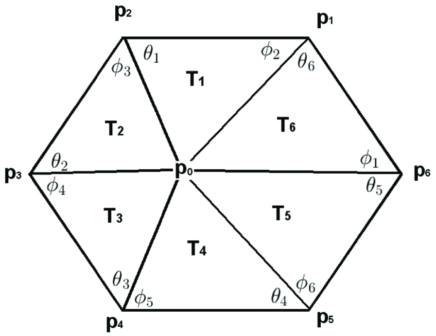
Let be neighboring vertices around the central vertex (Figure 3). Then the estimated Laplace-Beltrami operator is given by
| (18) |
with the weights
where and are the two angles opposite to the edge connecting and , and is the area of the -th triangle (Figure 3).
FEM estimation (18) is an improved formulation from the previous attempt in diffusion smoothing (Andrade et al., 2001), where the Laplacian is simply estimated as the planar Laplacian after locally flattening the triangular mesh consisting of nodes onto a flat plane. Afterwards, the finite difference (FD) scheme can be used to iteratively solve the diffusion equation at each vertex :
with the initial condition and fixed . After iterations, the FD gives the diffusion of the initial data after time . If the diffusion were applied to Euclidean space, it would be approximately equivalent to Gaussian kernel smoothing with
For large meshes, computing the linear weights for the Laplace-Beltrami operator takes a fair amount of time, but once the weights are computed, it is applied repeatedly throughout the iterations as a matrix multiplication. Unlike Gaussian kernel smoothing, diffusion smoothing is an iterative procedure.
5.2 Iterated Kernel Smoothing
Diffusion smoothing use FEM and FD, which are known to suffer numerical instability if sufficiently small step size is not chosen in the forward Euler scheme. To remedy the problem associated with diffusion smoothing, iterative kernel smoothing333MATLAB package: www.stat.wisc.edu/mchung/softwares/hk/hk.html. was introduced (Chung et al., 2005). The method has been used in smoothing various cortical surface data: cortical curvatures (Luders, Thompson, Narr, Toga, Jancke & Gaser, 2006; Gaser et al., 2006), cortical thickness (Luders, Narr, Thompson, Rex, Woods, DeLuca, Jancke & Toga, 2006; Bernal-Rusiel et al., 2008), hippocampus (Shen et al., 2006; Zhu et al., 2007), magnetoencephalography (MEG) (Han et al., 2007) and functional-MRI (Hagler Jr. et al., 2006; Jo et al., 2007). This and its variations are probably the most widely used method for smoothing brain surface data at this moment. In iterated kernel smoothing, kernel weights are spatially adapted to follow the shape of the heat kernel in a discrete fashion.
The -th iterated kernel smoothing of signal with kernel is defined as
where is the bandwidth of the kernel. If is a heat kernel, we have the following iterative relation (Chung et al., 2005):
| (19) |
The relation (19) shows that kernel smoothing with large bandwidth can be decomposed into repeated applications of kernel smoothing with smaller bandwidth . This idea can be used to approximate the heat kernel. When the bandwidth is small, the heat kernel behaves like the Dirac-delta function and, using the parametrix expansion (Rosenberg, 1997; Wang, 1997), we can approximate it locally using the Gaussian kernel.
Let be neighboring vertices of vertex in the mesh. The geodesic distance between and its adjacent vertex is the length of edge between these two vertices in the mesh. Then the discretized and normalized heat kernel is given by
Note . For small bandwidth, all the kernel weights are concentrated near the center, so we only need to worry about the first neighbors of a given vertex in a surface mesh. The discrete version of heat kernel smoothing on a triangle mesh is then given by
The discrete kernel smoothing should converge to heat kernel smoothing as the mesh resolution increases. This is the form of the Nadaraya-Watson estimator (Chaudhuri & Marron, 2000) in statistics. Instead of performing a single kernel smoothing with large bandwidth , we perform iterated kernel smoothing with small bandwidth as follows .
5.3 Heat Kernel Smoothing
The recently proposed heat kernel smoothing444MATLAB package: brainimaging.waisman.wisc.edu/chung/lb. framework constructs the heat kernel analytically using the eigenfunctions of the Laplace-Beltrami operator (Seo et al., 2010). This method avoids the need for the linear approximation used in iterative kernel smoothing that compounds the approximation error at each iteration. The method represents isotropic heat diffusion analytically as a series expansion so it avoids the numerical convergence issues associated with solving the diffusion equations numerically (Andrade et al., 2001; Chung, 2012; Joshi et al., 2009). This technique is different from other diffusion-based smoothing methods in that it bypasses the various numerical problems such as numerical instability, slow convergence, and accumulated linearization error.
Although recently there have been a few studies that introduce heat kernel in computer vision and machine learning (Belkin et al., 2006), they mainly use heat kernel to compute shape descriptors (Sun et al., 2009; Bronstein & Kokkinos, 2010) or to define a multi-scale metric (de Goes et al., 2008). These studies did not use heat kernel in smoothing functional data on manifolds. Further, most kernel methods in machine learning deal with the linear combination of kernels as a solution to penalized regressions, which significantly differs from the heat kernel smoothing framework, which does not have a penalized cost function. There are log-Euclidean and exponential map frameworks on manifolds, where the main interest is in computing the Fréchet mean along the tangent space (Davis et al., 2010; Fletcher et al., 2004). Such approaches or related methods in (Gerber et al., 2009), the Nadaya-Watson type of kernel regression is reformulated to learn the shape or image means in a population. In the heat kernel smoothing framework, we are not dealing with manifold data but scalar data defined on a manifold, so there is no need for exploiting the manifold structure of the data itself.
Let be the Laplace-Beltrami operator on . Solving the eigenvalue equation
| (20) |
we order eigenvalues
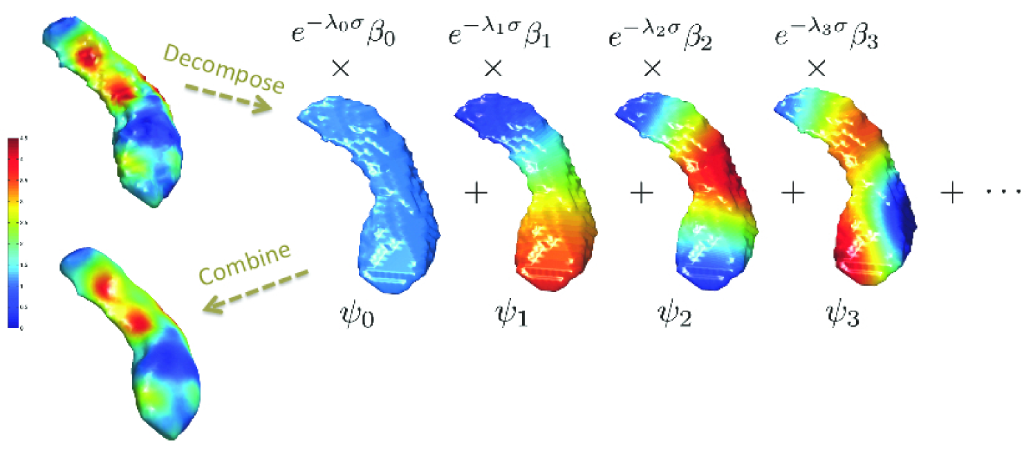
and corresponding eigenfunctions (Rosenberg, 1997; Chung et al., 2005; Lévy, 2006; Shi et al., 2009). The eigenfunctions form an orthonormal basis in , the space of square integrable functions in . Figure 4 shows the first four LB-eigenfunctions on a hippocampal surface.
There is extensive literature on the use of eigenvalues and eigenfunctions of the Laplace-Beltrami operator in medical imaging and computer vision (Lévy, 2006; Qiu et al., 2006; Reuter et al., 2009; Reuter, 2010; Zhang et al., 2007, 2010). The eigenvalues have been used in caudate shape discriminators (Niethammer et al., 2007). Qiu et al. used eigenfunctions in constructing splines on cortical surfaces (Qiu et al., 2006). Reuter used the topological features of eigenfunctions (Reuter, 2010). Shi et al. used the Reeb graph of the second eigenfunction in shape characterization and landmark detection in cortical and subcortical structures (Shi et al., 2008, 2009). Lai et al. used the critical points of the second eigenfunction as anatomical landmarks for colon surfaces (Lai et al., 2010).
Using the eigenfunctions, heat kernel is defined as
| (21) |
where is the bandwidth of the kernel. The heat kernel is the generalization of a Gaussian kernel. Then heat kernel smoothing of functional measurement is defined as
| (22) |
where are Fourier coefficients (Chung et al., 2005). Kernel smoothing is taken as the estimate for the unknown mean signal . The degree for truncating the series expansion can be automatically determined using the forward model selection procedure (Chung et al., 2008). Figure 4 shows the heat kernel smoothing results with the bandwidth and number of LB-eigenfunctions.
Unlike previous approaches to heat diffusion (Andrade et al., 2001; Chung, 2012; Joshi et al., 2009; Tasdizen et al., 2006), heat kernel smoothing avoids the direct numerical discretization of the diffusion equation. Instead, we discretize the basis functions of given manifold by solving for the eigensystem (20) and obtain and . This provides more robust stable smoothing results compared to diffusion smoothing or iterated kernel smoothing approaches.
6 Statistical Inference on Surfaces
Surface measurements such as cortical thickness, curvatures, or fMRI responses can be modeled as random fields on the cortical surface:
| (23) |
where the deterministic part is the unknown mean of the observed functional measurement and is a mean zero random field. The functional measurements on the brain surface is often modeled using the general linear models (GLMs) or its multivariate version. Various statistical models are proposed for estimating and modeling the signal component (Joshi et al., 1995; Chung, 2012; Chung et al., 2008) but the majority of the methods are all based on GLM. GLMs have been implemented in the brain image analysis packages such as SPM and fMRISTAT555The fMRISTAT package is available at www.math.mcgill.ca/keith/fmristat..
6.1 General Linear Models
We set up a GLM at each mesh vertex. Let be the response variable, which is mainly coming from images and to be the variables of interest and to be nuisance variables corresponding to the -th subject. Assume there are subjects, i.e., . We are interested in testing the significance of variables while accounting for nuisance covariates . Then we set up GLM
where and are unknown parameter vectors to be estimated. We assume to be the usual zero mean Gaussian noise, although the distributional assumption is not required for the least squares estimation. We test hypotheses
Subsequently the inference is done by constructing the -statistic with and degrees of freedom. GLMs have been used in quantifying cortical thickness, for instance, in child development (Chung, 2012; Chung et al., 2005) and amygdala shape differences in autism (Chung, 2012).
In the hippocampus case study, the first T1-weighted MRI scans are taken at years for children using a 3T GE SIGNA scanner. Variables age and gender are available. We also have variable income, which is a binary dummy variable indicating whether the subjects are from high- or low-income families. A total of 124 children and adolescents are from high- (; ) and low-income (, ) parents respectively. In addition to this cross-sectional data, longitudinal data was available for 82 of these subjects (, ; , ). The second MRI scan was acquired for these 82 subjects about 2 years later at years. For now, we will simply ignore the correlation between the scans within a subject and will treat them as independent.
On the template surface, we have the displacement vector fields of mapping from the template to individual subjects (Figure 2). We take the length of the surface displacement, denoted as deformation, with respect to the template as the response variable. The displacement measures the shape difference with respect to the template. However, since the length measurement is noisy, surface-based smoothing is necessary. We have used heat kernel smoothing to smooth out noise with the bandwidth 1 and 500 LB-eigenfunctions. Then we set up the GLM:
and test for the significance of at each mesh vertex. Figure 5-left shows the -statistic result on testing .
6.2 Multivariate General Linear Models
The multivariate general linear models (MGLMs) have been also used in modeling multivariate imaging features on brain surfaces. These models generalize a widely used univariate GLM by incorporating vector valued responses and explanatory variables (Anderson, 1984; Friston et al., 1995; Worsley et al., 1996, 2004; Taylor & Worsley, 2008; Chung, 2012). Hotelling’s statistic is a special case of MGLM that has been used primarily for inference on surface shapes, deformations and multi-scale features (Cao & Worsley, 1999; Chung, 2012; Gaser et al., 1999; Joshi, 1998; Kim et al., 2012; Thompson et al., 1997). An example of this approach is Hotelling’s -statistic applied in determining the 3D brain morphology of HIV/AIDS patients (Lepore et al., 2006). Hotelling’s -statistic is also applied to 2D deformation tensor at each mesh vertex on the hippocampal surface as a way to characterize AlzheimerÕs diseases (Wang et al., 2011).
Suppose there are a total of subjects and multivariate features of interest at each voxel. For MGLM to work, should be significantly larger than . Let be the measurement matrix, where is the measurement for subject and for the -th feature. The subscripts denote the dimension of the matrix. All the measurements over subjects for the -th feature are denoted as . The measurement vector for the -th subject is denoted as . is expected to be distributed identically and independently over subjects. Note that
We may assume the covariance matrix of to be
With these notations, we now set up the following MGLM at each mesh vertex:
| (24) |
is the matrix of contrasted explanatory variables while is the matrix of unknown coefficients. Nuisance covariates are in matrix and the corresponding coefficients are in matrix . The components of Gaussian random matrix are independently distributed with zero mean and unit variance. Symmetric matrix is the square root of the covariance matrix accounting for the spatial dependency across different voxels. In MGLM (24), we are usually interested in testing hypotheses
The parameter matrices in the model are estimated via the least squares method. The multivariate test statistics such as Lawley-Hotelling trace or Roy’s maximum root are used to test the significance of . When there is only one voxel, i.e. , these multivariate test statistics collapse to Hotelling’s statistic (Worsley et al., 2004; Chung, 2012).
6.3 Small- Large- Problems
GLM are usually fitted in each voxel separately. Instead of fitting GLM at each voxel, one may be tempted to fit the model in the whole brain surface. For FreeSurfer meshes, we need to fit GLM over 300000 vertices, which causes the small- large- problem (Friston et al., 1995; Schäfer & Strimmer, 2005; Chung, 2013).
Let be the measurement vector at the -th vertex. Assume there are subjects and total vertices in the surface. We have the same design matrix for all vertices. Then we need to estimate the parameter vector in
| (25) |
for each . Instead of solving (25) separately at each vertex, we combine all of them together so that we have matrix equation
| (26) |
The least squares estimation of the parameter matrix is given by
Note that is of size by and is only invertible when . The least squares estimation does not provide robust parameter estimates for , which is the usual case in surface modeling. For small- large- problem, GLM need to be regularized using the L1-norm penalty (Banerjee et al., 2006, 2008; Chung, 2013; Friedman et al., 2008; Huang et al., 2010; Mazumder & Hastie, 2012).
6.4 Longitudinal Models
So far we have only dealt with an imaging data set where the parameters of the model are fixed and do not vary across subjects and scans. Such fixed-effects models are inadequate in modeling the within-subject dependency in longitudinally collected imaging data. However, mixed-effects models can explicitly model such dependency (Fox, 2002; Milliken & Edland, 2000; Molenberghs & Verbeke, 2005; Pinehiro & Bates, 2002). There are three advantages of the mixed-effects model over the usual fixed-effects model. It explicitly models individual growth patterns and accommodates an unequal number of follow-up image scans per subject and unequal time intervals between scans.
The longitudinal outcome from the -th subject is modeled using the mixed-effects model (Milliken & Edland, 2000) as
| (27) |
where is the fixed-effects shared by all subjects. is the subject-specific random-effects and is independent and identically distributed noise. and are the design matrices corresponding to the fixed and random effects respectively for the -th subject. We assume and with some covariance matrices and . Hierarchically we are modeling (27) as
accounts for covariance among random effect terms. The within-subject variability between the scans is expected to be smaller than between-subject variability and explicitly modeled by . The covariance of and are expected to have block diagonal structure such that there is no correlation among the scans of different subjects while there is high correlation between the scans of the same subject:
Subsequently, the overall covariance of is given by
The random-effect contribution is while the within-subject contribution is .
The parameters and the covariance matrices can be estimated via the restricted maximum likelihood (REML) method (Fox, 2002; Pinehiro & Bates, 2002). The most widely used tools for fitting the mixed-effects model are the nlme library in the R statistical package (Pinehiro & Bates, 2002). However, there is no need to use R to fit the mixed-effects model. Keith Worsley has implemented the REML procedure in the SurfStat package666The MATLAB package is available at www.math.mcgill.ca/keith/surfstat. (Chung, 2012; Worsley et al., 2009).
Here we briefly explain how to set up a longitudinal mixed-effect model in practice. In the usual fixed-effect model, we have a linear model containing the fixed-effect term for the -th subject:
| (28) |
where is assumed to follow independent Gaussian. In (28), every subject has identical growth trajectory , which is unrealistic. Biologically, each subject is expected to have its own unique growth trajectory. So we assume each subject to have its own intercept and slope :
| (29) |
It is reasonable to assume the random vector to be multivariate normal. The model (29) can be decomposed into fixed- and random-effect terms:
| (30) |
The fixed-effect term models the linear growth of the population while the random-effect term models the subject specific growth variations. Incorporating additional factors and interaction terms are done similarly.
In the hippocampus case study, the first MRI scans are taken at years while the second scans are taken at years. We are interested in determining the effects of income level on the shape of the hippocampus. In Section 6.1, we treated the second scans as if they came from independent subjects and modeled them using the fixed-effects model. Now we explicitly incorporate the dependency of repeated scans of the same subject. It is necessary to explicitly model the within-subject variability that is expected to be smaller than between-subject variability. This can be done by introducing a random-effect term. The resulting F-statistic maps are given in Figure 5-right. However, we did not detect any region that is affected by income. Thus, we tested the age and income interaction and found the regions of strong interaction (Figure 6).
6.5 Random Field Theory
Since we need to set up a GLM on every mesh vertex, it becomes a multiple comparisons problem. Correcting for multiple comparisons is crucial in determining overall statistical significance in correlated test statistics over the whole surface. For surface data, various methods are proposed: Bonferroni correction, random field theory (Worsley, 1994; Worsley et al., 1996), false discovery rates (FDR) (Benjamini & Hochberg, 1995; Benjamini & Yekutieli, 2001; Genovese et al., 2002), and permutation tests (Nichols & Holmes, 2002). Among many techniques, the random field theory is probably the most natural in relation to surface data smoothing since it is able to explicitly control the amount of smoothing.
The generalization of a continuous stochastic process in to a higher dimensional abstract space is called a random field (Adler & Taylor, 2007; Chung, 2012; Dougherty, 1999; Joshi, 1998; Yaglom, 1987). In the random field theory (Worsley, 1994; Worsley et al., 1996), measurement at position is modeled as
where is the unknown signal to be estimated and is the measurement error. The measurement error at each fixed can be modeled as a random variable. Then the collection of random variables is called a random field or stochastic process. A measure-theoretic definition is given in (Adler & Taylor, 2007).
Detecting the regions of statistically significant for some can be done via thresholding the maximum of a random field defined on the cortical surface (Worsley et al., 1996, 1999). For instance, random field on the surface is defined as
where and are the sample mean and standard deviation over the subjects. Under the null hypothesis
is distributed as a student’s with degrees of freedom at each voxel . The pvalue of the local maxima of the field will give a conservative threshold compared to FDR (Worsley et al., 1996).
For sufficiently high threshold , we can show that
| (31) |
where is the -dimensional EC-density and the Minkowski functional are
and is the total surface area of (Worsley, 1996a). When diffusion or heat kernel smoothing with given FWHM is applied on surface , the 0-dimensional and 2-dimensional EC-density becomes
The excursion probability, which is the probability of obtaining false positives for the one-sided alternate hypothesis, is approximated by the following formula:
For smoothing cortical thickness (Chung, 2012; Chung et al., 2005), an FWHM of between 20 to 30 mm is recommended. This FWHM reflects the spatial frequency associated with the sulcal pattern. For measurements on smaller subcortical structures such as hippocampus and amygdala, significantly smaller FWHM is recommended. For amygdala and hippocampus, 0.5–1 mm would be sufficient.
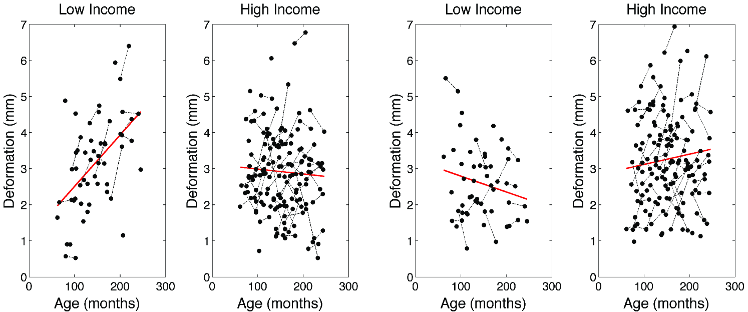
In the hippocampus case study, we did not detect any statistically significant group difference at 0.01 level after correcting for multiple comparisons in both the left and right hippocampi. However, we obtained highly focalized regions of group difference in the growth rate, the interaction between income level and age, in the right hippocampus (corrected pvalue = 0.03). The posterior region is enlarging while the midbody and the anterior parts are shrinking in children from low-income families (Figure 6 and 7). On the other hand, the pattern is opposite for children from high-income families. Note that the right hippocampus is involved in the active maintenance of associations with spatial information (Piekema et al., 2006). Future studies investigating the relationship between family socioeconomic status and spatial information processing measures are warranted.
Acknowledgements
This study was supported by NIH grants UL1TR000427, MH61285 and MH68858, EB022856 and EB028753, and NSF grant MDS-2010778.
References
- (1)
- Adler & Taylor (2007) Adler, R. & Taylor, J. (2007), Random Fields and Geometry, Springer Verlag.
- Anderson (1984) Anderson, T. (1984), An Introduction to Multivariate Statistical Analysis, 2nd edn, Wiley.
- Andrade et al. (2001) Andrade, A., Kherif, F., Mangin, J., Worsley, K., Paradis, A., Simon, O., Dehaene, S., Le Bihan, D. & Poline, J.-B. (2001), ‘Detection of fMRI activation using cortical surface mapping’, Human Brain Mapping 12, 79–93.
- Angenent et al. (1999) Angenent, S., Hacker, S., Tannenbaum, A. & Kikinis, R. (1999), ‘On the Laplace-Beltrami operator and brain surface flattening’, IEEE Transactions on Medical Imaging 18, 700–711.
- Arfken (2000) Arfken, G. (2000), Mathematical Methods for Physicists, 5th edn, Academic Press.
- Avants et al. (2008) Avants, B., Epstein, C., Grossman, M. & Gee, J. (2008), ‘Symmetric diffeomorphic image registration with cross-correlation: Evaluating automated labeling of elderly and neurodegenerative brain’, Medical Image Analysis 12, 26–41.
- Banerjee et al. (2008) Banerjee, O., El Ghaoui, L. & d’Aspremont, A. (2008), ‘Model selection through sparse maximum likelihood estimation for multivariate Gaussian or binary data’, The Journal of Machine Learning Research 9, 485–516.
- Banerjee et al. (2006) Banerjee, O., Ghaoui, L., d’Aspremont, A. & Natsoulis, G. (2006), Convex optimization techniques for fitting sparse Gaussian graphical models, in ‘Proceedings of the 23rd International Conference on Machine Learning’, p. 96.
- Barta et al. (2005) Barta, P., Miller, M. & Qiu, A. (2005), ‘A stochastic model for studying the laminar structure of cortex from mri’, IEEE Transactions on Medical Imaging 24, 728–742.
- Bartesaghi & Sapiro (2001) Bartesaghi, A. & Sapiro, G. (2001), ‘A system for the generation of curves on 3d brain images’, Human Brain Mapping 14(1), 1–15.
- Belkin et al. (2006) Belkin, M., Niyogi, P. & Sindhwani, V. (2006), ‘Manifold regularization: A geometric framework for learning from labeled and unlabeled examples’, The Journal of Machine Learning Research 7, 2399–2434.
- Benjamini & Hochberg (1995) Benjamini, Y. & Hochberg, Y. (1995), ‘Controlling the false discovery rate: A practical and powerful approach to multiple testing’, Journal of Royal Statistical Society, Series. B 57, 289–300.
- Benjamini & Yekutieli (2001) Benjamini, Y. & Yekutieli, D. (2001), ‘The control of the false discovery rate in multiple testing under dependency’, Annals of Statistics 29, 1165–1188.
- Bernal-Rusiel et al. (2008) Bernal-Rusiel, J., Atienza, M. & Cantero, J. (2008), ‘Detection of focal changes in human cortical thickness: Spherical wavelets versus gaussian smoothing’, NeuroImage 41, 1278–1292.
- Blanco et al. (1997) Blanco, M., Florez, M. & Bermejo, M. (1997), ‘Evaluation of the rotation matrices in the basis of real spherical harmonics’, Journal of Molecular Structure: THEOCHEM 419, 19–27.
- Boothby (1986) Boothby, W. (1986), An Introduction to Differential Manifolds and Riemannian Geometry, 2nd edn, Academic Press, London.
- Brechbuhler et al. (1995) Brechbuhler, C., Gerig, G. & Kubler, O. (1995), ‘Parametrization of closed surfaces for 3d shape description’, Computer Vision and Image Understanding 61, 154–170.
- Bronstein & Kokkinos (2010) Bronstein, M. M. & Kokkinos, I. (2010), Scale-invariant heat kernel signatures for non-rigid shape recognition, in ‘IEEE Conference on Computer Vision and Pattern Recognition (CVPR)’, pp. 1704–1711.
- Bulow (2004) Bulow, T. (2004), ‘Spherical diffusion for 3D surface smoothing’, IEEE Transactions on Pattern Analysis and Machine Intelligence 26, 1650–1654.
- Cachia, Mangin, Riviére, Kherif, Boddaert, Andrade, Papadopoulos-Orfanos, Poline, Bloch, Zilbovicius, Sonigo, Brunelle & Régis (2003) Cachia, A., Mangin, J.-F., Riviére, D., Kherif, F., Boddaert, N., Andrade, A., Papadopoulos-Orfanos, D., Poline, J.-B., Bloch, I., Zilbovicius, M., Sonigo, P., Brunelle, F. & Régis, J. (2003), ‘A primal sketch of the cortex mean curvature: A morphogenesis based approach to study the variability of the folding patterns’, IEEE Transactions on Medical Imaging 22, 754–765.
- Cachia, Mangin, Riviére, Papadopoulos-Orfanos, Kherif, Bloch & Régis (2003) Cachia, A., Mangin, J.-F., Riviére, D., Papadopoulos-Orfanos, D., Kherif, F., Bloch, I. & Régis, J. (2003), ‘A generic framework for parcellation of the cortical surface into gyri using geodesic Voronoï diagrams’, Image Analysis 7, 403–416.
- Cao & Worsley (1999) Cao, J. & Worsley, K. (1999), ‘The detection of local shape changes via the geometry of Hotelling’s T2 fields’, Annals of Statistics 27, 925–942.
- Chaudhuri & Marron (2000) Chaudhuri, P. & Marron, J. (2000), ‘Scale space view of curve estimation’, The Annals of Statistics 28, 408–428.
- Chung (2012) Chung, M. (2012), Computational Neuroanatomy: The Methods, World Scientific, Singapore.
- Chung (2013) Chung, M. (2013), Statistical and Computational Methods in Brain Image Analysis, CRC Press.
- Chung et al. (2011) Chung, M., Hanson, J., Davidson, R. & Pollak, S. (2011), ‘Effect of family income on hippocampus growth: Longitudinal study’, 17th Annual Meeting of the Organization for Human Brain Mapping (2697).
- Chung et al. (2008) Chung, M., Hartley, R., Dalton, K. & Davidson, R. (2008), ‘Encoding cortical surface by spherical harmonics’, Statistica Sinica 18, 1269–1291.
- Chung et al. (2005) Chung, M., Robbins, S. & Evans, A. (2005), ‘Unified statistical approach to cortical thickness analysis’, Information Processing in Medical Imaging (IPMI), Lecture Notes in Computer Science 3565, 627–638.
- Chung et al. (n.d.) Chung, M., Schaefer, S., van Reekum, C. M., Schmitz, L., Sutterer, M. & Davidson, R. (n.d.), ‘A unified kernel regression on manifolds detects aging-related changes in the amygdala and hippocampus’, MICCAI, Lecture Notes in Computer Science (LNCS) 8674, 789–796.
- Chung et al. (2003) Chung, M., Worsley, K., Robbins, S., Paus, T., Taylor, J., Giedd, J., Rapoport, J. & Evans, A. (2003), ‘Deformation-based surface morphometry applied to gray matter deformation’, NeuroImage 18, 198–213.
- Chung et al. (2001) Chung, M., Worsley, K., Taylor, J., Ramsay, J., Robbins, S. & Evans, A. (2001), ‘Diffusion smoothing on the cortical surface’, NeuroImage 13, S95.
- Courant & Hilbert (1953) Courant, R. & Hilbert, D. (1953), Methods of Mathematical Physics, English edn, Interscience, New York.
- Dale & Fischl (1999) Dale, A. & Fischl, B. (1999), ‘Cortical surface-based analysis I. Segmentation and surface reconstruction’, NeuroImage 9, 179–194.
- Davatzikos (1997) Davatzikos, C. (1997), ‘Spatial transformation and registration of brain images using elastically deformable models’, Comput. Vis. Image Understanding 66, 207–222.
- Davatzikos & Bryan (1995) Davatzikos, C. & Bryan, R. (1995), ‘Using a deformable surface model to obtain a shape representation of the cortex’, Proceedings of the IEEE International Conference on Computer Vision 9, 2122–2127.
- Davis et al. (2010) Davis, B., Fletcher, P., Bullitt, E. & Joshi, S. (2010), ‘Population shape regression from random design data’, International Journal of Computer Vision 90, 255–266.
- de Goes et al. (2008) de Goes, F., Goldenstein, S. & Velho, L. (2008), ‘A hierarchical segmentation of articulated bodies’, Computer Graphics Forum 27, 1349–1356.
- do Carmo (1992) do Carmo, M. (1992), Riemannian Geometry, Prentice-Hall, Inc.
- Dougherty (1999) Dougherty, E. (1999), Random Processes for Image and Signal Processing, IEEE Press.
- Dupuis et al. (1998) Dupuis, P., Grenander, U. & Miller, M. I. (1998), ‘Variational problems on flows of diffeomorphisms for image matching’, Quarterly of Applied Math. 56, 587–600.
- Fischl & Dale (2000) Fischl, B. & Dale, A. (2000), ‘Measuring the thickness of the human cerebral cortex from magnetic resonance images’, Proceedings of the National Academy of Sciences (PNAS) 97, 11050–11055.
- Fischl et al. (1999) Fischl, B., Sereno, M., Tootell, R. & Dale, A. (1999), ‘High-resolution intersubject averaging and a coordinate system for the cortical surface’, Hum. Brain Mapping 8, 272–284.
- Fletcher et al. (2004) Fletcher, P., Lu, C., Pizer, S. & Joshi, S. (2004), ‘Principal geodesic analysis for the study of nonlinear statistics of shape’, IEEE Transactions on Medical Imaging 23, 995–1005.
- Fox (2002) Fox, J. (2002), An R and S-Plus Companion to Applied Regression, Sage Publications, Inc.
- Friedman et al. (2008) Friedman, J., Hastie, T. & Tibshirani, R. (2008), ‘Sparse inverse covariance estimation with the graphical lasso.’, Biostatistics 9, 432.
- Friston et al. (1995) Friston, K., Holmes, A., Worsley, K., Poline, J.-P., Frith, C. & Frackowiak, R. (1995), ‘Statistical parametric maps in functional imaging: A general linear approach’, Human Brain Mapping 2, 189–210.
- Gaser et al. (2006) Gaser, C., Luders, E., Thompson, P., Lee, A., Dutton, R., Geaga, J., Hayashi, K., Bellugi, U., Galaburda, A., Korenberg, J., Mills, D., Toga, A. & Reiss, A. (2006), ‘Increased local gyrification mapped in Williams syndrome’, NeuroImage 33, 46–54.
- Gaser et al. (1999) Gaser, C., Volz, H.-P., Kiebel, S., Riehemann, S. & Sauer, H. (1999), ‘Detecting structural changes in whole brain based on nonlinear deformations - Application to schizophrenia research’, NeuroImage 10, 107–113.
- Gelb (1997) Gelb, A. (1997), ‘The resolution of the Gibbs phenomenon for spherical harmonics’, Mathematics of Computation 66, 699–717.
- Genovese et al. (2002) Genovese, C., Lazar, N. & Nichols, T. (2002), ‘Thresholding of statistical maps in functional neuroimaging using the false discovery rate’, NeuroImage 15, 870–878.
- Gerber et al. (2009) Gerber, S., Tasdizen, T. & Whitaker, R. (2009), Dimensionality reduction and principal surfaces via kernel map manifolds, in ‘IEEE 12th International Conference on Computer Vision (ICCV)’, pp. 529–536.
- Gerig et al. (2001) Gerig, G., Styner, M., Jones, D., Weinberger, D. & Lieberman, J. (2001), Shape analysis of brain ventricles using SPHARM, in ‘MMBIA’, pp. 171–178.
- Good et al. (2001) Good, C., Johnsrude, I., Ashburner, J., Henson, R., Friston, K. & Frackowiak, R. (2001), ‘A voxel-based morphometric study of ageing in 465 normal adult human brains’, NeuroImage 14, 21–36.
- Griffin (1994) Griffin, L. (1994), ‘The intrinsic geometry of the cerebral cortex’, Journal of Theoretical Biology 166, 261–273.
- Gu et al. (2004) Gu, X., Wang, Y., Chan, T., Thompson, T. & Yau, S. (2004), ‘Genus zero surface conformal mapping and its application to brain surface mapping’, IEEE Transactions on Medical Imaging 23, 1–10.
- Hagler Jr. et al. (2006) Hagler Jr., D., Saygin, A. & Sereno, M. (2006), ‘Smoothing and cluster thresholding for cortical surface-based group analysis of fMRI data’, NeuroImage 33, 1093–1103.
- Han et al. (2007) Han, J., Kim, J., Chung, C. & Park, K. (2007), ‘Evaluation of smoothing in an iterative lp-norm minimization algorithm for surface-based source localization of meg’, Physics in Medicine and Biology 52, 4791–4803.
- Henery & Mayhew (1989) Henery, C. & Mayhew, T. (1989), ‘The cerebrum and cerebellum of the fixed human brain: Efficient and unbiased estimates of volumes and cortical surface areas.’, Journal of Anatomy 167, 167–180.
- Homeier & Steinborn (1996) Homeier, H. & Steinborn, E. (1996), ‘Some properties of the coupling coefficients of real spherical harmonics and their relation to gaunt coefficients’, Journal of Molecular Structure: THEOCHEM 368, 31–37.
- Hosseinbor et al. (2014) Hosseinbor, A., Kim, W., Adluru, N., Acharya, A., Vorperian, H. & Chung, M. (2014), The 4D hyperspherical diffusion wavelet: A new method for the detection of localized anatomical variation, in ‘International Conference on Medical Image Computing and Computer-Assisted Intervention’, Vol. 8675, pp. 65–72.
- Huang et al. (2010) Huang, S., Li, J., Sun, L., Ye, J., Fleisher, A., Wu, T., Chen, K. & Reiman, E. (2010), ‘Learning brain connectivity of Alzheimer’s disease by sparse inverse covariance estimation’, NeuroImage 50, 935–949.
- Hurdal & Stephenson (2004) Hurdal, M. K. & Stephenson, K. (2004), ‘Cortical cartography using the discrete conformal approach of circle packings’, NeuroImage 23, S119–S128.
- Jo et al. (2007) Jo, H., Lee, J.-M., Kim, J.-H., Shin, Y.-W., Kim, I.-Y., Kwon, J. & Kim, S. (2007), ‘Spatial accuracy of fmri activation influenced by volume- and surface-based spatial smoothing techniques’, NeuroImage 34, 550–564.
- Jones et al. (2000) Jones, S., Buchbinder, B. & Aharon, I. (2000), ‘Three-dimensional mapping of cortical thickness using Laplace’s equation’, Human Brain Mapping 11, 12–32.
- Joshi et al. (2009) Joshi, A., Shattuck, D. W., Thompson, P. M. & Leahy, R. M. (2009), ‘A parameterization-based numerical method for isotropic and anisotropic diffusion smoothing on non-flat surfaces’, IEEE Transactions on Image Processing 18, 1358–1365.
- Joshi (1998) Joshi, S. (1998), Large Deformation Diffeomorphisms and Gaussian Random Fields for Statistical Characterization of Brain Sub-Manifolds, PhD thesis, Washington University, St. Louis.
- Joshi et al. (1995) Joshi, S., Wang, J., Miller, M., Van Essen, D. & Grenander, U. (1995), Differential geometry of the cortical surface, in ‘Vision Geometry IV, Vol. 2573, Proceedings of the SPIE 1995 International Symposium on Optical Science, Engineering and Instrumentation’, pp. 304–311.
- Kelemen et al. (1999) Kelemen, A., Szekely, G. & Gerig, G. (1999), ‘Elastic model-based segmentation of 3-d neuroradiological data sets’, IEEE Transactions on Medical Imaging 18, 828–839.
- Khaneja et al. (1998) Khaneja, N., Miller, M. & Grenander, U. (1998), ‘Dynamic programming generation of curves on brain surfaces’, IEEE Transactions on Pattern Analysis and Machine Intelligence 20, 1260–1265.
- Kim et al. (2012) Kim, W., Pachauri, D., Hatt, C., Chung, M., Johnson, S. & Singh, V. (2012), Wavelet based multi-scale shape features on arbitrary surfaces for cortical thickness discrimination, in ‘Advances in Neural Information Processing Systems’, pp. 1250–1258.
- Kollakian (1996) Kollakian, K. (1996), Performance analysis of automatic techniques for tissue classification in magnetic resonance images of the human brain, Technical Report Master’s thesis, Concordia University, Montreal, Quebec, Canada.
- Kreyszig (1959) Kreyszig, E. (1959), Differential Geometry, University of Toronto Press.
- Lai et al. (2010) Lai, Z., Hu, J., Liu, C., Taimouri, V., Pai, D., Zhu, J., Xu, J. & Hua, J. (2010), Intra-patient supine-prone colon registration in CT colonography using shape spectrum, in ‘Medical Image Computing and Computer-Assisted Intervention — MICCAI 2010’, Vol. 6361 of Lecture Notes in Computer Science, pp. 332–339.
- Lepore et al. (2006) Lepore, N., Brun, C., Chiang, M., Chou, Y., Dutton, R., Hayashi, K., Lopez, O., Aizenstein, H., Toga, A., Becker, J. & Thompson, P. (2006), ‘Multivariate statistics of the Jacobian matrices in tensor based morphometry and their application to HIV/AIDS’, Lecture Notes in Computer Science 4190, 191–198.
- Lévy (2006) Lévy, B. (2006), Laplace-Beltrami eigenfunctions towards an algorithm that “understands” geometry, in ‘IEEE International Conference on Shape Modeling and Applications’, p. 13.
- Lorensen & Cline (1987) Lorensen, W. & Cline, H. (1987), Marching cubes: A high resolution 3D surface construction algorithm, in ‘Proceedings of the 14th Annual Conference on Computer Graphics and Interactive Techniques’, pp. 163–169.
- Luders, Narr, Thompson, Rex, Woods, DeLuca, Jancke & Toga (2006) Luders, E., Narr, K., Thompson, P., Rex, D., Woods, R., DeLuca, H., Jancke, L. & Toga, A. (2006), ‘Gender effects on cortical thickness and the influence of scaling’, Human Brain Mapping 27, 314–324.
- Luders, Thompson, Narr, Toga, Jancke & Gaser (2006) Luders, E., Thompson, P., Narr, K., Toga, A., Jancke, L. & Gaser, C. (2006), ‘A curvature-based approach to estimate local gyrification on the cortical surface’, NeuroImage 29, 1224–1230.
- MacDonald et al. (2000) MacDonald, J., Kabani, N., Avis, D. & Evans, A. (2000), ‘Automated 3-D extraction of inner and outer surfaces of cerebral cortex from MRI’, NeuroImage 12, 340–356.
- Mallat & Zhang (1993) Mallat, S. & Zhang, Z. (1993), ‘Matching pursuits with time-frequency dictionaries’, IEEE Transactions on Signal Processing 41, 3397–3415.
- Mazumder & Hastie (2012) Mazumder, R. & Hastie, T. (2012), ‘Exact covariance thresholding into connected components for large-scale graphical LASSO’, The Journal of Machine Learning Research 13, 781–794.
- Miller et al. (1997) Miller, M., Banerjee, A., Christensen, G., Joshi, S., Khaneja, N., Grenander, U. & Matejic, L. (1997), ‘Statistical methods in computational anatomy’, Statistical Methods in Medical Research 6, 267–299.
- Miller & Qiu (2009) Miller, M. & Qiu, A. (2009), ‘The emerging discipline of computational functional anatomy’, NeuroImage 45(1S), S16–S39.
- Milliken & Edland (2000) Milliken, J. & Edland, S. (2000), ‘Mixed effect models of longitudinal Alzheimer’s disease data: A cautionary note’, Statist. Med. 19, 1617–1629.
- Molenberghs & Verbeke (2005) Molenberghs, G. & Verbeke, G. (2005), Models for Discrete Longitudinal Data, Springer.
- Nichols & Holmes (2002) Nichols, T. & Holmes, A. (2002), ‘Nonparametric permutation tests for functional neuroimaging: A primer with examples’, Human Brain Mapping 15, 1–25.
- Niethammer et al. (2007) Niethammer, M., Reuter, M., Wolter, F., Bouix, S., Peinecke, N., Koo, M. & Shenton, M. (2007), ‘Global medical shape analysis using the Laplace-Beltrami spectrum’, Lecture Notes in Computer Science 4791, 850.
- Ozkan et al. (1993) Ozkan, M., Dawant, B. & Maciunas, R. (1993), ‘Neural-network-based segmentation of multi-modal medical images: a comparative and prospective study’, IEEE Transactions on Medical Imaging 12, 534–544.
- Perona & Malik (1990) Perona, P. & Malik, J. (1990), ‘Scale-space and edge detection using anisotropic diffusion’, IEEE Trans. Pattern Analysis and Machine Intelligence 12, 629–639.
- Piekema et al. (2006) Piekema, C., Kessels, R., Mars, R., Petersson, K. & Fernández, G. (2006), ‘The right hippocampus participates in short-term memory maintenance of object-location associations’, NeuroImage 33, 374–382.
- Pinehiro & Bates (2002) Pinehiro, J. & Bates, D. (2002), Mixed Effects Models in S and S-Plus, 3rd edn, Springer.
- Qiu et al. (2006) Qiu, A., Bitouk, D. & Miller, M. (2006), ‘Smooth functional and structural maps on the neocortex via orthonormal bases of the Laplace-Beltrami operator’, IEEE Transactions on Medical Imaging 25, 1296–1396.
- Qiu & Miller (2008) Qiu, A. & Miller, M. (2008), ‘Multi-structure network shape analysis via normal surface momentum maps’, NeuroImage 42, 1430–1438.
- Reuter (2010) Reuter, M. (2010), ‘Hierarchical shape segmentation and registration via topological features of Laplace-Beltrami eigenfunctions’, International Journal of Computer Vision 89, 287–308.
- Reuter et al. (2009) Reuter, M., Wolter, F.-E., Shenton, M. & Niethammer, M. (2009), ‘Laplace-Beltrami eigenvalues and topological features of eigenfunctions for statistical shape analysis’, Computer-Aided Design 41, 739–755.
- Robbins (2003) Robbins, S. (2003), Anatomical standardization of the human brain in Euclidean 3-Space and on the cortical 2-manifold., PhD thesis, School of Computer Science, McGill University, Montreal, Quebec, Canada.
- Rosenberg (1997) Rosenberg, S. (1997), The Laplacian on a Riemannian Manifold, Cambridge University Press.
- Rosenfeld & Kak (1982) Rosenfeld, A. & Kak, A. (1982), Digital Picture Processing, Academic Press, New York.
- Rusch et al. (2001) Rusch, B., Abercrombie, H., Oakes, T., Schaefer, S. & Davidson, R. (2001), ‘Hippocampal morphometry in depressed patients and control subjects: Relations to anxiety symptoms’, Biological Psychiatry 50, 960–964.
- Schäfer & Strimmer (2005) Schäfer, J. & Strimmer, K. (2005), ‘A shrinkage approach to large-scale covariance matrix estimation and implications for functional genomics’, Statistical Applications in Genetics and Molecular Biology 4, 32.
- Seo et al. (2010) Seo, S., Chung, M. & Vorperian, H. (2010), Heat kernel smoothing using Laplace-Beltrami eigenfunctions, in ‘Medical Image Computing and Computer-Assisted Intervention — MICCAI 2010’, Vol. 6363 of Lecture Notes in Computer Science, pp. 505–512.
- Sethian (2002) Sethian, J. (2002), Level Set Methods and Fast Marching Methods: Evolving Interfaces in Computational Geometry, Fluid Mechanics, Computer Vision and Material Science, Cambridge University Press.
- Shen & Chung (2006) Shen, L. & Chung, M. (2006), Large-scale modeling of parametric surfaces using spherical harmonics, in ‘Third International Symposium on 3D Data Processing, Visualization and Transmission (3DPVT)’, pp. 294–301.
- Shen et al. (2004) Shen, L., Ford, J., Makedon, F. & Saykin, A. (2004), ‘Surface-based approach for classification of 3d neuroanatomical structures’, Intelligent Data Analysis 8, 519–542.
- Shen et al. (2006) Shen, L., Saykin, A., Chung, M., Huang, H., Ford, J., Makedon, F., McHugh, T. & Rhodes, C. (2006), Morphometric analysis of genetic variation in hippocampal shape in mild cognitive impairment: Role of an il-6 promoter polymorphism, in ‘Life Science Society Computational Systems Bioinformatics Conference’.
- Shi et al. (2009) Shi, Y., Dinov, I. & Toga, A. W. (2009), Cortical shape analysis in the Laplace-Beltrami feature space, in ‘12th International Conference on Medical Image Computing and Computer Assisted Intervention (MICCAI 2009)’, Vol. 5762 of Lecture Notes in Computer Science (LNCS), pp. 208–215.
- Shi et al. (2008) Shi, Y., Lai, R., Kern, K., Sicotte, N., Dinov, I. & Toga, A. W. (2008), Harmonic surface mapping with Laplace-Beltrami eigenmaps, in ‘11th International Conference on Medical Image Computing and Computer Assisted Intervention (MICCAI 2008)’, Vol. 5242 of Lecture Notes in Computer Science (LNCS), pp. 147–154.
- Sled et al. (1988) Sled, J., Zijdenbos, A. & Evans, A. (1988), ‘A nonparametric method for automatic correction of intensity nonuniformity in mri data’, IEEE Transactions on Medical Imaging 17, 87–97.
- Styner et al. (2006) Styner, M., Oguz, I., Xu, S., Brechbuhler, C., Pantazis, D., Levitt, J., Shenton, M. & Gerig, G. (2006), Framework for the statistical shape analysis of brain structures using SPHARM-PDM, in ‘Insight Journal, Special Edition on the Open Science Workshop at MICCAI’.
- Sun et al. (2009) Sun, J., Ovsjanikov, M. & Guibas, L. J. (2009), ‘A concise and provably informative multi-scale signature based on heat diffusion.’, Comput. Graph. Forum 28, 1383–1392.
- Tasdizen et al. (2006) Tasdizen, T., Whitaker, R., Burchard, P. & Osher, S. (2006), Geometric surface smoothing via anisotropic diffusion of normals, in ‘Geometric Modeling and Processing’, pp. 687–693.
- Taylor & Worsley (2008) Taylor, J. & Worsley, K. (2008), ‘Random fields of multivariate test statistics, with applications to shape analysis’, Annals of Statistics 36, 1–27.
- Thompson et al. (2000) Thompson, P., Giedd, J., Woods, R., MacDonald, D., Evans, A. & Toga, A. (2000), ‘Growth patterns in the developing human brain detected using continuum-mechanical tensor mapping’, Nature 404, 190–193.
- Thompson et al. (1997) Thompson, P., MacDonald, D., Mega, M., Holmes, C., Evans, A. & Toga, A. (1997), ‘Detection and mapping of abnormal brain structure with a probabilistic atlas of cortical surfaces’, Journal of Computer Assisted Tomography 21, 567–581.
- Thompson & Toga (1996) Thompson, P. & Toga, A. (1996), ‘A surface-based technique for warping 3-dimensional images of the brain’, IEEE Transactions on Medical Imaging 15, 1–16.
- Timsari & Leahy (2000) Timsari, B. & Leahy, R. (2000), An optimization method for creating semi-isometric flat maps of the cerebral cortex, in ‘The Proceedings of SPIE, Medical Imaging’.
- Vaillant et al. (2007) Vaillant, M., Qiu, A., Glaunès, J. & Miller, M. (2007), ‘Diffeomorphic metric surface mapping in subregion of the superior temporal gyrus’, NeuroImage 34, 1149–1159.
- Wahba (1990) Wahba, G. (1990), Spline Models for Observational Data, SIAM, New York.
- Wang (1997) Wang, F.-Y. (1997), ‘Sharp explicit lower bounds of heat kernels’, Annals of Probability 24, 1995–2006.
- Wang et al. (2011) Wang, Y., Song, Y., Rajagopalan, P., An, T., Liu, K., Chou, Y., Gutman, B., Toga, A., Thompson, P. & the Alzheimer’s Disease Neuroimaging Initiative (2011), ‘Surface-based TBM boosts power to detect disease effects on the brain: An N= 804 ADNI study’, NeuroImage 56, 1993–2010.
- Worsley (1994) Worsley, K. (1994), ‘Local maxima and the expected Euler characteristic of excursion sets of , and fields.’, Advances in Applied Probability 26, 13–42.
- Worsley et al. (1999) Worsley, K., Andermann, M., Koulis, T., MacDonald, D. & Evans, A. (1999), ‘Detecting changes in nonisotropic images’, Human Brain Mapping 8, 98–101.
- Worsley et al. (1996) Worsley, K., Marrett, S., Neelin, P., Vandal, A., Friston, K. & Evans, A. (1996), ‘A unified statistical approach for determining significant signals in images of cerebral activation’, Human Brain Mapping 4, 58–73.
- Worsley et al. (2009) Worsley, K., Taylor, J., Carbonell, F., Chung, M., Duerden, E., Bernhardt, B., Lyttelton, O., Boucher, M. & Evans, A. (2009), ‘SurfStat: A MATLAB toolbox for the statistical analysis of univariate and multivariate surface and volumetric data using linear mixed effects models and random field theory’, NeuroImage 47, S102.
- Worsley et al. (2004) Worsley, K., Taylor, J., Tomaiuolo, F. & Lerch, J. (2004), ‘Unified univariate and multivariate random field theory’, NeuroImage 23, S189–195.
- Yaglom (1987) Yaglom, A. (1987), Correlation Theory of Stationary and Related Random Functions Vol. I: Basic Results, Springer-Verlag.
- Yang et al. (2011) Yang, X., Goh, A. & Qiu, A. (2011), ‘Locally linear diffeomorphic metric embedding (LLDME) for surface-based anatomical shape modeling.’, NeuroImage 56, 149–161.
- Zhang et al. (2007) Zhang, H., Avants, B., Yushkevich, P., Woo, J., Wang, S., McCluskey, L., Elman, L., Melhem, E. & Gee, J. (2007), ‘High-dimensional spatial normalization of diffusion tensor images improves the detection of white matter differences: an example study using amyotrophic lateral sclerosis’, IEEE Transactions on Medical Imaging 26(11), 1585–1597.
- Zhang et al. (2010) Zhang, H., van Kaick, O. & Dyer, R. (2010), ‘Spectral mesh processing’, Computer Graphics Forum 29, 1865–1894.
- Zhu et al. (2007) Zhu, H., Ibrahim, J., Tang, N., Rowe, D., Hao, X., Bansal, R. & Peterson, B. (2007), ‘A statistical analysis of brain morphology using wild bootstrapping’, IEEE Transactions on Medical Imaging 26, 954–966.