[1]\fnmFei \surSha [1]\fnmLeonardo\surZepeda-Núñez
1]\orgdivGoogle Research, \orgaddress\cityMountain View, \stateCA, \countryUSA 2]\orgdivCalifornia Institute of Technology, \orgaddress\cityPasadena, \stateCA, \countryUSA
Statistical Downscaling via High-Dimensional Distribution Matching with Generative Models
Abstract
Statistical downscaling is a technique used in climate modeling to increase the resolution of climate simulations. High-resolution climate information is essential for various high-impact applications, including natural hazard risk assessment. However, simulating climate at high resolution is intractable. Thus, climate simulations are often conducted at a coarse scale and then downscaled to the desired resolution. Existing downscaling techniques are either simulation-based methods with high computational costs, or statistical approaches with limitations in accuracy or application specificity. We introduce Generative Bias Correction and Super-Resolution (GenBCSR), a two-stage probabilistic framework for statistical downscaling that overcomes the limitations of previous methods. GenBCSR employs two transformations to match high-dimensional distributions at different resolutions: (i) the first stage, bias correction, aligns the distributions at coarse scale, (ii) the second stage, statistical super-resolution, lifts the corrected coarse distribution by introducing fine-grained details. Each stage is instantiated by a state-of-the-art generative model, resulting in an efficient and effective computational pipeline for the well-studied distribution matching problem. By framing the downscaling problem as distribution matching, GenBCSR relaxes the constraints of supervised learning, which requires samples to be aligned. Despite not requiring such correspondence, we show that GenBCSR surpasses standard approaches in predictive accuracy of critical impact variables, particularly in predicting the tails (99% percentile) of composite indexes composed of interacting variables, achieving up to 4-5 folds of error reduction.
Significance statement
Methods for downscaling coarse global climate projections to regional high resolution information fall into two categories: physics-based simulations that are computationally demanding and statistical approaches that doe not model high-dimensional distributions thus incapable of capturing important inter-variable spatio-temporal correlations. The proposed paradigm is powered by state-of-the-art generative models. It avoids the high computational cost of physical simulations, and is able to capture extreme events at the tails of the distributions more accurately than competing methods. Thus, our approach opens the door to downscaling large climate ensembles, enabling impact-relevant local climate risk assessments.
1 Introduction
Statistical downscaling is a crucial tool for studying and correlating simulations of complex dynamical systems at multiple spatio-temporal scales. For example, in climate simulations, the computational complexity of general circulation models (GCMs) [1] grows at least cubically111The number of horizontal degrees of freedom grows quadratically with resolution, while the number of time-steps increases linearly in order to satisfy the CFL condition [2]. with respect to the horizontal resolution, quickly becoming prohibitive [3]. This severely limits the resolution of long-running climate projections, the cornerstone of climate modeling, particularly as large ensembles are routinely required to assess the risk induced by climate change [4, 5], which are necessary to inform climate adaptation policies.
Consequently, climate data at impact-relevant scales needs to be downscaled from coarser lower-resolution models’ outputs. This is a challenging task: coarser models do not resolve small-scale dynamics, thus creating bias [6, 3, 7], and they lack the necessary physical details (for instance, orographic weather effects [8]) to be of practical use for regional or local climate impact studies [9, 10], including risk assessment of extreme weather events [11, 12] such as extreme flooding [13, 14], heat waves [15], or wildfires [16]. This has resulted in an acute need for high-resolution, fine-grained data for economic sectors likely to be impacted by such phenomena [17, 18, 19, 20]. In return, this need has spurred the development of downscaling techniques and frameworks [21, 22], including recent machine-learning based ones [23, 24, 25, 26, 27, 28, 29].
At the most abstract level, statistical downscaling [21, 22] learns a statistical map (e.g., quantile mapping or generalized linear regression) from low- to high-resolution data. However, it poses several unique challenges. First, unlike supervised machine learning (ML), there is typically no natural pairing of samples from the low-resolution model (such as climate models [30]) with samples from higher-resolution ones (such as weather models that assimilate observations [31]) due to the chaotic divergence of the underlying physics. That is, a coarse sample at time does not correspond to a fine-grained sample at the same — the former is not a downsampled version of the later, and finding a temporal alignment to match them is futile.
While such pairing does not truly exist [23], several recent studies in climate sciences have relied in synthetically-generated approximately-paired datasets via dynamical downscaling. Dynamical downscaling runs costly hand-tuned regional high-resolution models that incorporate the coarse data through forcing and boundary conditions [32, 33]. Despite being the current method of choice for obtaining regional climate information [34], dynamical downscaling is computationally expensive, resulting in limited data availability, restricted geographic coverage, and inadequate uncertainty quantification of the high-resolution samples. In summary, requiring data in correspondence for training severely limits the potential applicability of supervised ML methodologies, despite their promising results [24, 25, 35, 26, 27, 28].
Second, unlike the setting of (image) super-resolution [36], in which an ML model learns the (pseudo) inverse of a downsampling operator [37, 38], downscaling additionally requires bias correction. Super-resolution can be recast as frequency extrapolation [39], in which the model reconstructs high-frequency content, while matching the low-frequency information of a low-resolution input. However, the restriction of the target high-resolution data may not match the distribution of the low-resolution data in Fourier space [40]. Therefore, debiasing is necessary to correct the Fourier spectrum of the coarse input to render it admissible for the target distribution [41]. Debiasing allows us to address the crucial yet challenging prerequisite of aligning the low-frequency statistics between the low- and high-resolution datasets.
Given these two difficulties, statistical downscaling can be naturally framed as aligning two probability distributions, at different resolution222This problem is related to the well-known Gromov-Wasserstein problem [42]., linked by an unknown map; such a map emerges from both distributions representing the same underlying physical system, albeit with different characterizations of the system’s statistics at multiple spatio-temporal resolutions. The core challenge is then: how do we structure the downscaling map so that the (probabilistic) alignment can effectively remediate the bias introduced by the coarser data distribution?
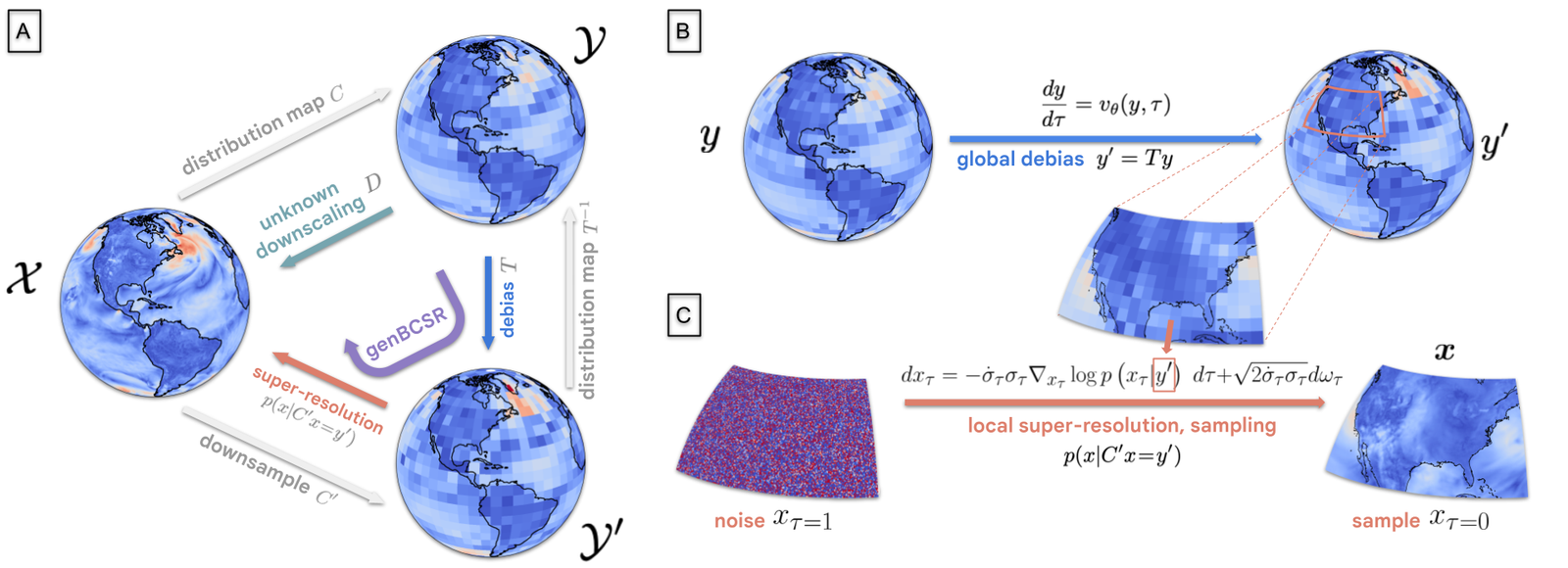
In this work, we introduce GenBCSR, Generative Bias Correction and Super-Resolution, a framework for statistical downscaling that induces a factorization of two tasks: bias correction (or debiasing) and super-resolution (or upsampling), which are instantiated using state-of-the-art generative models and applied to a challenging downscaling problem.
The bias correction step is reduced to the alignment of two distribution manifolds: the weather manifold and the climate simulation manifold. These manifolds stem from the dissipative nature of the underlying dynamical systems, which induces the data distribution to concentrate on a relatively low-dimensional manifold. The alignment is achieved using a rectified flow approach [43] that approximately solves an optimal transport problem [44], which preserves the marginals of each manifold. As such, the alignment depends on the upstream physics of the climate model, as it dictates the underlying structure of the climate simulation manifold.
The super-resolution step is a purely statistical task that relies in learning local correlations in the weather data. As such, it is completely decoupled from the climate physics modeling and it is performed only on the weather manifold, for which, we employ a probabilistic diffusion model [45] coupled with a domain decomposition technique [46] to perform regional upsampling in both space and time, obtaining arbitrarily long time-coherent samples.
We showcase our methodology by downscaling an ensemble of coarse climate simulations [47] to high-resolution local weather sequences. Even when using a handful of climate trajectories for training, we show that our strategy is able to accurately capture statistics for the full ensemble. We also show that our methodology vastly outperforms the popular BCSD method, even when the latter is trained using the full ensemble, at capturing inter-variable and spatiotemporal correlations necessary for compound events such as heat-streaks and cyclones, while remaining competitive at capturing pointwise statistics.
2 Methods
As statistical downscaling is designed to address probabilistic questions, it focuses on distributions rather than individual trajectories. Typically, this involves processing an ensemble of climate trajectories, whose snapshots are subsequently downscaled to the desired resolution.
We formulate the statistical downscaling problem by considering two stochastic processes, and with , representing a high-resolution weather process and low-resolution simulated climate process [48] respectively, governed by
| (1) | ||||
| (2) |
where embodies the generally unknown high-fidelity dynamics of , and the dynamics of are often parameterized by a stochastically forced GCM [49], in which the form of is a modelling choice. Each stochastic process333For simplicity in exposition, we follow [49] where the important time-varying effects of the seasonal and diurnal cycles have been ignored, along with jump process contributions. is associated with a time-dependent measure, and , such that and , each governed by their corresponding Fokker-Planck equations. We assume a time-invariant unknown statistical model that relates and via a possibly nonlinear downsampling map. For brevity, we omit the time-dependency of the random variables and in subsequent discussion.
In general, (2) is calibrated via measurement functionals to (1) using a single observed trajectory: the historical weather. The goal of statistical downscaling is to approximate the inverse of with a downscaling map , trained on data for , for a finite horizon , such that for . Here, denotes the push-forward measure of through , and is assumed to be time-independent.
Setup
Given its probabilistic nature, we reformulate the task of finding as sampling from a conditional distribution [50]. We define the operator , where is the identity map, such that , where is the underlying unknown joint distribution. Assuming this joint distribution admits a conditional decomposition, we have:
| (3) |
where is time-independent. Thus, we recast statistical downscaling as learning to sample from , which allows us to compute statistics of interest of via Monte-Carlo methods. A cornerstone of our approach is leveraging the map to compute this conditional probability: given a low-resolution realization , we rewrite as the conditional probability distribution .
Finally, as is assumed time-independent we model the elements and as random variables with marginal distributions, and where and . Thus, our objective is to sample given only access to marginal samples of and .
Main idea
In general, downscaling is an ill-posed problem as is unknown. Therefore, we seek to approximate so the statistical properties of are preserved given samples of . In particular, such a map should satisfy . Thus, following [41], we impose a structured ansatz to approximate by factorizing it as the composition of a known, non-invertible downsampling map444Here we suppose that the downsampling map acts both in space and in time, by using interpolation in space, and by averaging in time using a window of one day. and an invertible debiasing map :
| (4) |
or alternatively, . This factorization explicitly decouples the two objectives of downscaling: debiasing and upsampling.
The range of defines an intermediate space of debiased/low-resolution samples with measure (see Fig. 1). The joint space is built by projecting samples of into , i.e., ; see Fig. 1(a). Using these spaces, we decompose the statistical downscaling problem into the following two sub-problems:
Generative methods
In this paper we leverage two state-of-the-art generative AI techniques to build the bias correction and super-resolution maps: the bias correction step is instantiated by a conditional flow matching method [43], whereas the super-resolution step is instantiated by a conditional denoising diffusion model [51] coupled with a domain decomposition strategy [46] to upsample both in space and time and create time-coherent sequences.
Bias correction
For debiasing, we leverage manifold alignment, which arises in many applications, such as domain adaptation [52], where it seeks to generalize models by matching the training and testing distributions, particularly when they are concentrated in low-dimensional manifolds. The debiasing map T, which aligns both the climate and weather manifolds (for a visualization see S7.2), also needs to preserve large features of the input, while correcting its statistical properties. Thus, colloquially, the transformation should not "move" too much mass with respect to the input .
This notion has a long story in applied mathematics going back to Gaspar Monge in the late 1700s and Leonid Kantorovich in the 50s, who formalized this idea, and kicked off the field of optimal transport [44]. Optimal transport seeks to solve the problem
| (5) |
for a cost function , which we assume to be the Euclidean distance. Note that by construction, the debiasing map satisfies the required constraints.
Due to limitations of existing methods for solving (5) (which are briefly summarized in S1.1), we adopt a rectified flow approach [43], a methodology under the umbrella of generative models. Rectified flow solves an optimal transport problem, and it has empirically shown to generalize well while being able scale to large dimensions.
Thus we define the map as the resolvent of a ODE given by
| (6) |
whose vector field is parametrized by a neural network (see S2.1.1 for further details). By identifying the input of the map as the initial condition, we have that .
We train by solving
| (7) |
where , and is the set of couplings with marginals given by (4). The choice of the coupling is essential to obtain a correct mapping as most of the physical information, such as seasonality, is encoded in this coupling. Once the model is trained, we solve (6) using an adaptive Runge-Kutta solver. One of the main advantages of this approach relies on the fact that trajectories of smooth autonomous systems555The system in (6) is not technically autonomous, but a simple change of variables to can produce an equivalent autonomous system. can not intersect, thus as the input distribution shifts due the climate change signal, the push-forward to also needs to shift to avoid intersecting trajectories. This is an important property to preserve and we demonstrate later in Figure 5.
Super-resolution
Following alignment, the resulting samples are super-resolved in space and in time to reconstruct extended trajectories. Due to the statistical nature of this task, we leverage a conditional diffusion model, given its ability to capture underlying distributions, which is vital due to the potentially large super-resolution factor. However, this process introduces two significant challenges: i) the presence of distribution shifts in the climate projection statistics, which we aim to preserve, and ii) computational resource constraints, which require the trajectories to be processes in batches, impacting its temporal coherence.
To avoid pollution stemming from color shifts [53], due to the inherent distribution shifts in our downstream tasks, we further decompose the upsampling stage in two steps: a linear step, corresponding to cubic interpolation, and a generative step that samples the conditional residual between the original sample and its interpolation. This procedure increases robustness to distribution shifts, as the interpolation is equivariant to shifts in the mean [29].
We denote the low-resolution debiased short sequence stemming from applying to a sequence of adjacent snapshots. Following Figure 1 the upsampling stage requires sampling from , where is the high-resolution spatio-temporal sequence, is the downsampling operator, which downsamples (by interpolation plus a spectral cut-off) in space and computes daily averages in time. We define as a linear deterministic upsampling map666In principle this step can be instantiate by any deterministic upsampling map., which spatially interpolates and replicates the result across the time dimension. Then, if we define the residual as we can recast the super-resolution step as sampling from
| (8) |
This expression is instantiated by a conditional diffusion model [51] which is trained in very short trajectories pairs . This allows to define the paired residual . During training, we learn a denoiser by optimizing
| (9) |
where is a training distribution for the noise levels . predicts the clean sample of the residual given a noisy sample [54]. More details on the diffusion model formulation and training are included in S2.2.1. The learned becomes part of the sampling SDE where for a fixed coarse input , we sample the residual by solving
| (10) |
backwards in diffusion time from to with terminal condition , where is the noise schedule.
To generate long time-coherent sequences we leverage the mathematical underpinnings of sampling with diffusion models, which is reduced to solving a reverse underdamped Langevin SDE along an artificial diffusion time. As such, the temporal component of the samples becomes just another dimension, thus rendering it amenable to domain decomposition techniques, as the ones used in video generation [46].The sample generation is decomposed along the time axis in overlapping domains, at each time step each domain is advanced in diffusion time, and continuity is imposed in the overlapping regions, with an appropriate correction on the statistics of the noise, which ultimately results in time-coherent samples of arbitrary length. Further details can be found in S2.2.4.
3 Results
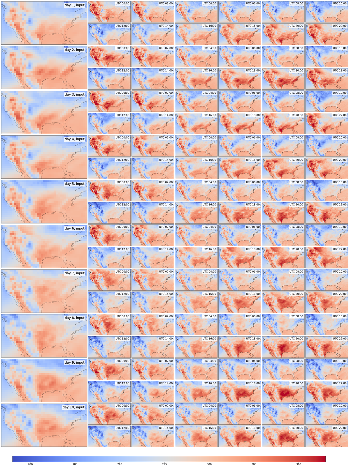
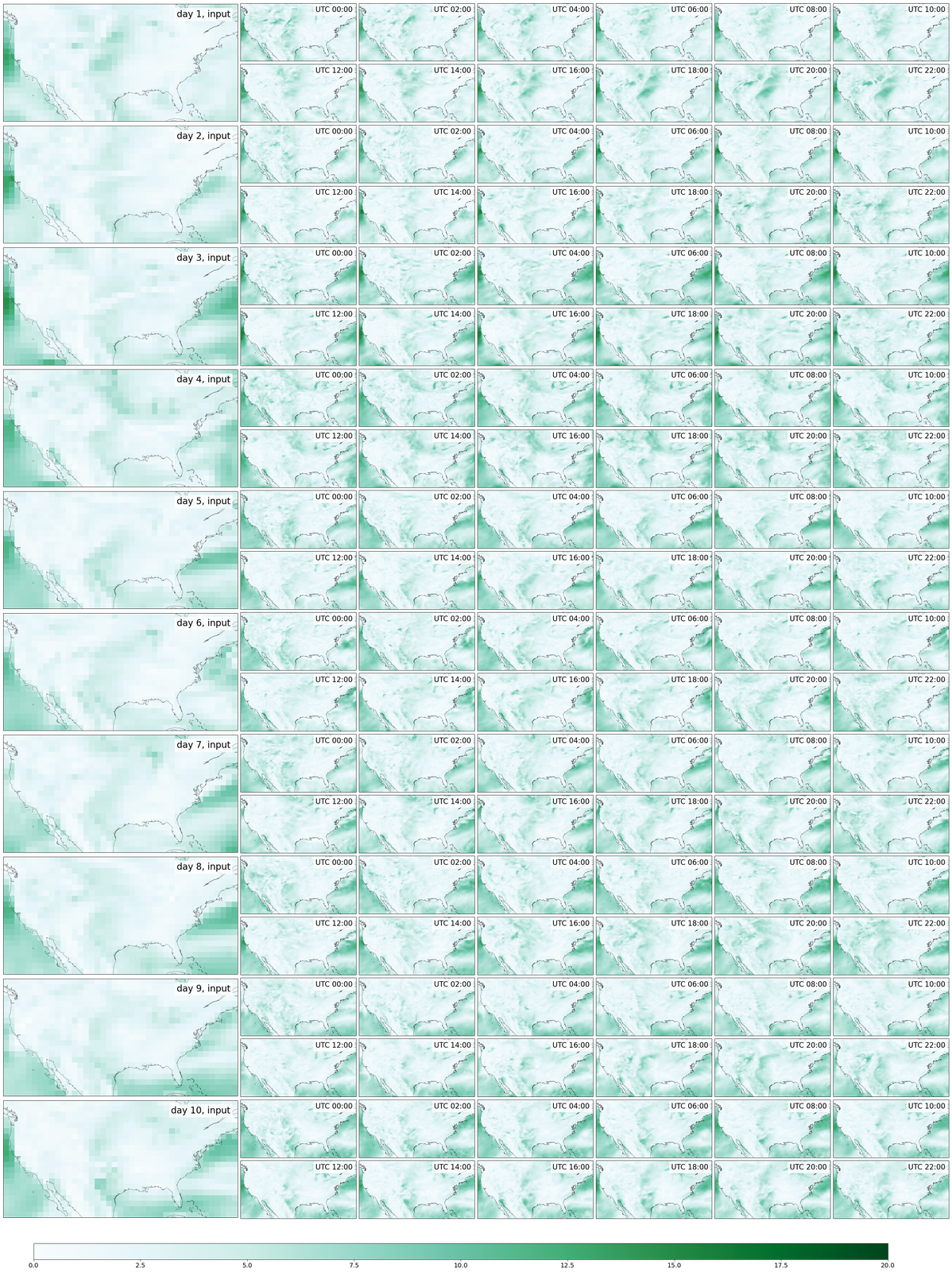
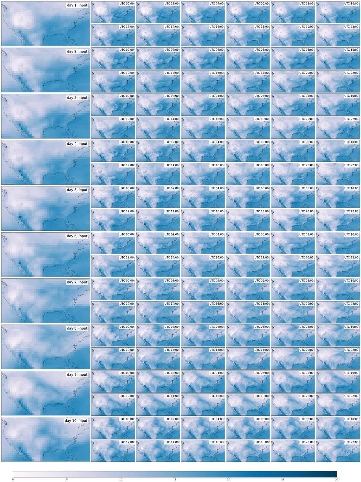
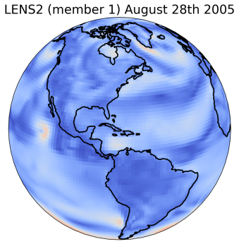
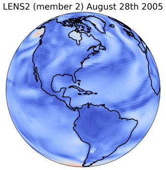
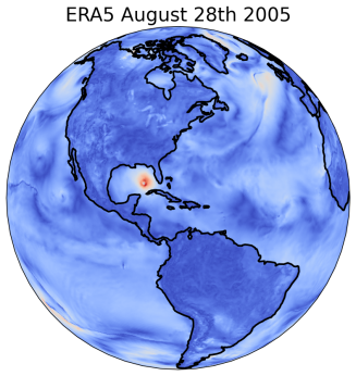
We illustrate the performance of our proposed method on a real-world, large-scale downscaling task. The coarse-resolution input is derived from the 100-member ensemble produced by the CESM2 Large Ensemble Community Project (LENS2) [47], regridded to a 1.5-degree (150 km) spatial resolution and daily averaged. Our objective is to statistically downscale key surface variables, including temperature, wind speed, humidity and sea-level pressure, to match the finer spatial-temporal characteristics of corresponding variables in the ERA5 reanalysis dataset [31], with a target resolution of 0.25-degree (25 km) in space and bi-hourly in time. This results in increasing the total resolution by a factor of 432 (). The bias correction step is applied globally, followed by regional super-resolution within a domain enclosing the Conterminous United States (CONUS)777Our approach is not region-specific. We have included results for other regions in S6.. We train the debiasing stage using as input data from 4 LENS2 ensemble members covering the period 1959-2000, and as target ERA5 reanalysis data for the same period, regridded to the LENS2 spatial-temporal resolution. Model selection and validation is performed against data from the entire LENS2 ensemble covering 2001 to 2010. The upsampling stage is trained by pairing the coarse-grained ERA5 data to its native resolution bi-hourly version. We present results for the test period from 2011 to 2020, by comparing various statistics against ERA5 observations during the same period. To prevent the results from being dominated by seasonal cycles, which have overwhelming effects on the total variations, we concentrate our evaluation on the month of August across all years.
Baselines.
We compare results from GenBCSR to output from the bias correction and spatial disaggregation (BCSD) method, a widely used statistical climate downscaling technique [55, 56, 57] (detailed in S2.3.1). BCSD employs quantile mapping (QM) between biased coarse-resolution inputs and an unbiased high-resolution reference climatology to correct biases and enhance spatial resolution, followed by a temporal disaggregation step using weighted analogs. Despite its widespread use, BCSD has notable limitations [58]. It cannot capture multivariate dependencies, often resulting in inconsistencies between related variables, and it struggles to accurately represent extreme events such as cyclones or heatwaves. These shortcomings are largely addressed by GenBCSR, as supported by the evidence presented below.
To assess the impact of the debiasing step, we also examine two alternative configurations of GenBCSR: one combining the QM-based debiasing step with generative super-resolution (QMSR) and another applying generative super-resolution directly to the original LENS2 trajectories without debiasing (SR).
Consistent representations of multi-scale variability.
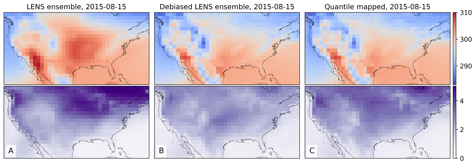
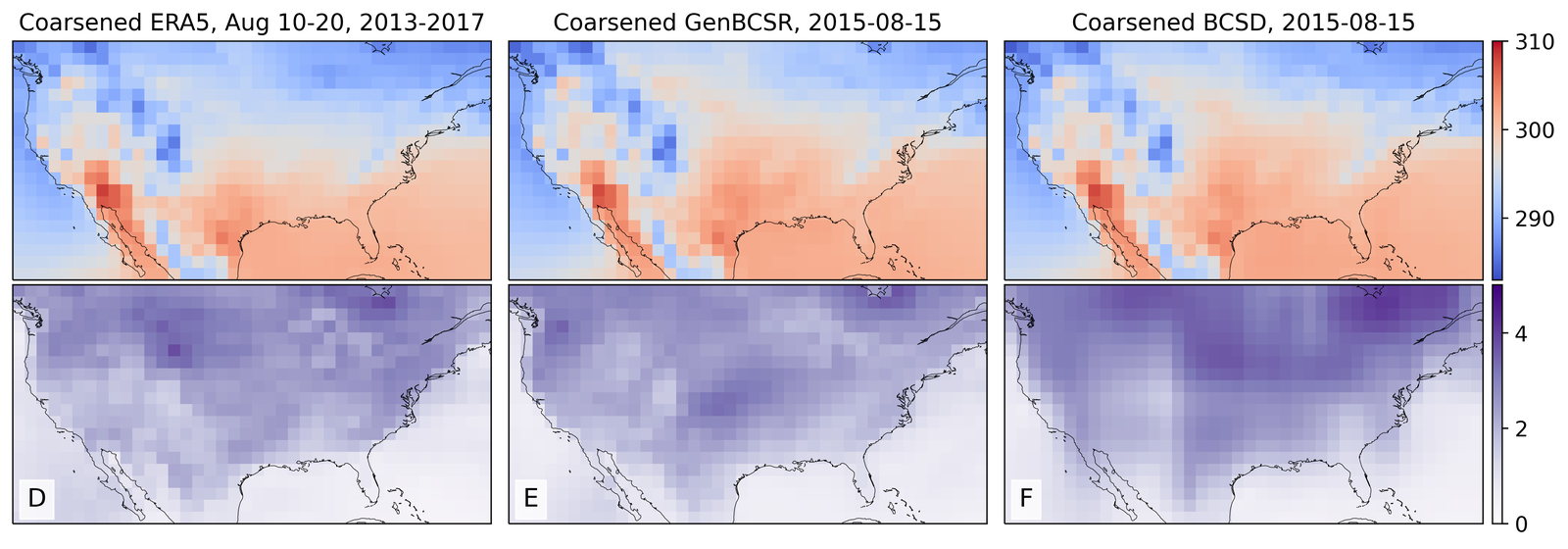
As shown in Figure 2, GenBCSR achieves consistency with large-scale inputs while introducing realistic fine-scale variability. In the debiasing step, GenBCSR modifies the original inputs (A) to better align with coarsened ERA5 observations (D). During the super-resolution step, GenBCSR (E) preserves the large-scale conditioning (B) more effectively than BCSD (F), which displays noticeable deviations from its inputs (C). Additionally, GenBCSR introduces small-scale variability, capturing spatial, diurnal, and systematic uncertainty components (S7.3). This balance between large-scale consistency and fine-scale detail highlights GenBCSR’s strength in producing reliable multi-scale downscaling results.
Effective debiasing leads to accurate inter-variable correlations and tail probabilities.
| Variable | Mean Absolute Bias | Wasserstein Distance | Mean Absolute Error, 99% | |||||||||
|---|---|---|---|---|---|---|---|---|---|---|---|---|
| GenBCSR | BCSD | QMSR | SR | GenBCSR | BCSD | QMSR | SR | GenBCSR | BCSD | QMSR | SR | |
| Temperature (K) | 0.74 | 0.70 | 0.65 | 2.68 | 0.79 | 0.78 | 0.76 | 2.72 | 0.88 | 1.07 | 1.02 | 3.17 |
| Wind speed (m/s) | 0.19 | 0.17 | 0.16 | 1.90 | 0.28 | 0.31 | 0.25 | 1.92 | 0.64 | 0.73 | 0.59 | 2.66 |
| Specific humidity (g/kg) | 0.49 | 0.45 | 0.46 | 1.55 | 0.55 | 0.54 | 0.52 | 1.63 | 0.56 | 0.81 | 0.69 | 1.77 |
| Sea-level pressure (Pa) | 68.28 | 64.13 | 63.47 | 184.53 | 67.46 | 66.92 | 65.40 | 189.23 | 97.31 | 133.29 | 111.01 | 276.87 |
| Relative humidity (%) | 2.89 | 3.21 | 3.10 | 9.35 | 3.12 | 4.43 | 3.43 | 9.52 | 3.05 | 14.00 | 4.07 | 8.16 |
| Heat index (K) | 0.58 | 0.75 | 0.72 | 2.54 | 0.64 | 0.89 | 0.77 | 2.59 | 1.35 | 1.77 | 1.50 | 4.02 |
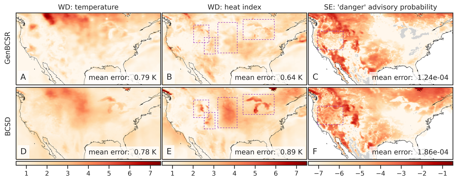
As shown in Table 1 and Figure 3, GenBCSR demonstrates strong performance in matching local pointwise marginal distributions, with mean absolute bias (MAB) capturing first-moment errors and Wasserstein distance (WD) providing a comprehensive measure of distribution discrepancies. Besides the four modeled variables, we evaluate two additional derived variables: relative humidity and heat index (S4.1). GenBCSR’s advantage over BCSD is particularly evident in these derived variables, while remaining competitive for directly predicted ones. This highlights GenBCSR’s superior ability to capture inter-variable correlations while accurately aligning marginal distributions. The improvements are most notable in regions such as the North West, Central US, and around the Great Lakes, as shown in Figure 3 (B and E).
The advantage of GenBCSR becomes more pronounced when focusing on distribution tails, which are crucial for representing extreme weather events with significant real-world consequences. Table 1 shows that GenBCSR achieves lower MAE at the 99th percentile across most variables. This strength is further illustrated in Figure 3 (C), which depicts the probability of heat advisory conditions, defined by local heat indices exceeding the “danger" threshold of 312.6 K [59] (additional levels provided in S6). Across various tail thresholds, GenBCSR consistently exhibits significantly lower errors than BCSD, underscoring its robustness in predicting high-impact extremes.
The importance of multivariate debiasing is further emphasized through comparisons against alternative configurations. While QM-based debiasing combined with generative super-resolution (QMSR) reduces errors compared to no debiasing (SR) and is very effective for directly modeled variables, it still underperforms GenBCSR for derived variables and extreme tails. In contrast, perfect debiasing dramatically reduces errors (S5.2), reinforcing the critical role of accurate debiasing in improving model performance. These comparisons demonstrate that GenBCSR’s debiasing step allows for a better characterization of inter-variable correlations and tail statistics.
Superior spatio-temporal correlations and compound event statistics.
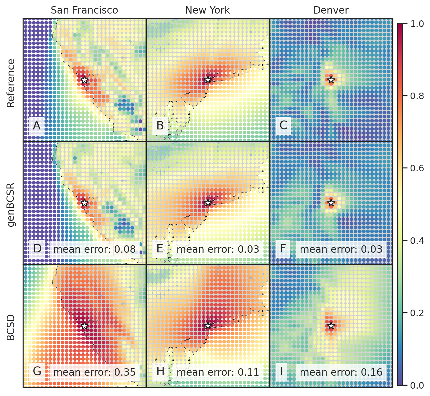
In addition to capturing inter-variable correlations, GenBCSR demonstrates significant improvements in representing spatial and temporal correlations. Figure 4 (A-I) illustrates the spatial correlation of surface wind speed at selected U.S. cities relative to nearby locations. The patterns produced by GenBCSR align closely with ERA5 observations, accurately reflecting the influence of geographic features and regional meteorology. Unlike BCSD, which produces overly smoothed correlations and misses finer regional details, GenBCSR effectively preserves local variability and resolves complex spatial structures.
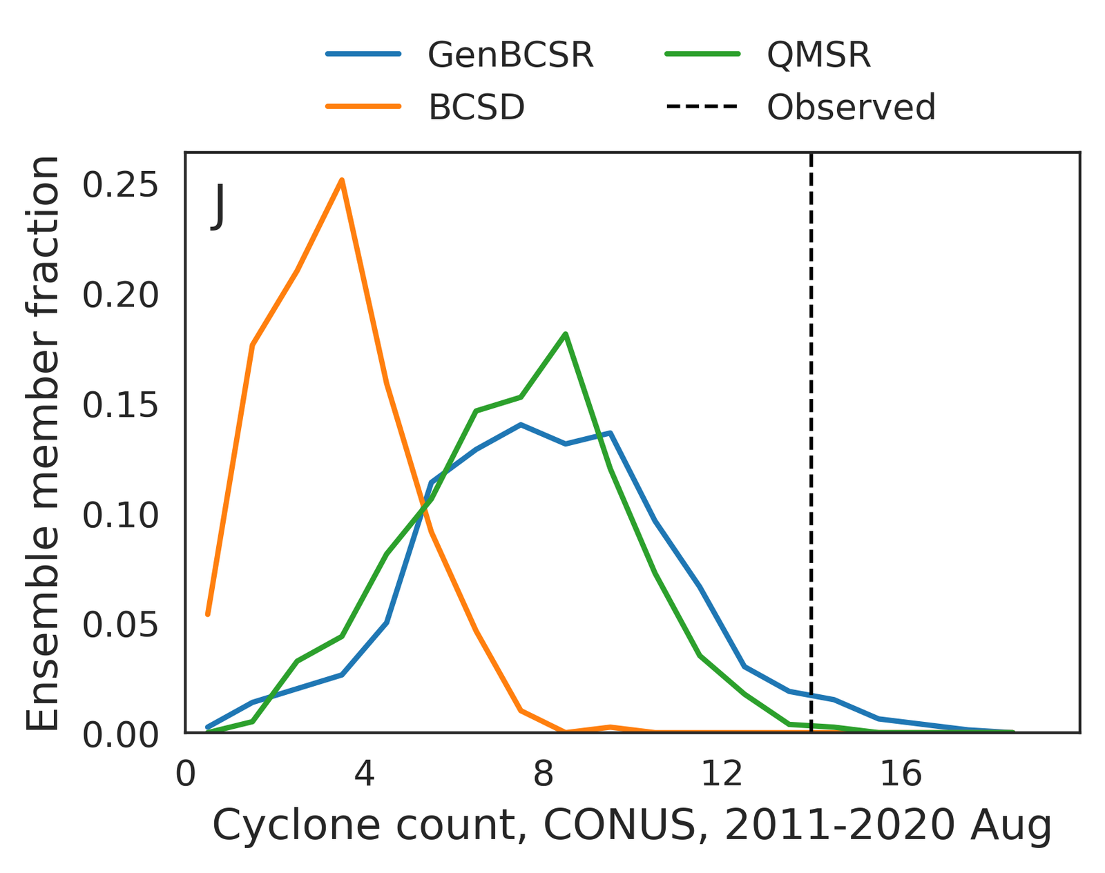
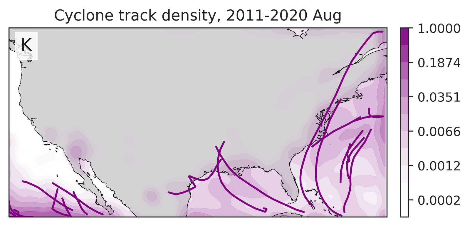
Tropical cyclones, with their pronounced spatial-temporal dependencies, serve as a representative example of GenBCSR’s proficiency in modeling compound event statistics. As shown in Figure 4 (J-K), when using TempestExtremes [103] to detect tropical cyclones, GenBCSR yields improved count statistics compared to the BCSD baseline, bringing them closer to those observed in ERA5. These improvements are largely attributed to the spatio-temporal upsampling in our approach, which, when combined with QM, also results in noticeable enhancements in the cyclone counts.
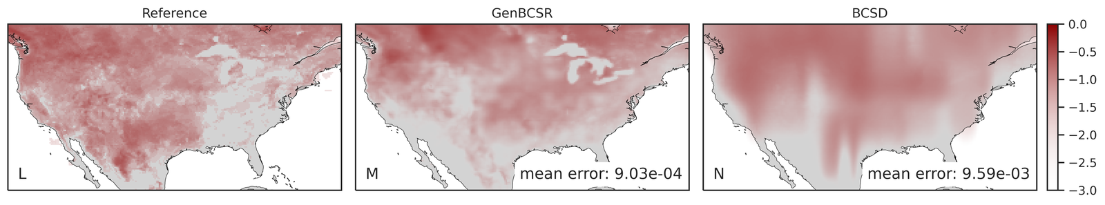
Prolonged heat streaks represent another example of compound events with significant impacts on human activities. Figure 4 (L-N) presents the predicted probabilities for heat streaks, defined as daily maximum temperatures exceeding climatology for multiple consecutive days. GenBCSR demonstrates a clear advantage over BCSD, capturing the frequency and intensity of these extreme events with significantly greater accuracy (additional results in S6). This improvement reflects GenBCSR’s ability to retain critical temporal dependencies, offering a more reliable representation of persistent extremes that are essential for understanding and adapting to climate impacts.
Robust to out-of-distribution shift due to nonstationarity
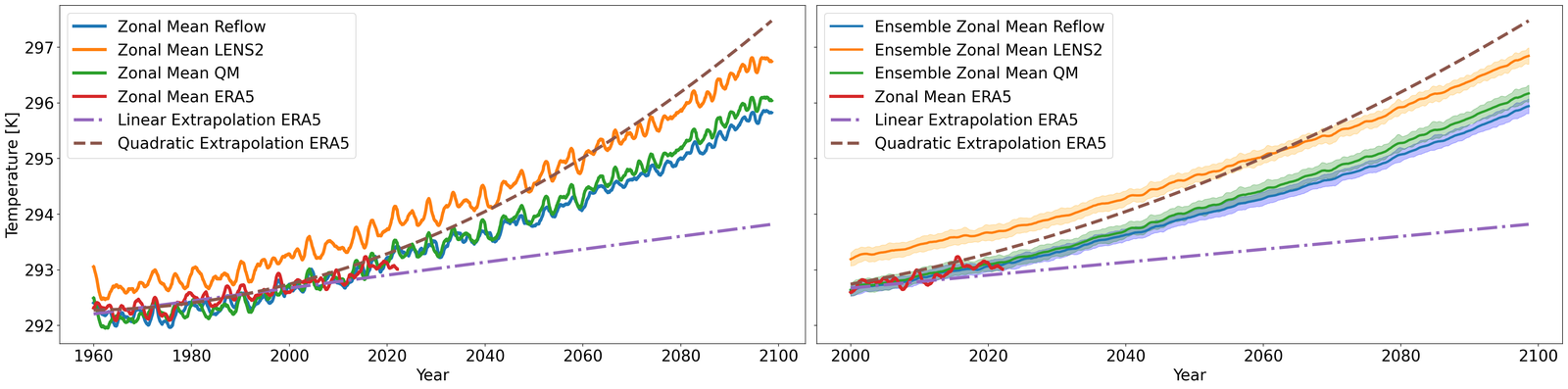
As climate is non-stationary, it is key for learning methods, optimized on past historical data, to be robust to distribution shifts. In particular, preserving climate change signals is crucial as statistical blending can erase the signal in climate projection ensembles [58]. To this end, we demonstrate that the bias-correction procedure in our method can preserve well long-term trends, attributing to learning a velocity field to remove the bias.
The results are compiled in Figure 5. There, we compute the projected zonal mean 2 meter temperatures (between °N and °S), time-averaged with a rolling window of one year (defined in S7.1.1), for the LENS2 ensemble, the bias-corrected samples (without super-resolution) using GenBCSR and QM, and the low-resolution ERA5 ground truth. In Figure 5 (left), we observe that the statistics of the debiased trajectory (from one of the ensemble members used for training) match the statistics of ERA5 for the training period (1960-2000), and then follow a similar trend to LENS2 for the next 60 years. In Figure 5(right), we observe that when debiasing the full LENS2 ensemble, the evaluation and testing statistics of ERA5 are within one standard deviation of the mean debiased statistics, which are then driven by the LENS2 statistics going forward.
It is not surprising to note that QM can also preserve the trend as it matches marginal (single-variate) distributions. However, importantly, it is worthwhile to observe that learning a high-dimensional velocity field as in equation 6 to match high-dimensional distributions is robust to the distribution shifts (after the training period). Furthermore, we note that simple linear extrapolation used from ERA5 data predicts a slower increase in zonal mean temperature, whereas a quadratic extrapolation predicts a faster increase. Viewing those two as massively simplified versions of mapping between distributions, we see the benefits of learning highly nonlinear mapping through the rectified approach equation 7, highlighting the need for preserving complex climate change signals involving multiple variables [58]. See S7.1 for extra results, including seasonal variability, and bias.
Finally, we briefly mention that this preservation of long-term trends can pass through the super-resolution stage so that the statistics in the final outputs also correlate with the trends, an important property we need to have for the method to be applicable to future climate projections. See Figure S6 in SI for details.
4 Discussion
We introduce a generative spatiotemporal statistical downscaling framework for unpaired data. Our methodology stems from a novel factorization of statistical downscaling into debiasing (or manifold alignment) and upsampling, in which each step is instantiated by a highly tailored generative model. Our approach addresses key limitations of prior methods for unpaired data, such as BCSD, by capturing both the local marginal distributions and inter-variable spatio-temporal correlations more effectively. By leveraging spatial interpolation and a diffusion-based residual generator, our model can represent fine-scale structures and temporal dynamics that are often overlooked by traditional techniques. This allows for more accurate and realistic downscaling of climate variables from coarse-resolution simulations to high-resolution outputs.
The practical implications of our method are significant, particularly for downstream applications where localized climate predictions are critical and paired data is not available. For instance, accurate spatial correlation modeling can improve renewable energy planning by better forecasting wind patterns for optimized wind farm placement, along with better spatial correlation of the heat index for improved electrical grid planning, especially for high-voltage power lines [20]. Additionally, the ability to capture inter-variable correlations, such as those between temperature and humidity, is essential for predicting the heat index, which has direct applications in public health, food production [17], energy demand forecasting [19, 20], and disaster preparedness [5]. Furthermore, our model’s improved temporal correlations enhance the ability to predict extreme events, such as prolonged heat waves, with significantly greater accuracy than BCSD, offering more reliable insights for managing heat-related risks [60, 61].
Looking forward, the current approach opens up several opportunities for further methodological development. One promising direction is the integration of additional auxiliary datasets, such as satellite-derived data or local observational networks, to improve the model’s robustness in regions with sparse data. Another direction is downscale data from an ensemble of climate models as we only require unpaired data and only the bias correction step relies on the physics of the climate models, thus providing localized forecasts capturing not only the internal variability of each model, but also the variability across different climate models. These developments have the potential to further refine the downscaling of climate simulations, making the method applicable to a broader range of variables, climate models, and geographic regions. Ultimately, this work contributes to the growing body of research on improving the resolution and accuracy of climate predictions, with far-reaching impacts in fields such as climate change mitigation, resource management, and environmental risk assessment.
Acknowledgement
We thank Lizao Li and Stephan Hoyer for productive discussions and Daniel Worrall for feedback on the manuscript. For the LENS2 dataset, we acknowledge the CESM2 Large Ensemble Community Project and the supercomputing resources provided by the IBS Center for Climate Physics in South Korea. ERA5 data [62] were downloaded from the Copernicus Climate Change Service [63]. The results contain modified Copernicus Climate Change Service information. Neither the European Commission nor ECMWF is responsible for any use that may be made of the Copernicus information or data it contains. We thank Tyler Russell for managing data acquisition and other internal business processes.
References
- \bibcommenthead
- [1] Balaji, V. et al. Are general circulation models obsolete? Proceedings of the National Academy of Sciences 119, e2202075119 (2022). URL https://www.pnas.org/doi/abs/10.1073/pnas.2202075119.
- [2] Courant, R., Friedrichs, K. & Lewy, H. Über die partiellen differenzengleichungen der mathematischen physik. Mathematische annalen 100, 32–74 (1928).
- [3] Schneider, T. et al. Climate goals and computing the future of clouds. Nature Climate Change 7, 3–5 (2017).
- [4] Knutson, T. R. et al. Dynamical downscaling projections of twenty-first-century Atlantic hurricane activity: CMIP3 and CMIP5 model-based scenarios. Journal of Climate 26, 6591–6617 (2013).
- [5] Goss, M. et al. Climate change is increasing the likelihood of extreme autumn wildfire conditions across California. Environmental Research Letters 15, 094016 (2020).
- [6] Christensen, J. H., Boberg, F., Christensen, O. B. & Lucas-Picher, P. On the need for bias correction of regional climate change projections of temperature and precipitation. Geophysical Research Letters 35 (2008). URL https://agupubs.onlinelibrary.wiley.com/doi/abs/10.1029/2008GL035694.
- [7] Zelinka, M. D. et al. Causes of higher climate sensitivity in cmip6 models. Geophysical Research Letters 47, e2019GL085782 (2020). URL https://agupubs.onlinelibrary.wiley.com/doi/abs/10.1029/2019GL085782. E2019GL085782 10.1029/2019GL085782.
- [8] Pepin, N. et al. Elevation-dependent warming in mountain regions of the world. Nature Climate Change 5, 424–430 (2015).
- [9] Grotch, S. L. & MacCracken, M. C. The use of general circulation models to predict regional climatic change. Journal of Climate 4, 286 – 303 (1991). URL https://journals.ametsoc.org/view/journals/clim/4/3/1520-0442_1991_004_0286_tuogcm_2_0_co_2.xml.
- [10] Hall, A. Projecting regional change. Science 346, 1461–1462 (2014). URL https://www.science.org/doi/abs/10.1126/science.aaa0629.
- [11] Diffenbaugh, N. S., Pal, J. S., Trapp, R. J. & Giorgi, F. Fine-scale processes regulate the response of extreme events to global climate change. Proceedings of the National Academy of Sciences 102, 15774–15778 (2005).
- [12] Gutowski, W. J. et al. The ongoing need for high-resolution regional climate models: Process understanding and stakeholder information. Bulletin of the American Meteorological Society 101, E664–E683 (2020).
- [13] Gutmann, E. et al. An intercomparison of statistical downscaling methods used for water resource assessments in the united states. Water Resources Research 50, 7167–7186 (2014). URL https://agupubs.onlinelibrary.wiley.com/doi/abs/10.1002/2014WR015559.
- [14] Hwang, S. & Graham, W. D. Assessment of alternative methods for statistically downscaling daily gcm precipitation outputs to simulate regional streamflow. JAWRA Journal of the American Water Resources Association 50, 1010–1032 (2014). URL https://onlinelibrary.wiley.com/doi/abs/10.1111/jawr.12154.
- [15] Naveena, N. et al. Statistical downscaling in maximum temperature future climatology. AIP Conference Proceedings 2357 (2022). URL https://doi.org/10.1063/5.0081087. 030026.
- [16] Abatzoglou, J. T. & Brown, T. J. A comparison of statistical downscaling methods suited for wildfire applications. International Journal of Climatology 32, 772–780 (2012). URL https://rmets.onlinelibrary.wiley.com/doi/abs/10.1002/joc.2312.
- [17] Wang, B. et al. Sources of uncertainty for wheat yield projections under future climate are site-specific. Nature Food 1, 720–728 (2020).
- [18] Teutschbein, C. & Seibert, J. Bias correction of regional climate model simulations for hydrological climate-change impact studies: Review and evaluation of different methods. Journal of Hydrology 456-457, 12–29 (2012).
- [19] Damiani, A., Ishizaki, N. N., Sasaki, H., Feron, S. & Cordero, R. R. Exploring super-resolution spatial downscaling of several meteorological variables and potential applications for photovoltaic power. Scientific Reports 14, 7254 (2024).
- [20] Dumas, M., Kc, B. & Cunliff, C. I. Extreme weather and climate vulnerabilities of the electric grid: A summary of environmental sensitivity quantification methods. Tech. Rep., Oak Ridge National Lab.(ORNL), Oak Ridge, TN (United States) (2019).
- [21] Wilby, R. L. et al. Statistical downscaling of general circulation model output: A comparison of methods. Water Resources Research 34, 2995–3008 (1998). URL https://agupubs.onlinelibrary.wiley.com/doi/abs/10.1029/98WR02577.
- [22] Wilby, R. L. et al. Integrated modelling of climate change impacts on water resources and quality in a lowland catchment: River kennet, uk. J. Hydrol. 330, 204–220 (2006).
- [23] Bischoff, T. & Deck, K. Unpaired downscaling of fluid flows with diffusion bridges. Artificial Intelligence for the Earth Systems 3, e230039 (2024).
- [24] Hammoud, M. A. E. R., Titi, E. S., Hoteit, I. & Knio, O. Cdanet: A physics-informed deep neural network for downscaling fluid flows. Journal of Advances in Modeling Earth Systems 14, e2022MS003051 (2022).
- [25] Harris, L., McRae, A. T., Chantry, M., Dueben, P. D. & Palmer, T. N. A generative deep learning approach to stochastic downscaling of precipitation forecasts. Journal of Advances in Modeling Earth Systems 14, e2022MS003120 (2022).
- [26] Price, I. & Rasp, S. Increasing the accuracy and resolution of precipitation forecasts using deep generative models, 10555–10571 (PMLR, 2022).
- [27] Harder, P. et al. Generating physically-consistent high-resolution climate data with hard-constrained neural networks. arXiv preprint arXiv:2208.05424 (2022).
- [28] Mardani, M. et al. Residual corrective diffusion modeling for km-scale atmospheric downscaling. arXiv preprint arXiv:2309.15214 (2023).
- [29] Lopez-Gomez, I. et al. Dynamical-generative downscaling of climate model ensembles. arXiv preprint arXiv:2410.01776 (2024).
- [30] Danabasoglu, G. et al. The community earth system model version 2 (cesm2). Journal of Advances in Modeling Earth Systems 12, e2019MS001916 (2020). URL https://agupubs.onlinelibrary.wiley.com/doi/abs/10.1029/2019MS001916. E2019MS001916 2019MS001916.
- [31] Hersbach, H. et al. The ERA5 global reanalysis. Quarterly Journal of the Royal Meteorological Society 146, 1999–2049 (2020). URL https://rmets.onlinelibrary.wiley.com/doi/abs/10.1002/qj.3803.
- [32] Dixon, K. W. et al. Evaluating the stationarity assumption in statistically downscaled climate projections: is past performance an indicator of future results? Climatic Change 135, 395–408 (2016).
- [33] Huang, X., Swain, D. L. & Hall, A. D. Future precipitation increase from very high resolution ensemble downscaling of extreme atmospheric river storms in california. Science Advances 6, eaba1323 (2020). URL https://www.science.org/doi/abs/10.1126/sciadv.aba1323.
- [34] Doblas-Reyes, F. et al. Linking Global to Regional Climate Change., 1363–1512 (Cambridge University Press, Cambridge, United Kingdom, 2021).
- [35] Pan, B. et al. Learning to correct climate projection biases. Journal of Advances in Modeling Earth Systems 13, e2021MS002509 (2021).
- [36] Dong, C., Loy, C. C., He, K. & Tang, X. Fleet, D., Pajdla, T., Schiele, B. & Tuytelaars, T. (eds) Learning a deep convolutional network for image super-resolution. (eds Fleet, D., Pajdla, T., Schiele, B. & Tuytelaars, T.) Computer Vision – ECCV 2014, 184–199 (Springer International Publishing, Cham, 2014).
- [37] Cheng, J. et al. Reslap: Generating high-resolution climate prediction through image super-resolution. IEEE Access 8, 39623–39634 (2020).
- [38] Vandal, T. et al. DeepSD: Generating high resolution climate change projections through single image super-resolution, KDD ’17, 1663–1672 (Association for Computing Machinery, New York, NY, USA, 2017). URL https://doi.org/10.1145/3097983.3098004.
- [39] Candès, E. J. & Fernandez-Granda, C. Towards a mathematical theory of super-resolution. Communications on Pure and Applied Mathematics 67, 906–956 (2014). URL https://onlinelibrary.wiley.com/doi/abs/10.1002/cpa.21455.
- [40] Kolmogorov, A. N. A refinement of previous hypotheses concerning the local structure of turbulence in a viscous incompressible fluid at high reynolds number. Journal of Fluid Mechanics 13, 82–85 (1962).
- [41] Wan, Z. Y. et al. Debias coarsely, sample conditionally: Statistical downscaling through optimal transport and probabilistic diffusion models. Advances in Neural Information Processing Systems 36, 47749–47763 (2023).
- [42] Mémoli, F. Gromov–wasserstein distances and the metric approach to object matching. Foundations of computational mathematics 11, 417–487 (2011).
- [43] Liu, X., Gong, C. & Liu, Q. Flow straight and fast: Learning to generate and transfer data with rectified flow (2023). URL https://openreview.net/forum?id=XVjTT1nw5z.
- [44] Villani, C. Optimal transport: old and new (Springer Berlin Heidelberg, 2009).
- [45] Karras, T., Aittala, M., Aila, T. & Laine, S. Elucidating the design space of diffusion-based generative models. Advances in neural information processing systems 35, 26565–26577 (2022).
- [46] Bar-Tal, O. et al. Lumiere: A space-time diffusion model for video generation. arXiv preprint arXiv:2401.12945 (2024).
- [47] Rodgers, K. B. et al. Ubiquity of human-induced changes in climate variability. Earth System Dynamics 12, 1393–1411 (2021). URL https://esd.copernicus.org/articles/12/1393/2021/.
- [48] Majda, A. J. Challenges in climate science and contemporary applied mathematics. Communications on Pure and Applied Mathematics 65, 920–948 (2012).
- [49] O’Neill, B. C. et al. The scenario model intercomparison project (ScenarioMIP) for CMIP6. Geoscientific Model Development 9, 3461–3482 (2016).
- [50] Molinaro, R. et al. Generative AI for fast and accurate statistical computation of fluids. arXiv preprint arXiv:2409.18359 (2024).
- [51] Song, Y. & Ermon, S. Improved techniques for training score-based generative models. Advances in neural information processing systems 33, 12438–12448 (2020).
- [52] Gong, B., Shi, Y., Sha, F. & Grauman, K. Geodesic flow kernel for unsupervised domain adaptation, 2066–2073 (IEEE, 2012).
- [53] Deck, K. & Bischoff, T. Easing color shifts in score-based diffusion models. arXiv preprint arXiv:2306.15832 (2023).
- [54] Song, Y. et al. Score-based generative modeling through stochastic differential equations. CoRR abs/2011.13456 (2020). URL https://arxiv.org/abs/2011.13456.
- [55] Wood, A. W., Maurer, E. P., Kumar, A. & Lettenmaier, D. P. Long-range experimental hydrologic forecasting for the eastern united states. Journal of Geophysical Research: Atmospheres 107, ACL–6 (2002).
- [56] Wood, A. W., Leung, L. R., Sridhar, V. & Lettenmaier, D. Hydrologic implications of dynamical and statistical approaches to downscaling climate model outputs. Climatic change 62, 189–216 (2004).
- [57] Thrasher, B., Maurer, E. P., McKellar, C. & Duffy, P. B. Technical note: Bias correcting climate model simulated daily temperature extremes with quantile mapping. Hydrology and Earth System Sciences 16, 3309–3314 (2012).
- [58] Chandel, V. S., Bhatia, U., Ganguly, A. R. & Ghosh, S. State-of-the-art bias correction of climate models misrepresent climate science and misinform adaptation. Environmental Research Letters 19, 094052 (2024).
- [59] National Oceanic and Atmospheric Administration (NOAA). Heat forecast tools. URL https://www.weather.gov/safety/heat-index.
- [60] Delworth, T. L., Mahlman, J. D. & Knutson, T. R. Changes in heat index associated with CO2-induced global warming. Climatic change 43, 369–386 (1999).
- [61] Dahl, K., Licker, R., Abatzoglou, J. T. & Declet-Barreto, J. Increased frequency of and population exposure to extreme heat index days in the united states during the 21st century. Environmental research communications 1, 075002 (2019).
- [62] Hersbach, H. et al. ERA5 hourly data on single levels from 1940 to present (2023).
- [63] Copernicus Climate Change Service, Climate Data Store. ERA5 hourly data on single levels from 1940 to present (2023).
- [64] Charalampopoulos, A.-T., Zhang, S., Harrop, B., Leung, L.-y. R. & Sapsis, T. Statistics of extreme events in coarse-scale climate simulations via machine learning correction operators trained on nudged datasets. arXiv preprint arXiv:2304.02117 (2023).
- [65] Candès, E. J. & Fernandez-Granda, C. Super-resolution from noisy data. Journal of Fourier Analysis and Applications 19, 1229–1254 (2013). URL https://doi.org/10.1007/s00041-013-9292-3.
- [66] Hua, Y. & Sarkar, T. K. On SVD for estimating generalized eigenvalues of singular matrix pencil in noise. IEEE Trans. Sig. Proc. 39, 892–900 (1991).
- [67] Roy, R. & Kailath, T. ESPRIT-estimation of signal parameters via rotational invariance techniques. IEEE Transactions on acoustics, speech, and signal processing 37, 984–995 (1989).
- [68] Schmidt, R. Multiple emitter location and signal parameter estimation. IEEE transactions on antennas and propagation 34, 276–280 (1986).
- [69] Vandal, T., Kodra, E. & Ganguly, A. R. Intercomparison of machine learning methods for statistical downscaling: the case of daily and extreme precipitation. Theoretical and Applied Climatology 137, 557–570 (2019).
- [70] Maraun, D. Bias correction, quantile mapping, and downscaling: Revisiting the inflation issue. Journal of Climate 26, 2137 – 2143 (2013). URL https://journals.ametsoc.org/view/journals/clim/26/6/jcli-d-12-00821.1.xml.
- [71] Hessami, M., Gachon, P., Ouarda, T. B. & St-Hilaire, A. Automated regression-based statistical downscaling tool. Environmental Modelling and Software 23, 813–834 (2008). URL https://www.sciencedirect.com/science/article/pii/S1364815207001867.
- [72] Bortoli, V. D., Thornton, J., Heng, J. & Doucet, A. Beygelzimer, A., Dauphin, Y., Liang, P. & Vaughan, J. W. (eds) Diffusion schrödinger bridge with applications to score-based generative modeling. (eds Beygelzimer, A., Dauphin, Y., Liang, P. & Vaughan, J. W.) Advances in Neural Information Processing Systems (2021). URL https://openreview.net/forum?id=9BnCwiXB0ty.
- [73] Choi, J., Kim, S., Jeong, Y., Gwon, Y. & Yoon, S. Ilvr: Conditioning method for denoising diffusion probabilistic models. arXiv preprint arXiv:2108.02938 (2021).
- [74] Meng, C. et al. SDEdit: Guided image synthesis and editing with stochastic differential equations (2021).
- [75] Park, T., Efros, A. A., Zhang, R. & Zhu, J.-Y. Contrastive learning for unpaired image-to-image translation, 319–345 (Springer, 2020).
- [76] Sasaki, H., Willcocks, C. G. & Breckon, T. P. UNIT-DDPM: Unpaired image translation with denoising diffusion probabilistic models. arXiv preprint arXiv:2104.05358 (2021).
- [77] Su, X., Song, J., Meng, C. & Ermon, S. Dual diffusion implicit bridges for image-to-image translation (2023). URL https://openreview.net/forum?id=5HLoTvVGDe.
- [78] Wu, C. H. & De la Torre, F. Unifying diffusion models’ latent space, with applications to cyclediffusion and guidance. arXiv preprint arXiv:2210.05559 (2022).
- [79] Zhao, M., Bao, F., Li, C. & Zhu, J. Egsde: Unpaired image-to-image translation via energy-guided stochastic differential equations. arXiv preprint arXiv:2207.06635 (2022).
- [80] Grover, A., Chute, C., Shu, R., Cao, Z. & Ermon, S. Alignflow: Cycle consistent learning from multiple domains via normalizing flows (2019). URL https://openreview.net/forum?id=S1lNELLKuN.
- [81] Groenke, B., Madaus, L. & Monteleoni, C. Climalign: Unsupervised statistical downscaling of climate variables via normalizing flows, CI2020, 60–66 (Association for Computing Machinery, New York, NY, USA, 2021). URL https://doi.org/10.1145/3429309.3429318.
- [82] Cuturi, M. Sinkhorn distances: Lightspeed computation of optimal transport. Advances in neural information processing systems 26 (2013).
- [83] Courty, N., Flamary, R., Habrard, A. & Rakotomamonjy, A. Joint distribution optimal transportation for domain adaptation. Advances in neural information processing systems 30 (2017).
- [84] Flamary, R., Courty, N., Tuia, D. & Rakotomamonjy, A. Optimal transport for domain adaptation. IEEE Trans. Pattern Anal. Mach. Intell 1 (2016).
- [85] Papadakis, N. Optimal transport for image processing. Ph.D. thesis, Université de Bordeaux (2015).
- [86] Tian, C., Zhang, X., Lin, J. C.-W., Zuo, W. & Zhang, Y. Generative adversarial networks for image super-resolution: A survey. arXiv preprint arXiv:2204.13620 (2022).
- [87] Lugmayr, A., Danelljan, M., Van Gool, L. & Timofte, R. SRFlow: Learning the super-resolution space with normalizing flow (2020).
- [88] Dhariwal, P. & Nichol, A. Diffusion models beat gans on image synthesis. Advances in Neural Information Processing Systems 34, 8780–8794 (2021).
- [89] Li, H. et al. Srdiff: Single image super-resolution with diffusion probabilistic models. Neurocomputing 479, 47–59 (2022). URL https://www.sciencedirect.com/science/article/pii/S0925231222000522.
- [90] Finzi, M. A., Boral, A., Wilson, A. G., Sha, F. & Zepeda-Núñez, L. Krause, A. et al. (eds) User-defined event sampling and uncertainty quantification in diffusion models for physical dynamical systems. (eds Krause, A. et al.) Proceedings of the 40th International Conference on Machine Learning, Vol. 202 of Proceedings of Machine Learning Research, 10136–10152 (PMLR, 2023). URL https://proceedings.mlr.press/v202/finzi23a.html.
- [91] Amos, B., Xu, L. & Kolter, J. Z. Precup, D. & Teh, Y. W. (eds) Input convex neural networks. (eds Precup, D. & Teh, Y. W.) Proceedings of the 34th International Conference on Machine Learning, Vol. 70 of Proceedings of Machine Learning Research, 146–155 (PMLR, 2017). URL https://proceedings.mlr.press/v70/amos17b.html.
- [92] Bao, F., Li, C., Cao, Y. & Zhu, J. All are worth words: a vit backbone for score-based diffusion models (2022). URL https://openreview.net/forum?id=WfkBiPO5dsG.
- [93] Anderson, B. D. Reverse-time diffusion equation models. Stochastic Processes and their Applications 12, 313–326 (1982).
- [94] Efron, B. Tweedie’s formula and selection bias. Journal of the American Statistical Association 106, 1602–1614 (2011).
- [95] Ho, J. & Salimans, T. Classifier-free diffusion guidance (2022). URL https://arxiv.org/abs/2207.12598. 2207.12598.
- [96] Wood, A. W., Maurer, E. P., Kumar, A. & Lettenmaier, D. P. Long-range experimental hydrologic forecasting for the eastern United States. Journal of Geophysical Research: Atmospheres 107, ACL 6–1–ACL 6–15 (2002).
- [97] Danabasoglu, G. et al. The community earth system model version 2 (CESM2). Journal of Advances in Modeling Earth Systems 12, e2019MS001916 (2020).
- [98] Eyring, V. et al. Overview of the coupled model intercomparison project phase 6 (CMIP6) experimental design and organization. Geoscientific model development 9, 1937–1958 (2016).
- [99] Fasullo, J. T. et al. An overview of the E3SM version 2 large ensemble and comparison to other E3SM and CESM large ensembles. Earth system dynamics 15, 367–386 (2024).
- [100] Soci, C. et al. The ERA5 global reanalysis from 1940 to 2022. Quarterly journal of the Royal Meteorological Society. Royal Meteorological Society (Great Britain) 150, 4014–4048 (2024).
- [101] Rothfusz, L. P. The heat index “equation” (or, more than you ever wanted to know about heat index). Technical Attachment SR 90-23, NWS Southern Region Headquarters (1990).
- [102] National Weather Service. Heat index equation. https://www.wpc.ncep.noaa.gov/html/heatindex_equation.shtml. Accessed: 2024-12-08.
- [103] Ullrich, P. A. et al. Tempestextremes v2. 1: A community framework for feature detection, tracking, and analysis in large datasets. Geoscientific Model Development 14, 5023–5048 (2021).
Appendix S1 Related work
The most direct approach to super-resolve low-resolution data is to learn a low- to high-resolution mapping via paired data when it is possible to collect such data [29]. For complex dynamical systems, as the one arising from climate simulations, several methods carefully manipulate high- and low-resolution models, either by nudging or by enforcing boundary conditions, to produce paired data without introducing spectral biases [64, 32]. Alternatively, if one has strong prior knowledge about the downsampling process, optimization methods can solve an inverse problem to directly estimate the high-resolution data, leveraging prior assumptions such as sparsity in compressive sensing [65, 39] or translation invariance [66, 67, 68].
In the climate projection setting, there is no straightforward way to obtain paired data due to the nature of the problem (i.e., turbulent flows, with characteristically different statistics across a large span of spatiotemporal scales). In the weather and climate literature (see [69] for an extensive overview), prior knowledge can be exploited to downscale specific variables [21]. One of the most predominant methods of this type is bias correction and spatial disaggregation (BCSD), which combines traditional spline interpolation with a quantile matching bias correction [70] and a disaggregation step , and linear models [71]. Recently, several studies have used ML to downscale physical quantities such as precipitation [38], but without quantifying the uncertainty of the prediction. Yet, to our knowledge, a generally applicable method to downscale arbitrary variables under an assumption of unpaired data is lacking.
Another difficulty is to remove the bias in the low resolution data. This is an instance of domain adaptation, a topic popularly studied in computer vision. Recent work has used generative models such as GANs and diffusion models to bridge the gap between two domains [23, 72, 73, 74, 35, 75, 76, 77, 78, 79]. A popular domain alignment method dubbed AlignFlow [80] was used in [81] for downscaling weather data. This approach learns normalizing flows for source and target data of the same dimension, and uses a common latent space to move across domains. The advantage of those methods is that they do not require training data from two domains in correspondence. Many of those approaches are related to optimal transport (OT), a rigorous mathematical framework for learning maps between two domains without paired data [44].
In fact, BCSD also relies in optimal transport in the bias correction step, which is instantiated by quantile mapping (QM). Quantile mapping is the solution of the one-dimensional OT problem, which applies to each pixel and variable independently. Recent computational advances in OT for discrete (i.e., empirical) measures [82] have resulted in a wide set of methods for domain adaptation [83, 84]. Despite their empirical success with careful choices of regularization, their use alone for high-dimensional images has remained limited [85].
GenBCSR uses diffusion models to perform super-resolution after a debiasing step implemented using a flow-matching algorithm. We avoid common issues from GANs [86] and flow-based methods [87], which include over-smoothing, mode collapse, and large model footprints [88, 89]. Also, due to the debiasing map, which matches the low-frequency content in distribution (see Figure 1 (a) of [41]), we do not need to explicitly impose that the low-frequency power spectra of the two datasets match, as some competing methods do [23]. Compared to formulations that perform upsampling and debiasing simultaneously [23, 38], our framework performs these two tasks separately by training each step separately, one global debiasing model and one super-resolution model for each target geographical region888Given enough computational resources, one can, in principle, super-resolve globally.
Lastly, in comparison to other two-stage approaches [23, 81], debiasing is conducted at low resolutions, which is less expensive, as it is performed on a much smaller space, and more efficient, as it is not hampered by spurious biases introduced by interpolation techniques such as linear interpolation, which, unless properly filtered, may incur aliasing. Also, compared to [41], the linear downsampling map is fixed, as we use a conditional diffusion model whose score function is trained with knowledge of the conditioning (which is an input of the score function), i.e., a-priori conditioning, instead of training an unconditional model and only conditioning at inference time by modifying the score function [90], i.e., a-posteriori conditioning. As in our case, the map is non-local (instead of a decimation mask), directly using the approach in [41], which leverages [90], would incur a higher computational and memory footprint burden, as the SVD of needs to be explicitly constructed, stored, and applied at each inference time. Another difference with [23, 81, 41] is the temporal super-resolution, as these methods only sample snapshots, thus they do not impose temporal coherence in the resulting sequences.
S1.1 Optimal Transport Solvers
Solving the optimal transport problem has attracted a wealth of attention in recent years with many methods developed to solve it. Among them perhaps the most popular are the Sinkhorn-type algorithms [82] with Sinkhorn barycenters; however, due to its nature as a kernel-based method, it often struggles with generalization, which is crucial in our case, as we will encounter distributional shifts for future climate snapshots. This assumption is one of the main difference between this work and [41] where the underlying systems posses a stationary distribution. One alternative is using the dual formulation of (5) as the minimization over convex functions parameterized by a neural network [91]. Unfortunately, this formulation tends to struggle for large dimensional systems as the ones considered in this work.
In contrast with other generative methodologies such as GANs [81, 80], rectified flow is a dynamical model. The model predicts a vector field in which an ODE is solved for the alignment. By allowing it to evolve in an artificial flow time, the overall transformation has greater capacity, while mitigating the mode collapse phenomenon, as the trajectories can not intersect in phase space.
Appendix S2 Method details
S2.1 Bias correction
We provide more details on how the debiasing or bias correction is performed. Here denotes a biased low-resolution snapshot, and denotes an unbiased low-resolution one, where is the image of through the linear downsampling map (see Figure 1). The space of biased low-resolution dataset is given by a collection of trajectories from the LENS2 ensemble dataset, each trajectory, which we denote by (such that , has slightly different spatio-temporal statistics so we seek to leverage this difference to further extract statistical performance from our debiasing step. We characterize the statistics of each trajectory using their mean and standard deviation in the training set, namely and , which are estimated using the samples within the training range. The space of the unbiased low-resolution snapshot , is given by the daily means of the ERA5 historical data regridded to ° resolution. We denote the mean and standard deviation of the set as and respectively.
To render the training more efficient, we normalize both the input and output data following: for , and , then we seek to find the smallest deviation between the two anomalies. In general, and have similar spacial structure, in which orography seems to be the dominant features, thus computing a transport map between the non-normalized variables ( and ), and the normalized ones ( and ) yield similar results, albeit with the latter empirically capturing better statistics. This is a typical example of using simple statistical methods to extract as much as possible information, and then leverage neural network models to capture the deviations. We define the map as follows. For an input stemming from a trajectory , we first normalize it using the statistics of the trajectory during (for the training years) . Then we solve an evolution problem whose vector field is parameterized by a neural network, and where the last two entries induce a family of vector fields and the initial condition condition, , is given by the normalized input. Finally, we identify the solution of the ODE at the terminal time to the normalized output, i.e., , which is then de-normalized resulting in , where is the Hadamard product.
In this case the ODE, which takes as an initial condition is given by
| (S1) |
To train we use the rectified flow approach, namely,
| (S2) |
where , is the set of couplings with the correct marginals, and are the indexes of the training trajectories instantiated by the different LENS2 ensemble members. The choice of the coupling is essential to obtain a correct mapping. This coupling encodes some of the physical information, in particular, seasonality is included in the coupling by sampling data pairs that correspond to similar time-stamps (up to a couple of years) for both LENS2 and ERA5 samples. In addition, time-coherence is also included in this step, as the training batches are composed of a few chunks of contiguous data in time, which are fed to the network during training. We observed that using a fully randomized sample of the training data often lead to overfitting, which was attenuated by feeding chunked data. Empirically we found that using chunks of 8 contiguous days provides good performance on the validation set, avoiding overfitting and preserving the climate change signal. This methodology is also adapted to consider the case in which is composed of several subsets (trajectories) with different (but close) statistical properties as we sample snapshots corresponding to different ensemble members to snapshots of a single ERA5 trajectory. Once the model is trained, we solve (S1) using a adaptive Runge-Kutta solver, which allows us to align the simulated climate manifold to the weather manifold. See S7.2 for a visualization.
S2.1.1 Model architecture
For the architecture we use a U-ViT [92], with four levels. The input to the network are three 3-tensors, , , and ; each of dimensions plus a scalar corresponding to the evolution time . Here the four channels correspond to the surface fields being modeled as shown in Table S3. The output is one 3-tensor corresponding to the instant velocity of . In this case, , and are used as conditioning vectors. After some processing, they are concatenated to along the channel dimension as shown in
Resize and aggregation layers for encoding
As the spatial dimensions of input tensors, , are not easily amenable to downsampling, i.e, they are not multiples of small prime numbers, we use a resize layer at the beginning. The resize layers performs a cubic interpolation to obtain a 3-tensor of dimensions , followed by a convolutional network with lat-lon boundary conditions: periodic in the longitudinal dimension (using the jax.numpy.pad function with wrapr mode) and constant padding in the latitudinal dimension, which repeats the value at the end of the array (using the jax.numpy.pad function with edge mode).
For the inputs, the convolutional network works as an dealiasing step. It has a kernel size of , which we write as:
| (S3) |
where denotes a convolutional layer with filters, kernel size and stride .
The conditioning inputs, i.e., the statistics , and , go through a slightly different process: they are are also interpolated, but they go trough a shallow convolutional network composed of one convolutional layers followed by a normalization layer with a swish activation function, and another convolutional layer. Here, both convolutional layers have a kernel size . The first has an embedding dimension of as it acts as an anti-aliasing layer while the second has an embedding dimension of as it seeks to project the information into the embedding space. In summary, we have
| (S4) | |||
| (S5) |
Then all the fields are concatenated along the channel dimension, i.e.,
| (S6) |
of dimensions . The last dimension comes from the concatenation of a tensor with channel-dimension , and two other with a channel-dimension of .
Downsampling stack
After the inputs are rescaled, projected and concatenated, we feed the composite fields to an U-ViT. For the downsampling stack we use levels, at each level we downsample by a factor two in each dimension, while increasing the number of channels by a factor of two, so we only have a mild compression as we descend through the stack.
The first layer takes the output of the merge and resizing, and we perform a projection
| (S7) |
where is the latent input from the encoding step. Then is successively downsampled using a convolution with stride , and an embedding dimension of , where is the level of the U-Net.
| (S8) |
where is the number of resnet at each level. The output of the downsampled embedding is then then processed by a sequence of resnet blocks following:
| (S9) |
where , the number of channels at each level, Dop is dropout layer with probability , here runs from to . In addition, time embedding , is processes with a Fourier embedding layer with a dimension of , which is then used in conjunction with a FiLM layer following
| (S10) |
where are non-trainable frequencies evenly spaced on a logarithmic scale between and , and . Finally, GN stands for a group normalization layer with groups.
Attention Core
For the attention core we use a Vision Transformer with 2D position encoding, heads, a token size of and normalized query and keys inside the attention module.
Upsampling stack. The upsampling stack takes the downsampled latent variables and sequentially increases their resolution while merging them with skip connections until the original resolution is reached. This process, within the U-ViT model, is completely different from the super-resolution stage of the framework as shown in Figure 1, which is treated in detail in S2.2 The upsampling stack contains the same number of levels and residual blocks as the downsampling one. At each level, it adds the corresponding skip connection in the upsampling stack:
| (S11) |
followed by the same blocks defined in (S9), followed by an upsampling block
| (S12) |
where the channel2space operator expands the channels into blocks locally, effectively increasing the spatial resolution by in each direction.
Decoding and Resizing. We apply a final block to the output of the upsampling stack.
| (S13) |
followed by a resizing layer as the one defined in (S3), with number of channels equal to the number of input fields. This operation brings back the output to the size of the input.
S2.1.2 Hyperparameters
Table S1 shows the set of hyperparameters used for the denoiser architecture, as well as those applied during the training and sampling phases of the rectified flow model. We also include the optimization algorithm used for minimizing (S2), along with the learning rate scheduler and weighting.
| Debias architecture (output shape: ) | |
|---|---|
| Downsampling ratios (spatial) | [2, 2, 2, 2] |
| Number of residual blocks per resolution | 6 |
| Hidden channels | [128, 256, 512, 1024] |
| Axial attention layers in resolution | [False, False, False, True] |
| Training | |
| Device | TPUv5e, |
| Duration | M steps |
| Batch size | (with data parallelism) |
| Learning rate | cosine annealed (peak=, end=), 1K linear warm-up steps |
| Gradient clipping | max norm = 0.6 |
| Time sampling | |
| Condition dropout probability () | 0.5 |
| Inference | |
| Device | Nvidia A100 |
| Integrator | Runge-Kutta 4th order |
| Solver number of steps | |
S2.1.3 Training, evaluation and test data
We trained the debiasing stage of GenBCSR using 4 LENS2 members cmip6_1001_001, cmip6_1021_002, cmip6_1041_003, and cmip6_1061_004, using data from to . We point out that these members share the same forcing [47], but different initializations to sample internal variability. Debiasing is performed with respect to the coarse-grained ERA5 data for the same period.
For model selection we used the following 14 LENS2 members: cmip6_1001_001, cmip6_1041_003, cmip6_1081_005, cmip6_1121_007, cmip6_1231_001, cmip6_1231_003, cmip6_1231_005, cmip6_1231_007, smb_1011_001, smbb_1301_011, cmip6_1281_001, cmip6_1301_003, smbb_1251_013, and smbb_1301_020, using data from to .
For testing we use the full 100-member LENS2 ensemble from to . The full ensemble used for testing contains members with different forcings and perturbations.
S2.1.4 Computational cost
Training the rectified flow model took approximately three days using four TPUv5e nodes (32 cores total), with one sample per core. Each host loaded a sequence of eight contiguous daily snapshots per iteration, which were then distributed among the cores.
For inference, the debiasing step took around one hour to process each 140-year ensemble member on a host with 16 A100 GPUs. Debiasing the full 100-member LENS2ensemble for 140 years took about four hours using 25 nodes, each equipped with 16 A100 GPUs.
S2.2 Super-resolution
S2.2.1 Diffusion model formulation
In this section, we provide a brief high-level description of the generic diffusion-based generative modeling framework. While different variants exist, we mostly follow that of [45] and refer interested readers to its Appendix for a detailed explanation of the methodology.
Diffusion models are a type of generative model that work by gradually adding Gaussian noise to real data until they become indistinguishable from pure noise (forward process). The unique power of these models is their ability to reverse this process, starting from noise and progressively refining it to create new samples that resemble the original data (backward process, or sampling).
Mathematically, we describe the forward diffusion process as a stochastic differential equation (SDE)
| (S14) |
where is a prescribed noise schedule and a strictly increasing function of the diffusion time (note: to be distinguished from real physical time ), denotes its derivative with respect to , and is the standard Wiener process. The linearity of the forward SDE implies that the distribution of is Gaussian given :
| (S15) |
with mean and diagonal covariance . For , i.e. the maximum diffusion time, we impose such that can be faithfully approximated by the isotropic Gaussian .
The main underpinning of diffusion models is that there exists a backward SDE, which, when integrated from to , induces the same marginal distributions as those from the forward SDE (S14) [93, 54]:
| (S16) |
In other words, with full knowledge of (S16) one can easily draw samples to use as the initial condition and run a SDE solver to obtain the corresponding , which resembles a real sample from . However, in (S16), the term , also known as the score function, is not directly known. Thus, the primary machine learning task associated with diffusion models is centered around expressing and approximating the score function with a neural network, whose parameters are learned from data. Specifically, the form of parameterization is inspired by Tweedie’s formula [94]:
| (S17) |
where is a denoising neural network that predicts the clean data sample given a noisy sample ( is drawn from a standard Gaussian ). Training involves sampling both data samples and diffusion times , and optimizing parameters with respect to the mean denoising loss defined by
| (S18) |
where denotes the loss weight for noise level . We use the weighting scheme proposed in [45] as well as the pre-conditioning strategies therein to improve training stability.
At sampling time, the score function in SDE (S16) is substituted with the learned denoising network using expression (S17).
In the case that an input is required, i.e. sampling from conditional distribution , the input is incorporated by the denoiser as an additional input. Classifier-free guidance (CFG) [95] may be employed to trade off between maintaining coherence with the conditional input and increasing coverage of the target distribution. Concretely, CFG is implemented through modifying the denoising function at sampling time:
| (S19) |
where is a scalar that controls the guidance strength (increasing means paying more attention to ) and denotes the null conditioning input (i.e., a zero-filled tensor with the same shape as ), such that represents unconditional denoising. The unconditional and conditional denoisers are trained jointly using the same neural network model, by randomly dropping the conditioning input from training samples with probability .
S2.2.2 Input and output normalization
As part of (8), we construct a diffusion model to sample from the conditional distribution , where denotes the residual between the high-resolution target and the interpolated low-resolution climate input . A substantial portion of the variability in is due to its strong seasonal and diurnal periodicity. To avoid learning these predictable patterns and direct the model’s focus toward capturing non-trivial interactions, we learn to sample , the residual normalized by its climatological mean and standard deviation computed over the training dataset:
| (S20) |
The input is also strongly seasonal. However, we do not remove its seasonal components and instead normalize with respect to its date-agnostic mean and standard deviation:
| (S21) |
which ensures that the model is still able to to leverage the seasonality in the input signals when deriving its output.
In summary, samples are obtained as
| (S22) |
where denotes the sampling function (solving the reverse-time SDE end-to-end) for given the climatology-normalized coarse-resolution input , and a noise realization .
S2.2.3 Model architecture
The diffusion model denoiser is implemented using a U-ViT, which consists of a downsampling and a upsampling stack, each composed of convolutional and axial attention layers. The denoiser takes as inputs noised samples , the conditioning inputs , and the noise level . The output is the climatology-normalized residual sample
| (S23) |
The output samples span 60 degrees in longitude, 30 degrees in latitude (covering the region of interest, such as CONUS) and 3 days in time, leading to tensor shape (for quarter degree spatial and bi-hourly temporal resolutions), whose dimensions representing time, longitude, latitude and variable dimensions respectively. is a noisy version of and thus share the same size. also has the same number of dimensions, but is in lower resolution with shape , while is a scalar.
Encoding. The input is merged with the noisy sample . We first apply an encoding block
| (S24) |
which first transfers to the same shape as through interpolation (cubic in space and nearest neighbor in time), followed by a layer normalization (LN), sigmoid linear unit (SiLU) activation and a spatial convolutional layer (parameters inside the brackets indicate output feature dimension, kernel size and stride respectively) that encode the input into latent features. The latent features are concatenated with in the channel dimension and projected by a convolutional layer to form the input to the subsequent downsampling stack:
| (S25) |
Downsampling stack. The downsampling stack consists of a sequence of levels, each at a coarser resolution than the previous. Each level, indexed by , further comprises a strided convolutional layer that applies spatial downsampling
| (S26) |
followed by 4 residual blocks defined by
| (S27) |
where denotes the index of the residual block. FiLM is a linear modulation layer
| (S28) |
where are non-trainable embedding frequencies evenly spaced on a logarithmic scale.
At higher downsampling levels (corresponding to lower resolutions), we additionally apply a sequence of axial multi-head attention (MHA) layers along each dimension (both spatial and time) at the end of each block, defined by
| (S29) |
where denotes the axis over which attention is applied. The fact that attention is sequentially applied one dimension at a time ensures that the architecture scales favorably as the input dimensions increase.
The outputs from each block are collected and fed into the upsampling stack as skip connections, similar to the approach used in classical U-Net architectures.
Upsampling stack. The upsampling stack can be considered the mirror opposite of the downsampling stack - it contains the same number of levels and residual blocks. At each level, it first adds the corresponding skip connection in the upsampling stack:
| (S30) |
followed by the same residual and attention blocks defined in (S27) and (S29). At the end of the level, we apply an upsampling block defined by
| (S31) |
where the channel2space operator expands the channels into blocks locally, effectively increasing the spatial resolution by .
Decoding. We apply a final block to the output of the upsampling stack:
| (S32) |
Preconditioning. As suggested in [45], we precondition by writing it in an alternative form
| (S33) |
where is the U-ViT architecture described above and
| (S34) |
such that the input and output of is approximately normalized.
S2.2.4 Sampling
After the denoiser is learned, we can initiate a backward diffusion process by solving (S16) from to , using initial condition . We employ a first-order exponential solver, whose step formula (going from noise level to ) reads
| (S35) |
where . The generated sample would be the residual for a three-day period corresponding to the daily mean in .
To generate an arbitrarily long sample trajectory with temporal coherence, we stagger multiple three-day periods, denoted by , such that there is a one-day overlap between neighboring periods and . A separate backward diffusion process is initiated on each period , leading to denoise outputs . As such, each overlapped period has two distinct denoise outputs at every step, denoted and , which in general do not take on the same values despite the corresponding inputs and being the same.
To consolidate, we take the average between them, and replace the corresponding outputs on both sides to ensure that is consistent between the left and right denoising periods. This in turn creates a "shock" that renders the overlapped region less coherent with respect to the other parts in their respective native denoising periods. However, the incoherence are expected to be insignificant under the presence of noise and more importantly, should decrease in magnitude as the backward process proceeds and the noise level reduces. At the end of denoising, one would expect a fully coherent sample across all denoising periods. A schematic for this technique is shown in Figure S2.
Mathematically, the step formula in the overlapped region can be described as
| (S36) | ||||
It is important to note that the random vector in the same overlapped region should be consistent, i.e. ().
The complete sampling procedure is described in Algorithm 1. In practice, we place each denoising period on a different TPU core so that all periods can be denoised in parallel. Consolidation of overlapping periods can then take place through collective permutation operations (lax.ppermute functionality in JAX), which efficiently exchanges information amongst cores and accelerates the overall sampling.
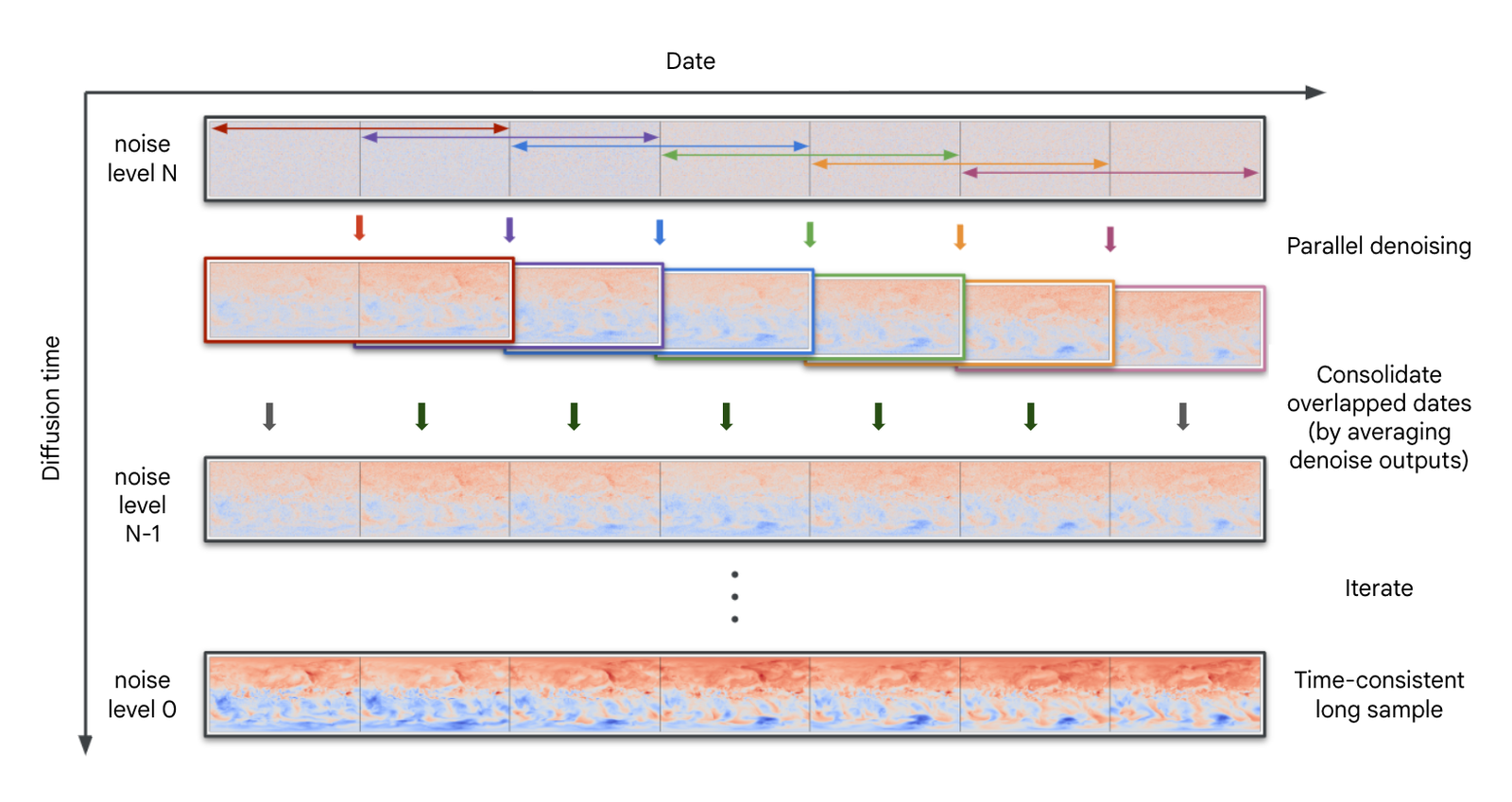
S2.2.5 Hyperparameters
Table S2 shows the set of hyperparameters used for the denoiser architecture, as well as those applied during the training and sampling phases of the diffusion model. We also include the optimization algorithm, learning rate scheduler and weighting for minimizing (S18).
| Denoiser architecture (output shape: equivalent to 3-day, bi-hourly samples) | |
|---|---|
| Downsampling ratios (spatial) | [3, 2, 2, 2] |
| Number of residual blocks per resolution | 4 |
| Hidden channels | [128, 256, 384, 512] |
| Axial attention layers in resolution | [False, False, True, True] |
| Training | |
| Device | TPUv5p, |
| Duration | 300K steps |
| Batch size | 128 (with data parallelism) |
| Learning rate | cosine annealed (peak=, end=), 1K linear warm-up steps |
| Gradient clipping | max norm = 0.6 |
| Noise sampling | LogUniform(min=, max=80) |
| Noise weighting () | |
| Condition dropout probability () | 0.15 |
| Inference (sample length: 33 days, bi-hourly) | |
| Device | TPUv5e, |
| Noise schedule | , |
| SDE solver type | 1st order exponential |
| Solver steps | |
| CFG strength () | 1.0 |
| Overlap | 1 day (12 time slices) |
S2.2.6 Training, evaluation, and test data
The super-resolution stage is trained independently of the debiasing stage, using perfectly time-aligned ERA5 data samples at the input (1.5-degree, daily) and output (0.25-degree, bi-hourly) resolutions.
Training is conducted on continuous 3-day periods randomly selected in the training range. Spatially, the model super-resolves a rectangular patch of fixed size, spanning 60∘ in longitude and 30∘ in latitude. Consistent with the debiasing step, data from 1960–2000 is used for training, 2001–2010 for evaluation, and 2011–2020 for testing.
S2.2.7 Computational cost
Training the diffusion model takes approximately 3 days on TPUv5p hosts with a total of 32 cores. Sampling is performed in parallel using 16 TPUv5e cores, where each core denoises a single 3-day period, collectively producing a 33-day temporally consistent long sample999With our parallel strategy, 33 days = number of cores [16] (model days [3] - overlap [1]) + overlap [1]; increasing the number of cores effectively increases the total length of days. Alternatively, one may sample 3-day periods sequentially, in which case the sample length does not vary with the number of cores and instead scales with inference time.. Each sample requires around 20 minutes to complete, including JAX compile time (generating additional realizations is significantly more time-efficient). The time length of the generated samples scales linearly with the number of TPU cores utilized, with clock time remaining roughly constant (albeit communication overhead amongst a large pool of devices may increase in a non-negligible way).
S2.3 Baselines
S2.3.1 Bias correction and spatial disaggregation (BCSD)
The Bias Correction and Spatial Disaggregation (BCSD) method is a standard algorithm for downscaling climate data [96]. In our setup, the method may be decomposed into three main stages: bias correction (BC), spatial disaggregation (SD) and temporal disaggregation (TD).
Bias correction based on Gaussian quantile mapping (QM). The goal of this step is to map the quantile of to that of the downsampled observation data :
| (S37) |
where the climatological mean and standard deviation are calculated over the training period (1960-2000). It is important to note that the quantiles for each LENS2member are computed relative to their own climatology. Unlike GenBCSR, which normalizes using the aggregated climatology of the limited set of training members, this method may favor BCSD due to its incorporation of a broader range of “training" data. The competitive performance of GenBCSR, despite this difference, highlights its robustness.
Spatial disaggregation. In the second stage, cubic interpolation is applied to the quantile, followed by adding the climatological mean of the full-resolution observations:
| (S38) |
This step yields outputs with the desired spatial resolution, while the temporal resolution remains at daily means.
Temporal disaggregation. The final stage involves randomly selecting a historical sample sequence from the high-resolution dataset covering the period represented by the spatially disaggregated data, in this case a day, and corresponding to the same time of the year, in this case the same day-of-year. The spatially disaggregated data is then substituted by this sequence after adjusting it to match the daily mean of the spatially disaggregated sample:
| (S39) |
This step ensures that the outputs achieve the target temporal resolution.
S2.3.2 Quantile mapping
The quantile mapping component of BCSD can be adapted as a near drop-in replacement for the debiasing step of GenBCSR. The only required modification is adding back the mean of the downsampled data:
| (S40) |
The resulting output retains the low spatial resolution and can serve as the input for our diffusion-based upsampling model. This is the “QM” baseline referred to in Table 1.
Appendix S3 Data
S3.1 Input Datasets
We are using the Community Earth System Model Large Ensemble (LENS2) dataset[47] for our low-resolution climate dataset. LENS2 was produced using the Community Earth System Model Version 2 (CESM2), a climate model that has interactive atmospheric, land, ocean, and sea-ice models [97]. LENS2 is configured to estimate historical climate and the future climate scenario, SSP3-7.0, following the CMIP6 protocol [98]. LENS2 skillfully represents the response of historical climate to external forcings [99]. LENS2 output is available from 1850-2100, with a horizontal grid spacing of 1∘, and 100 simulation realizations.
The ERA5 reanalysis dataset [31] is our high-resolution weather dataset. ERA5 uses a modern forecast model and data assimilation system with all available weather observations to produce an estimate of the atmospheric state. This estimate includes conditions ranging from the surface to the stratosphere. ERA5 data is available from 1940 to near present at a horizontal grid spacing of 0.25∘. ERA5 estimated extremes of temperature and precipitation agree well with observations in areas where topography changes slowly [100].
S3.2 Modeled variables
We explicitly model four variables in our downscaling pipeline: near-surface temperature, wind speed magnitude, specific humidity, and sea level pressure. The official names for these variables, as documented in the datasets, are listed in Table S3.
| Quantity | Unit | ERA5 variable | LENS2variable |
|---|---|---|---|
| Near-surface temperature | K | 2m_temperature | TREFHT |
| Near-surface wind speed magnitude | m/s | WSPDSRFAV | |
| Near-surface specific humidity | kg/kg | specific_humidity (level=1000 hPa) | QREFHT |
| Sea level pressure | Pa | mean_sea_level_pressure | PSL |
S3.3 Regridding
The ERA5 dataset is natively 0.25∘ and LENS2 is 1∘. Here we use linear interpolation to regrid the data to 1.5∘ using the underlying spherical geometry of the data, instead of performing interpolation in the lat-lon coordinates. We compute daily averages for both datasets.
Appendix S4 Evaluation
S4.1 Derived variables
Here we describe how the derived variables are calculated. In addition to the explicitly modeled variables, we utilize surface elevation, a static quantity, to convert sea level pressure to pressure at surface height.
Relative humidity. To calculate the relative humidity, we first compute the pressure at surface height using the barotropic formula
| (S41) |
where denotes the sea level pressure (Pa), is the surface temperature (K), is the standard lapse rate for temperature (0.0065 K/m), is the molar mass of air (0.02896 kg/mol), and are the gravitational acceleration (9.8 m/) and universal gas constant (8.31447 J/mol/K) respectively.
Next we compute the saturation vapor pressure using the August-Roche-Magnus formula
| (S42) |
and the actual vapor pressure
| (S43) |
where denotes specific humidity in kg/kg.
Finally, the relative humidity is expressed as the ratio of actual vapor pressure to the saturation vapor pressure:
| (S44) |
which will give RH as a percentage.
Heat index. The heat index [59] is a quantity defined by the National Oceanic and Atmospheric Administration (NOAA) which represents “what the temperature feels like to the human body when relative humidity is combined with the air temperature”. It is based on the regression equation:
| (S45) | ||||
where is temperature in degree Fahrenheit °F[101]. It is subject to additional adjustments [102]
| (S46) |
Furthermore, if the above yields a heat index below (300K), a simpler formula is used instead
| (S47) |
We compute the heat index by converting the input temperature to degree Fahrenheit first, and the resulting output heat index back to Kelvin.
Based on the heat index, NOAA also provides 4 advisory levels: caution, extreme caution, danger and extreme danger triggered by the heat index value exceeding , , and (300K, 305K, 312.6K, 325K) respectively.
S4.2 Metrics
S4.2.1 Pointwise distribution errors
The following metrics measure the distribution difference between a collection of predicted samples and a collection of reference samples , where .
Mean absolute bias (MAB). This metric measures the mean absolute difference between the means
| (S48) |
where and denotes the index over samples and dimensions respectively. and are the number of predicted and reference samples whose distributions are compared.
Wasserstein distance (WD).
To compute this metric, we compute the Wasserstein-1 metric for each pixel in the image, which is the norm between the predicted and reference distribution, and then we average it over the pixels in the image.
Algorithmically, this metric involves constructing empirical cumulative distribution functions CDF and for the predicted and reference samples respectively. The Wasserstein distance is then computed as an empirical integral:
| (S49) |
where represent the quadrature points over which the integrand is evaluated for dimension . These points are chosen to cover the union of the support for both predicted and reference distributions.
Percentile mean absolute error (MAE). This metric measures the mean absolute difference between the th percentiles of the predicted and reference samples:
| (S50) |
S4.2.2 Correlations
Spatial correlation. Given scalar samples at a specific target location and samples at its nearby location ( and denote the neighbor index), the correlation coefficient is computed as
| (S51) |
where denotes the sample mean.
Computing the correlation coefficient across all nearby locations within a selected range yields the correlation matrix . The spatial correlation error is then quantified using the Frobenius norm of the difference between the predicted and reference correlation matrices:
| (S52) |
Temporal spectra. The temporal correlation can be analyzed through the power spectral density:
| (S53) |
where represents the length of the time series in physical units, is the th frequency component and is the Discrete Fourier Transform of . To characterize the temporal correlation for an ensemble, we take the average across its members. The error between the predicted and reference spectra is quantified by the mean log ratio difference:
| (S54) |
where denotes the number of frequency components considered in the Fourier Transform.
S4.2.3 Compound events
Heat streaks. The heat streak probability in Figure 4 is defined as the probability of any day being part of a continuous -day span, such that the daily maximum temperature is above the climatological daily maximum plus a threshold. Given a time series of daily maximum temperatures , the probability can be calculated by carrying out the following steps:
-
1.
Identify all indices such that . Include the days in the count of days.
-
2.
Count the unique days that appear in any such streak across the time series.
-
3.
Let denote the set of unique days that are part of a -day streak with daily maximum temperatures greater than threshold. Then
(S55)
The error is then quantified as the mean squared error between the predicted and reference streak probability:
| (S56) |
where the mean is taken across all locations in the area of study.
Tropical cyclones. Cyclones are detected using the TempestExtremes [103] framework with the following criteria:
-
•
Time slices are analyzed at 6-hour intervals (i.e. downsampling factor of 3 with respect to our output time resolution).
-
•
Local minima in sea level pressure (SLP) are identified, requiring an SLP increase of at least 240 Pa within a 4.0 great circle distance (GCD). Smaller minima within a 2.0 GCD are merged.
-
•
Wind speed must exceed 10 m/s for a minimum of 8 snapshots. The surface elevation of the minima must remain below 100 m for the same duration.
-
•
The minima must persist for at least 54 hours, with a maximum gap of 24 hours in the middle.
-
•
The maximum allowable distance between points along the same path is 8.0 GCD.
It is important to note that detecting tropical cyclones usually requires further filtering based on upper-level geopotential gap or temperature thresholds to identify warm-core structures. Such qualifications are excluded from the definition above, as our emphasis is placed on downscaling near-surface variables. Nonetheless, the criteria remain consistent for both predicted and reference samples, and provide a representative assessment of the associated risks.
Cyclone density (such as that in Figure 4 (K)) is derived from tracks identified using the above criteria. Each pixel along a cyclone track is replaced with a spherical Gaussian density function, centered at the pixel with a standard deviation of 1 GCD. The resulting densities are then averaged across all ensemble members to produce the final density map.
Appendix S5 Ablation studies
S5.1 Sensitivity to training range
S5.1.1 Debiasing
Table S4 shows the pointwise aggregated distributional metrics for a few different debiasing models: one trained over the full range (1961-2000) and ones trained with subsets of various lengths (10 to 30 years). We observe mixed sensitivity, with errors being larger for temperature and humidity using less data, but smaller for sea-level pressure. This suggests that data quality is critically important for the performance of the debiasing step and the overall downscaling pipeline.
In addition, Figures S3 and S4 show the seasonal bias (as explained in S7.1.2) for the models trained with different data for the 2-meter temperature and mean sea level pressure, respectively. For the former, we can observe that although their training sets are different, the biases have a similar geographical distribution, although with different intensities. E.g., on average, all the debiasing models forecast a colder winter in the Northern Hemisphere and a warmer fall in North America and Europe. In contrast, from Figure S4, we observe that the geographical distribution of the trend bias is fairly consistent with models trained with data from the decade of the 1960s. However, for the model trained without data from that decade, we can observe a change in the pattern of the bias. This further suggests that the quality of the data is key for the performance of the debiasing step.
Finally, we study the impact of the training data on the projection of the seasonal mean well beyond the training range. Figure S5 shows the zonal seasonal mean of the 2-meter temperature within the region between 55°N and 55°S (this is chosen to avoid the ice caps, as mentioned in S7.1.2). The different models agree in the range 1960 to 2000 and are mostly driven by the climate model (LENS2) afterwards. However, they begin to diverge as we approach the end of the century. This suggests that our debiasing technique generally follows the trend imposed by the unbiased data, and some global statistics remain fairly stable on the training data. Nevertheless, there is an increasing bias, which becomes more noticeable for larger leading times.
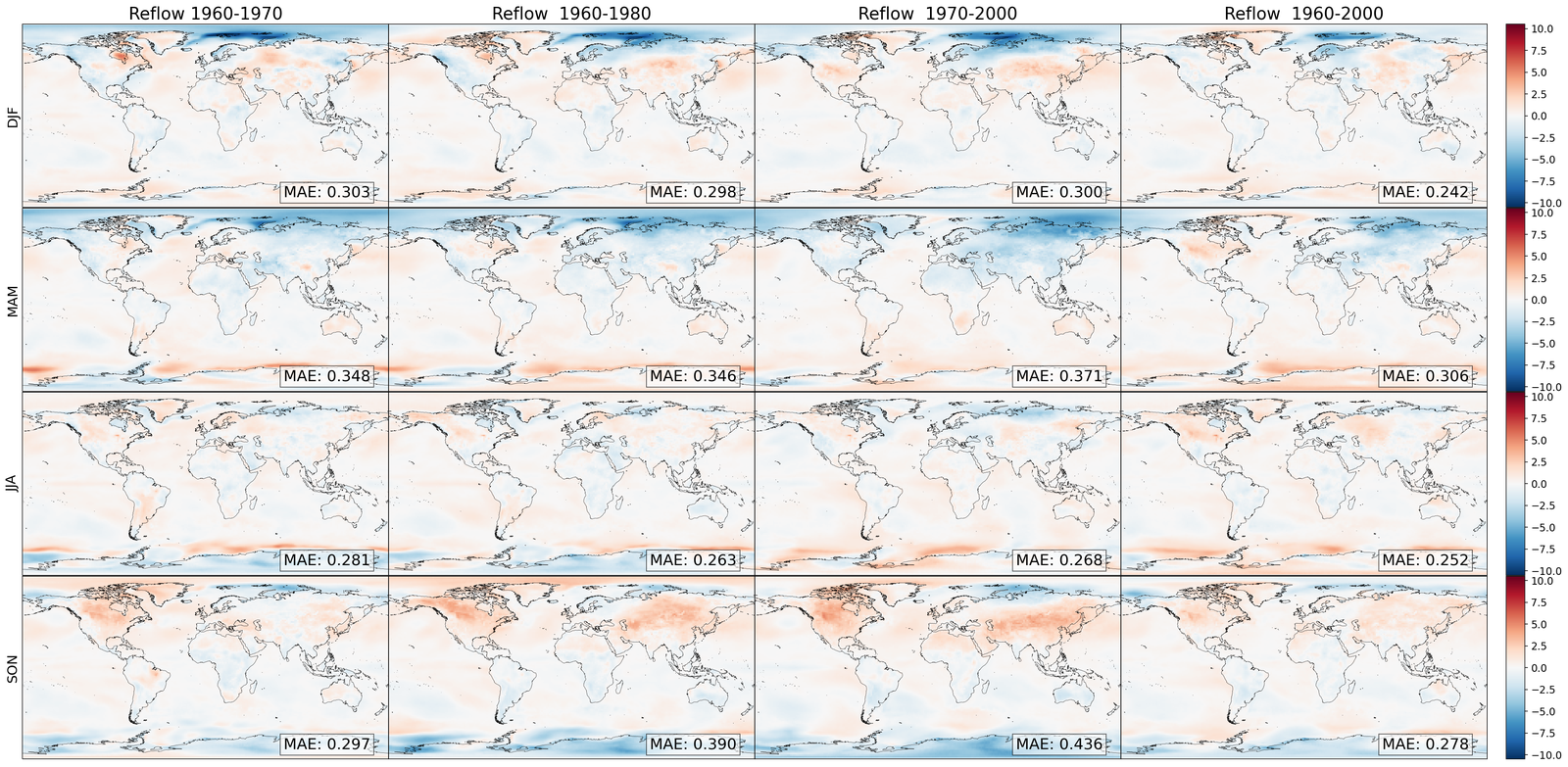
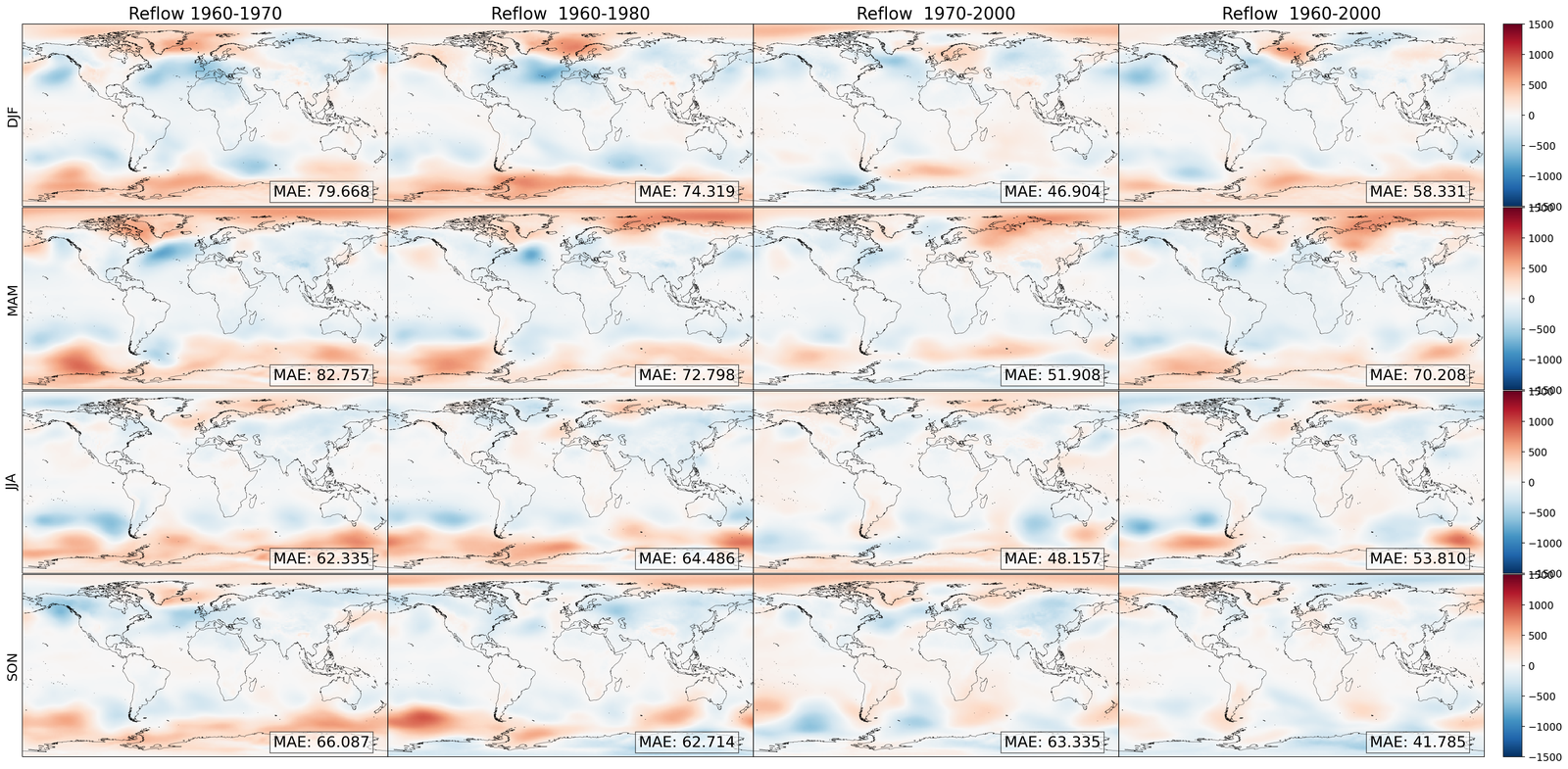
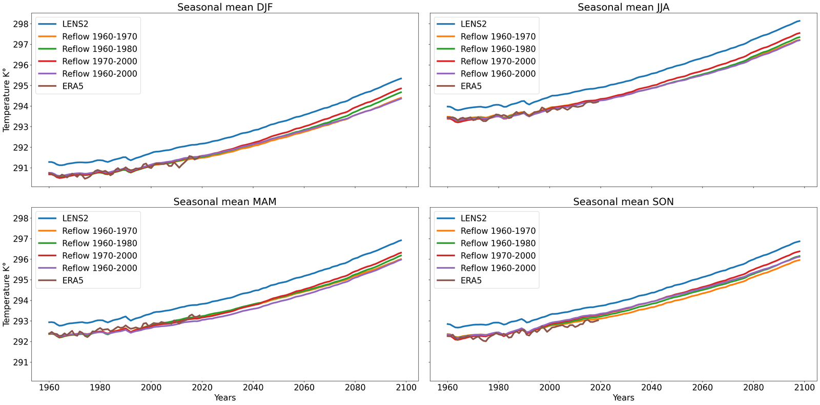
| Mean Absolute Bias | Wasserstein Distance | Mean Absolute Error, 99% | ||||||||||
|---|---|---|---|---|---|---|---|---|---|---|---|---|
| Number of training years | 40 | 30 | 20 | 10 | 40 | 30 | 20 | 10 | 40 | 30 | 20 | 10 |
| Temperature (K) | 0.74 | 0.83 | 0.74 | 0.77 | 0.79 | 0.87 | 0.79 | 0.81 | 0.88 | 0.95 | 1.02 | 1.11 |
| Wind speed (m/s) | 0.19 | 0.18 | 0.18 | 0.17 | 0.28 | 0.27 | 0.27 | 0.26 | 0.64 | 0.64 | 0.67 | 0.63 |
| Specific humidity (g/kg) | 0.49 | 0.56 | 0.53 | 0.52 | 0.55 | 0.61 | 0.60 | 0.59 | 0.56 | 0.61 | 0.62 | 0.74 |
| Sea-level pressure (Pa) | 68.28 | 63.26 | 58.23 | 53.81 | 67.46 | 63.79 | 60.60 | 57.37 | 97.31 | 87.31 | 85.21 | 80.59 |
| Relative humidity (%) | 2.89 | 2.48 | 3.64 | 3.22 | 3.12 | 2.75 | 3.81 | 3.42 | 3.05 | 2.83 | 3.75 | 3.66 |
| Heat index (K) | 0.58 | 0.60 | 0.67 | 0.67 | 0.64 | 0.67 | 0.73 | 0.64 | 1.35 | 1.31 | 1.26 | 1.14 |
S5.1.2 Upsampling
Table S5 shows a similar comparison, but for upsampling model trained with different date ranges. The metrics exhibit much less sensitivity to the training range, especially for the mean bias and Wasserstein distance. Tail statistics, on the other hand, may still benefit from more training data.
Based on these observations, the debias-then-upsample factorization can be interpreted in an alternative way: the debiasing step inherently incorporates non-stationary corrections that are sensitive to temporal variability and the physical states represented in the base simulations being downscaled. This step reflects adjustments that respond to changing climatological conditions and specificities within the training period. On the other hand, the upsampling step appears to be more static, characterized by its reliance on spatial interpolation and transformation methods that are less dependent on temporal dynamics and, therefore, more statistically generalizable across different time frames.
| Mean Absolute Bias | Wasserstein Distance | Mean Absolute Error, 99% | ||||||||||
|---|---|---|---|---|---|---|---|---|---|---|---|---|
| Number of training years | 40 | 30 | 20 | 10 | 40 | 30 | 20 | 10 | 40 | 30 | 20 | 10 |
| Temperature (K) | 0.74 | 0.76 | 0.76 | 0.76 | 0.79 | 0.82 | 0.82 | 0.81 | 0.88 | 0.89 | 0.86 | 0.95 |
| Wind speed (m/s) | 0.19 | 0.21 | 0.20 | 0.19 | 0.28 | 0.32 | 0.31 | 0.28 | 0.64 | 0.71 | 0.73 | 0.68 |
| Specific humidity (g/kg) | 0.49 | 0.51 | 0.50 | 0.49 | 0.55 | 0.59 | 0.58 | 0.56 | 0.56 | 0.51 | 0.51 | 0.61 |
| Sea-level pressure (Pa) | 68.28 | 68.18 | 67.36 | 67.09 | 67.46 | 67.48 | 67.11 | 65.49 | 97.31 | 106.53 | 102.72 | 104.53 |
| Relative humidity (%) | 2.89 | 3.02 | 3.00 | 2.93 | 3.12 | 3.35 | 3.27 | 3.19 | 3.05 | 4.28 | 4.06 | 3.89 |
| Heat index (K) | 0.58 | 0.61 | 0.59 | 0.58 | 0.64 | 0.70 | 0.69 | 0.67 | 1.35 | 1.62 | 1.57 | 1.38 |
S5.1.3 Training with different decades
Table S6 shows the aggregated pointwise distributional metrics from GenBCSR models trained on data from different decades between 1960 and 2000. Interestingly, there is no consistent pattern for which decade minimizes error across all variables. Temperature and humidity errors decrease when training data is closer to the test period (2010s), while wind speed and pressure show better performance when trained on data from the 1980s and pre-1980s, respectively. However, the tail statistics (in terms of the 99th percentile MAE) generally improves as more data is included. This suggests that using the full range of training data, rather than focusing solely on recent periods, enhances coverage of extreme events.
| Mean Absolute Bias | Wasserstein Distance | Mean Absolute Error, 99% | |||||||||||||
|---|---|---|---|---|---|---|---|---|---|---|---|---|---|---|---|
| Training period | 60s | 70s | 80s | 90s | full | 60s | 70s | 80s | 90s | full | 60s | 70s | 80s | 90s | full |
| Temperature (K) | 0.83 | 0.83 | 0.77 | 0.71 | 0.74 | 0.83 | 0.82 | 0.81 | 0.69 | 0.79 | 1.17 | 1.15 | 1.03 | 0.88 | 0.88 |
| Wind speed (m/s) | 0.20 | 0.20 | 0.16 | 0.19 | 0.19 | 0.26 | 0.26 | 0.23 | 0.24 | 0.28 | 0.68 | 0.71 | 0.68 | 0.66 | 0.64 |
| Specific humidity (g/kg) | 0.59 | 0.58 | 0.55 | 0.53 | 0.49 | 0.62 | 0.62 | 0.59 | 0.56 | 0.55 | 0.72 | 0.73 | 0.75 | 0.76 | 0.56 |
| Sea-level pressure (Pa) | 44.40 | 44.26 | 36.24 | 72.19 | 68.28 | 52.90 | 52.62 | 47.70 | 66.38 | 67.46 | 79.03 | 78.47 | 68.41 | 104.42 | 97.31 |
| Relative humidity (%) | 4.06 | 4.05 | 3.22 | 2.78 | 2.89 | 4.30 | 4.34 | 3.54 | 3.05 | 3.12 | 4.56 | 5.25 | 5.22 | 4.82 | 3.05 |
| Heat index (K) | 0.83 | 0.83 | 0.59 | 0.67 | 0.58 | 0.89 | 0.89 | 0.67 | 0.72 | 0.64 | 1.53 | 1.53 | 1.11 | 1.21 | 1.35 |
Case study: tropical cyclone risks.
We further examine the effect of the training data range on cyclone statistics in the CONUS region. Figure S6 shows the cyclone counts and density contours in the Gulf of Mexico, resulted from training the GenBCSR pipeline using data from different decades spanning from the 1960s to the 1990s, with inference performed in the 2010s. The statistics exhibit considerable sensitivity to the training period, with models trained on later decades producing cyclone counts closer to ERA5 observations. The associated risk, quantified as the average cyclone density over land pixels in the area, also increases with training data from later decades. The shift from the 1970s to the 1980s is particularly notable, resulting in more than a doubling of the risk Notably, the transition from the 1970s to the 1980s results in more than a doubling of the risk. This shift can be partially attributed to the introduction of satellite data in ERA5 during the 1980s. It may also reflect significant changes in climate conditions during this period.
These findings highlight the capability of GenBCSR to reproduce historical trends and provide valuable insights into the risks associated with historical and ongoing climate change. By leveraging a wide range of training data, GenBCSR provides a robust framework for understanding the evolving climate system and its associated impacts.
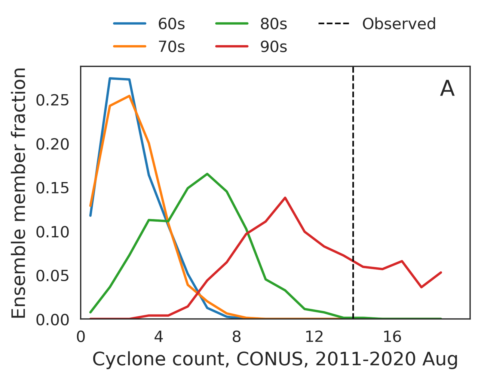
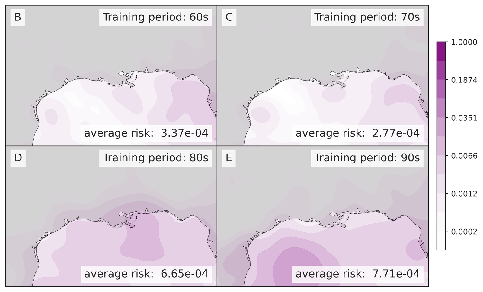
S5.2 Upsampling unbiased inputs
Table S7 compares the distributional metrics between the unpaired downscaling setup, which uses debiased LENS2as input, and the paired downscaling setup, which utilizes the ground truth coarse-scale ERA5 as input. The paired setup yields significantly lower errors than the unpaired setup, demonstrating the strong performance of our upsampling model when provided with accurate and unbiased inputs. It is important to reiterate that such ideal input data cannot be expected in practical scenarios. Therefore, the ability to correct biases in the input data is essential for the overall effectiveness of the downscaling pipeline.
| Mean Absolute Bias | Wasserstein Distance | Mean Absolute Error, 99% | ||||
|---|---|---|---|---|---|---|
| Unpaired | Paired | Unpaired | Paired | Unpaired | Paired | |
| Temperature (K) | 0.74 | 0.07 | 0.79 | 0.13 | 0.88 | 0.28 |
| Wind speed (m/s) | 0.19 | 0.066 | 0.28 | 0.08 | 0.64 | 0.23 |
| Specific humidity (g/kg) | 0.49 | 0.041 | 0.55 | 0.069 | 0.56 | 0.088 |
| Sea-level pressure (Pa) | 68.28 | 2.28 | 67.46 | 7.19 | 97.31 | 13.39 |
| Relative humidity (%) | 2.89 | 0.39 | 3.12 | 0.72 | 3.05 | 1.42 |
| Heat index (K) | 0.58 | 0.09 | 0.64 | 0.15 | 1.35 | 0.32 |
Appendix S6 Additional evaluation results
S6.1 CONUS
In this section, we include additional evaluation results in the Conterminous United States (CONUS) region, defined by latitude-longitude range with longitudes spanning from 126∘W to 66∘W and latitudes extending from 22.5∘N to 52.5∘N.
Distribution errors. Figure S7 shows the comparison of pointwise distribution errors (aggregated values corresponding to Table 1) for all variables between GenBCSR and BCSD. Table S8 details the MAE at additional high percentiles. Overall, the advantage of GenBCSR becomes increasingly evident at more extreme percentiles.
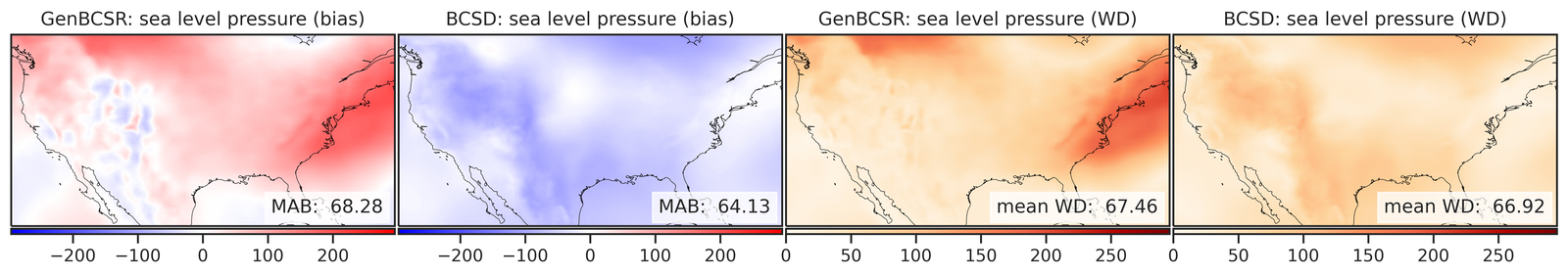
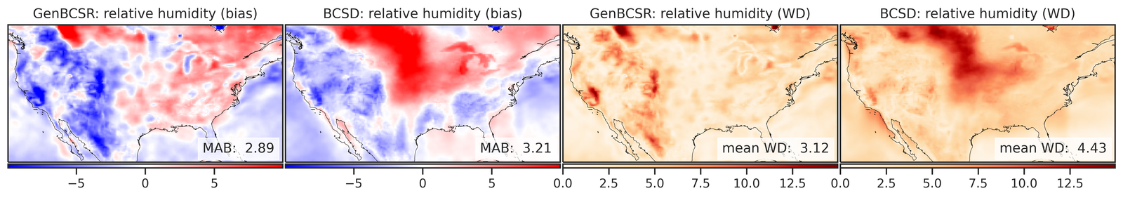
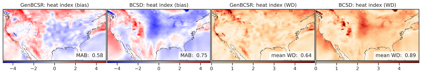
| GenBCSR | BCSD | |||||||||||
|---|---|---|---|---|---|---|---|---|---|---|---|---|
| Percentile | 75 | 80 | 85 | 90 | 95 | 99 | 75 | 80 | 85 | 90 | 95 | 99 |
| Temperature (K) | 0.78 | 0.79 | 0.82 | 0.84 | 0.86 | 0.88 | 0.77 | 0.79 | 0.82 | 0.86 | 0.93 | 1.07 |
| Wind speed (m/s) | 0.29 | 0.30 | 0.32 | 0.35 | 0.42 | 0.64 | 0.27 | 0.28 | 0.30 | 0.33 | 0.38 | 0.73 |
| Specific humidity (g/kg) | 0.55 | 0.53 | 0.52 | 0.51 | 0.51 | 0.56 | 0.55 | 0.55 | 0.56 | 0.59 | 0.64 | 0.81 |
| Sea-level pressure (Pa) | 70.58 | 74.20 | 79.89 | 85.89 | 91.25 | 97.31 | 64.71 | 68.26 | 73.69 | 82.39 | 96.90 | 133.29 |
| Relative humidity (%) | 3.52 | 3.40 | 3.21 | 2.95 | 2.71 | 3.05 | 4.33 | 4.11 | 4.03 | 4.48 | 6.42 | 14.00 |
| Heat index (K) | 0.59 | 0.64 | 0.71 | 0.81 | 0.98 | 1.35 | 0.76 | 0.84 | 0.93 | 1.05 | 1.24 | 1.77 |
Spatial correlation. Figures S8, S9, and S10 show the spatial correlation plots for more selected cities and variables in the CONUS region. The advantage of GenBCSR over BCSD is generally consistent across all comparisons.
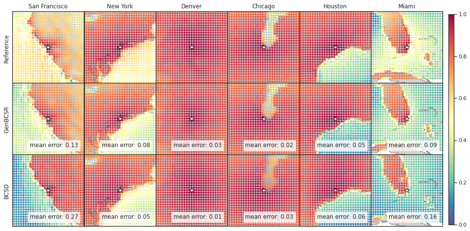
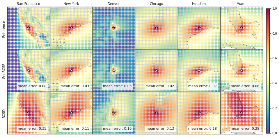
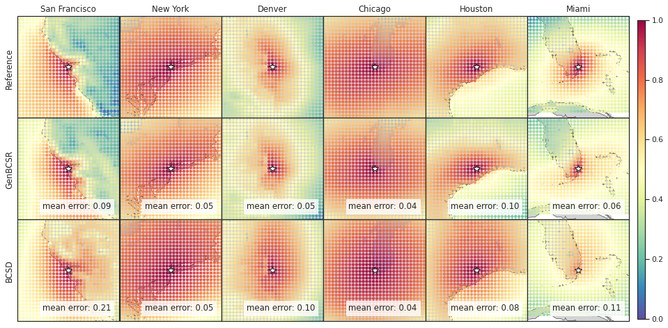
Temporal correlation. Figure S11 presents the power spectral densities and corresponding errors (definition in S4.2.2) for selected major cities in the CONUS region. Across all variables, GenBCSR demonstrates generally lower errors compared to BCSD, with particularly notable improvements in the low-frequency components of the wind speed and the high-frequency components of humidity.
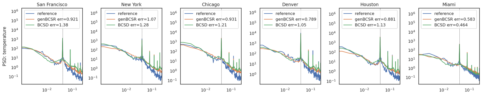
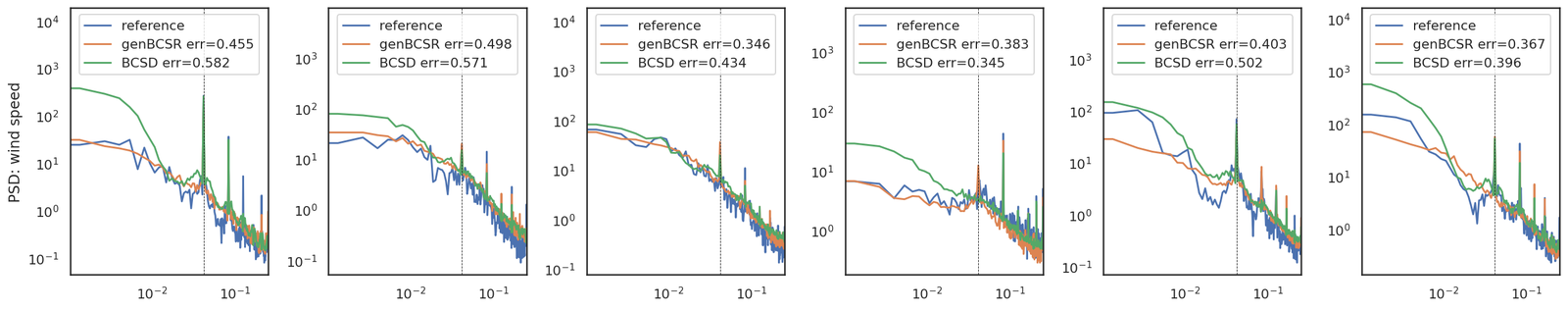
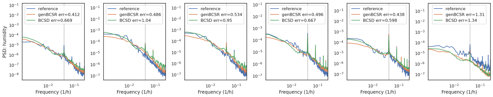
Heat advisory probability. Figure S12 shows the pointwise predictions and errors for the four different heat advisory levels (see S4.1). Across all four advisory levels, GenBCSR consistently exhibits lower error, highlighting its effectiveness in accurately predicting heat advisory conditions in the region.
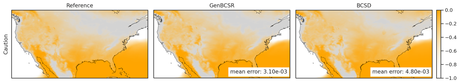
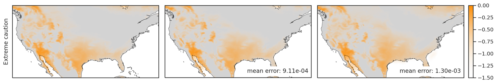
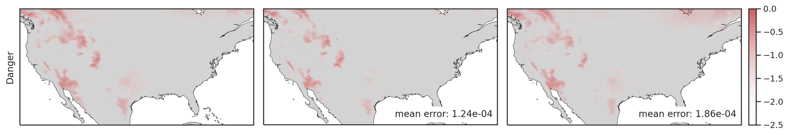
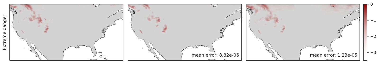
Heat streaks. Table S9 shows the heat streak probabilities for varying number of streak days and thresholds. We observe that the performance advantage of GenBCSR over BCSD extends to all configurations.
| 5°F > climatology | 10°F > climatology | |||
|---|---|---|---|---|
| Number of streak days | GenBCSR | BCSD | GenBCSR | BCSD |
| 2 | 0.0084 | 0.056 | 0.0014 | 0.012 |
| 3 | 0.0081 | 0.057 | 0.00090 | 0.0096 |
| 7 | 0.0041 | 0.041 | 0.00015 | 0.0027 |
S6.2 South Asia
In this section, we present additional evaluation results for the South Asia region, defined by the latitude-longitude range with longitudes spanning from 60∘E to 120∘E and latitudes extending from the equator (0∘N) to 30∘N. These results are based on the same global debiasing model used for CONUS, paired with an upsampling model specifically trained for the South Asia region.
Distribution errors. Figure S13 displays the pointwise distribution errors for all variables. The conclusions drawn from the CONUS region largely hold here: BCSD demonstrates lower errors than gen BCSR for the modeled variables, while GenBCSR outperforms or closely matches BCSD for the derived variables.
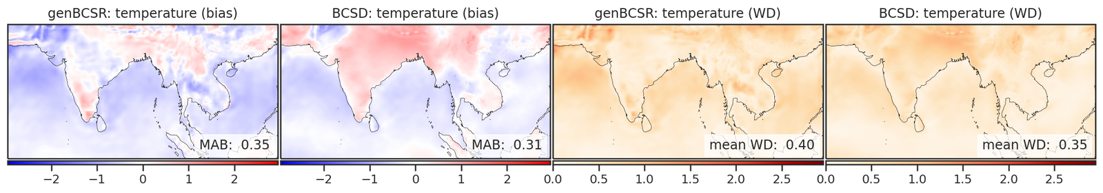
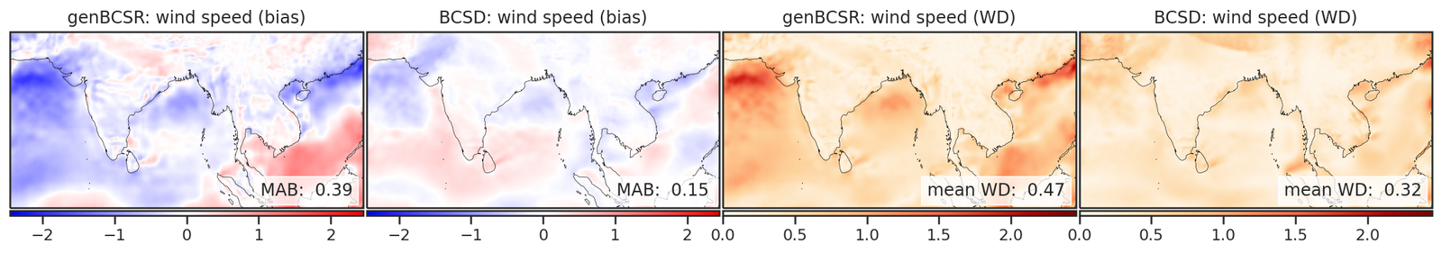
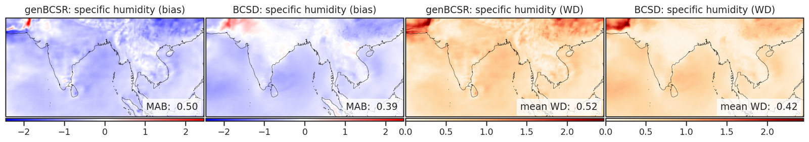
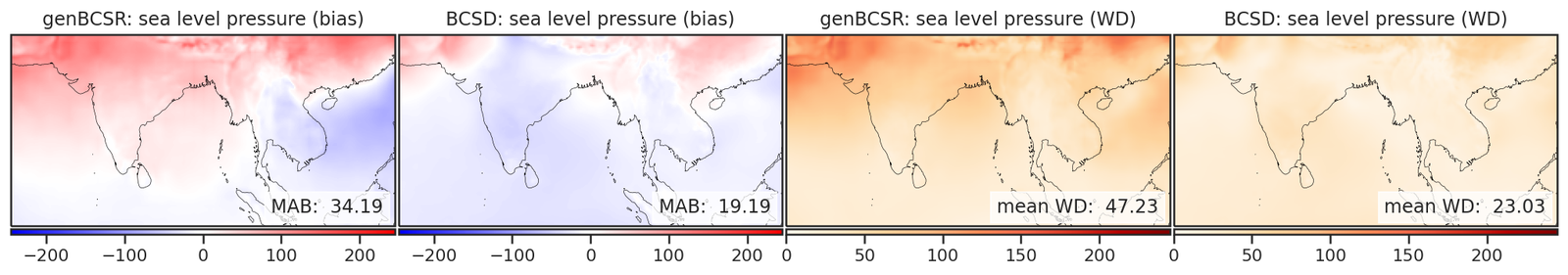
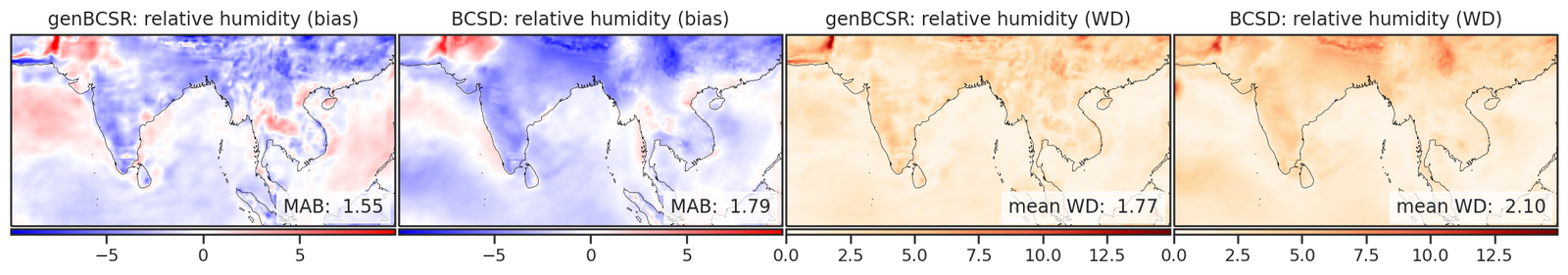
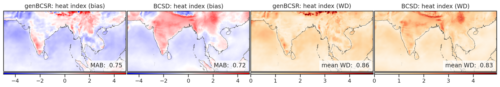
Spatial correlation. Figures S14, S15, and S16 presents the spatial correlation plots for selected cities in the region. The patterns produced by GenBCSR closely align with observed data at every test site, demonstrating its ability to accurately represent local geographic and meteorological structures.
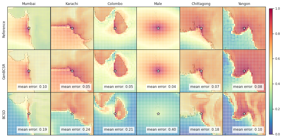
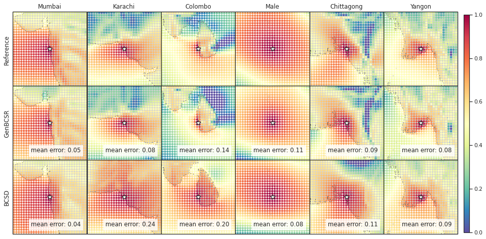
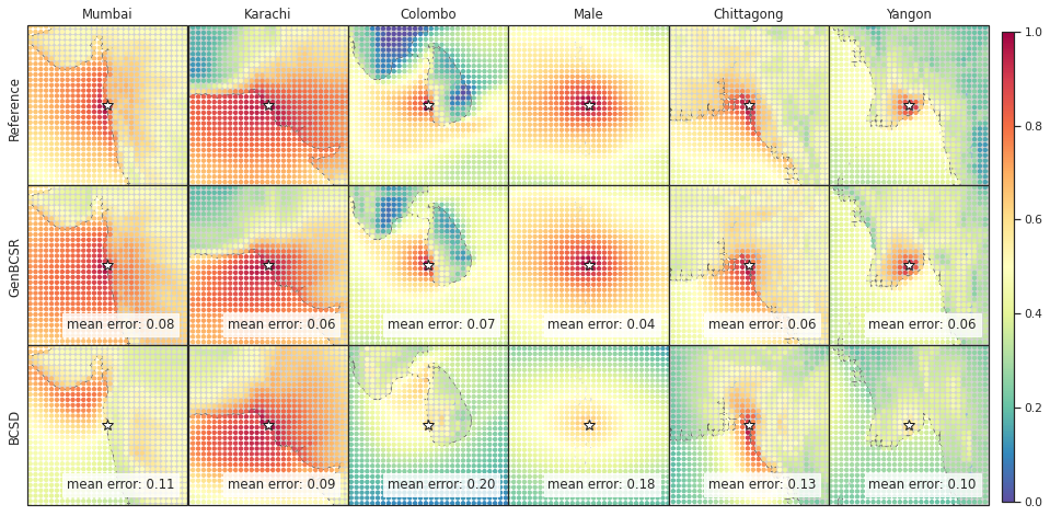
Combined with similar results shown for the CONUS region, this suggests that GenBCSR’s ability to capture realistic spatial correlation patterns is robust and transferable across diverse geographic domains.
Temporal correlation. Figure S17 presents the temporal power spectral density (PSD) plots for selected cities in the South Asia region. The results indicate that GenBCSR and BCSD perform comparably, with both methods capturing the overall temporal variability across different frequency ranges.
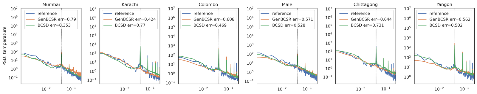
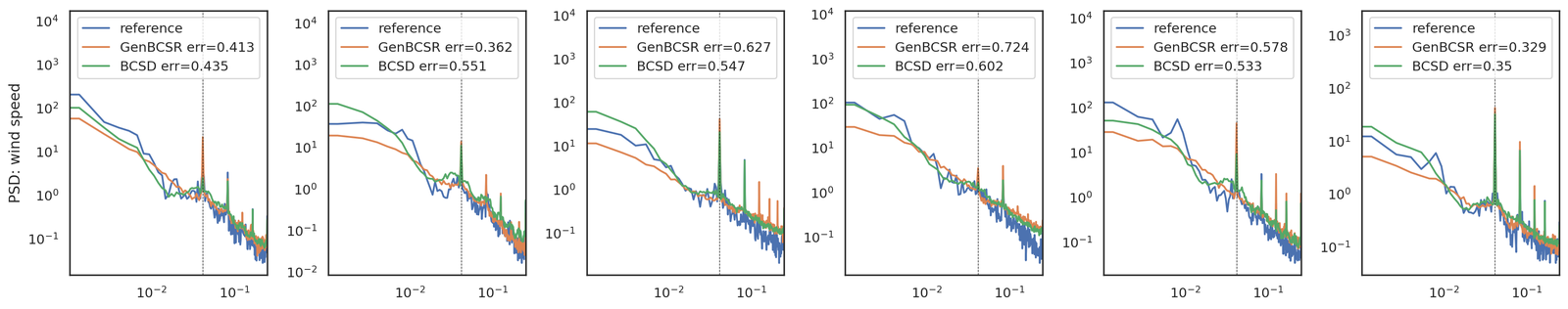
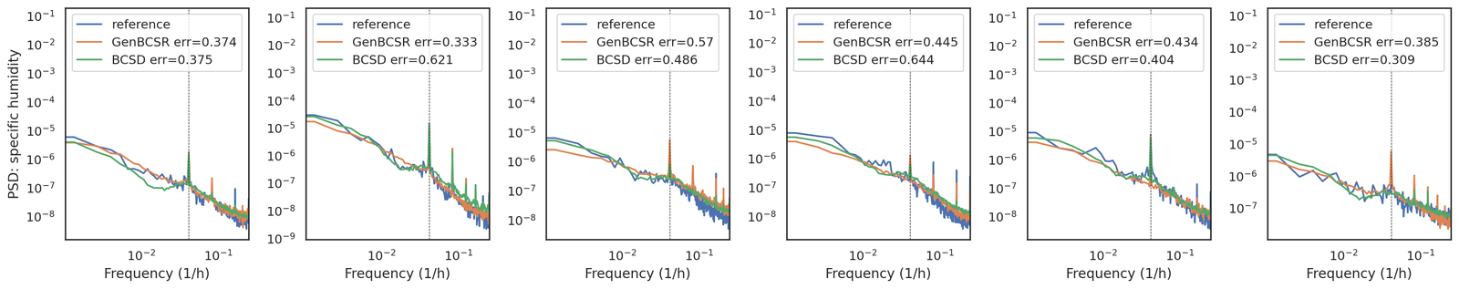
Heat advisory. Figure S18 shows the heat advisory probabilities in the area. GenBCSR has similar or better errors in all four advisory levels.
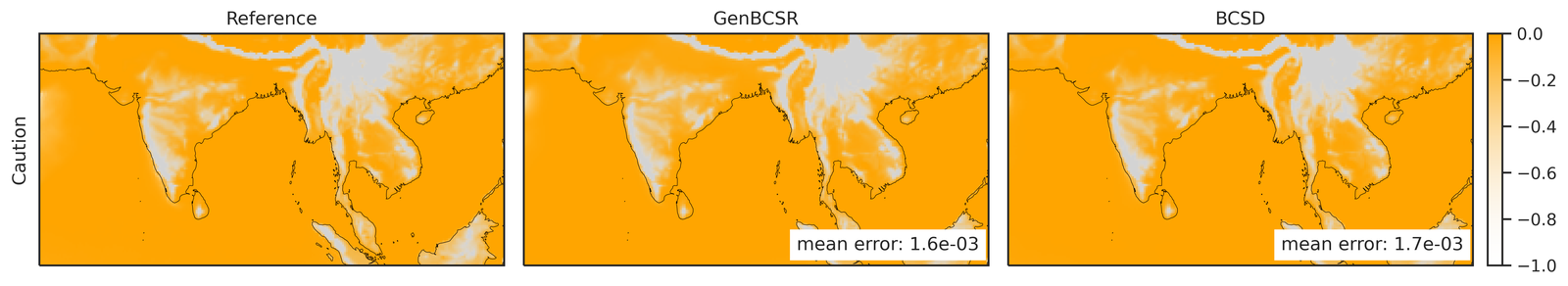
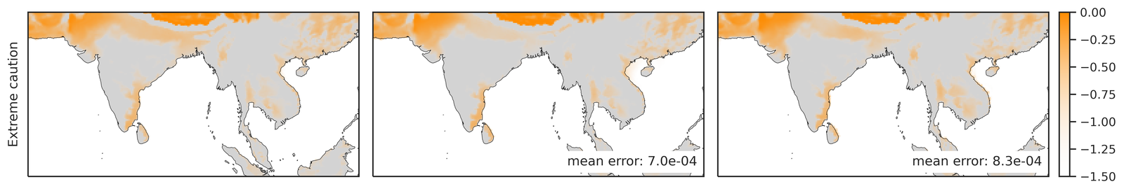
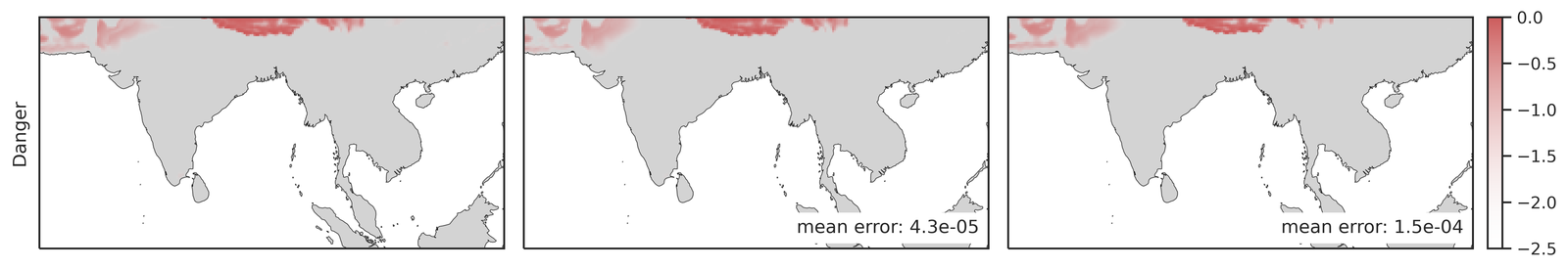
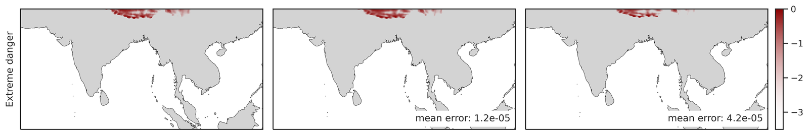
The performance advantage of GenBCSR in South Asia, while evident in certain aspects such as spatial correlation, is generally less pronounced compared to its performance in the CONUS region. This disparity may be attributed to the fact that model selection and hyperparameter tuning were primarily conducted with respect to the CONUS region, potentially leading to suboptimal configurations for South Asia’s unique climatic and geographic features. Nevertheless, the strong results in spatial correlation suggest that GenBCSR possesses transferable traits that adapt well to diverse regions, even without region-specific optimization. Future work could focus on tailoring model selection processes to regional characteristics, further enhancing performance in varied geographic contexts.
Appendix S7 Analyses
S7.1 Debiasing
In this section we provide further details on the effects of the different debiasing techniques considered in the main manuscript.
S7.1.1 Global trends
Here we further consider the global trends of the debiased quantities as a zonal weighted average between North and South. We compute the averages considering the spherical geometry of the data. The zonal mean is used to avoid the model (CESM in this case) uncertainty in the ice caps.
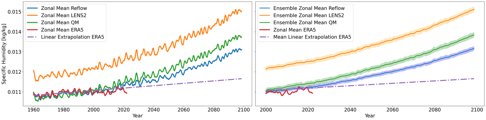
The ensemble zonal averages are computed as follows. For each ensemble member, the weighted average of the target quantity is computed daily. This yields a time series for each member, then a rolling time average is then computed using a rolling window of one year. This is equivalent to convolving the time series with a hat filter of width 365 days and a height of 1/365, creating a smoother time series for each member that reduces sub-seasonal effects. For each day of the time series (after cropping half a year at the beginning and end of the 140 years), the ensemble mean and standard deviation are computed. Figure 5 summarizes the evolution of zonal ensemble means for the 2-meter temperature, while Figure S19 summarizes the results for specific humidity.
Here we are seeking to capture the average out-of-distribution behavior of the debiasing step. Figure S19 showcases this behavior for the surface mean specific humidity, where we can observe that the debiased does correct the mean of LENS2 towards the mean of ERA5 during the training period, and it is then driven by LENS2 in the evaluation period and beyond. In addition, we can observe that the variability of the mean is kept roughly constant when the LENS2 data is debiased.
S7.1.2 Seasonal means
In addition we consider global ensemble means for different seasons when compared to QM for data in the testing dataset.
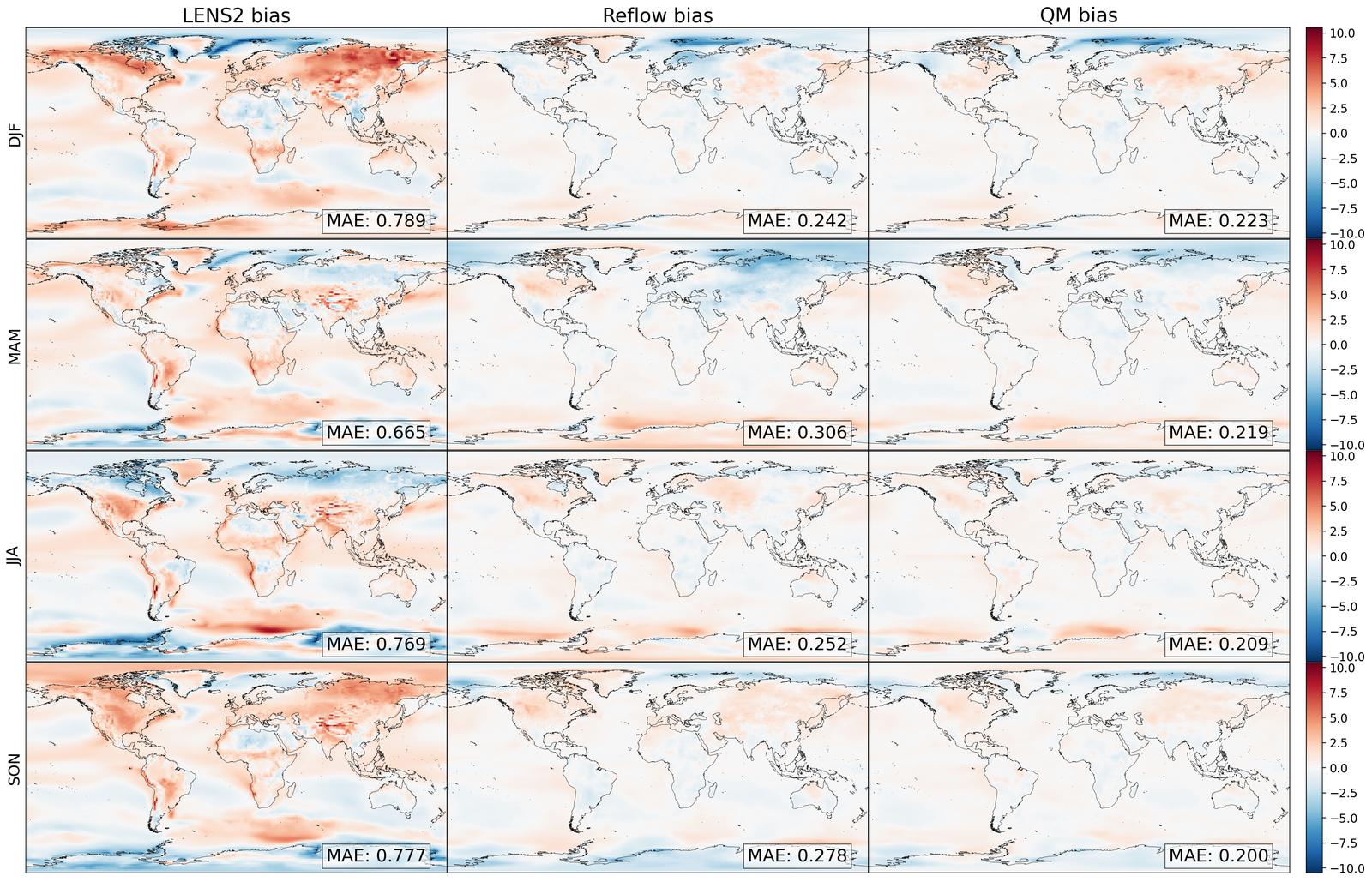
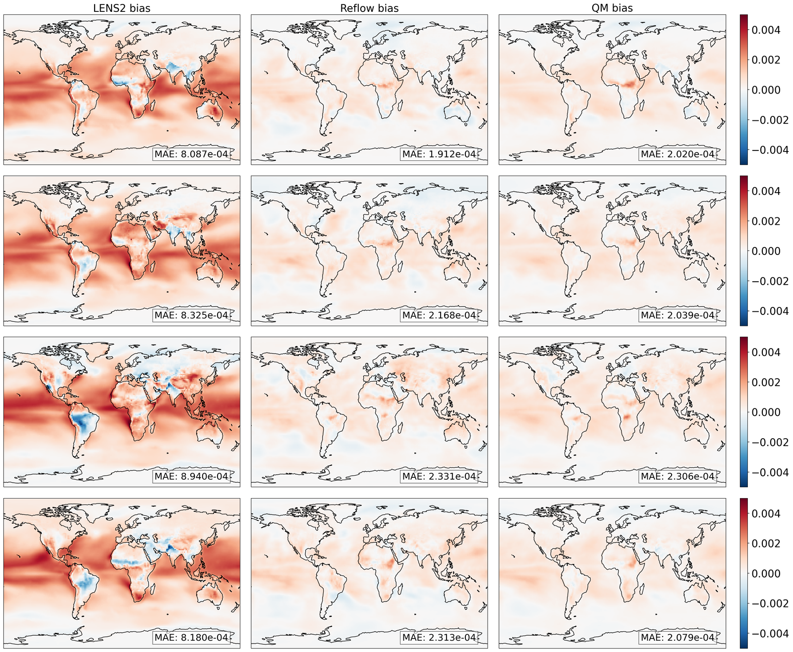
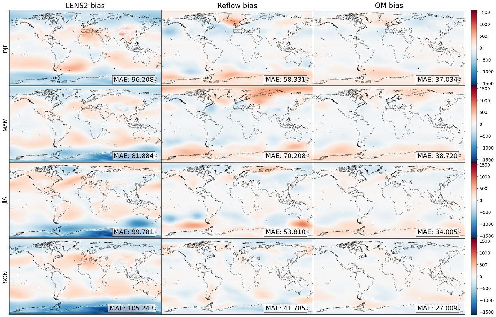
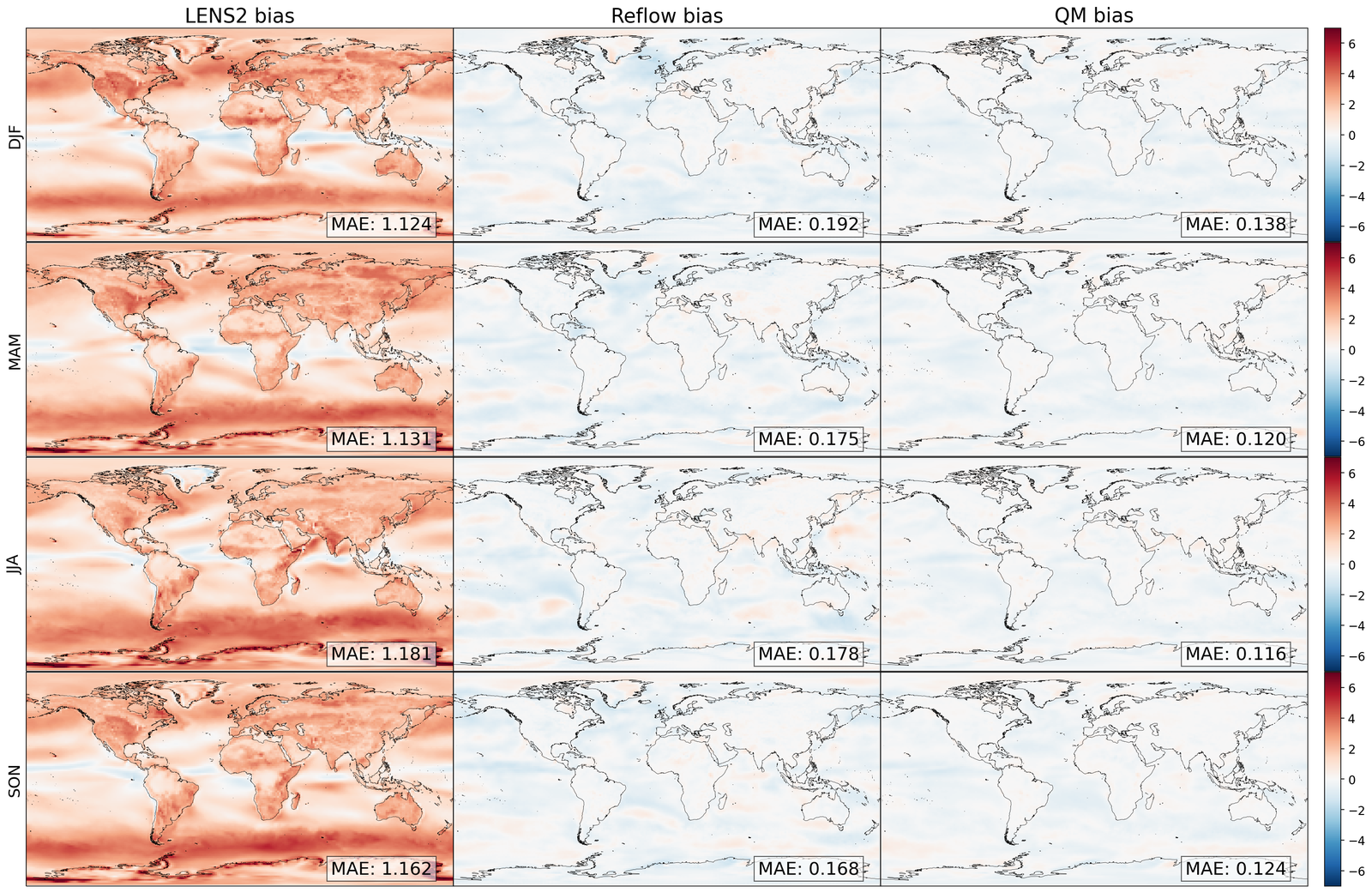
In Figure S20 we show the seasonal decadal means for the 2-meter temperature. We can observe that both quantile mapping and our reflow debiasing greatly correct the error in the LENS2ensemble. Following the trend in the Table 1 we observe that our method is competitive with QM particular far from the poles. In addition, we observe a similar pattern of geographical distribution of the bias across the different seasons.
We also show the seasonal decadal means for the surface specific humidity, mean sea level pressure, and 10-meter wind speed in Figures S21, S22, and S23, respectively. The same pattern can be seen, in which the bias seems to be concentrated close to the poles, and majority in the oceans.
We also consider the evolution of the seasonal zonal means in Figure S24. Figure S24 shows that as before the bias correction moves the zonal mean closer to the ground truth, and it is then driven by the climate model. We also compare the it to the seasonal trend predicted by QM, showing that they align relatively closely.
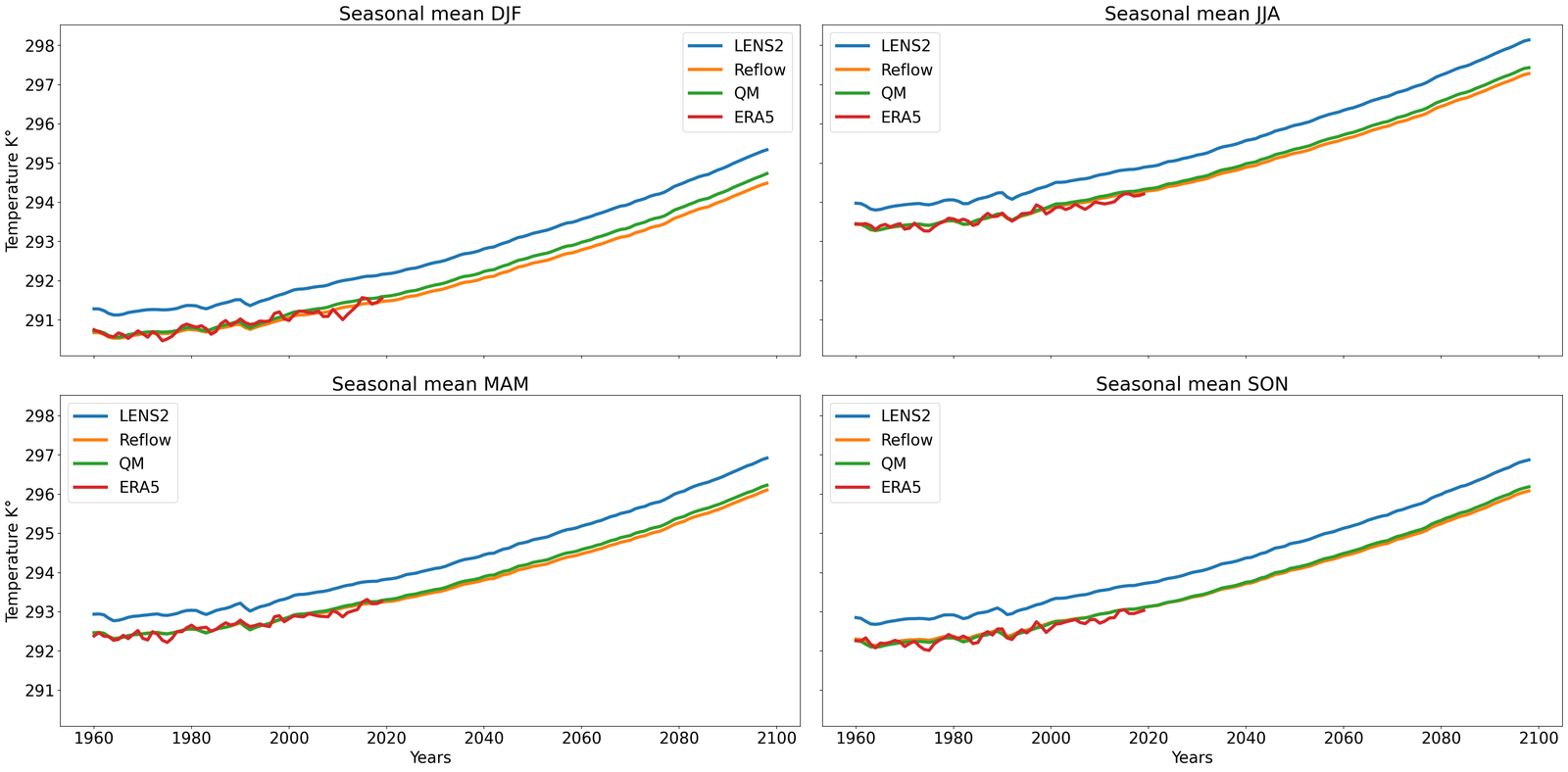
S7.1.3 Evolution of CONUS seasonal means
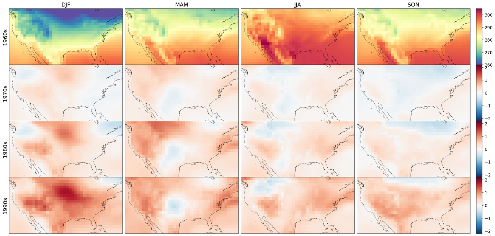
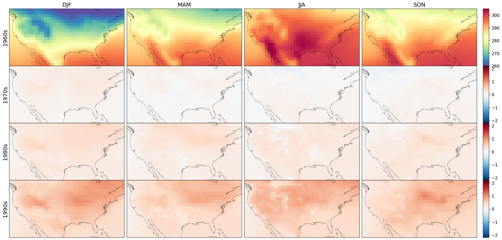
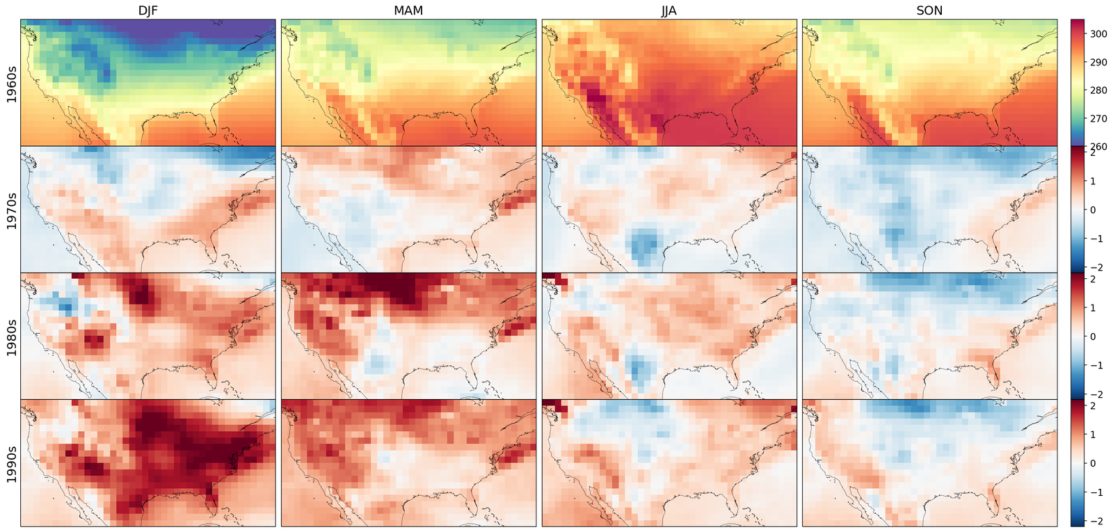
We study the evolution of ensemble decadal means forecasted by our method.
First we start comparing seasonal means of data during the training years of our model. Here we use the full ensemble consisting of the full 100 members to compute the means. As our model is only trained on only 4 ensembles this already constitutes a generalization task. Figure S25 shows the evolution of the ensemble decadal mean of the 2-meter temperature for the training decades, averaged over the 100 members of the ensemble. Figure S26 presents the same plot for the input ensemble, and Figure S27 shows the results for the reference ERA5 data, where only temporal averaging is performed due to the single trajectory.
We observe that the LENS2 seasonal means are warmer and exhibit less temporal evolution than those of ERA5. In contrast, the means computed with the debiased data stemming from our model, shows a better match of the geographic pattern when compared to the seasonal means compared to ERA5 data, although with a smaller magnitude.
In addition we show the bias for both LENS2 and Reflow for the 60 years starting with 1960 until 2020. The results are summarized in Figs. S28 and S29 respectively. Here, the first 40 years are the training set, the following 10 are the evaluation set and the last 10 are the testing set. We can observe from the figures that in general Reflow largely corrects the bias, particularly in the coast of the North East and the MidWest and great plains. We also observe a slight overfitting in our method, as we transition from the train to evaluation and testing set, particularly in fall and in winter, where our debiasing scheme predicts a warmer seasonal mean.
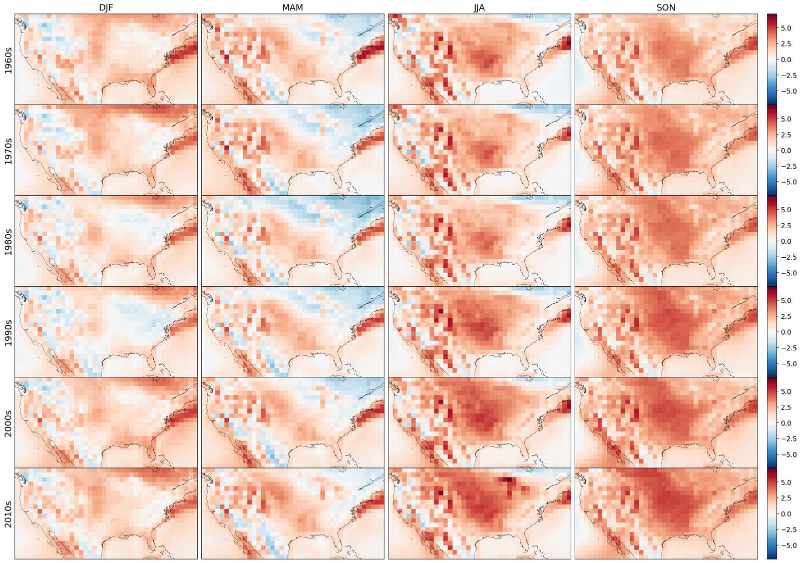
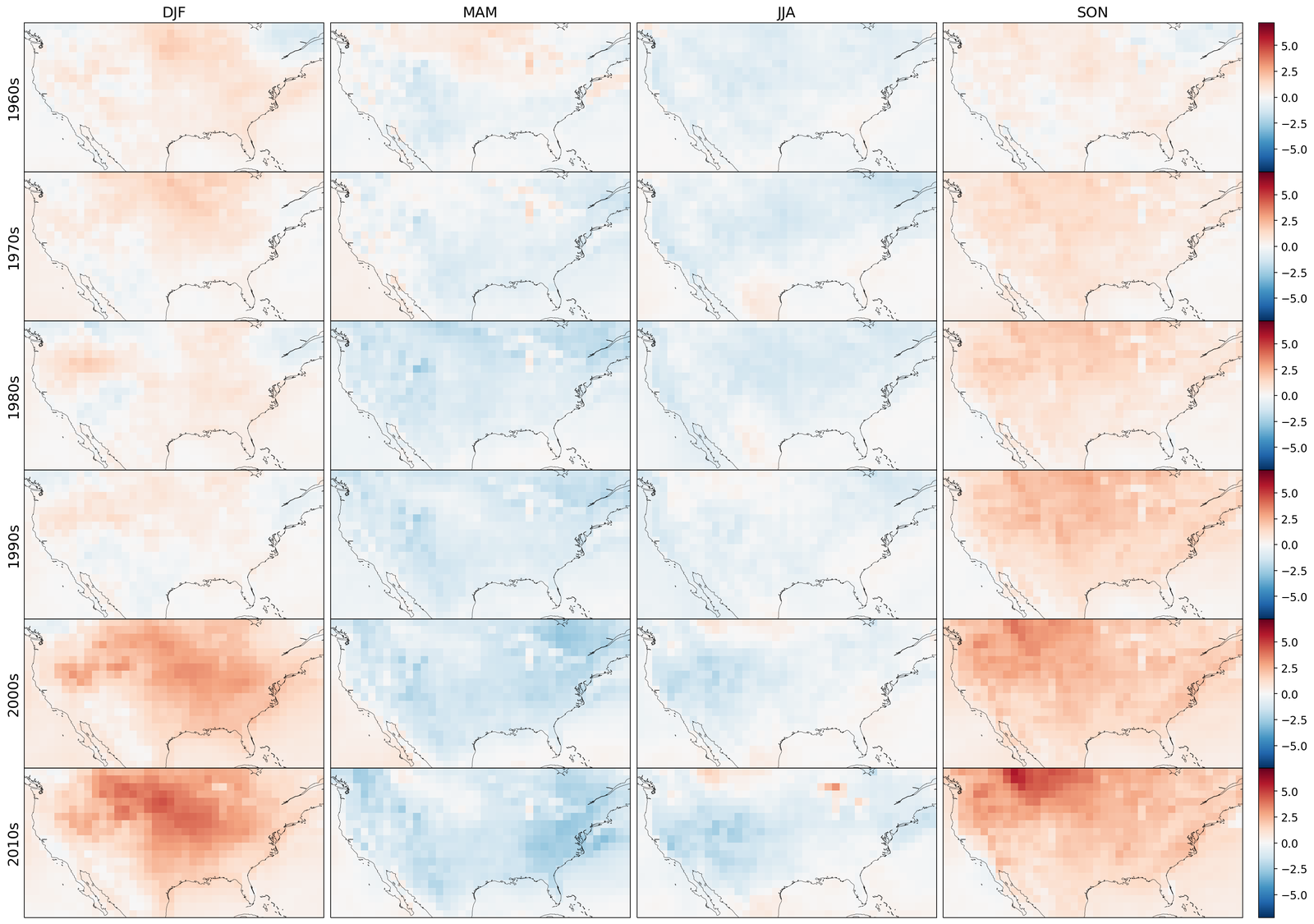
S7.2 Manifold visualization
As our method relies on a manifold alignment idea, we seek to showcase it with the visualization of the manifold projected to a low-dimensional space. Here we use two projection techniques, principal component analysis and t-SNE.
To visualize the manifold alignment process, we use datasets from ERA5, LENS2, and the debiased LENS2 trajectory from 1960 to 2000. We compute the first 3 PCA components of ERA5 data within 1960 and 2020 and project the full dataset onto these components. We compute the density using kernel density estimation for the full 60 years, and we compute the level set of the density, such that most of samples are contained in this manifold. Then, we consider the projection of LENS2 2-meter temperature data for 2020 and its debiased version. The results are summarized in Figure S30, which shows how the debiasing step pushes the LENS2 trajectory back into the high-density sections of the ERA5 manifold.
Additionally, we show a similar example using a t-SNE plot. We compute the t-SNE embedding of 60 years (from 1961 to 2020) of data for ERA5, LENS2, and Reflow-debiased LENS2 (using one member), summarized in Figure S31. This figure shows that LENS2 and ERA5 are mostly separated but have some overlap at the center. We then consider the t-SNE trajectories for 2020 for both LENS2 and its Reflow-debiased version, shown in Figure S31. This reinforces the previous observation: debiasing moves the trajectory from the high-density zone of LENS2 to the high-density region of ERA5, effectively modifying the statistics of LENS2 to match those of ERA5.
Finally, we also plot the level set of the debiased data, along the manifold of ERA5 and LENS2 data, as shown in Figure S32, where we can see that the debiasing effectively transports the LENS2 data to the interior of the high-density region of ERA5.
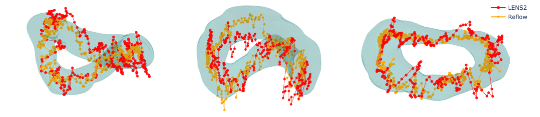
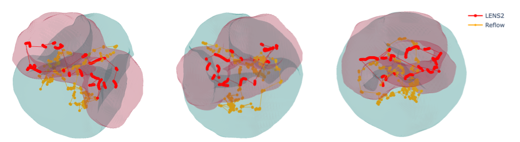
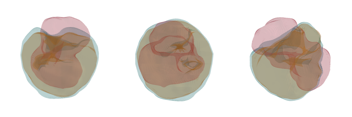
S7.3 Upsampling
We analyze the variability introduced during the upsampling stage of the pipeline, which can be decomposed into three main components: (a) spatial variability, which arises from dividing a single grid point into smaller subgrid points; (b) diurnal variability, resulted from transforming daily mean values into bi-hourly samples; and (c) systematic uncertainty at fixed spatial location and time, reflecting incomplete knowledge of the system.
Figure S33 provides examples for each level of variability, comparing GenBCSR, BCSD and ERA5 reference data. The spatial variability components are notably similar across the models and reference, which is expected given their static nature and strong correlation with topography. The diurnal component, heavily influenced by large-scale conditioning, exhibits less similarity; however, the relative scales of variability remain comparable. Finally, the systematic uncertainty component reveals a key difference between our diffusion-based upsampling approach and the corresponding part of BCSD. Our model exhibits much lower uncertainty induced by large-scale conditioning, whereas BCSD relies on drawing residual samples from historical reference, which are minimally correlated with the conditioning large-scale fields.
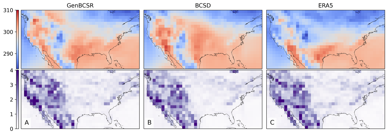
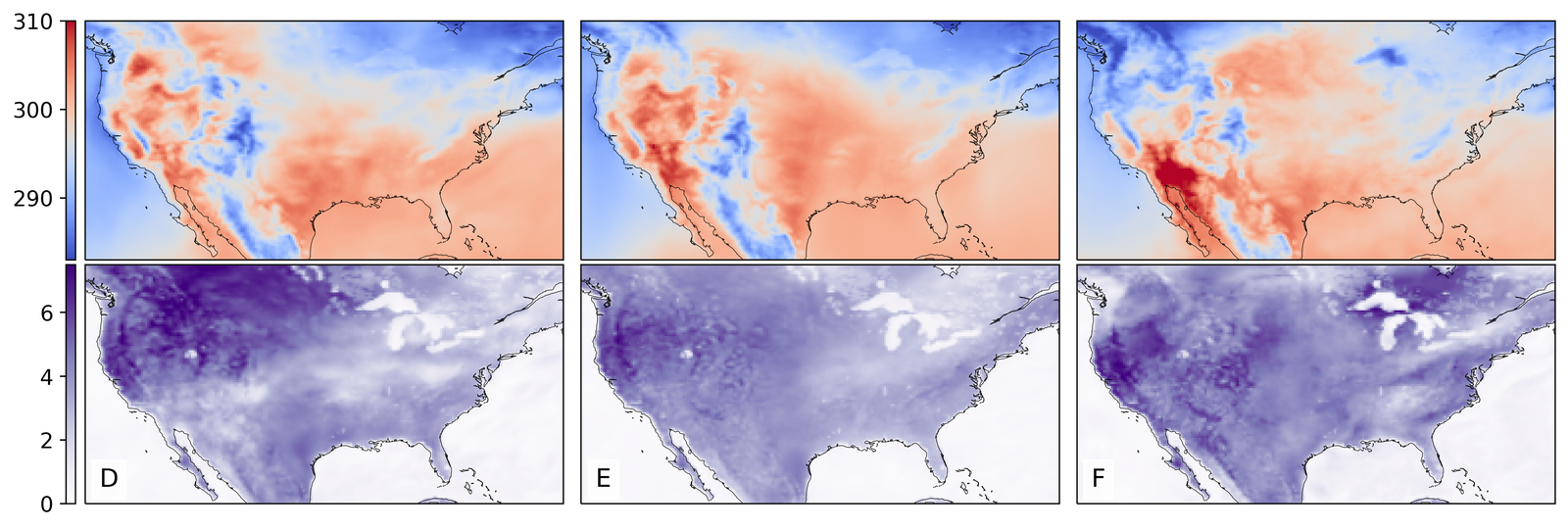
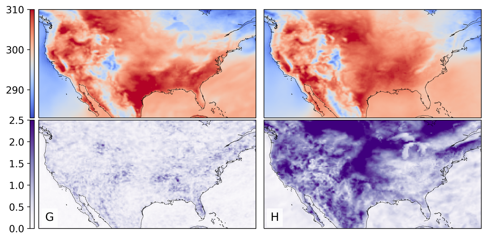
Appendix S8 Downscaling samples
Figure S34, S35 and S36 present generated temperature, wind speed and humidity samples over a contiguous 10-day period, for a fixed ensemble member (cmip6_1301_010).