Statistical inference on partially shape-constrained function-on-scalar linear regression models
Abstract
We consider functional linear regression models where functional outcomes are associated with scalar predictors by coefficient functions with shape constraints, such as monotonicity and convexity, that apply to sub-domains of interest. To validate the partial shape constraints, we propose testing a composite hypothesis of linear functional constraints on regression coefficients. Our approach employs kernel- and spline-based methods within a unified inferential framework, evaluating the statistical significance of the hypothesis by measuring an -distance between constrained and unconstrained model fits. In the theoretical study of large-sample analysis under mild conditions, we show that both methods achieve the standard rate of convergence observed in the nonparametric estimation literature. Through numerical experiments of finite-sample analysis, we demonstrate that the type I error rate keeps the significance level as specified across various scenarios and that the power increases with sample size, confirming the consistency of the test procedure under both estimation methods. Our theoretical and numerical results provide researchers the flexibility to choose a method based on computational preference. The practicality of partial shape-constrained inference is illustrated by two data applications: one involving clinical trials of NeuroBloc in type A-resistant cervical dystonia and the other with the National Institute of Mental Health Schizophrenia Study.
Keywords: Nonparametric estimation, partial shape constraints, shape-constrained kernel least squares, shape-constrained regression spline, testing
1 Introduction
As function-valued data acquisition becomes increasingly common, there has been a significant amount of work devoted to functional regression models to address coefficient function estimation and inferential capabilities [21, 32]. Among them, inference for the function-on-scalar regression (FoSR) model has been making implications in many fields [24] by identifying a dynamic association between response and scalar covariates, varying over the domain. Besides finding the statistical evidence of a non-null covariate effect on response trajectories over the domain, validating the shape of functional regression coefficients, such as monotonicity, convexity, or concavity, over a specific subset of the domain is crucial for domain experts to allow tangible interpretation in practice. Once the functional shape is validated, one may incorporate the corresponding conditions to the model estimates to avoid potential biases. Or, in practical estimation problems, shape restrictions on functional regression coefficients over specific sub-intervals of the domain can be known as prior knowledge.
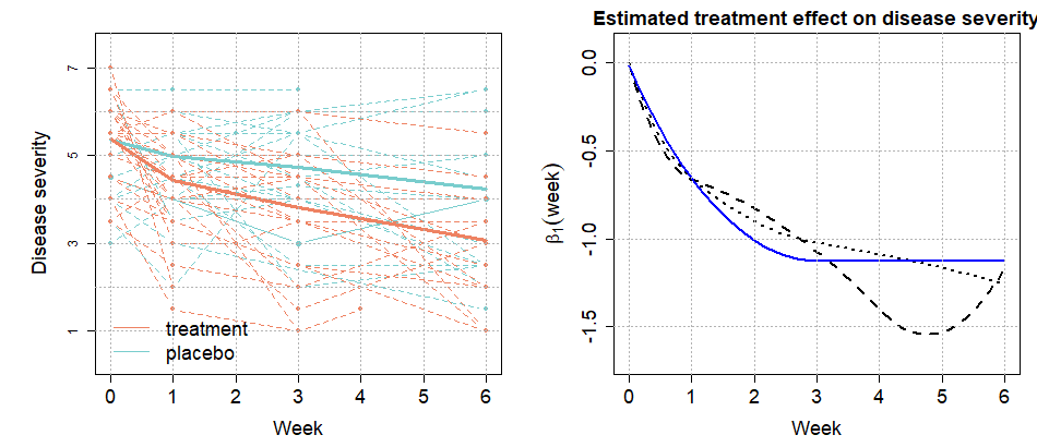
Our motivating example is the functional data analysis approach to demonstrating the treatment efficacy of drug use during the period of clinical trials in the National Institute of Mental Health Schizophrenia Collaborative Study. The previous studies, including [1] and [12], showed a significant continual drop in disease severity for the treatment group, i.e., improving drug efficacy, over weeks through the shape-constraint test on the drug effect coefficient function. While the study design and models are provided in Section 4.2, the left panel of Figure 1 displays the collected longitudinal disease severity measures surveyed from the initial treatment (week 0) to week 6 from randomly selected 30 patients of placebo and treatment cohorts. However, refined conclusions over specific periods can be of practical interest to practitioners, such as when the maximum drug efficacy is achieved or whether we can conclude significant improvement in drug effectiveness even during the later weeks of trials. As we shall see in Section 4.2, our proposed partial inference method concludes the significant monotone decrease in disease severity owing to the drug treatment over weeks 0–3, followed by the consistent duration of such efficacy for the remainder weeks, illustrated with the blue solid line in the right panel of Figure 1. This is somewhat distinct from constrained estimates under the condition of monotone decrease over the entire domain, the conclusion of [12], and unconstrained smooth estimates, which are displayed with the black dotted and dashed lines, respectively.
The recent literature on functional data analysis and its applications also pays attention to shape-restricted estimation and inference in functional regression models. For the inference on shape-constrained regression coefficients, [6] proposed the goodness-of-fit test based on empirical processes projected to the space with shape constraints, while [22] addresses a similar problem under the null hypothesis with linear operator constraints. For estimation, [4] extended the shape-constrained kernel smoothing to the functional and longitudinal data framework, and [12] employed the Bernstein polynomials for shape-constrained estimation in functional regression with one of the data application results from [12] being illustrated in Figure 1. To name of few other applications, in economics, motivated by the pioneering work from Slutsky [31] recognizing the necessity of shape-restricted estimation and inference, [5] elaborated theoretical and application works in econometric research. In public health research, the analysis of growth charts under the monotone increasing shape restrictions has provided a crucial clinical tool for growth screening during infancy, childhood, and adolescence [15] or such growth chart helps health providers assess monotone increasing growth patterns against age-specific percentile curves [9]. The reliability engineering society also paid attention to this topic for bathtub-shaped function estimation in assessing the degradation of system reliability. However, to our best knowledge, inference for partial shape constraints has not been recognized, although such interests can be plausible in practice.
In this study, we propose the inferential tool to validate the partial shape constraints on functional regression coefficients in FoSR, along with two corresponding estimation approaches using kernel-smoothing and spline techniques. Suppose one is interested in the shape constraints on a sub-interval , where collected response trajectories span . Under the existing tools for shape-constrained inference, one might consider using a part of functional observations restricted on and apply the standard testing procedure. However, such an approach will cause a significant drop in sample sizes in the case of a bounded number of measurements on response trajectories, which is common in longitudinal studies, including our motivating example illustrated in Figure 1. The situation becomes much worse depending on the length of or the sparsity of evaluation grids on it. Consequently, this naive approach would result in a severe deterioration in the power. To prevent this, we propose to borrow information from observations over the entire domain to perform the inference even for testing focused on specific subsets of the domain. It indeed prevents the significant drop in the power of the test while keeping the desirable level of type-I error, as demonstrated in the simulation studies of Section 3. The other contribution of our paper is in developing two partial shape-constrained regression estimators in parallel using the most widely used nonparametric smoothing techniques, kernel-smoothing and smoothing splines. The proposed unified testing tool applicable to both estimates would provide practical flexibility in a real application. We additionally derive asymptotic behaviors of the regression coefficient estimators with embedded partial shape constraints.
The article is organized as follows. Section 2 presents the proposed method and results of the study. We introduce the partially shape-constrained FoSR models in Section 2.1. The estimation methods and theoretical findings are provided in Sections 2.2 and 2.3 that cover the kernel and spline estimators, respectively. In Section 2.4, we establish a unified inferential procedure for testing the partial shape constraints, encompassing kernel and spline approaches. Simulation results are reported in Section 3, and data applications are illustrated with two examples in Section 4. Technical details and proofs are provided in Supplementary Material.
2 Methodology and Theory
2.1 Testing partial shape constraints in FoSR models
Let be the functional response coupled with a vector covariate as
| (2.1) |
independently for , where is a vector coefficient function and is a mean-zero stochastic process that models the regression error uncorrelated with , i.e., . We assume that are linearly independent with positive probability, which allows the design matrix to include the intercept, e.g., for all , depending on the inferential interest. Despite the generality of the functional model (2.1), it is practically infeasible to observe the functional outcomes as the infinite-dimensional objects, and we assume that discrete evaluations with are only accessible for , where is a random sample of with a probability density function on . Here, is an independent random integer that may or may not depend on the sample size . More detailed conditions on required for kernel and regression spline methods are provided in the Supplementary Material S.1 and S.2. We denote the finite random sample as .
Suppose we test the functional shape of on a pre-specified sub-interval for with . The null hypothesis “” consists of individual hypotheses
| (2.2) |
for . For example, if we hypothesize that is monotone increasing on , we read (2.2) as “.” Similarly, if one tests a partial convexity hypothesis, (2.2) can also be written as “.” In this paper, monotone and convex hypotheses will mainly be exemplified, yet one can extend our framework to general shape constraints, similarly as covered by many others in the literature [17, 18, 27, 28, 20, 25].
We then propose to reject the null hypothesis if the test statistic
| (2.3) | ||||
is significantly large, where and denote the estimates of coefficient function under the null hypothesis and its general alternative , respectively. While this is partly motivated by [22], a goodness-of-fit based test statistic for validating functional constraints on via linear operator, similar types of the -based test statistics were frequently employed in the literature for testing the nullity of functional difference for general scope [30, 36, 35]. Indeed, our proposed method corresponds to the global shape constraints if one sets . The following Sections 2.2 and 2.3 elaborate on how to obtain under kernel-smoothing and spline-smoothing approaches, respectively. Based on those estimators, we present a bootstrap test procedure in Section 2.4.
2.2 Estimation: Shape-constrained kernel-weighted least squares
We assume that the vector coefficient is as smooth as it allows local linear approximation for near , where denotes the gradient of . The local linear kernel estimator of is given by the unconstrained minimizer of the following objective function.
| (2.4) | ||||
where with a probability density function and a bandwidth , is the local smoothing design, and with of and the Kronecker product of the covarite design for local linear smoothing.
Proposition 2.2.1.
For each , let be the matrix, where is the true vector coefficient function such that exists and is continuous. Suppose conditions – in Supplementray Material S.1 hold. Then, we have
| (2.5) |
The implication of conditions – are provided in Supplementary Material S.1. It is worth mentioning that Proposition 2.2.1 is valid even if only a few longitudinal observations are available for some subjects. For example, it is common in observational studies that dense observations of functional responses for some subjects may not be available regardless of the sample size , i.e., the minimum number of longitudinal observations is bounded. Therefore, the technical condition on in is not a restriction because we do not require as .
Remark 1.
For the shape-constrained estimation of under , we extend the kernel-weighted least squares for nonparametric regression with scalar responses [34], where side conditions are empirically examined over a fine grid with so that satisfies the null hypothesis (2.2) over for each . Specifically, if we consider “,” we propose to substitute
| (2.6) |
Similarly, we empirically validate the partial hypothesis “” as
| (2.7) |
To define the shape-constrained kernel-weighted least squares for the function-on-scalar regression model (2.1) under the empirical null hypothesis on the grid , we note that
| (2.8) | ||||
where is the unconstrained residual of fitting and with . To get (2.8), we used the fact that the unconstrained estimator solves the estimating equation , or equivalently , where denotes the zero vector in . Noting that the minimization of only depends on the first term of (2.8) given the unconstrained estimator , we propose the constrained optimization problem as follows.
| (2.9) | ||||
where and are the -vector and -matrix of zeros, respectively, and is the linear constraint matrix associated with the individual hypothesis . For the monotone increasing hypothesis (2.6), we set , where is the unit vector with only at its -th coordinate and is defined as
| (2.14) |
Similarly, for the convexity hypothesis (2.7), we set we set , where are defined as
| (2.15) | ||||
and . This illustrates that the constrained estimates can be obtained by the standard quadratic programming with linear constraints.
Remark 2.
Suppose we hypothesize “,” where and may or may not overlap. Then, the side conditions corresponding to the null hypothesis can also be examined by imposing both linear constraint matrices and .
Theorem 2.2.2.
Theorem 2.2.2 indicates that the shape-constrained kernel least square estimator achieves the same rate of convergence as the unconstrained estimator under the null hypothesis. Moreover, suppose the empirical distribution of converges to the uniform distribution on . Then, it can be verified that similarly to Remark 1.
2.3 Estimation: Shape-constrained regression spline
We now consider fitting the functional regression model by means of spline functions for smooth, flexible, and parsimonious estimation of coefficient functions. Let , denote spline basis functions defined over for a given sequence of knots, then we express , where denotes the basis coefficients. Under the shape constraints on over , we can still employ the regression spline approach based on chosen basis functions, such as -splines [23], -splines [18] or general -splines, with corresponding constraints assigned on a subset of basis coefficients . While we focus on partially constrained estimation based on - or - splines in this section, estimation via -splines is also discussed in the Supplementary Material S.6.
[23] first introduced -splines for curve estimation under the monotonicity restriction over the entire domain. As illustrated in the left panel of Figure 2, -spline basis functions are piece-wise quadratic, and at each of the knots indicated by dotted vertical lines, there is exactly one basis function with a non-zero slope. Thus, a monotone increasing (decreasing) spline function can be constructed as a non-negative (non-positive) linear combination of -spline basis functions. For readers interested in generating process of -splines, we refer [23] on how piece-wise quadratic -splines are formed from nonnegative -spline family. Then, if the specific aim is on assigning, for example, monotone increasing restriction over a subset of the domain , non-negative coefficients condition should apply to a subset of for which corresponding -spline display positive slopes within the range of .
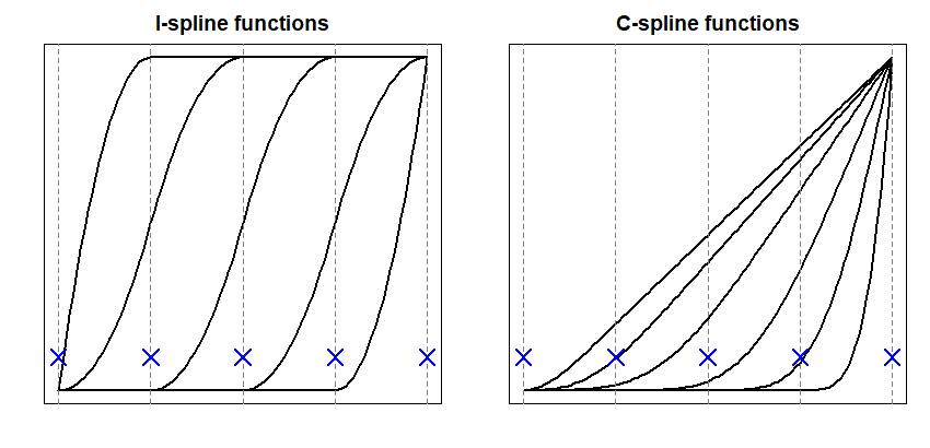
Next, in terms of convexity constraints, [18] proposed -splines by integrating -splines. As shown in the right panel of Figure 2, -splines form convex and piece-wise cubic functions with non-zero second derivatives at each knot, implying that a linear combination of -splines with non-negative (non-positive) basis coefficients ensures the convexity (concavity) of the function estimator. See Section 2 of [18] for details. Similarly, for the convexity constraints over sub-interval(s) , we can impose non-negative restrictions to basis coefficients corresponding to splines showing positive second derivates features within .
We now apply the shape-restricted spline function technique to the functional regression model framework to estimate functional coefficients under (2.2). Although methodological or theoretical developments are general to other shape constraints, such as convexity or monotone convexity, we elaborate on the estimation under the monotonicity restriction below and refer to remarks for other restrictions. Let , , denote piece-wise quadratic -spline basis functions under a given knot sequence, employed to fit , . Especially for partially constrained coefficients , the knot sequence should include lower and upper boundaries of . For the case of multiple disjoint sub-intervals form of , all boundaries should be a part of the knot sequence. We then estimate the functional regression coefficients by minimizing the following objective function with respect to non-negative conditions assigning on a subset of basis coefficients depending on the set and as,
| (2.17) | ||||
where indicates the intercept function, i.e., , so that represents the location of monotonicity functions of , the dimensionality of splines is determined by the number of knots chosen to approximate , the set from (2.2) includes indices which coefficients are constrained in , and the set is defined as .
To obtain shape-restricted , we first write our regression problem associated with (2.17) as below. We elaborate for the case of regular evaluation grids, , for , and for representation simplicity, but having different or does not affect methodological developments. Let for , then
| (2.18) |
under for certain specified in (2.17), where denotes a basis matrix having its -th row consisting of for . Then, the coefficient estimation is associated with finding the projection of -dimensional onto the space spanned by columns of with corresponding constraints on , where denotes the design matrix. By letting , for , denote the set of column vectors on and represent the linear space spanned by a given set of vectors, we separate , , a set of column vectors associated with basis coefficients with no non-negativity constraint, and define indicating the linear space spanned by them. We then further obtain a set of generating vectors, denoted as for satisfying , that are orthogonal to . That is, , for , where indicates a projection operator, such as the Gram-Schmidt process. By extending [18], we can characterize the constrained set as
| (2.19) |
Then the projection of to can be fulfilled by projecting it onto the set of nonnegative linear combinations of , , called as constraint cone, and onto the , separately. We refer to Section 2 of [18] for readers interested in more comprehensive descriptions under a nonparametric regression setting. Owing to the fact that the constraint set is a closed convex polyhedral cone in , the projection is unique, and we employ the cone projection algorithm of [19] to find a solution, available as the function qprog or coneA in the R package coneproj. We note that the unconstrained estimates can be calculated by the least square estimates of under (2.18).
Next, we investigate rates of convergence for estimated functional coefficients under the constraints. Let denote the number of knots to fit growing with , is the order of the spline, and be the norm of a square-integrable function . Under Conditions –, deferred in Supplementary Material S.2, and for , Theorem 2 of [14] and Theorem 6.25 of [26] imply the consistency of unconstrained written as, , Next, we show the consistency of the constrained estimators by adding the condition (S7) specified in Supplementary Material.
Theorem 2.3.1.
When shape constraints assigned to is true in , , and conditions – are satisfied, the constrained estimator attains the same rate as the unconstrained estimator.
where its minimum rate is achieved when .
Remark 3 (Convexity shape constraints).
When the convexity constraint is considered in (2.2) instead of monotonicity, we employ -splines and express the coefficient function in the objective function (2.17) as where denotes the intercept function, is the identity function, i.e., , and denotes -splines under a given sequence of knots. The first two terms without constraints on and determine the first-order behaviors of functional coefficients. Then, we assign constraints , for , where and with the set defined as . The non-negativity constraints on basis coefficients associated with having positive second derivatives within ensures the convexity of functional estimates over . For concavity constraint, we apply the same framework but with non-positivity constraints on a chosen set of . In this way, we can consider general with various types of shape constraints on over , for .
2.4 Test procedure
We employ a resampling method to assess the statistical significance of the observed given a random sample . We note that resampling functional observations , say , is not straightforward because should inherit the joint distribution of with within-subject heteroscedasticity. In literature, the wild bootstrap method [33, 13, 16] has been extensively investigated that can effectively handle the heteroscedasticity, and there have been many advances for handling dependent data [3, 7, 29, 11]. In this study, we use the wild bootstrap procedure as described in Algorithm 1, which can be regarded as the wild bootstrap for clustered data [3, 7].
Once bootstrap samples are independently generated, we calculate the shape-constrained and unconstrained estimates and , and calculate the test statistic , for each . These bootstrap test statistics are compared to the original test statistic to determine the bootstrap -value, . Then, we reject the null hypothesis if , and retain otherwise at the significance level . Our numerical study (Section 3) demonstrates that the proposed test procedure fulfills consistency in the sense that the type I error rate meets the significance level as specified and that the power of the test increases as sample size increases.
3 Simulation Study
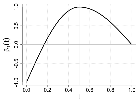
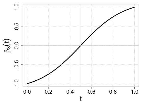
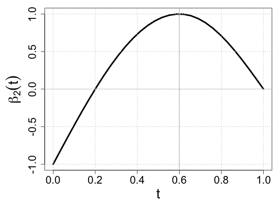
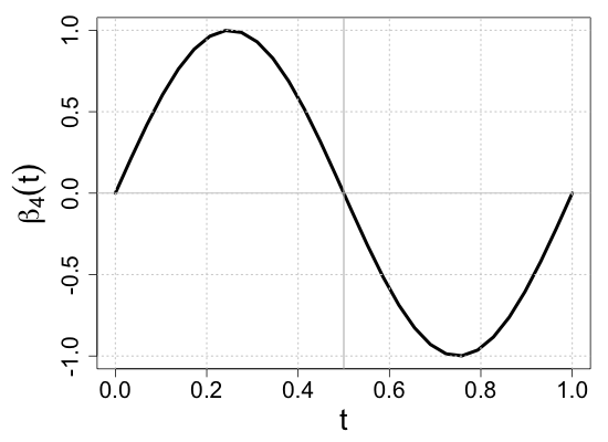
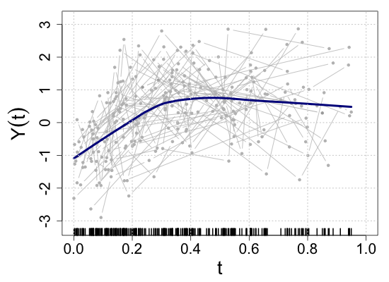
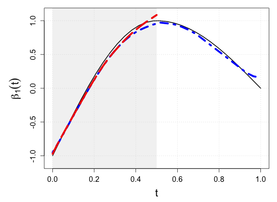
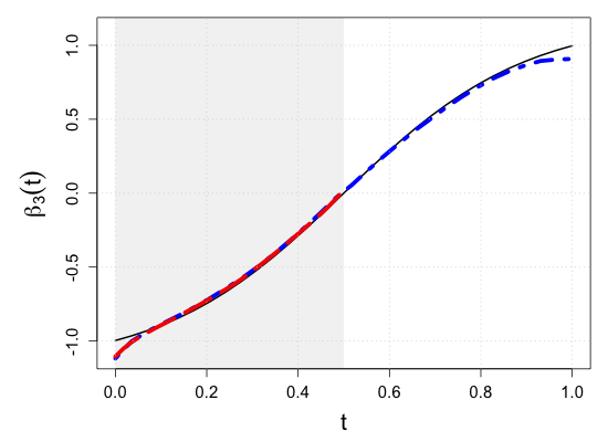
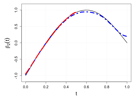
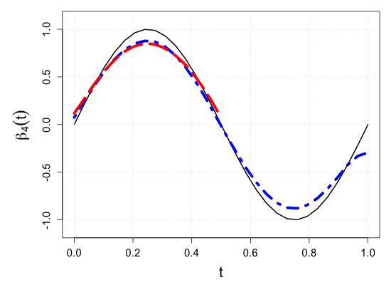
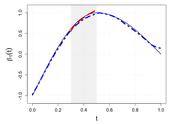
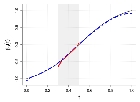
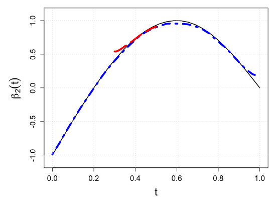
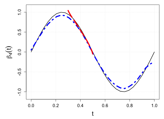
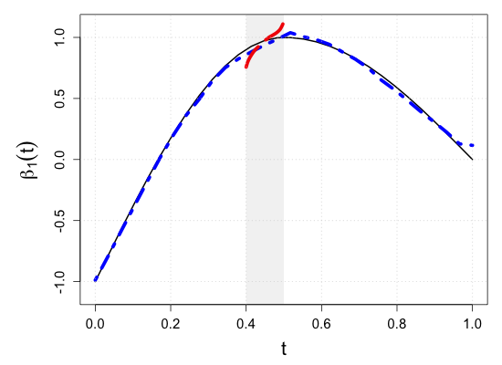
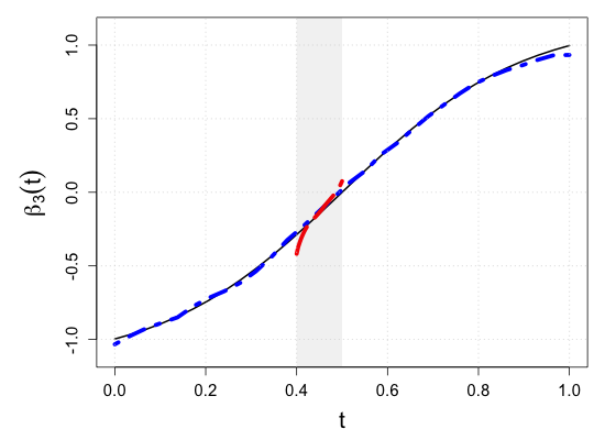
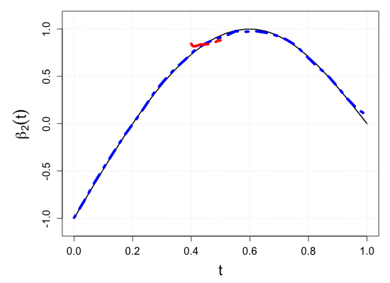
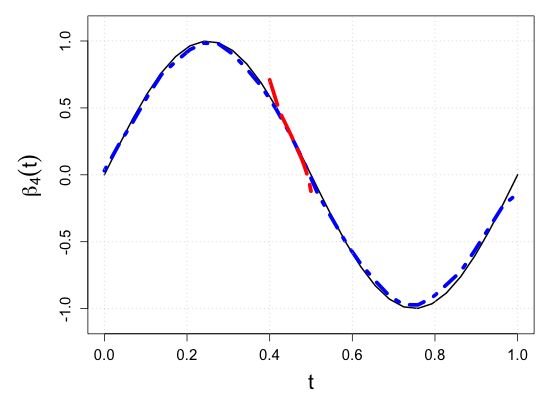
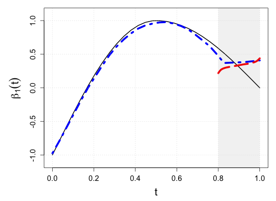
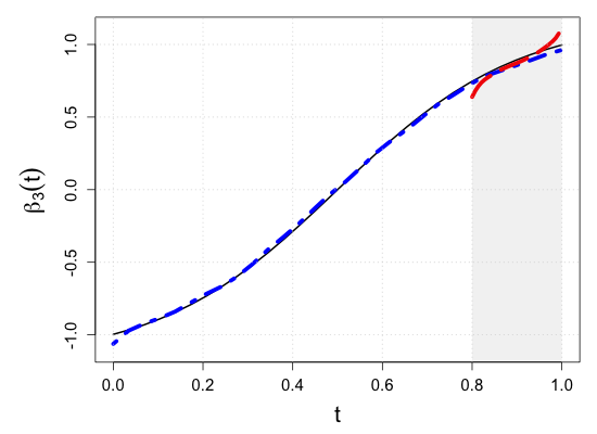
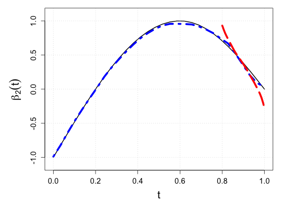
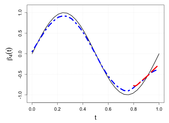
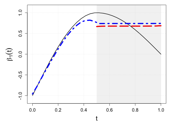
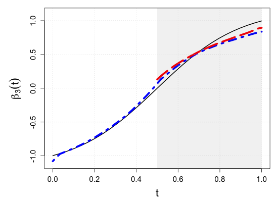
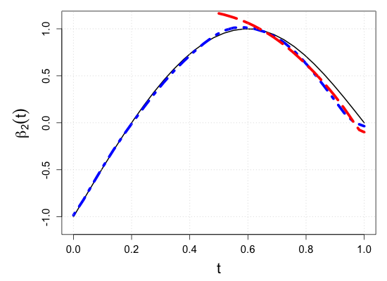
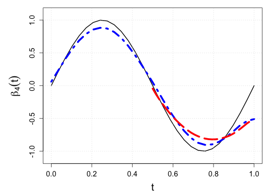
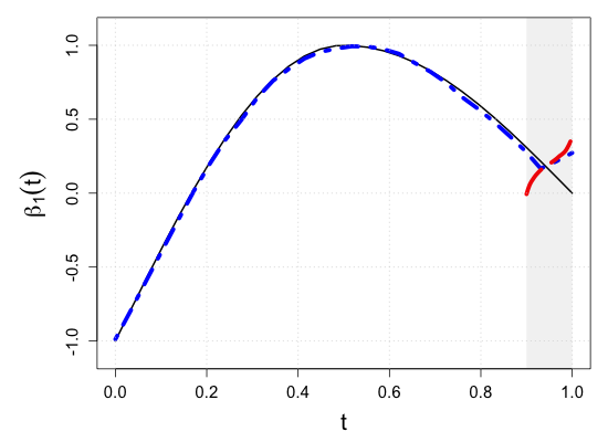
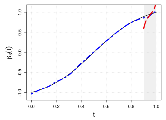
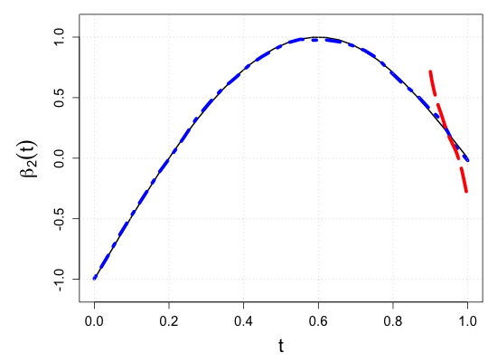
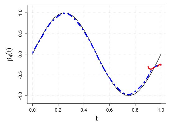
We demonstrate the finite-sample performance of the proposed methods with numerical simulations. As described in Section 2, functional observations are assumed to be only partially available in our simulation study. Specifically, we first generate subject-specific evaluation points independently drawn from , which is a right-skewed distribution on . Here, is a uniform random integer on , representing the bounded number of sparse and irregular observations. Then, longitudinal observations of each functional response are generated by the model (2.1) associated with four functional coefficients depicted in Figure 3(a), where the random vector of scalar covariates is given by with independent uniform random variables on . This makes the four components correlated. Moreover, to introduce the within-subject dependency of longitudinal observations, we set the functional noise as , where has a multivariate normal distribution with mean zero and and is a Gaussian white noise process with mean zero and . Then, we have a random sample of size .
We consider testing a composite null hypothesis
| (3.1) |
where is a pre-specified sub-interval to which the partial shape constraints of interest apply. This setup is intended to mock up one of the common situations in longitudinal studies such that patients drop out of the study or transfer to other clinics. For example, as the vertical rugs show that evaluation points are right-skewed in Figure 3(b), fewer observations are available near . Still, verifying the partial shape constraints on regression coefficient functions near can be of inferential interest. For a systematic assessment of the numerical experiments, we consider ten simulation scenarios of the sub-interval , , , , , , , , , and . With the graphical illustration of the true regression coefficient functions in Figure 3(a), we note that the null hypothesis (3.1) is true if , and false otherwise.
To demonstrate the consistency of the proposed method subject to the different scenarios of , we evaluate the power of the test by the Monte Carlo approximation as
| (3.2) |
at the significance level , where is the -value obtained in each -th Monte Carlo repetition under the null hypothesis (2.2). Since gives the empirical level of the test, we can validate how much the proposed test keeps the test level as specified with different significance levels. Under the general alternative, corresponds to the empirical power of the test, and we can examine how fast approaches 1 as the sample size increases.
Besides the consistency of the partially shape-constrained inference, we evaluate the consistency of estimation with the integrated squared bias (ISB) and the integrated variance (IVar),
| (3.3) |
where is the average of the shape-constrained estimates obtained from the repeated Monte Carlo experiments. In (3.3), we normalize the ISB and IVar by to easily compare the trend of numerical performances obtained from the different lengths of sub-intervals. Combining the above (3.2) and (3.3), we can assess the sensitivity and specificity of the proposed test procedure subject to the location and length of the sub-interval. We mainly report the simulation results obtained with and , but our background simulation study gave the same lessons with larger and . We refer the readers to Section S.3 of the Supplementary Materials for the implementation details, including the bandwidth and knots selection for the shape-constrained kernel smoothing and regression spline, respectively.
We also consider a sub-cohort analysis for a comparative study, shedding light on another essential feature of the proposed method. As mentioned in the Introduction section, one may argue that it is more appropriate to simply treat (3.1) as global shape constraints “ and are globally monotone increasing” under the model (2.1) restricted to . In this concern, we conduct the sub-cohort analysis using the same inferential procedure as the proposed method but only utilizing the partial data , where . In contrast to the sub-cohort analysis, we call our proposed method the “full cohort” analysis since it uses all available observations in for estimation regardless of . As seen below, our simulation result indicates that the sub-cohort analysis suffers from a significant loss of information. The more is located in the second half of the domain, the smaller the statistical power one may expect. The situation becomes much worse depending on the length of and the sparsity of functional evaluations on it. Through our simulation study, we also demonstrate that the proposed test procedure is robust against the location of sub-intervals.
| Sample size | Dataset | Criterion | and are monotone increasing on . | |||
|---|---|---|---|---|---|---|
| Kernel least squares | Spline regression | |||||
| Full data | ||||||
| Partial data | ||||||
| restricted to | ||||||
| Full data | ||||||
| Partial data | ||||||
| restricted to | ||||||
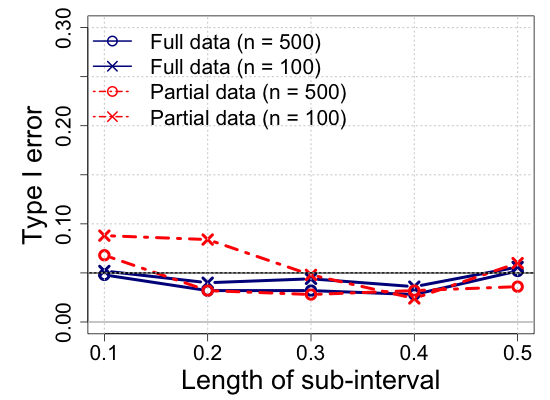
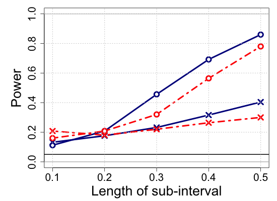
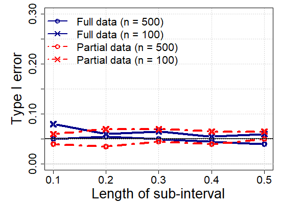
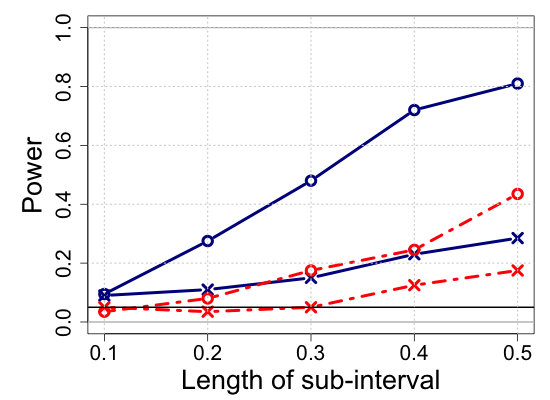
We report the simulation results in Table 1 and Figure 4, highlighting the main lessons we obtained in the power analysis and estimation performance. The additional simulation results are provided in Section S.7 of the Supplementary Materials. The proposed partially shape-constrained inference (full cohort analysis) outperforms the sub-cohort analysis with the global shape constraints. Specifically, Table 1 shows that both the kernel and spline methods yield consistent estimates in the sense that ISB and IVar decrease as the sample size increases, which is well-aligned with the large sample properties we investigated in Section 2. Figure 4 shows that the proposed test procedure consistently meets the level of the test as specified () across different scenarios varying with the length of sub-intervals from to .
We note that the proposed method keeps the significance level under the null hypothesis and generally attains a greater power under the general alternative, while the sub-cohort analysis often violates the pre-specified level of the test under the null hypothesis. For the sub-interval , the sub-cohort analysis appears more sensitive to the general alternative than the full cohort analysis. However, as shown in Figure 1(b) in the Supplementary Materials, the shape-constrained estimates of the sub-cohort analysis suffer from significant bias due to the low sample size with . A similar issue arises with the sub-interval , where the sub-cohort analysis exhibits a higher type I error rate compared to the full cohort analysis. Therefore, we do not recommend using the sub-cohort analysis for verifying partial shape constraints over short sub-intervals.
4 Real Data Applications
We illustrate the application of shape-constrained inference to two datasets from clinical trials and demonstrate how we figure out treatment efficacy over time. The proposed tools help summarize dynamic efficacy patterns so that practitioners better understand when the maximum treatment effect is achieved and decide the appropriate treatment frequencies. Compared to existing studies making such conclusions relying on visualization of estimated regression coefficient functions or based on inference over the entire domain, our method enables providing statistical evidence on refined conclusions on any sub-intervals of interest. Although we illustrate examples from clinical trials, the proposed tool can be applied to any field with similar interests.
4.1 Application 1: Cervical Dystonia Dataset
Cervical dystonia is a painful neurological condition that causes the head to twist or turn to one side because of involuntary muscle contractions in the neck. Although this rare disorder can occur at any age, it most often occurs in middle-aged people, women more than men. The dataset is collected from a randomized placebo-controlled trial of botulinum toxin (botox) B, where 109 participants across 9 sites were assigned to placebo (36 subjects), 5000 units of botox B (36 subjects), or 10,000 units of botox B (37 subjects), injected into the affected muscle to partially paralyze it and make it relax. The response variable is the score on the Toronto Western Spasmodic Torticollis Rating Scale (TWSTRS), measuring the severity, pain, and disability of cervical dystonia, where higher scores mean more impairment on a 0-87 scale. The TWSTRS is administered at baseline (week 0) and at weeks 2, 4, 8, 12, and 16 thereafter. This study was originally conducted by [2], and 96.5% of subjects were followed up at designated weeks, on average. Besides, the dataset contains information on the age and sex of the subjects. The data is available in R through the package ‘medicaldata’ (https://github.com/higgi13425/medicaldata). While [2] or [8] focus on demonstrating the efficacy of botox B in cervical dystonia during weeks of clinical trial under longitudinal models, our application aims to assess the pattern of drug efficacy over weeks by applying shape-constrained inference on various sub-intervals and investigate when the maximum efficacy is achieved. To do this, we introduce the indicator variables , where if the drug is assigned to th subject, and , otherwise. We then consider the following regression model
| (4.1) |
| Hypothesis | -values | |
|---|---|---|
| Kernel-based | Spline-based | |
| is monotone decreasing on | 0.36 | 0.45 |
| is monotone increasing on | 0.03 | 0.02 |
| is monotone decreasing on | 0.07 | 0.01 |
| is monotone increasing on | 0.84 | 0.48 |
Table 2 contains the results of the monotonicity tests, is monotone decreasing (increasing) over two sub-intervals, and , from the kernel- and spline-based tests using bootstrap size . The spline-based approach specifically adopts piece-wise quadratic -spline basis functions with one internal knot located at , determined by cross-validation as detailed in Supplementary Material S.3. To estimate with shape restriction over or , we locate one additional knot at only for to present desired shape under given boundaries. The kernel-based results are obtained from estimates based on optimal bandwidth with the detailed selection criteria discussed in Supplementary Material. Then, we observe that both kernel- and spline-based tests conclude the significant decreasing from weeks 0 to 4 by rejecting is monotone increasing on , but declare an increasing pattern observed from weeks 4 to 16 by rejecting is monotone decreasing on under the significant level 0.1. This conclusion implies the improving efficacy of botox B during the first 4 weeks, but diminishing effectiveness after then. This finding becomes more convincing through consistent conclusions regardless of the choice of shape constraints on null hypotheses, either monotone decreasing or increasing, or choice of estimation methods.
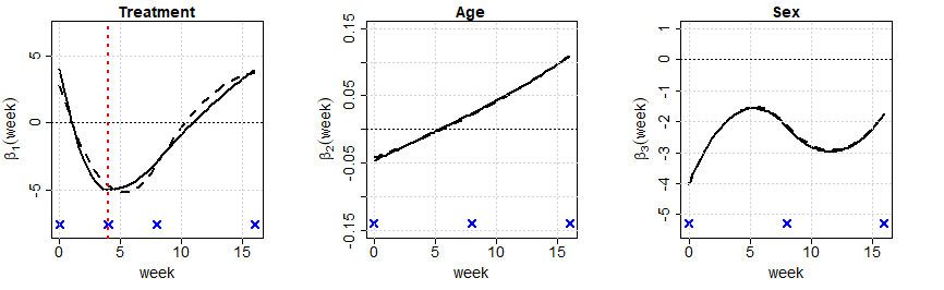
Figure 5 displays the estimated functional coefficients under spline estimates with the chosen optimal selection of knots in each panel. Following the inferential conclusion on treatment effect, is estimated under the decreasing constraint over weeks from 0 to 4 and under the increasing constraint during weeks from 4 to 16. The unconstrained and constrained models are fitted using the same knots, but one extra knot at week 4 is added to fit due to shape constraint changing at week 4. We observe the positive coefficients at week 0, presumably due to a slight bias from the random assignment in the trial, with the mean of response scores from placebo and treatment groups calculated as 43.5 and 46.7, respectively, at baseline (week 0). Although patients in the treatment group show slightly higher scores at the beginning, the decreasing trend in the first four weeks, i.e., improving efficacy, is clear from the estimated function. After 4 weeks, the degree of effectiveness weakens, and at week 16, there is no more treatment effect by returning to the status that we observed from week 0. While we find a precise fit for under shape constraints, remainder regression coefficient estimates for age and sex, and , show similar fits with or without constraints on . In addition to the conclusion on overall treatment efficacy as in [2], we could make a comprehensive summary of treatment efficacy based on refined conclusions over sub-intervals of interest, and it further helps precise estimation.
4.2 Application 2: Mental Health Schizophrenia Collaborative Study
We next implement the proposed method on the data from the National Institute of Mental Health Schizophrenia Collaborative Study, where 437 patients were randomized to receive either a placebo or anti-psychotic drug, followed by longitudinal monitoring of individuals. [1] and [12] already analyzed this data to assess the efficacy of the drug using Item 79 ‘Severity of Illness,’ the Inpatient Multidimensional Psychiatric Scale (IMPS) ranging from 1 (normal, not ill at all) to 7 (among the most extremely ill), evaluated at weeks 0, 1, 3, 6 under the protocol along with additional measurements for some patients made at weeks 2, 4, 5. There were a total of 108 and 329 patients in the placebo and treatment groups, respectively, with an average of among them collected during weeks of protocol and % collected during other weeks. The data is available in R (Package ‘mixor’). As in [1] and [12], we consider the regression model , , where denotes the illness severity measurement of th subject at week , and represents the effect of drug treatment over weeks with the indicator dummy variable ; for individuals assigned in treatment group. As mentioned in the Introduction, although [1] and [12] demonstrated its improving effectiveness over the entire domain, from week 0 to 6, through conclusion on significant decreasing using their inferential tools under shape-constrained estimation, respectively, we are furthermore interested in the efficacy dynamics in later weeks by applying sub-interval tests, similar to what we conducted in Section 4.1. This is motivated by Figure 4 of [1], displaying a clear decreasing trend on estimated with narrow confidence over weeks 0 - 3, but flattening out phase afterward with widening confidence intervals. By applying sub-interval tests over weeks 0 to 3 and weeks 3 to 6, we examine patterns in efficacy beyond the overall drug effectiveness.
| Hypothesis | -values | |
|---|---|---|
| Kernel-based | Spline-based | |
| is monotone decreasing on | 0.71 | 0.26 |
| is monotone increasing on | 0.05 | 0.00 |
| is monotone decreasing on | 0.65 | 0.15 |
| is monotone increasing on | 0.62 | 0.11 |
Table 3 provides -values from is monotone increasing (decreasing) over with bootstrap size . The optimal bandwidth for kernel estimates is set as , and for spline estimates, we adopt piece-wise -splines with two internal knots located at and 4. Both kernel- and spline-based tests conclude the significant decreasing during weeks 0 - 3, supported by -values less than or equal to significance level from the null hypothesis of monotone increasing. Consistently, the null hypothesis for monotone decrasing over weeks 0 -3 is not rejected from both tests. However, sub-interval tests over weeks 3 - 6 conclude that there is not enough statistical evidence to reject both the monotone increasing and decreasing trends. Thus, we conclude the constant level of maintained over this period, implying the maximum drug efficacy achieved at week 3 and the duration of such degree of effectiveness until the end of the experiment. The estimated drug effect is illustrated in Figure 1 with the estimates with no constraints and with decreasing constraints over the entire domain. As discussed in the Section 1, the latter fit is the inferential finding from [1] and [12].
References
- [1] M. Ahkim, G. I., and V. A. Shape testing in varying coefficient models. Test, 26:429–450, 2017.
- [2] A. Brashear, M. Lew, D. Dykstra, C. Comella, S. Factor, R. Rodnitzky, R. Trosch, C. Singer, M. Brin, and J. Murray. Safety and efficacy of NeuroBloc (botulinum toxin type B) in type A–responsive cervical dystonia. Neurology, 53(7):1439–1439, 1999.
- [3] A. C. Cameron, J. B. Gelbach, and D. L. Miller. Bootstrap-based improvements for inference with clustered errors. The review of economics and statistics, 90(3):414–427, 2008.
- [4] Z. Chen, Q. Gao, B. Fu, and H. Zhu. Monotone nonparametric regression for functional/longitudinal data. Statistica Sinica, 29(4):2229–2249, 2019.
- [5] D. Chetverikov, A. Santos, and A. M. Shaikh. The econometrics of shape restrictions. Annual Review of Economics, 10(1):31–63, 2018.
- [6] J. A. Cuesta-Albertos, E. García-Portugués, M. Febrero-Bande, and W. González-Manteiga. Goodness-of-fit tests for the functional linear model based on randomly projected empirical processes. The Annals of Statistics, 47(1):439–467, 2019.
- [7] R. Davidson and E. Flachaire. The wild bootstrap, tamed at last. Journal of Econometrics, 146(1):162–169, 2008.
- [8] C. S. Davis. Statistical Methods for the Analysis of Repeated Measurements. Springer Texts in Statistics. New York, NY: Springer Nature, 1 edition, 2003.
- [9] L. Dümbgen. Shape-constrained statistical inference. Annual Review of Statistics and Its Application, 11, 2024.
- [10] Y. Fan and E. Guerre. Multivariate local polynomial estimators: Uniform boundary properties and asymptotic linear representation. In Essays in Honor of Aman Ullah, volume 36, pages 489–537. Emerald Group Publishing Limited, 2016.
- [11] S. Friedrich, F. Konietschke, and M. Pauly. A wild bootstrap approach for nonparametric repeated measurements. Computational Statistics & Data Analysis, 113:38–52, 2017.
- [12] R. Ghosal, S. Ghosh, J. Urbanek, J. A. Schrack, and V. Zipunnikov. Shape-constrained estimation in functional regression with bernstein polynomials. Computational Statistics & Data Analysis, 178:107614, 2023.
- [13] W. Härdle and E. Mammen. Bootstrap methods in nonparametric regression. In Nonparametric functional estimation and related topics, pages 111–123. Springer, 1991.
- [14] J. Z. Huang, C. . Wu, and L. Zhou. Polynomial spline estimation and inference for varying coefficient models with longitudinal data. Statistica Sinica, 14(3):763–788, 2004.
- [15] R. J. Kuczmarski. 2000 CDC growth charts for the United States: Methods and development. Number 246. Department of Health and Human Services, Centers for Disease Control and Prevention, National Center for Health Statistics, 2002.
- [16] E. Mammen. Bootstrap and wild bootstrap for high dimensional linear models. The annals of statistics, 21(1):255–285, 1993.
- [17] E. Mammen, J. S. Marron, B. A. Turlach, and M. P. Wand. A General Projection Framework for Constrained Smoothing. Statistical Science, 16(3):232 – 248, 2001.
- [18] M. C. Meyer. Inference using shape-restricted regression splines. The Annals of Applied Statistics, 2(3):1013–1033, 2008.
- [19] M. C. Meyer. A simple new algorithm for quadratic programming with applications in statistics. Communications in Statistics - Simulation and Computation, 42(5):1126–1139, 2013.
- [20] M. C. Meyer. A framework for estimation and inference in generalized additive models with shape and order restrictions. Statistical Science, 33(4):595–614, 2018.
- [21] J. S. Morris. Functional regression. Annual Review of Statistics and Its Application, 2(2):321–359, 2015.
- [22] Y. Park, K. Han, and D. G. Simpson. Testing linear operator constraints in functional response regression with incomplete response functions. Electronic Journal of Statistics, 17(2):3143–3180, 2023.
- [23] J. O. Ramsay. Monotone regression splines in action. Statistical Science, 3(4):425–441, 1988.
- [24] P. T. Reiss, J. Goldsmith, H. L. Shang, and R. T. Ogden. Methods for scalar-on-function regression. International Statistical Review, 85(2):228–249, 2017.
- [25] R. J. Samworth and B. Sen. Special issue on “nonparametric inference under shape constraints”. Statistical science, 33(4):469–472, 2018.
- [26] L. Schumaker. Spline Functions: Basic Theory. Cambridge Mathematical Library. Cambridge University Press, 3 edition, 2007.
- [27] E. Seijo and B. Sen. Nonparametric least squares estimation of a multivariate convex regression function. The Annals of Statistics, 39(3):1633–1657, 2011.
- [28] B. Sen and M. Meyer. Testing against a linear regression model using ideas from shape-restricted estimation. Journal of the Royal Statistical Society: Series B (Statistical Methodology), 79(2):423–448, 2017.
- [29] X. Shao. The dependent wild bootstrap. Journal of the American Statistical Association, 105(489):218–235, 2010.
- [30] Q. Shen and J. Faraway. An test for linear models with functional responses. Statistica Sinica, 14:1239–1257, 2004.
- [31] E. Slutsky. Sulla teoria del bilancio del consumatore. Giornale degli economisti e rivista di statistica, pages 1–26, 1915.
- [32] J.-L. Wang, J.-M. Chiou, and H.-G. Müller. Functional data analysis. Annual Review of Statistics and Its Application, 3:257–295, 2016.
- [33] C.-F. J. Wu. Jackknife, bootstrap and other resampling methods in regression analysis. The Annals of Statistics, 14(4):1261–1295, 1986.
- [34] D. Yagi, Y. Chen, A. L. Johnson, and T. Kuosmanen. Shape-constrained kernel-weighted least squares: Estimating production functions for chilean manufacturing industries. Journal of Business & Economic Statistics, 38(1):43–54, 2020.
- [35] J.-T. Zhang. Statistical inferences for linear models with functional responses. Statistica Sinica, 21:1431–1451, 2011.
- [36] J.-T. Zhang and J. Chen. Statistical inferences for functional data. The Annals of Statistics, 35(3):1052–1079, 2007.
Supplementary materials:
Statistical inference on partially shape-constrained
function-on-scalar linear regression models
S.1 Technical conditions for kernel estimates
For the minimum and maximum measurement frequencies and , let . We list the technical conditions for Proposition 2.2.1 and Theorem 2.2.2.
-
of is continuously differentiable and strictly positive.
-
is a probability density function symmetric and Lipschitz continuous on .
-
for some .
-
for some .
-
and for some .
– are standard conditions to analyze the large sample property of the kernel estimator with an exponential inequality. is a technical condition that ensures the uniform convergence of the unconstrained kernel least square estimator even if the minimum number of longitudinal observations for some subjects is bounded. Still, we require to increase so that the collection of sampling points from all subjects densely covers the entire domain .
S.2 Technical conditions for spline estimates
-
Assume . For monotone , we use quadratic splines and for convex , cubic splines are used .
-
There is a positive constant such that , for
-
There is a constant such that for
-
The knots have bounded mesh ratio; that is, there is a constant not depending on or such that , for .
-
.
-
.
-
For the monotone assumption, we have on , and for the convex assumption, on . For the increasing and convex assumption, constrained hold strictly if on and .
The condition requires fairly distributed knots over [0,1] without bias in location, where equidistantly located knots satisfy this condition. Then similar rates of growth on the number of knots across are conditioned through . Lastly, Condition indicates the number of observations per subject increases slower than the rate of increase for sample size . In practice, is rather common with a bounded number of measurements per subject in clinical experiments instead of its divergence.
S.3 Implementation Details
Bandwidth selection for kernel estimation
To select bandwidths in a data-adaptive manner, we propose a -fold cross-validation (CV) procedure that minimizes empirical prediction errors for individual trajectories. Specifically, let be an arbitrary disjoint partition of the index set , where each partition set approximately has the same size. Also, let be the unconstrained estimates of defined with a bandwidth and the training sample in (2.4). We choose
| (S.3.1) |
and use as the final estimates, where is a grid of the domain. We also similarly implement the constrained estimates . In our numerical studies, we used the -fold CV procedure with that consists of equally-spaced ten points.
Knot selection for regression spline functions
In spline regression, the number and location of knots can significantly impact the fit. Thus, in simulation studies and real data examples, we try a -fold CV error to choose the optimal number as well as the location of internal knots for unconstrained estimates, where the practical partition of samples and evaluation details are discussed in the above paragraph for bandwidth selection in kernel least squares. Although the equally spaced knots are preferred in some literature, considering the right-skewed or unbalanced evaluation points in our numerical examples, we further consider a set of different knot sequences spanning the entire domain under the given candidate number of internal knots, which are set as 1,2, or 3, in our study. We assign the same optimal knot sequence for all , although it can vary over . Once the optimal knot sequence for unconstrained fit is determined, we add lower and upper boundaries of sub-interval as additional internal knots for the estimation of partially shape-constrained , for , to present the desired shape explicitly over . For simulation experiments, we perform the 5-fold CV-based knot selection at each iteration.
S.4 Proofs of Proposition 2.2.1 and Theorem 2.2.2
Lemma S.4.1.
For , let
| (S.4.1) |
where are random copies of a stochastic process on . Assume the following conditions hold.
-
is continuously differentiable and strictly positive,
-
is Lipschitz continuous on , i.e., for every , where denotes the Lipschitz constant of ,
-
for some ,
-
for some ,
-
and for some .
Then, letting , we have
| (S.4.2) |
Proof of Lemma S.4.1.
Define similarly as by substituting for in (S.4.1), where . It follows that
| (S.4.3) | ||||
First, we claim that the last two terms on the right side are negligible up to the order of so that it suffices to show the uniform convergence of . To claim the approximation, define a sequence of event sets as
| (S.4.4) |
for . Recalling , we obtain from Markov’s inequality that
| (S.4.5) | ||||
where . This implies that the second term on the right side of (S.4.3) is zero with probability tending to 1. Similarly, we also get
| (S.4.6) | ||||
where .
Now, we prove the uniform convergence of . For , let be the -net over with the cardinality such that, for any , there exists such that . Then, we have
| (S.4.7) | ||||
The second term on the right side is almost surely negligible up to the order of . Specifically, for any , it follows from the Lipschitz continuity of that
| (S.4.8) | ||||
for a sufficiently large . To investigate the stochastic magnitude of , we write
| (S.4.9) |
where . Since is almost surely bounded for all , it follows from Bernstein’s inequality that
| (S.4.10) | ||||
where is increasing in . Since with , we conclude that . ∎
Proof of Proposition 2.2.1.
We note that
| (S.4.11) | ||||
To analyze the large sample property of , we obtain the asymptotic approximation of the above matrix multiplication by analyzing individual components. For the first factor in (S.4.11), we note that Lemma S.4.1 gives
| (S.4.12) | ||||
for and uniformly for , where and . Similarly, for the second factor in (S.4.11), we have
| (S.4.13) | ||||
for and uniformly for , where for near . Combining (S.4.12) and (S.4.13), we have
| (S.4.14) | ||||
where it can be verified that the first term is uniformly for . ∎
Remark 4.
Using the similar argument in (S.4.14), one can further verify that
| (S.4.15) | ||||
Proof of Theorem 2.2.2.
We write
| (S.4.16) | ||||
where . It follows from Lemma S.4.1 that
| (S.4.17) | ||||
uniformly for , where and is the matrix whose -component is given by for . For , we note that is strictly positive definite, where is a diagonal matrix with . Therefore, with probability tending to one, we have
| (S.4.18) | ||||
where denotes the maximum eigenvalue of . To get the second inequality in (S.4.18), we used the fact that holds because satisfies the side conditions (2.9) under which minimizes . The last equality in (S.4.18) follows from Proposition 2.2.1 and (S.4.15). Finally, we conclude from (S.4.18) that
| (S.4.19) | ||||
where denotes the minimum eigenvalues of . ∎
S.5 Proof of Theorem 2.3.1
Proof.
Let denote the true mean vector of responses of the th trajectory when (2.2) is true. We define and be the estimated responses calculated from the unconstrained and constrained , respectively. Let and define . Then we have
| (S.5.1) | |||
The second term on the last equation is zero because of the orthogonality of and , for . Based on Proposition 3.12.3 of Silvapulle and Sen (2005), the last term is non-negative by Karush-Kuhn-Tucker conditions as follows,
for . Thus, we have Then, from Condition (S2), For non-trivial , we can always find satisfying Hence, altogether, we have , which leads to , for . ∎
S.6 Partially shape-constrained regression spline via -splines
We consider the monotone increasing constraints on over sub-interval for , as in (2.2). Borrowing the notation from Section 2.3, now let {: }, denote a set of -spline basis functions of degree 2 under the given knot sequence to express and represents the corresponding basis coefficients. For , we define matrix of discretized basis functions as,
We then notate a set of given knot sequence generating a set of by with . For , let denote the matrix of discretized first derivatives of basis functions evaluated at as,
For the special case of , for all , i.e., when the monotone increasing constraint is assigned to the entire domain, the objective function to find shape constrained is written as
| (S.6.1) |
where represents a length- vector of 0’s. Now, under the general partial constraint case, suppose that lower and upper boundaries of sub-interval , say and , belong to without loss of generality. Since is user-defined, we can always define such by simply adding additional internal knots. Then, the objective function can be written similarly to (S.6.1) aiming to minimize the least squares but now under different , which assigns the non-negativity restriction on the first derivative function evaluated on knots belonging to . Specifically,th element of is defined as , for and , where and . Otherwise, . In a matrix form, if we denote integer elements in and as , ,…, , and as , respectively, can be written as,
Although here we elaborate on the case of one sub-interval , the same approach applies to the case of multiple disjoint intervals of . This optimization can be fulfilled using quadratic programming through qprog function in an R package coneporj. Indeed, this approach applies to shape-constrained estimation under any kind of basis functions, not necessarily -splines.
S.7 Additional simulation results
| Sample size | Dataset | Criterion | and are monotone increasing on . | |||
|---|---|---|---|---|---|---|
| is true. | is false. | |||||
| Full data | ||||||
| Partial data | ||||||
| restricted to | ||||||
| Full data | ||||||
| Partial data | ||||||
| restricted to | ||||||
| Sample size | Dataset | Criterion | and are monotone increasing on . | |||
|---|---|---|---|---|---|---|
| is true. | is false. | |||||
| Full data | ||||||
| Partial data | ||||||
| restricted to | ||||||
| Full data | ||||||
| Partial data | ||||||
| restricted to | ||||||
References
M. J. Silvapulle and P. K. Sen. Constrained Statistical Inference: Inequality, Order, and Shape Restrictions. Wiley Series in Probability and Statistics. John Wiley & Sons, Inc, 1 edition, 2005.