Statistical Modeling of Soft Error Influence on Neural Networks
Abstract
Soft errors in large VLSI circuits pose dramatic influence on computing- and memory-intensive neural network (NN) processing. Understanding the influence of soft errors on NNs is critical to protect against soft errors for reliable NN processing. Prior work mainly rely on fault simulation to analyze the influence of soft errors on NN processing. They are accurate but usually specific to limited configurations of errors and NN models due to the prohibitively slow simulation speed especially for large NN models and datasets. With the observation that the influence of soft errors propagates across a large number of neurons and accumulates as well, we propose to characterize the soft error induced data disturbance on each neuron with normal distribution model according to central limit theorem and develop a series of statistical models to analyze the behavior of NN models under soft errors in general. The statistical models reveal not only the correlation between soft errors and NN model accuracy, but also how NN parameters such as quantization and architecture affect the reliability of NNs. The proposed models are compared with fault simulation and verified comprehensively. In addition, we observe that the statistical models that characterize the soft error influence can also be utilized to predict fault simulation results in many cases and we explore the use of the proposed statistical models to accelerate fault simulations of NNs. According to our experiments, the accelerated fault simulation shows almost two orders of magnitude speedup with negligible simulation accuracy loss over the baseline fault simulations.
Index Terms:
Neural Network Reliability, Fault Simulation, Fault Analysis, Statistical Fault ModelingI Introduction
Recent years have witnessed the widespread adoption of neural networks in various applications [26]. Many of the applications such as autonomous driving, medical diagnosis, and robot-assisted surgery are safety-critical as failures in these applications can cause threats to human life and dramatic property loss [21] [11] [23]. The reliability of neural network accelerators that are increasingly utilized for their competitive advantages in terms of performance and energy efficiency [30] [29] becomes critical to these applications, and must be evaluated and verified comprehensively to ensure the application safety.
With the continuously shrinking semiconductor feature sizes and growing transistor density, the influence of soft errors on large-scale chip designs becomes inevitable [5] [31]. A variety of analysis work have been conducted to investigate the influence of soft errors on neural network execution reliability from distinct angles recently [27] [14] [34] [35] [36] [32] [13] [20] [6] [12] [18]. For instance, Brandon Reagen et al. [27] investigated the relationship between fault error rate and model accuracy from the perspective of models, layers, and structures. Guanpeng Li et al. [14] experimentally evaluated the resilience characteristics of deep neural network systems (i.e., neural network models running on customized accelerators) and particularly studied the influence of data types, values, data reuses, and types of layers on neural network resilience under soft errors, which further inspires two efficient protection techniques against soft errors. Yi He et al. [12] had the major neural network accelerator architectural parameters considered to obtain more accurate fault analysis. Dawen Xu et al. [34] [35] explored the influence of persistent faults on FPGA-based neural network accelerators with hardware emulation.
Despite the efforts, they mainly rely on a large number of fault simulation on either software or FPGAs with limited fault injection configurations. The simulation based analysis is relatively accurate on specific neural network models and fault configurations, but the simulation remains rather limited compared to the entire large design space. Hence, there is still a lack of generality using the simulation based fault analysis. In fact, some of the simulation results may lead to contradictory conclusions. For instance, the experiment results in Ares [27] demonstrate that the model accuracy of typical neural networks drops sharply when the bit error rate reaches while the experiments in [24] reveal that the model accuracy starts to drop when the bit error rate is larger than . In fact, both experiments are correct and the difference is mainly caused by the distinct quantization setups. Although this can be fixed with more comprehensive fault simulations, the total number of fault simulations can increase dramatically given more analysis factors, which will lead to rather expensive simulation overhead accordingly. Hence, more general analysis approaches are demanded to gain sufficient understanding of the influence of soft errors on neural networks.
Moreover, the simulation based fault analysis can be extremely time-consuming under real-world applications with large neural networks and datasets, which hinders its use in practice. Take neural network vulnerability analysis that locates the most fragile part of an neural network to facilitate selectively protection against soft errors as an example. Suppose we need to select the most fragile layers of a neural network with layers. A straightforward simulation based approach needs to conduct experiments on the target test dataset. When , . Assume the neural network fault simulation speed is 50 frame per second (fps) and 1000 samples are required for accuracy estimation. The evaluation of a single configuration takes 20s and the full evaluation takes around 420 years, which generally can not be afforded. As a result, many existing solutions [36] can only adopt heuristic algorithms to address this problem approximately.
In order to achieve more efficient fault analysis of soft errors on neural network execution, we develop a statistical model to gain insight of the influence of soft errors on neural network models with much less experiments or even no experiments. The basic idea is to view the soft errors randomly distributed across the neural network processing via statistical analysis and investigate the influence of soft errors on the neural network model accuracy. Specifically, we utilize a normal distribution model to characterize the distribution of the neurons in neural networks according to central limit theorem and analyze the computing error distribution induced by the random soft errors first. On top of the models, we further investigate the influence of neural network depth, quantization, classification complexity on the resilience of neural networks under soft errors. At the same time, we verify the proposed modeling and analysis with fault simulation. Finally, we further leverage the statistical models to accelerate the time-consuming fault simulation by performing fault analysis with intermediate data rather than model accuracy directly.
The contributions of this work can be summarized as follows.
-
•
We propose a series of statistical models to characterize the influence of soft errors on neural network processing for the first time. The models enable relatively general analysis of neural network model resilience under soft errors.
-
•
We leverage the statistical models to investigate how the major neural network parameters such as quantization, number of layers, and number of classification types affect the neural network resilience, which can be utilized to guide the fault-tolerant neural network design.
-
•
With the proposed statistical models, we can also accelerate conventional fault simulation of neural network processing under soft errors by almost two orders of magnitude through simplifying the fault injection and replacing model accuracy analysis with more cost-effective intermediate parameter analysis.
-
•
We validate the proposed model based soft error influence analysis of neural networks and demonstrate significant fault simulation acceleration with comprehensive experiments.
The rest of this paper is organized as follows. Section 2 briefly introduces prior fault analysis of neural network models. Section 3 illustrates the proposed statistical models for neural network reliability analysis under soft errors. Section 4 presents the use of the proposed statistical models to characterize the influence of neural network parameters on neural network resilience over soft errors. Section 5 mainly demonstrates how the proposed statistical models can be utilized to accelerate the fault simulation of neural networks under soft errors. Section 6 concludes this paper.
II Related Work
Fault simulation is key to understand the influence of hardware faults on the neural network processing and is the basis for fault-tolerant neural network model and accelerator designs [18] [12] [19] [4] [10] in various application scenarios. For instance, fault simulations in [36] [33] are utilized to investigate the vulnerability of neural networks and accelerators, which enables selectively hardware protection against various hardware faults with minimum overhead. Fault simulations in [27] [25] [28] are applied to investigate the design trade-offs between model accuracy loss and computing errors, which can be leveraged for energy-efficient neural network accelerator design through approximate computing and voltage scaling. Hence, a variety of fault simulation work have been developed in the past few years [19] [4] [33] [9] [15] [22] [17] [37] [3] [38]. They can generally be divided into two categories depending on the fault simulation abstraction layers.
First, neuron-wise fault simulation that injects faults to neurons or weights are mostly widely adopted in prior works [17] [19] [4] [33] [9] [15] [22] [37] [28] [27] [14] and have been verified according to [27]. Although faults are originated from the underlying computing engines, these simulation frameworks typically adopt abstract bit-flip or stuck-at faults and include little hardware architecture details. To further improve the fault analysis precision, Xinghua Xue et al.[36] developed an operation-level fault analysis framework such that hardware faults are injected to basic operations such as multiplication and accumulation, which is utilized to explore the influence of winograd convolution on resilience of neural network processing. Yi He et al. [12] had neural network accelerator architectural parameters combined with high-level simulation of neural network processing with transient faults to achieve both high-fidelity and high-speed resilience study of general neural network accelerators. In summary, the above fault simulation work are mostly built on existing deep learning frameworks such as PyTorch and TensorFlow and are flexible for various fault simulations while the parallel processing capability can be negatively affected by the low-level fault injection substantially.
The other category is circuit-layer fault simulation that typically conducts fault simulation on circuit designs at either gate level or RTL level. It is already well-supported by commercial EDA tools like TetraMAX and can achieve high simulation precision, but it can be extremely slow for neural network accelerators that include a larger number of transistors. An alternative approach is fault emulation that conducts fault simulation on FPGAs [16] [8] [34] [35]. Similarly, NVIDIA SASSIFI[10] developed a fault injection mechanism for GPU and can be utilized for rapid fault analysis of neural networks on GPUs. Basically, these fault simulation frameworks greatly improve the fault simulation speed but rely on specific hardware prototypes and architectures which are usually difficult to scale and modify.
Despite the efforts, simulation-based fault analysis is mainly applicable to specific setups in terms of neural network models, target hardware architectures, and fault configurations. A comprehensive fault analysis requires a huge number of fault simulations as discussed in Section I which is prohibitively expensive. As a result, the fault analysis generality is usually limited. In fact, because of the limited fault simulation setups, some of the simulation based fault analysis even produces inconsistent results. For instance, Brandon Reagen et al. [27] concluded that the resilience of different layers of the neural network may vary up to 2781. Nevertheless, Subho S. Banerjee et al. [2] revealed a different conclusion based on the Bayesis fault injection and analysis. The problem poses significant demands for more general and faster fault analysis.
III Soft Error Induced Neural Network Computing Error Modeling
In this work, we mainly analyze the influence of soft errors on neural network processing with modeling to gain insight of the neural network fault tolerance and guide the fault-tolerant design of neural network models and accelerators. Soft errors induced computing errors propagate rapidly across layers of neural networks and the influence of the different soft errors is accumulated on neurons of the neural network. Basically, the influence of random soft errors are distributed and accumulated on a large number of neurons. Hence, it can be characterized with a normal distribution model according to central limit theorem. With the distribution model, we can further estimate the neural network outputs and the model accuracy loss eventually, which can be fast and general as well.
III-A Model Notations
Neural networks can be considered as multi-layer non-linear transformation and the transformation in a layer can be formulated as Equation 1 where represents the transformation operation, represents the input activations, represents the output activations. Particularly, for convolution neural networks, represents weights in layer , denotes convolution or full connection, is the bias, and represents a non-linear activation function.
| (1) |
While soft errors may happen in any layer of an neural network and propagate across the neural network layers, we utilize Equation 2 to characterize the relation between input activations in layer and the output activations of the layer that is layers behind to facilitate the fault analysis. Note that denotes input activations in layer and denotes output activations of layer .
| (2) |
Soft errors propagate along with layers of the neural network and can cause input variation on all the following layers. Suppose bit flip errors occur in weights or output activations at the th layer. The induced variation at the th layer is denoted as and the variation at the th layer is denoted as . These variation can be calculated with Equation 3. For the variation of the overall neural network outputs induced by soft errors in layer , we denote it as where refers to the total number of layers in the neural network and the notation is simplified as in the rest of this paper.
| (3) |
To quantize the soft error induced computing variation of the neural network, we utilized as a metric initially where is the vector length of the neural network output. However, RMSE is sensitive to the data range of activations that may vary over different layers of the same neural network, so we have RMSE further normalized and utilize RMSE Ratio(RRMSE) instead. The metric is more convenient to calculate compared to the model accuracy that relies on statistical results of a large number of samplings. The correlation between RRMSE and model accuracy will be illustrated in the rest of this section.
III-B Assumptions and Lemmas
Recent work [1][7] already demonstrated that the distribution of weights in neural networks fits well with t-Location scale distribution which is essentially a long-tail normal distribution. While output activations are generally accumulation of many weighted input activations. Suppose the input activations are random variables. Then, the output activations will be close to a normal distribution according to central limit theorem. Particularly, activations are usually close to zero to make full use of the non-linear activation function. Similarly, activation errors are also accumulation of multiple random errors propagated from neurons in upstream layers and belongs to a normal distribution. In summary, weights, activations of the neural network, and activation errors can all be approximated to normal distribution centered at zero and they can be formulated as follows.
| (4) |
| (5) |
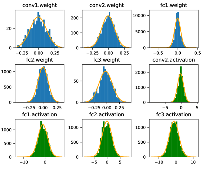
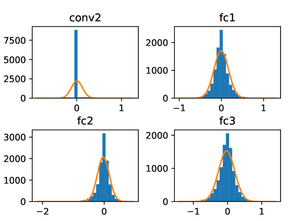
To further verify the distribution of weights and activations in neural networks, we take LeNet on CIFAR-10 as an example. Figure 1 shows the distributions of weights and activations on different layers of LeNet. It shows that the distribution is quite close to the fitted normal distribution model highlighted with orange color. We further have a bit error injected to a neuron in Conv2 of LeNet randomly. Then, we investigate the distribution of neuron errors in the following layers. Particularly, we take the first neuron in these layers as an example and fit the error distribution with a normal distribution model. The experiment result is shown in Figure 2. It can be observed that the neuron errors generally fit well with a normal distribution model centered at zero except that in Conv2 in which the input errors have not propagated comprehensively.
In addition, we assume the distribution of the weights and activations are independently and identically to simplify the modeling in the rest of this work. With the above assumptions, we can further derive the following lemmas.
Lemma 1
For a layer with neurons that follow independently identical normal distribution, the variance of sum of the neurons in the layer can be approximated with .
Lemma 2
For an output activation that is an accumulation of weighted input neurons , can be calculated with when the influence of activation function is ignored according to Proof 1. Note that stands for the total number of accumulated operations for a single neuron calculation. and refer to an neuron and a weight in th layer respectively.
Lemma 3
For an output activation error propagated from input activation errors, can be calculated with where represents the number of accumulation according to Proof 2.
Lemma 4
With the second and the third lemmas, we can conclude that . Hence, which indicates that keeps almost constant across different layers of an neural network.
Proof 1
Suppose and are two independent random variables following normal distribution, the variation of their product can be calculated with the product of their variation according to Equation 6. Since and can be considered as independent variables following normal distribution, we can conclude according to Equation 6 and Lemma 1.
| (6) |
Proof 2
An output activation error induced by neuron errors in previous layer can be formulated with Equation 7. Basically, an neuron error is essentially the accumulation of weighted input neuron errors. As mentioned, both neuron errors and weights can be characterized with normal distribution. In this case, the variation of an neuron error can also be calculated with according to Equation 6 and Lemma 1.
| (7) |
III-C Bit Flip Influence Modeling
To understand the influence of bit flip soft errors on neural network processing, we start to investigate the influence of bit flip on a single data. Take an activation quantized with int8 as an example, the quantized activation can be represented with Equation 8 where represents the dynamic range of activations in a layer of the neural network.
| (8) |
In this section, we mainly investigate the influence of quantization and the different fault injection methods on the resulting variations of activations. As mentioned before, we utilize RMSE as the metric to measure the activation variation caused by soft errors. Suppose the range of an activation is , a bit flip on most significant bit results in a change of . Similarly, a bit flip on the following bit leads a change of . In this case, the expected change of data i.e. quantized with int8 and int16 given a random bit flip can be represented with Equation 9 and Equation 10 respectively. When we double the , doubles. When the quantization data width doubles, shrinks by .
| (9) |
| (10) |
On top of the bit error influence of a single data, we scale the analysis to estimate the output data variation of a convolution operation induced by soft errors injected to either weights or activations. Suppose refers to the number of input channel, refers to the number of output channel, stands for the size of a feature map, refers to the size of a convolution kernel.
Disturbance in weights: Disturbance in a single weight affects output activations of an entire channel, i.e. activations. According to definition and Lemma 2 in Section III-B, the average variation of weights i.e. depends on the amount of input activations . . So the average computing variation of output activations can be calculated with Equation 11.
| (11) | ||||
Disturbance in activations: Suppose the average value of an activation in a layer is . Disturbance in a single activation will affect a window () of output activations in all the channels, i.e. activations. Suppose the feature map size is , then the average influence of the disturbance on an output activation can be calculated with Equation 12.
| (12) | ||||
Since the variation of activations and weights is generally constant given a specific model and data set according to the assumptions in Section III-B, RRMSE of a convolution layer that can be calculated with is consistent with RMSE accordingly.
III-D Relation between RRMSE and Classification Accuracy
Since the model accuracy of a typical classification task is based on statistics of a number of classification tasks and it is difficult to formulate with neural network computing directly, we utilize RRMSE defined in subsection III-A as an alternative metric to measure the influence of soft errors on model accuracy metric which is more closely related with neural network computing.
To begin, we start with a simple binary classification task and it includes only two output neurons in the last layer of the network. Then, the classification depends on larger output neuron. Suppose the two output neurons are and , and assume without loss of generality. When there are random errors injected to the neural network, the two output neurons follow normal distribution accordingly and they can be formulated with , according to Section III-B. In this case, the probability of wrong classification is essentially that of . The distribution of can be formulated with Equation 13, which is a shifted and scaled normal distribution model. Hence, the probability when can be calculated with Equation 14 where stands for cumulative distribution function of normal distribution.
| (13) |
| (14) | ||||
While in a typical binary classification task, Equation 14 can be converted to Equation 15 according to the definition of and in Section III-A.
| (15) | ||||
| (16) | ||||
| (17) |

For multi-class classification models, suppose there are classification types and the corresponding outputs of the classification model are denoted as . Assume the expected output is which is larger than any other output . Similar to the binary classification problem, a classification error happens when any of the outputs is larger than given Gaussian disturbance i.e. according to the definition of RRMSE. In this case, the model accuracy subjected to errors is the integration of the multiplication of the probability density function of and the cumulative distribution function of the rest outputs . It can be calculated with Equation 16.
Since the analytical model is usually difficult to calculate, we replace it with an empirical model as shown in Equation 17. It is essentially an sigmoid function variant and has two parameters i.e. and included. When there are no errors, the output of Equation 17 is the accuracy of a clean neural network model. When there are too many errors, the output of Equation 17 becomes which represents classification accuracy of random guessing. The empirical model can be determined given very few sampling data points of RRMSE and the corresponding classification accuracy.
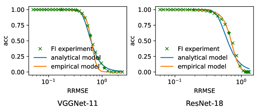
To verify the proposed models of correlation between RRMSE and neural network classification accuracy, we take VGGNet-11 and ResNet-18 on ImageNet as typical neural network examples to compare the analytical models and empirical models to the ground truth results. Particularly, we have two different evaluation approaches performed for the model comparison. In the first approach, we have a single true positive images from ImageNet utilized and repeat the execution for 10000 times on each error injection rate setup. It is denoted as single image analysis and it removes the influence of image variations from the analysis. In the second approach, we have 10000 different images randomly selected from ImageNet and evaluated for each error injection rate setup. It is denoted as multiple image analysis and it has the image variations incorporated in the analysis. For the soft error injection, we have 31 different bit error rate (BER) setups ranging from 1E-7 to 1E-4 conducted in the experiment. Ground truth of RRMSE and classification accuracy can be obtained from experiments directly. Analytical model can be determined given the RRMSE and while the empirical model can be determined with fitting on 4 data points evenly selected from ground truth data. The comparison is shown in Figure 3. It can be observed that the proposed analytical model is close to the ground truth data in the single image analysis setup but it has variation under multiple image analysis setup. This is expected as the proposed analytical model fails to characterize the influence of image variations. In contrast, empirical model fits much better on both single image analysis and multiple image analysis despite the lack of explainability. Nevertheless, it is clear that the model accuracy decreases monotonically with the increase of RRMSE, which allows us to characterize the influence of soft errors with RRMSE which can be obtained more conveniently compared to model accuracy.
III-E Error Influence Aggregation
In this section, we mainly explore how the influence of different errors aggregate on the same output neurons. Suppose represents RRMSE of an neural network output, it is the accumulation of independent random errors propagated from different layers. As mentioned, the influence of the random errors follows normal distribution model. The accumulation of these independent random errors can be formulated with Equation 18 where denotes the RRMSE induced by a neuron faults on layer . As the number of neurons in a neural network is extremely large, it remains timing consuming and inefficient to conduct neuron-wise fault analysis. To address the problem, we have Equation 18 further converted to layer-wise fault analysis where denotes RRMSE of neural network output caused by all the errors in layer and denotes the total number of neural network layers.
| (18) |
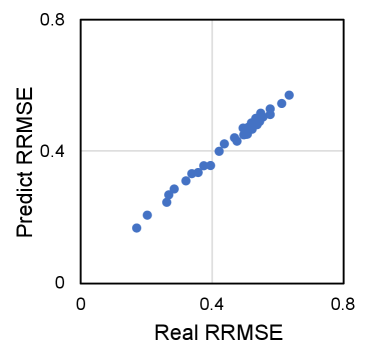
To verify the error aggregation model, we conduct layer-wise fault injection on VGGNet-11 and Resnet-18 quantized with int8 at different error injection rate . Then, we randomly select 32 different combination of layer-wise error injection configurations and compare the ground truth with that estimated with Equation 18. The comparison shown in Figure 4 reveals that the error aggregation model fits well with the simulation results and confirms the effectiveness of the model.
IV Modeling for Neural Network Resilience Analysis
With the above modeling of soft error influence on neural network accuracy, we can further utilize the models to analyze the influence of the major neural network design parameters on the resilience of neural networks subjected to soft errors, which can provide more general analysis compared to simulation based approaches. Specifically, we investigate influence of neural network layers, quantization, and number of classification types respectively on neural network resilience and they will be illustrated in detail in this section.
IV-A Influence of Number of Layers on NN Resilience
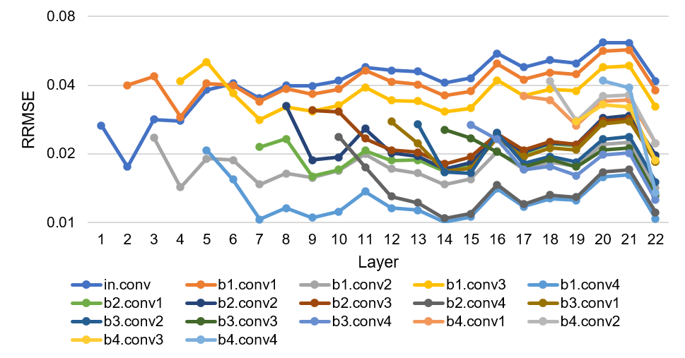
According to Lemma 4 in Section III-B, the output error metric of the th layer i.e. is almost constant across different layers of a neural network, which means that neural network depth does not have direct influence on neural network resilience. In order to verify this, we have random bit flip errors injected to neurons in different layers of VGGNet-11 and ResNet-18 respectively. The bit error rate is set to be 1E-6 in this experiment. Then, we evaluate RRMSE of the following layers of the neural networks over the corresponding golden reference output. RRMSE of the neural network layers is shown in Figure 5. It can be seen that RRMSE on different layers varies in a small range in general for each specific fault injection despite the layer locations of the error injection. Basically, it demonstrates that the influence of soft errors remains steady across the different layers and neural network depth will not affect the fault tolerance of the neural network model in general. It is true that small variations rather than constant as estimated in Lemma 4 can be found in RRMSE of different layers in Section III-B. This is mainly caused by the non-linear operations in neural networks which may filter out the computing errors and affect the error propagation.

IV-B Influence of Quantization on NN Resilience
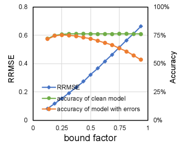
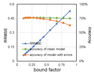
According to the analysis in Section III-D, we notice that quantization bound has straightforward influence on data variation induced by a single bit flip and affects RRMSE accordingly. Meanwhile, neural network models can choose different quantization bound with little accuracy loss in practice, so it can be expected that smaller quantization bound can improve the neural network model reliability subjected to soft errors without accuracy penalty. Figure 6 presents RRMSE of VGGNet-11 and ResNet-18 subjected to soft errors with various quantization bound while the bit error rate is set to be 1E-6. It reveals that RRMSE that is closely related with the neural network model accuracy as demonstrated in Section III-D increases almost linearly with the quantization bound experimented with all the different layers. On the other hand, we also observe that clean neural network classification accuracy remains steady in a wide range of quantization bound setups, which indicates that it is possible to improve the neural network reliability without accuracy penalty by choosing appropriate quantization bound.
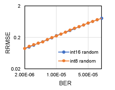
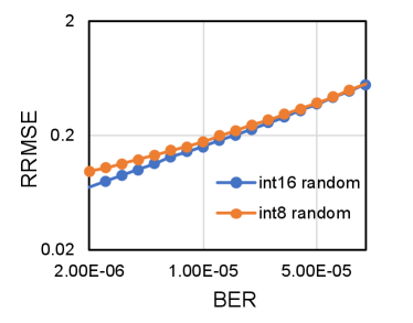
According to the comparison in Equation 9 and Equation 10, we notice that the average disturbance induced by a single bit error for neural network model quantized with int16 is smaller than that quantized with int8. On the other hand, the expected total number of bit errors for model quantized with int16 is twice larger than that quantized with int8 given the same bit error rate. According to Equation 18, of the same neural network model with more bit errors will be larger. Hence, of an neural network is equal to in theory given the same bit error rate. Similar to prior analysis, we take VGGNet-11 and ResNet-18 quantized with int8 and int16 as examples and conduct fault simulation to verify the model based analysis. The bit error rate is set to be 1E-6 and the quantization bound is set to be the same for both quantization data width. The experiment results shown in Figure 7 demonstrate that RRMSE of neural network models are generally steady despite the quantization data width, which is consistent with the model based analysis.
IV-C Influence of Classification Complexity on NN Resilience
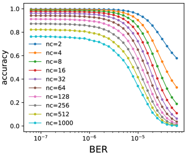
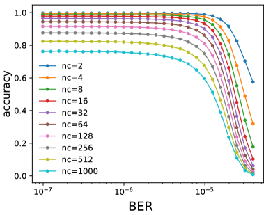
Intuitively, we notice that easier deep learning tasks are generally more resilient to errors, but it is usually difficult to define the complexity of a neural network processing task. Equation 16 provides a model to characterize the relation between the number of classification types and classification accuracy. When we take the number of classification types as a metric of neural network complexity, it provides a simple yet efficient angle to characterize the relation between neural network complexity and neural network resilience. The model in Equation 16 proves that neural networks with more classification types are more vulnerable subjected to the same number of errors. To verify this, we take VGGNet-11 and ResNet-18 on ImageNet as examples and then configure them for a set of classification tasks with different number of classification types i.e. ranging from 2 to 1000. Then, we explore the resulting accuracy of these classification tasks subjected to the same bit error setups. The experiment result is shown in Figure 8. It reveals that neural network models with less classification types generally have much higher accuracy and the accuracy drops slower with increasing bit error rate compared to that with more classification types.
V Modeling for Fault Simulation Acceleration
Fault simulation is a typical practice for neural network resilience analysis under hardware errors and several fault simulation tools [19] [4] [12] targeting at neural networks have been developed with different trade-offs between simulation accuracy and speed. Usually, a large number of errors need to be injected and a variety of fault configurations need to be explored to ensure steady simulation results, which can be rather time-consuming and expensive. Orthogonal to prior fault simulation approaches, we mainly investigate how the modeling proposed in this work can be utilized to accelerate the fault simulation with negligible simulation accuracy loss.
V-A Fault Simulation Acceleration Approaches
To begin, we will introduce three statistical model based approaches that can be utilized to accelerate general fault simulation. The basic idea is to leverage the proposed statistical models to predict the fault simulation results with only a fraction of simulation setups and reduce the number of fault simulation of all the possible fault configurations. The three acceleration approaches are listed as follows.
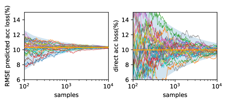
First, according to Equation 17, we can characterize the relation between RRMSE and model accuracy under various bit error rate setups with only five data points. Moreover, RRMSE of a model can be obtained with less input images and converges much faster than that of model accuracy. Particularly, we take VGGNet-11 on ImageNet as an example and investigate how the RRMSE and model accuracy of VGGNet-11 changes with different number of input image samples given the same bit error rate. The bit error rate is set to be 1E-6. The experiment result in Figure 9 confirms the advantage of using RRMSE in terms of convergence. With both the RRMSE and the correlation curve of RRMSE and model accuracy, we can obtain the correlation curve of bit error rate and model accuracy much faster compared to conventional fault simulation experiments.
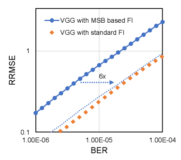
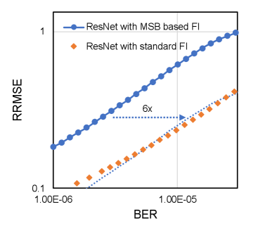
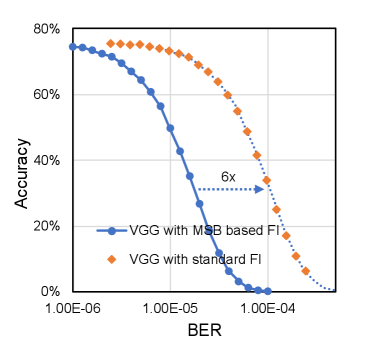
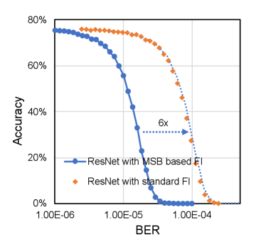
Second, with the analysis in Section III-C, we notice that the error injection on different bits contributes differently to the output RRMSE eventually but the contribution proportion can be calculated based on Equation 9 and Equation 10. Similarly, we can also obtain the expected data disturbance of bit error on MSB. Then, we can calculate based on with Equation 19 and 20, and replace the standard random bit error injection with most significant bit (MSB) based error injection without compromising the analysis accuracy. Take VGGNet-11 and ResNet-18 quantized with int16 as examples. Figure 10 shows the RRMSE obtained with both standard random bit error injection and MSB based error injection. It confirms that the resulting RRMSE obtained with standard error injection and MSB based error injection are linearly correlated as analyzed with the proposed statistical models. This approach can also be applied for straightforward model accuracy simulation. MSB based fault simulation and standard fault simulation for both VGGNet-11 and ResNet-18 is presented in Figure 11. It can be observed that the curves are quite similar and the difference is mainly induced by the scaled bit error rate. In summary, given the same bit error rate, MSB based error injection can be scaled for standard bit error injection with negligible accuracy penalty while it reduces the total number of injected bit errors substantially and enhances the fault simulation speed accordingly.
| (19) |
| (20) |
Third, according to the analysis in Section III-E, we notice that the influence of bit errors in different neurons and layers can be aggregated with Equation 18 when we utilize RRMSE as the accuracy metric. Based on this feature, we can analyze the influence of complex error configurations with a disaggregated approach. For instance, we can analyze the influence of random bit errors in each layer independently and then construct the influence of random bit errors on multiple neural network layers. We can also leverage the aggregation feature to scale RRMSE at lower bit error rate to RRMSE at higher bit error rate. In general, we can take advantage of this feature to obtain fault simulation of complex and large fault configurations with only a fraction of the fault configurations, which can greatly reduce the amount of fault simulation.
V-B Fault Simulation Acceleration Examples
To quantize the fault simulation speedup, we take two typical fault simulation tasks as examples.
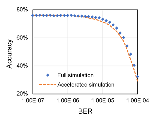
In the first task, we investigate how the model accuracy changes with the increase of bit error rate. We still utilize VGGNet-11 quantized with int16 on ImageNet as the benchmark model. Suppose we want to explore the model accuracy when the bit error rate changes from 1E-7 to 1E-4 and we take 32 evenly distributed bit error rate setups for the experiments. For each bit error rate setup, we take 10000 images from ImageNet to measure the model accuracy. With TensorFI fault injection framework [4], we need to conduct inference with bit error injection. The fault simulation task can be accelerated with the first and the second approaches. It needs only 4 fault simulation points of RRMSE and model accuracy with less bit error injection. The fault simulation time can be roughly reduced by . The results obtained with both a standard fault simulation and the accelerated fault simulation are shown in Figure 12. They are quite close to each other, which confirms the quality of the accelerated fault simulation.
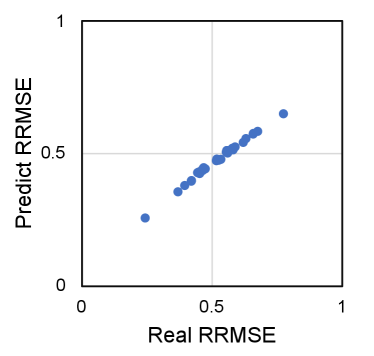
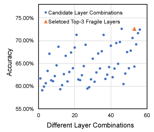
In the second task, we seek to find out the top-3 most fragile layers of a neural network model such that an selectively hardening approach can be applied to protect the neural network model with less protection overhead. We take VGGNet-11 quantized with int16 as a benchmark example and conduct fault injection at . There are 8 convolution layers in VGGNet-11. A standard fault simulation based method needs to evaluate all the different combinations. For each configuration, we need to perform inference on around 10000 images. Theoretically, we need to conduct inference with random bit error injection. In contrast, with the second and the third acceleration approaches, we only need to conduct 8 layer-wise MSB based error injection and perform inference on 1000 images for each error injection setup to obtain the neural network RRMSE. Then, we can obtain RRMSE of all the different layer combinations immediately according to Equation 18 in Section III. In this case, the fault simulation time can be reduced by . For neural networks with more layers, this method can achieve exponential acceleration. In addition, we also evaluate the selected top-3 fragile layers based on the accelerated fault simulation approach. Suppose the top-3 fragile layers are fault-free, we can obtain the model accuracy with standard fault simulation and compare with that of all the 56 different combinations. The experiment result is shown in Figure 13. It demonstrates that the selected top-3 layer are the most fragile layers of VGGNet-11, which is consistent with the results of standard fault simulation. In summary, the accelerated fault simulation not only reduces the execution time but also achieves high-quality results on this vulnerability analysis task.
VI Conclusion
In this work, we observe that soft errors propagate across a large number of neurons and accumulate. With the observation, we propose to characterize the disturbance induced by the soft errors with a normal distribution model according to central limit theorem and analyze the influence of soft errors on neural networks with a series of statistical models. The models are further applied to analyze the influence of convolutional neural network parameters on its resilience and verified with experiments comprehensively, which can guide the fault-tolerant neural network design. In addition, we find that the models can also be utilized to predict many fault simulation results precisely and avoid lengthy fault simulation in practice. Given two typical fault simulation tasks, the model-accelerated fault simulation can be more than two orders of magnitude faster on average with negligible accuracy loss compared to standard fault simulation.
References
- [1] Muhammad Atta Othman Ahmed. Trained Neural Networks Ensembles Weight Connections Analysis. Advances in Intelligent Systems and Computing, 723(January):242–251, 2018.
- [2] Subho S. Banerjee, James Cyriac, Saurabh Jha, Zbigniew T. Kalbarczyk, and Ravishankar K. Iyer. Towards a Bayesian Approach for Assessing Fault Tolerance of Deep Neural Networks. Proceedings - 49th Annual IEEE/IFIP International Conference on Dependable Systems and Networks - Supplemental Volume, DSN-S 2019, pages 25–26, 2019.
- [3] Zitao Chen, Guanpeng Li, Karthik Pattabiraman, and Nathan DeBardeleben. Binfi: An efficient fault injector for safety-critical machine learning systems. In Proceedings of the International Conference for High Performance Computing, Networking, Storage and Analysis, SC ’19, New York, NY, USA, 2019. Association for Computing Machinery.
- [4] Zitao Chen, Niranjhana Narayanan, Bo Fang, Guanpeng Li, Karthik Pattabiraman, and Nathan DeBardeleben. Tensorfi: A flexible fault injection framework for tensorflow applications. Proceedings - International Symposium on Software Reliability Engineering, ISSRE, 2020-Octob:426–435, 2020.
- [5] Anand Dixit and Alan Wood. The impact of new technology on soft error rates. In 2011 International Reliability Physics Symposium, pages 5B–4. IEEE, 2011.
- [6] Fernando Fernandes dos Santos, Caio Lunardi, Daniel Oliveira, Fabiano Libano, and Paolo Rech. Reliability evaluation of mixed-precision architectures. In 2019 IEEE International Symposium on High Performance Computer Architecture (HPCA), pages 238–249. IEEE, 2019.
- [7] Gianni Franchi, Andrei Bursuc, Emanuel Aldea, Séverine Dubuisson, and Isabelle Bloch. TRADI: Tracking Deep Neural Network Weight Distributions. Lecture Notes in Computer Science (including subseries Lecture Notes in Artificial Intelligence and Lecture Notes in Bioinformatics), 12362 LNCS:105–121, 2020.
- [8] Giulio Gambardella, Johannes Kappauf, Michaela Blott, Christoph Doehring, Martin Kumm, Peter Zipf, and Kees Vissers. Efficient error-tolerant quantized neural network accelerators. In 2019 IEEE International Symposium on Defect and Fault Tolerance in VLSI and Nanotechnology Systems (DFT), pages 1–6. IEEE, 2019.
- [9] Zhen Gao, Han Zhang, Yi Yao, Jiajun Xiao, Shulin Zeng, Guangjun Ge, Yu Wang, Anees Ullah, and Pedro Reviriego. Soft error tolerant convolutional neural networks on fpgas with ensemble learning. IEEE Transactions on Very Large Scale Integration (VLSI) Systems, 30(3):291–302, 2022.
- [10] Siva Kumar Sastry Hari, Timothy Tsai, Mark Stephenson, Stephen W. Keckler, and Joel Emer. SASSIFI: An architecture-level fault injection tool for GPU application resilience evaluation. ISPASS 2017 - IEEE International Symposium on Performance Analysis of Systems and Software, 1(1):249–258, 2017.
- [11] Daniel A Hashimoto, Guy Rosman, Daniela Rus, and Ozanan R Meireles. Artificial intelligence in surgery: promises and perils. Annals of surgery, 268(1):70, 2018.
- [12] Yi He, Prasanna Balaprakash, and Yanjing Li. Fidelity: Efficient resilience analysis framework for deep learning accelerators. Proceedings of the Annual International Symposium on Microarchitecture, MICRO, 2020-Octob:270–281, 2020.
- [13] Nargiz Humbatova, Gunel Jahangirova, Gabriele Bavota, Vincenzo Riccio, Andrea Stocco, and Paolo Tonella. Taxonomy of real faults in deep learning systems. In Proceedings of the ACM/IEEE 42nd International Conference on Software Engineering, pages 1110–1121, 2020.
- [14] Guanpeng Li, Siva Kumar Sastry Hari, Michael B. Sullivan, Timothy Tsai, Karthik Pattabiraman, Joel S. Emer, and Stephen W. Keckler. Understanding error propagation in deep learning neural network (DNN) accelerators and applications. In Bernd Mohr and Padma Raghavan, editors, Proceedings of the International Conference for High Performance Computing, Networking, Storage and Analysis, SC 2017, Denver, CO, USA, November 12 - 17, 2017, pages 8:1–8:12. ACM, 2017.
- [15] Wenshuo Li, Xuefei Ning, Guangjun Ge, Xiaoming Chen, Yu Wang, and Huazhong Yang. Ftt-nas: Discovering fault-tolerant neural architecture. In 2020 25th Asia and South Pacific Design Automation Conference (ASP-DAC), pages 211–216. IEEE, 2020.
- [16] Fabiano Libano, Brittany Wilson, J Anderson, Michael J Wirthlin, Carlo Cazzaniga, Christopher Frost, and Paolo Rech. Selective hardening for neural networks in fpgas. IEEE Transactions on Nuclear Science, 66(1):216–222, 2018.
- [17] Cheng Liu, Cheng Chu, Dawen Xu, Ying Wang, Qianlong Wang, Huawei Li, Xiaowei Li, and Kwang-Ting Cheng. Hyca: A hybrid computing architecture for fault tolerant deep learning. IEEE Transactions on Computer-Aided Design of Integrated Circuits and Systems, 2021.
- [18] Cheng Liu, Zhen Gao, Siting Liu, Xuefei Ning, Huawei Li, and Xiaowei Li. Special session: Fault-tolerant deep learning: A hierarchical perspective. In 2022 IEEE 40th VLSI Test Symposium (VTS), pages 1–12. IEEE, 2022.
- [19] Abdulrahman Mahmoud, Neeraj Aggarwal, Alex Nobbe, Jose Rodrigo Sanchez Vicarte, Sarita V. Adve, Christopher W. Fletcher, Iuri Frosio, and Siva Kumar Sastry Hari. PyTorchFI: A Runtime Perturbation Tool for DNNs. Proceedings - 50th Annual IEEE/IFIP International Conference on Dependable Systems and Networks, DSN-W 2020, pages 25–31, 2020.
- [20] Sparsh Mittal. A survey on modeling and improving reliability of dnn algorithms and accelerators. Journal of Systems Architecture, 104:101689, 2020.
- [21] Khan Muhammad, Amin Ullah, Jaime Lloret, Javier Del Ser, and Victor Hugo C de Albuquerque. Deep learning for safe autonomous driving: Current challenges and future directions. IEEE Transactions on Intelligent Transportation Systems, 22(7):4316–4336, 2020.
- [22] Xuefei Ning, Guangjun Ge, Wenshuo Li, Zhenhua Zhu, Yin Zheng, Xiaoming Chen, Zhen Gao, Yu Wang, and Huazhong Yang. Ftt-nas: Discovering fault-tolerant convolutional neural architecture. ACM Transactions on Design Automation of Electronic Systems (TODAES), 26(6):1–24, 2021.
- [23] Shane O’Sullivan, Nathalie Nevejans, Colin Allen, Andrew Blyth, Simon Leonard, Ugo Pagallo, Katharina Holzinger, Andreas Holzinger, Mohammed Imran Sajid, and Hutan Ashrafian. Legal, regulatory, and ethical frameworks for development of standards in artificial intelligence (ai) and autonomous robotic surgery. The international journal of medical robotics and computer assisted surgery, 15(1):e1968, 2019.
- [24] Elbruz Ozen and Alex Orailoglu. SNR: Squeezing Numerical Range Defuses Bit Error Vulnerability Surface in Deep Neural Networks. ACM Trans. Embed. Comput. Syst., 20(5s), 2021.
- [25] Pramesh Pandey, Prabal Basu, Koushik Chakraborty, and Sanghamitra Roy. Greentpu: Improving timing error resilience of a near-threshold tensor processing unit. In 2019 56th ACM/IEEE Design Automation Conference (DAC), pages 1–6. IEEE, 2019.
- [26] Samira Pouyanfar, Saad Sadiq, Yilin Yan, Haiman Tian, Yudong Tao, Maria Presa Reyes, Mei-Ling Shyu, Shu-Ching Chen, and Sundaraja S Iyengar. A survey on deep learning: Algorithms, techniques, and applications. ACM Computing Surveys (CSUR), 51(5):1–36, 2018.
- [27] Brandon Reagen, Udit Gupta, Lillian Pentecost, Paul Whatmough, Sae Kyu Lee, Niamh Mulholland, David Brooks, and Gu Yeon Wei. Ares: A framework for quantifying the resilience of deep neural networks. In Proceedings - Design Automation Conference, volume Part F1377, 2018.
- [28] Brandon Reagen, Paul Whatmough, Robert Adolf, Saketh Rama, Hyunkwang Lee, Sae Kyu Lee, José Miguel Hernández-Lobato, Gu-Yeon Wei, and David Brooks. Minerva: Enabling low-power, highly-accurate deep neural network accelerators. In 2016 ACM/IEEE 43rd Annual International Symposium on Computer Architecture (ISCA), pages 267–278. IEEE, 2016.
- [29] Albert Reuther, Peter Michaleas, Michael Jones, Vijay Gadepally, Siddharth Samsi, and Jeremy Kepner. Survey and benchmarking of machine learning accelerators. In 2019 IEEE high performance extreme computing conference (HPEC), pages 1–9. IEEE, 2019.
- [30] Albert Reuther, Peter Michaleas, Michael Jones, Vijay Gadepally, Siddharth Samsi, and Jeremy Kepner. Ai accelerator survey and trends. In 2021 IEEE High Performance Extreme Computing Conference (HPEC), pages 1–9. IEEE, 2021.
- [31] Muhammad Shafique, Mahum Naseer, Theocharis Theocharides, Christos Kyrkou, Onur Mutlu, Lois Orosa, and Jungwook Choi. Robust machine learning systems: Challenges, current trends, perspectives, and the road ahead. IEEE Design & Test, 37(2):30–57, 2020.
- [32] Cesar Torres-Huitzil and Bernard Girau. Fault and error tolerance in neural networks: A review. IEEE Access, 5:17322–17341, 2017.
- [33] Dawen Xu, Meng He, Cheng Liu, Ying Wang, Long Cheng, Huawei Li, Xiaowei Li, and Kwang-Ting Cheng. R2f: A remote retraining framework for aiot processors with computing errors. IEEE Transactions on Very Large Scale Integration (VLSI) Systems, 29(11):1955–1966, 2021.
- [34] Dawen Xu, Ziyang Zhu, Cheng Liu, Ying Wang, Huawei Li, Lei Zhang, and Kwang-Ting Cheng. Persistent fault analysis of neural networks on fpga-based acceleration system. In 2020 IEEE 31st International Conference on Application-specific Systems, Architectures and Processors (ASAP), pages 85–92. IEEE, 2020.
- [35] Dawen Xu, Ziyang Zhu, Cheng Liu, Ying Wang, Shuang Zhao, Lei Zhang, Huaguo Liang, Huawei Li, and Kwang-Ting Cheng. Reliability evaluation and analysis of fpga-based neural network acceleration system. IEEE Transactions on Very Large Scale Integration (VLSI) Systems, 29(3):472–484, 2021.
- [36] Xinghua Xue, Haitong Huang, Cheng Liu, Ying Wang, Tao Luo, and Lei Zhang. Winograd convolution: A perspective from fault tolerance. arXiv preprint arXiv:2202.08675, 2022.
- [37] Jeff Jun Zhang, Tianyu Gu, Kanad Basu, and Siddharth Garg. Analyzing and mitigating the impact of permanent faults on a systolic array based neural network accelerator. In 2018 IEEE 36th VLSI Test Symposium (VTS), pages 1–6. IEEE, 2018.
- [38] Yang Zheng, Zhenye Feng, Zheng Hu, and Ke Pei. Mindfi: A fault injection tool for reliability assessment of mindspore applicacions. In 2021 IEEE International Symposium on Software Reliability Engineering Workshops (ISSREW), pages 235–238, 2021.