22institutetext: Queen Mary University of London, London, United Kingdom,
33institutetext: Memorial University of Newfoundland, NL, Canada,
44institutetext: Western University, London, ON, Canada
Statistical network isomorphism
Abstract
Graph isomorphism is a problem for which there is no known polynomial-time solution. Nevertheless, assessing (dis)similarity between two or more networks is a key task in many areas, such as image recognition, biology, chemistry, computer and social networks. Moreover, questions of similarity are typically more general and their answers more widely applicable than the more restrictive isomorphism question. In this article, we offer a statistical answer to the following questions: a) “Are networks and similar?”, b) “How different are the networks and ?” and c) “Is more similar to or ?”. Our comparisons begin with the transformation of each graph into an all-pairs distance matrix. Our node-node distance, Jaccard distance, has been shown to offer a good reflection of the graph’s connectivity structure. We then model these distances as probability distributions. Finally, we use well-established statistical tools to gauge the (dis)similarities in terms of probability distribution (dis)similarity. This comparison procedure aims to detect (dis)similarities in connectivity structure, not in easily observable graph characteristics, such as degrees, edge counts or density. We validate our hypothesis that graphs can be meaningfully summarized and compared via their node-node distance distributions, using several synthetic and real-world graphs. Empirical results demonstrate its validity and the accuracy of our comparison technique.
Note on terminology: For the sake of compactness, the work in this article focuses exclusively on simple graphs. We only consider unweighted, undirected graphs with no self-loops or multiple edges. Throughout this article, the terms graph and network are used interchangeably. Similarly, the terms vertex and node and the terms edge, arc, link and connection are used as synonyms.
1 Introduction
Graph isomorphism is a problem for which there is no known polynomial-time solution. Nevertheless, assessing network (dis)similarity is a key task in many areas, such as image recognition, biology, chemistry, computer and social networks. In this article, we offer a statistical answer to the following questions: a) “Are networks and similar?”, b) “How different are the networks and ?” and c) “Is more similar to or ?”. It is important to note here that these questions are more general and their answers more widely applicable than the more restrictive isomorphism question.
We obtain these answers by first converting networks (graphs) into an all pairs distances matrix. To achieve this transformation, we use Jaccard distance instead of the typically used shortest-path or the also common random walk-based distances (e.g., commute, resistance,…). Previous work has highlighted the shortcomings of shortest-path [1] and random walk-based distances [15, 16, 21]. The advantages of Jaccard distance, especially its relation to connectivity structure, have also been demonstrated [3, 19, 18].
Our comparison technique is focused on comparing each network’s connectivity structure, not on easily observable graph characteristics such as vertex or edge counts. We argue that changes in connectivity may be indicative of critical network event occurrences, which makes structural conectivity-based (dis)similarity worthy of investigation. For example, the presence of denser subgraphs may indicate a loss of connection to the broader network and the appearance of bottlenecks, in a physical or computer network. They can also be an indicator of malicious activity, especially of the multi-party coordinated variety [23, 27, 26].
As described later in this article, Jaccard distance also has a probabilistic interpretation. On the basis of this interpretation, we then compare networks as probability distributions of distances, using well-established statistical techniques. Our comparisons are not restricted to a few key statistical or graph characteristics, such as mean distance, mean degree or diameter. Instead, our conversion to a distance matrix and interpretation of these distances as a probability distribution captures each graph’s entire connectivity structure.
2 Previous work
The comparison of static graphs and the study of temporal graphs are overlapping topics. Indeed, the study of temporal graphs naturally includes comparisons of snapshots of time-evolving graphs. In the past, several authors have highlighted the need to study graph similarity and their evolution over time. These authors have illustrated their claims using various areas of application, areas as varied as image recognition [2], network robustness and resilience [13], mobile telephony [24, 13, 6] and public transportation [17]. Notably, graph comparisons and temporal graphs remain current topics of inquiry [11, 5, 25].
A full review of the graph similarity and temporal graphs literature is beyond the scope of this short article. However, we wish to highlight the fact that this article is built upon the foundations of Schieber et al. [22] and the very recent work of Wang et al. [25]. These authors have modeled graphs as probability distributions.
3 Methods
We model graphs as probability distributions of vertex-vertex distances. We too posit that graphs can be meaningfully summarized and compared on the basis of their node-node distances. Just as others before us, we begin by obtaining the distances between all vertex pairs. However, unlike in previous work, we use Jaccard distances [12, 3, 19, 18]. The main difference between earlier work and ours lies in the choice of node-node distance.
Schieber et al. [22] use shortest path distance. However, previous work has highlighted its shortcomings. For example, Akara-pipattana et al. [1] stated the following: “While intuitive and visual, this notion of distance is limited in that it does not fully capture the ease or difficulty of reaching point j from point i by navigating the graph edges. It does not say whether there is only one path of minimal length or many such paths, whether these paths can be straightforwardly located, or whether alternative paths are considerably or only slightly longer”. In the past, Chebotarev and Shamis [4] as well as Fouss et al. [7] have also highlighted the unsuitability of shortest-path distance as a similarity measure between vertices. We have also echoed these assertions in recent publications and have demonstrated the superiority of the Jaccard distance as a reflection of graph structure [19, 18].
In their very recent work, Wang et al. [25] use a combination of embedding and Euclidean distance. While they report interesting results, this two-step process appears cumbersome and ill-suited to larger graphs, at first glance. Arguably, embedding graphs into vector space carries a non-trivial computational cost. In this specific case, the authors use the DeepWalk algorithm [20] to obtain their embedding. While the creators of DeepWalk claim their technique is scalable and parallelizable, it simulates random walks across the network. In contrast, Jaccard distance only relies on simple vertex-pair level arithmetic computations, instead of multiple layers of neighborhoods, and has been shown to offer an accurate reflection of graph structure [19, 18]. Its computation can also be easily performed incrementally or in parallel. In addition, several authors have highlighted the breakdown of the random-walk based commute (resistance) distance in the case of larger graphs [15, 16, 21].
We would also like to draw attention to the fact some authors restrict their comparisons to graphs with equal numbers of nodes [8]. Yet, others are interested in the more general case of comparisons between graph with unequal numbers of nodes [14]. Because we compare connectivity through cumulative distributions, the number of nodes in each graph is not relevant. Our technique applies equally to either case.
3.1 Vertex-vertex Jaccard distance
The Jaccard distance separating two vertices and is defined as
Here, represents the set of all vertices with which vertex shares an edge. The ratio is the well known Jaccard similarity. The Jaccard distance () is its complement.
3.1.1 Probabilistic interpretation of the Jaccard distance
The Jaccard similarity () between two nodes and can be interpreted probabilistically. Consider all nodes of a network, excluding and , and select at random a node . The Jaccard similarity is then an estimate of the (conditional) probability that both and are connected to , given that at least one of and is connected to . Mathematically, we express as,
where indicates the existence of an edge between nodes and .
The Jaccard distance () is its complement. It can be interpreted as one of these two cases:
-
a)
the (conditional) probability that is connected to , but is not,
(exclusive) or
-
b)
the (conditional) probability that is connected to , but is not.
Mathematically, we express it as
3.1.2 From graph to empirical probability distribution
Once all distances have been obtained, we examine their statistical distribution. On the basis of the probabilistic interpretation of the just described, we treat these quantities as random variables. This model allows us to study and compare graphs as empirical probability distributions of node-node distances.
Figure 1 illustrates the interpretation of a graph as a probability distribution. The image on the left shows the distribution of node-node distances for an Erdős-Rényi (ER) graph with an edge probability of . The image on the right is of the distribution of distances between nodes of a stochastic block model graph (SBM) of varying cluster sizes and in/out edge probabilities of .
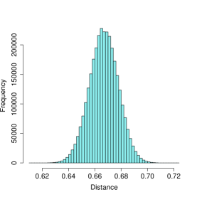
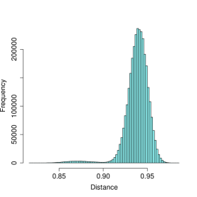
The structural differences between these two graphs is immediately obvious. The ER graph’s distances are symmetrically distributed about their mean, in a Gaussian-like pattern. In stark contrast, the SBM graph’s distances are left-skewed and bi-modal. The left mode reflects distances between nodes in the same blocks, whereas the right mode reflects distances between nodes not in the same blocks. Naturally, this pattern does not occur under the ER model.
3.2 Dissimilarity of probability distributions
We compare the networks of interest via the empirical probability distributions of the Jaccard distances between their nodes. To perform these comparisons, we use the Kolmogorov-Smirnov (K-S) distance and the Wasserstein distance of order . These distances are defined as follows: In a comparison between two networks, let be the empirical cumulative distribution function (CDF) of Jaccard distances for the first network, and the empirical CDF of Jaccard distances for the second network ( denotes the inverse CDF). The Kolmogorov-Smirnov (K-S) distance to compare and is defined as
Meanwhile, the Wasserstein distance of order between and is defined as
(In our experiments, we set the parameter .)
The K-S distance metric is also a test statistic. In this specific case, it is a test statistic for the two-sample K-S test. The hypotheses of this test are listed below.
-
•
Null hypothesis () : the two samples are drawn from the same distribution
-
•
Alternative hypothesis () : the two samples are drawn from different distributions
The -values of the K-S test provide an interpretation and validation of the test statistic (distance). They give us the probability of obtaining a distance metric of the same or greater magnitude, under the (null) hypothesis that both samples were drawn from the same distribution. Small -values provide evidence that the maximum vertical distance between the empirical CDFs of two compared graphs is statistically significantly different from zero. These -values are obtained from the Kolmogorov distribution.
While the K-S distance is always contained in the interval , the Wasserstein distance is not. To make comparisons more meaningful and easier to interpret, we transform the latter, so that it also lies on the same interval. After obtaining the quantity , we perform the following transformation,
In our comparisons, we use the quantity .
4 Numerical results
We validate our hypothesis that graphs can be meaningfully summarized and compared via their node-node distance distributions, using several synthetic and real-world graphs. Their key characteristics are reported in Table 1. The columns correspond to
-
•
: number of vertices,
-
•
: number of edges,
-
•
: density,
-
•
: minimum degree,
-
•
: mean degree,
-
•
: maximumm degree and
-
•
: number of connected components.
| Synthetic | ER.333 | 2,500 | 1,039,694 | 0.33 | 753 | 831.76 | 929 | 1 |
| ER.35 | 2,500 | 1,092,408 | 0.35 | 794 | 873.93 | 944 | 1 | |
| ER.5 | 2,500 | 1,562,067 | 0.50 | 1,157 | 1,249.65 | 1,344 | 1 | |
| ER.3332cc | 2,500 | 887,948 | 0.28 | 45 | 710.36 | 843 | 2 | |
| ER.333N1K | 1,000 | 166,417 | 0.33 | 289 | 332.83 | 381 | 1 | |
| SBM0701 | 2,495 | 348,674 | 0.11 | 230 | 279.50 | 334 | 1 | |
| SBM0901 | 2,495 | 360,867 | 0.12 | 235 | 289.27 | 346 | 1 | |
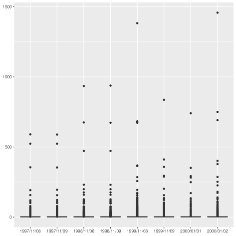
| Real-world | 1997/11/08 | 3,015 | 5,156 | 0.00 | 1 | 3.42 | 590 | 1 |
| 1997/11/09 | 3,011 | 5,150 | 0.00 | 1 | 3.42 | 589 | 1 | |
| 1998/11/08 | 4,296 | 7,815 | 0.00 | 1 | 3.64 | 935 | 1 | |
| 1998/11/09 | 4,301 | 7,838 | 0.00 | 1 | 3.64 | 938 | 1 | |
| 1999/11/08 | 6,127 | 12,046 | 0.00 | 1 | 3.93 | 1,383 | 1 | |
| 1999/11/09 | 3,962 | 7,931 | 0.00 | 1 | 4.00 | 837 | 1 | |
| 2000/01/01 | 3,570 | 7,033 | 0.00 | 1 | 3.94 | 740 | 1 | |
| 2000/01/02 | 6,474 | 12,572 | 0.00 | 1 | 3.88 | 1,458 | 1 |
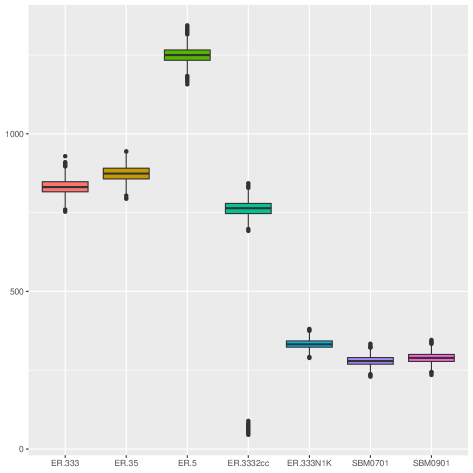
The generative models used to create the synthetic graphs are listed below. These graphs were generated using the NetworkX library [9].
-
•
ER.333: ER with
-
•
ER.35: ER with
-
•
ER.5: ER with
-
•
ER.3332cc: ER also with , but with two connected components ()
-
•
ER.333N1K: ER also with , but with only
-
•
SBM0701: stochastic block model, with clusters in range of and
-
•
SBM0901: stochastic block model, with clusters in range of and
Meanwhile, the real-world graphs were obtained from the Harvard Dataverse repository [10]. These data sets are from the University of Oregon’s “Route Views Project”. Each graph contains a daily snapshot of a set of internet “autonomous systems” and their connections.
| ER.333 | ER.35 | ER.5 | ER.3332cc | ER.333N1K | SBM0701 | SBM0901 | |
|---|---|---|---|---|---|---|---|
| ER.333 | NA | 0.01 | 0.13 | 0.07 | 0.01 | 0.13 | 0.13 |
| ER.35 | NA | NA | 0.11 | 0.07 | 0.01 | 0.14 | 0.14 |
| ER.5 | NA | NA | NA | 0.16 | 0.13 | 0.24 | 0.24 |
| ER.3332cc | NA | NA | NA | NA | 0.06 | 0.12 | 0.12 |
| ER.333N1K | NA | NA | NA | NA | NA | 0.13 | 0.13 |
| SBM0701 | NA | NA | NA | NA | NA | NA | 0.00 |
| SBM0901 | NA | NA | NA | NA | NA | NA | NA |
| 1997/11/08 | 1997/11/09 | 1998/11/08 | 1998/11/09 | 1999/11/08 | 1999/11/09 | 2000/01/01 | 2000/01/02 | |
|---|---|---|---|---|---|---|---|---|
| 1997/11/08 | NA | 0.00 | 0.03 | 0.03 | 0.04 | 0.04 | 0.04 | 0.04 |
| 1997/11/09 | NA | NA | 0.03 | 0.03 | 0.04 | 0.04 | 0.04 | 0.04 |
| 1998/11/08 | NA | NA | NA | 0.00 | 0.02 | 0.03 | 0.03 | 0.02 |
| 1998/11/09 | NA | NA | NA | NA | 0.02 | 0.03 | 0.03 | 0.02 |
| 1999/11/08 | NA | NA | NA | NA | NA | 0.02 | 0.02 | 0.01 |
| 1999/11/09 | NA | NA | NA | NA | NA | NA | 0.01 | 0.02 |
| 2000/01/01 | NA | NA | NA | NA | NA | NA | NA | 0.02 |
| 2000/01/02 | NA | NA | NA | NA | NA | NA | NA | NA |
| ER.333 | ER.35 | ER.5 | ER.3332cc | ER.333N1K | SBM0701 | SBM0901 | |
| ER.333 | NA | 0.43 | 1.00 | 0.15 | 0.11 | 1.00 | 1.00 |
| (0.00) | (0.00) | (0.00) | (0.00) | (0.00) | (0.00) | ||
| ER.35 | NA | NA | 1.00 | 0.46 | 0.38 | 1.00 | 1.00 |
| (0.00) | (0.00) | (0.00) | (0.00) | (0.00) | |||
| ER.5 | NA | NA | NA | 1.00 | 1.00 | 1.00 | 1.00 |
| (0.00) | (0.00) | (0.00) | (0.00) | ||||
| ER.3332cc | NA | NA | NA | NA | 0.15 | 0.85 | 0.85 |
| (0.00) | (0.00) | (0.00) | |||||
| ER.333N1K | NA | NA | NA | NA | NA | 1.00 | 1.00 |
| (0.00) | (0.00) | ||||||
| SBM0701 | NA | NA | NA | NA | NA | NA | 0.07 |
| (0.00) | |||||||
| SBM0901 | NA | NA | NA | NA | NA | NA | NA |
| 1997/11/08 | 1997/11/09 | 1998/11/08 | 1998/11/09 | 1999/11/08 | 1999/11/09 | 2000/01/01 | 2000/01/02 | |
| 1997/11/08 | NA | 0.00 | 0.01 | 0.01 | 0.01 | 0.02 | 0.02 | 0.01 |
| (0.98) | (0.00) | (0.00) | (0.00) | (0.00) | (0.00) | (0.00) | ||
| 1997/11/09 | NA | NA | 0.01 | 0.01 | 0.01 | 0.02 | 0.02 | 0.01 |
| (0.00) | (0.00) | (0.00) | (0.00) | (0.00) | (0.00) | |||
| 1998/11/08 | NA | NA | NA | 0.00 | 0.01 | 0.01 | 0.02 | 0.01 |
| (0.87) | (0.00) | (0.00) | (0.00) | (0.00) | ||||
| 1998/11/09 | NA | NA | NA | NA | 0.01 | 0.01 | 0.02 | 0.01 |
| (0.00) | (0.00) | (0.00) | (0.00) | |||||
| 1999/11/08 | NA | NA | NA | NA | NA | 0.01 | 0.02 | 0.00 |
| (0.00) | (0.00) | (0.00) | ||||||
| 1999/11/09 | NA | NA | NA | NA | NA | NA | 0.00 | 0.01 |
| (0.00) | (0.00) | |||||||
| 2000/01/01 | NA | NA | NA | NA | NA | NA | NA | 0.02 |
| (0.00) | ||||||||
| 2000/01/02 | NA | NA | NA | NA | NA | NA | NA | NA |
Our results show that our technique based on a transformation from graph to probability distribution and distance measurements with either the Wasserstein and K-S distances between node-node distributions are valid measures of network (dis)similarity. Indeed, these metrics accurately identify network structure changes, even in arguably difficult cases. For example, both metrics accurately detect the disconnection into two connected components of the ER graph with probability (ER.333 vs. ER.3332cc).
Our results also confirm that our procedure correctly identifies the structural stability of the internet networks. In fact, our procedure is robust to degree outliers that are very common in real-world networks. Arguably, while the number of nodes and edges of internet networks do vary, the graph’s connectivity structure remains constant. This robustness is reflected in the small distance between the distributions.
Even so, here, we must also acknowledge the limitations of our method. While our network comparison technique is indeed robust to degree outliers, it does correctly detect changes in the number of edges and vertices and classify these networks as significantly different. However, the magnitude of their difference is very small, which is why we highlight robustness. For example, in the comparison between internet networks, our technique correctly identifies the difference between graphs 2000/01/01 and 2000/01/02 as statistically significant (). As mentioned earlier, the magnitude of the difference is very low (), in spite of a very significant difference in the number of edges and vertices. This low distance variation in response to large node and edge count variations in the distances between CDFs may be considered a limitation. For this reason, we caution against interpreting absolute magnitudes of distances without testing for significance.
Nevertheless, it must be noted that these graphs appear to be rather similar, from a structural point of view. Indeed, both networks, have equal density and a very similar degree distribution. We posit that the magnitude of the difference remains small, although statistically significant, due to the structural similarity of these networks. Meanwhile, in the comparison between the ER graphs with 1,000 and 2,500 nodes (ER.333 vs. ER.333N1K), our technique did correctly identify a variation in network structure and a greater dissimilarity (distance) between these graphs. While these two graphs share the same edge probability parameter, their degree distributions differ significantly.
Finally, we must also offer a comparison of our technique to arguably simpler to obtain network characteristics, namely density and degree distribution. While density does indeed offer valuable information about a graph’s structure, a comparison of densities is not sufficient to detect a change in structure. For example, the graphs ER.333 and ER.333N1K have identical densities, yet have significantly different degree distributions. Also, a graph’s density does not offer any information regarding local connection patterns, such as community structure for example.
Degree distribution also offers very valuable information about a network. Again, a comparison of degree distributions only offers a partial assessment of (dis)similarity. For example, the ER.333 and ER.333N1K graphs have significantly different degree distributions, yet have very similar connectivity patterns. Our two stochastic block model graphs (SBM0701 and SBM0901) have degree distributions that are very similar to the ER.333N1K, yet their connectivity (community) structure is totally different.
5 Conclusion
In this article, we present a statistical graph comparison technique which is based on node-node distances. Our results show that our technique accurately detects differences in graph structure. Future work will focus on statistical comparisons via sampling, which should offer greater scalability for our comparison technique. Naturally, we will also conduct further tests, using different scenarios.
References
- [1] Akara-pipattana, P., Chotibut, T., Evnin, O.: Resistance distance distribution in large sparse random graphs. arXiv e-prints arXiv:2107.12561 (2021)
- [2] Bunke, H.: Graph matching: Theoretical foundations, algorithms, and applications. Proc Vision Interface 2000 21 (01 2000)
- [3] Camby, E., Caporossi, G.: The extended Jaccard distance in complex networks. Les Cahiers du GERAD G-2017-77 (09 2017)
- [4] Chebotarev, P., Shamis, E.: The Matrix-Forest Theorem and Measuring Relations in Small Social Groups. arXiv Mathematics e-prints math/0602070 (2006)
- [5] Coupette, C., Vreeken, J.: Graph similarity description: How are these graphs similar? In: Proceedings of the 27th ACM SIGKDD Conference on Knowledge Discovery and Data Mining. pp. 185–195. KDD ’21, Association for Computing Machinery, New York, NY, USA (2021), https://doi.org/10.1145/3447548.3467257
- [6] Du, Z., Yang, Y., Gao, C., Huang, L., Huang, Q., Bai, Y.: The temporal network of mobile phone users in Changchun Municipality, Northeast China. Scientific Data 5, 180228 (10 2018)
- [7] Fouss, F., Francoisse, K., Yen, L., Pirotte, A., Saerens, M.: An experimental investigation of kernels on graphs for collaborative recommendation and semisupervised classification. Neural Networks 31, 53–72 (2012), https://www.sciencedirect.com/science/article/pii/S0893608012000822
- [8] Grohe, M., Rattan, G., Woeginger, G.: Graph Similarity and Approximate Isomorphism. arXiv e-prints arXiv:1802.08509 (Feb 2018)
- [9] Hagberg, A., Schult, D., Swart, P.: Exploring Network Structure, Dynamics, and Function using NetworkX. In: Varoquaux, G., Vaught, T., Millman, J. (eds.) Proceedings of the 7th Python in Science Conference. pp. 11–15. Pasadena, CA USA (2008)
- [10] Han, J.: Autonomous systems graphs (2016), https://doi.org/10.7910/DVN/XLGMJR
- [11] Huang, S., Hitti, Y., Rabusseau, G., Rabbany, R.: Laplacian Change Point Detection for Dynamic Graphs. arXiv e-prints arXiv:2007.01229 (Jul 2020)
- [12] Jaccard, P.: Étude de la distribution florale dans une portion des Alpes et du Jura. Bulletin de la Société Vaudoise des Sciences Naturelles 37, 547–579 (01 1901)
- [13] J.Tang, Leontiadis, I., Scellato, S., Nicosia, V., Mascolo, C., M. Musolesi, M., Latora, V.: Applications of Temporal Graph Metrics to Real-World Networks. In: Temporal Networks, p. 135 (2013)
- [14] Koutra, D., Parikh, A., Ramdas, A., Xiang, J.: Algorithms for graph similarity and subgraph matching, 2011. URL http://www. cs. cmu. edu/jingx/docs/DBreport. pdf. Retrieved (01-12-2015) (2011)
- [15] von Luxburg, U., Radl, A., Hein, M.: Getting lost in space: Large sample analysis of the resistance distance. In: Lafferty, J.D., Williams, C.K.I., Shawe-Taylor, J., Zemel, R.S., Culotta, A. (eds.) Advances in Neural Information Processing Systems 23, pp. 2622–2630. Curran Associates, Inc. (2010), http://papers.nips.cc/paper/3891-getting-lost-in-space-large-sample-analysis-of-the-resistance-distance.pdf
- [16] von Luxburg, U., Radl, A., Hein, M.: Hitting and commute times in large random neighborhood graphs. Journal of Machine Learning Research 15(52), 1751–1798 (2014), http://jmlr.org/papers/v15/vonluxburg14a.html
- [17] Maduako, I., Wachowicz, M., Hanson, T.: STVG: an evolutionary graph framework for analyzing fast-evolving networks. Journal of Big Data 6 (06 2019)
- [18] Miasnikof, P., Shestopaloff, A.Y., Pitsoulis, L., Ponomarenko, A.: An empirical comparison of connectivity-based distances on a graph and their computational scalability. Journal of Complex Networks 10(1) (02 2022), https://doi.org/10.1093/comnet/cnac003
- [19] Miasnikof, P., Shestopaloff, A.Y., Pitsoulis, L., Ponomarenko, A., Lawryshyn, Y.: Distances on a graph. In: Benito, R.M., Cherifi, C., Cherifi, H., Moro, E., Rocha, L.M., Sales-Pardo, M. (eds.) Complex Networks & Their Applications IX. pp. 189–199. Springer International Publishing, Cham (2021)
- [20] Perozzi, B., Al-Rfou, R., Skiena, S.: DeepWalk: Online Learning of Social Representations. arXiv e-prints arXiv:1403.6652 (Mar 2014)
- [21] Ponomarenko, A., Pitsoulis, L., Shamshetdinov, M.: Overlapping community detection in networks based on link partitioning and partitioning around medoids. PLOS ONE 16(8), 1–43 (08 2021), https://doi.org/10.1371/journal.pone.0255717
- [22] Schieber, T., Carpi, L., Diaz-Guilera, A., Pardalos, P., Masoller, C., Ravetti, M.: Quantification of network structural dissimilarities. Nature Communications 8, 13928 (01 2017)
- [23] Shrivastava, N., Majumder, A., Rastogi, R.: In: 2008 IEEE 24th International Conference on Data Engineering
- [24] Tang, J., Mascolo, C., Musolesi, M., Latora, V.: Exploiting temporal complex network metrics in mobile malware containment. In: 2011 IEEE International Symposium on a World of Wireless, Mobile and Multimedia Networks. pp. 1–9 (2011)
- [25] Wang, Z., Zhan, X.X., Liu, C., Zhang, Z.K.: Quantification of network structural dissimilarities based on network embedding. iScience p. 104446 (2022), https://www.sciencedirect.com/science/article/pii/S2589004222007179
- [26] Yan, H., Zhang, Q., Mao, D., Lu, Z., Guo, D., Chen, S.: Anomaly detection of network streams via dense subgraph discovery. In: 2021 International Conference on Computer Communications and Networks (ICCCN). pp. 1–9 (2021)
- [27] Ying, X., Wu, X., Barbará, D.: Spectrum based fraud detection in social networks. In: 2011 IEEE 27th International Conference on Data Engineering. pp. 912–923 (2011)